Singular solutions of some elliptic equations involving mixed absorption-reaction
Abstract
2010 Mathematics Subject Classification: 35J60-35J62-35J75-34A34-34C37
Keywords: Elliptic equations, isolated singularities, dynamical systems, linearization, super and sub solutions, Lyapounov functions, central manifold.
2010 Mathematics Subject Classification: 35J60-35J62-35J75-34A34-34C37
Keywords: Elliptic equations, isolated singularities, dynamical systems, linearization, super and sub solutions, Lyapounov functions, central manifold.
1 Introduction
The aim of this article is to study existence and properties of nonnegative singular solutions of the following equation
| (1.1 ) |
in a domain of or in (), where is a real number and .
In the case many results dealing with isolated singularities have been obtained in [17]. Therefore we will mainly concentrate on the case where the two nonlinear terms act in a opposite direction: one is an absorption and the other is a source. Furthermore they are not of the same type, one involves the function and the other its gradient.
First we consider the case . Then becomes
| (1.2 ) |
and this equation is invariant under the scaling transformation , , defined by
| (1.3 ) |
In that case there may exist self-similar solutions, necessarily under the form , where are the spherical coordinates in . The function is a solution of the following equation on
| (1.4 ) |
where and denote respectively the Laplace-Beltrami operator and the tangential gradient on , identified with the covariant gradient on for the metric induced by the standard one in , and where
| (1.5 ) |
with
| (1.6 ) |
The nonzero constant solutions of are the positive zeros of the function
| (1.7 ) |
The following value of the parameter , which exists only if and , plays an important role in the study of :
| (1.8 ) |
The separable solutions obtained in the next theorem are at the core of the process of describing the behaviour of positive solutions of near an isolated singularity or in an exterior domain of .
Theorem 1.1
Let , then
1- If equation admits a positive solution if and only if or and . Furthermore this solution is constant, unique and denoted by .
2- If and if , or any if , equation admits a unique positive solution. It is constant and denoted by .
3- If , and there exists one positive solution to . It is constant and denoted by .
4- If , and there exists no positive solution to .
5- If , and there exist two constant positive solutions to and any positive solution satisfies
| (1.9 ) |
Furthermore, if
| (1.10 ) |
then and are the only positive solutions, and
| (1.11 ) |
.
Not all the singular positive solutions of are self-similar since there exist solutions with a weak singularity, which means
| (1.12 ) |
Thanks to the existence of positive radial sigular solutions in we are able to prove the existence of non-radial positive solution in a punctured bounded domain with prescribed boundary value. This is a very general tool which is developed in Section 4 for obtaining singular solutions, and as an example we prove the following result.
Theorem 1.2
Let be a bounded smooth domain of () containing and . If then for any real and there exists a minimal positive solution of in satisfying and such that on . Furthermore, is increasing and where is the minimal solution of in satisfying , such that on and satisfying
| (1.13 ) |
If it is proved in [7] that there exists no positive solution of with weak singularity at and that any positive solution in can be extended as a weak solution in whole . However weak solutions may be unbounded. The different kinds of singular solutions play a key role for describing the behaviour near of any positive solution of in . If is replaced by there holds:
Theorem 1.3
Let and . Then for any real and there exists a unique positive solution of in satisfying and
| (1.14 ) |
Furthermore is radial and as , where .
When new phenomena appear.
Theorem 1.4
Let , and . Then the function
is the unique radial positive solution of in satisfying . Moreover there exists a positive solution of in satisfying
| (1.15 ) |
Furthermore is the unique positive solution (not only radial) satisfying .
The proof of existence is based upon a dynamical system formulation of the equation, see . Such a formulation, as well as similar ones, will be much used in the sequel.
Theorem 1.5
Let and .
1- If , besides the two self-similar solutions (), there exists a radial positive solution of in , unique among the radial ones up to the scaling transformation , satisfying
| (1.16 ) |
For any there exists also a radial positive solution of in satisfying
| (1.17 ) |
It is unique among the radial positive solutions satisfying . Furthermore .
2- If , the self-similar solution is the unique among the radial positive solutions of in
satisfying
| (1.18 ) |
Furthermore, for any there exists also a radial positive solution of in satisfying with replaced by . It is unique among the positive radial solutions satisfying and it satisfies the same scaling invariance as (i).
The previous results allow to describe the behaviour at infinity of radial positive solutions of in the complement of a ball. The next result will be partially extended to non-radial solutions in Section 5.
Proposition 1.6
Let , , and be a positive radial solution of in for some .
1- If , or and , then .
2- If and , then or .
3- If and ,
3-a- if , then for some .
3-b- if , then either , or for some .
2-c- if , then either , or or for some .
Next, we consider equation when . In that case, the asymptotics of the solutions are governed either by the Emden-Fowler operator
| (1.19 ) |
or by the Riccati operator
| (1.20 ) |
or by the eikonal operator
| (1.21 ) |
When the governing equation is the Emden-Fowler equation near a singularity and the Riccati equation at infinity. When , the situation is reversed. The following exponents play a crucial role
| (1.22 ) |
and
| (1.23 ) |
We also define
| (1.24 ) |
and
| (1.25 ) |
Theorem 1.7
Let , and . If there exists a radial positive solution of in which is unbounded near , then
1- either
| (1.26 ) |
2- or does not hold. In that case , and the following situation occurs:
2-a- if , then
| (1.27 ) |
2-b- if , then
| (1.28 ) |
2-c- if , then there exists such that
| (1.29 ) |
2-d- if , then
| (1.30 ) |
In the case the description of isolated singularities is simpler and it is similar to the one of the positive solutions of .
Theorem 1.8
Let , if , any if , and . Assume that there exists a radial positive solution of in which is unbounded near . Then the following alternative holds:
1- either
| (1.31 ) |
2- or and
| (1.32 ) |
It is noticeable that all the behaviours described in the previous two theorems occur. The behaviour at infinity of positive solutions of in inherits this complexity due to the value of with respect to , and the situation is less intricated in the case than in the case .
Theorem 1.9
Let , and . Assume that there exists a radial positive solution of in . Then
1- If (any if ), there holds
| (1.33 ) |
2- If and , there holds
| (1.34 ) |
3- If and , there holds
| (1.35 ) |
Theorem 1.10
Let , and . If is a radial positive solution of in , there holds.
1- If , one of the three following situations occurs:
1-a- either
| (1.36 ) |
1-b- or
| (1.37 ) |
1-c- or
| (1.38 ) |
2- If or , then only can occur.
The existence of local or global singular solutions or asymptotic solutions with behaviour like (eikonal type) or like (Riccati type) near or will be proved in Section 3.6. For example we prove the following result by the method of sub and super solutions.
Theorem 1.11
Let , and .
1- If , then there exists a unique global positive solution of such that , and its behaviour at infinity is given by Theorem 1.9. Moreover this solution is radial, and it is explicit if and . Furthermore, for any bounded smooth domain containing there exists a positive solution of in vanishing on .
2- If , then for any there exists a positive solution in satisfying .
Introducing a new powerful autonomous system of order 3, we can construct local solutions behaving like near .
Theorem 1.12
Let , and .
1- If . Then there exists at least one radial positive solution of in a neighborhood of such that .
2- If there exists a unique positive radial solution defined in a neighborhood of infinity satisfying such that . There exists no radial positive solution in with such a behaviour at infinity.
By a delicate method of super and sub solutions, we also prove the existence of radial positive singular solutions of in satisfying under more restrictive assumptions on the exponents and .
When we show the existence of the solutions of in , or in a neighborhood of , or at infinity having the behaviour described in Theorem 1.8 and Theorem 1.9. Such solutions are associated to the Emden-Fowler operator.
Theorem 1.13
Let , and , or and .
1- If there exists a unique positive solution of in satisfying
| (1.39 ) |
Furthermore this solution is radial and in . If is a bounded domain containing there exists a positive solution of in satisfying -(i) and vanishing on .
2- If there exists a positive radial solution of in satisfying
| (1.40 ) |
Moreover this solution is unique among all the positive solutions satisfying .
We also give conditions on and for the existence of a positive radial solution of in , necessarily singular at , with a behaviour at given by , or , and an asymptotic behaviour at infinity given by .
The last section of the article is devoted to non radial results. We first give a general existence statement which allows to construct positive singular solutions of in a punctured bounded domain with prescribed boundary value, provided there exists a radial singular solution in . This singular solution has been obtained by the phase plane analysis of Section 2 in the case , and by the radial analysis of section 3 in the other cases.
Theorem 1.14
Let be a bounded smooth domain containing , a real number, and . If there exists a radial positive and decreasing function defined in and satisfying in and
then for any nonnegative function , there exists a solution of in satisfying on and
Furthermore there holds
| (1.41 ) |
A second key result deals with the uniqueness of positive solutions in or in a punctured bounded domain starshaped with respect to . Using a general scaling method we prove the following
Theorem 1.15
Assume , , and . Let such that
| (1.42 ) |
There exists at most one positive solution of in satisfying
| (1.43 ) |
where is some positive constant and is a real number. If is a bounded domain containing and starshaped with respect to and is nonnegative, there is at most one positive solution of in satisfying with value on .
This result admits various extensions valid when the exponent above is equal to .
With the help of these results we characterize all the local positive solutions of , not necessarily radial, either
near or near . An important tool is the intensive use of the tangency property of graphs of global solutions which has been introduced in [15] for the studying of isolated singularities of -harmonic functions.
Acknowledgements. This article has been prepared with the support of the FONDECYT grants 1210241 and 1190102 for the three authors.
2 The case
2.1 The equation on the sphere
The existence of particular solutions of , and eventually their uniqueness, plays a key role in the description of the behaviour of all the solutions. Due to the invariance of the equation under the transformations these natural particular solutions are the ones which are self-similar, i.e. invariant by these transformations. In spherical coordinates , they endow the form , and is a solution of . Since we are dealing with nonnegative solutions, by the strong maximum principle they are either positive or identically zero. This fact does not depend on the sign of .
2.1.1 Proof of Theorem 1.1: constant positive solutions
Assume and is a nonnegative solution of . Multiplying the equation by and integrating over yields
Since if and only if , we infer the non-existence statement 1.
For any , constant positive solutions are the positive roots of . If we set , is equivalent to where
Since the minimum of on is achieved at if , or at if . In the first case the function is increasing on . It vanishes therein if and only if , or equivalently . In the second case, is decreasing on and increasing on . Its minimal value is
| (2.1 ) |
If , then , hence admits a unique positive zero and so does . This gives the existence of in case 2.
If , then . We obtain the existence of constant solutions in 3, 4 and 5 according , and .
2.1.2 Proof of Theorem 1.1: positive solutions
Let be a nonnegative solution of (1.4). By regularity it is and either positive or identically . If it is not constant, we denote by and respectively the maximum and the minimum of on . There holds and , and if we set and , we have that and .
1- First we consider the case where and . Since is increasing on we deduce .
2- Next we assume and , then is increasing on . Hence it is negative on
and positive on . This implies
and finally .
3- If and , is positive on . This implies and finally .
4- If and , is positive on , hence there exists no positive solution.
5- Finally, if and , is positive on
and negative on . This implies . The proof of the second assertion is more involved. Set and . Then
By Weitzenböck’s formula
| (2.2 ) |
where is the Hessian and is the curvature 2-tensor on . In that case we have that . By Schwarz inequality
therefore, replacing by its value, we obtain the inequality
Since we infer
Let where is maximal. Then and . Hence at there holds
Therefore
| (2.3 ) |
Set
and . If is non-constant, , hence . If , for , there holds
hence
Since
is minimal for and
| (2.4 ) |
This implies
| (2.5 ) |
and equivalently where is defined in . Therefore, if there cannot exist non-constant positive solution. In order to prove we first notice that if , then
Therefore
By taking the logarithm it is easy to check that the function is increasing, hence the right-hand side of the previous inequality is minorized by
| (2.6 ) |
which is the desired estimate. Notice that and decreases to when .
Remark. The following monotonicity properties of the points are straightforward: in cases (i) and (ii) is increasing with . In case (iii) is decreasing while is increasing. Furthermore, if ,
| (2.7 ) |
The value of is explicit
| (2.8 ) |
We end this section by proving a result dealing with bifurcation from constant solutions.
Theorem 2.1
When the solution , , is never a bifurcation point in the sense that the linearized equation at this point is singular.
Proof. If we look for solutions of under the form where is an eigenfunction of in associated to the eigenvalue , we obtain that
| (2.9 ) |
We recall that is defined in . If , then is equivalent to
| (2.10 ) |
We know that , then for any identity is impossible with . Concerning the case , combined with and the value of yields
| (2.11 ) |
which never occurs when because of the values of and . When , since there holds
thus yields
Because and we obtain , which is equivalent to , a contradiction.
2.2 Radial solutions
In this section we study in detail the nonnegative solutions of the ordinary differential equation
| (2.12 ) |
when . Because of the scaling invariance the equation can be transformed into an autonomous equation by setting
| (2.13 ) |
Then satisfies
| (2.14 ) |
where we recall that and where we set
| (2.15 ) |
If we set , then is equivalent to
| (2.16 ) |
Since we are interested in positive we restrict to solutions of in the half-space where
is the first quadrant and
is the fourth quadrant. The regular solutions of (with and ) are increasing near , so their trajectory lies in as . The solutions defined in a neighborhood of and unbounded near are decreasing, so their trajectory lie in as . The solutions defined near are decreasing, so their trajectory remain in as .
Theorem 1.1 can be reformulated in the following way:
1- If and , the only non-trivial equilibrium in , is . If there exists no non-trivial equilibrium in this region.
2- If and , the only non-trivial equilibrium in is .
3- If and , there exist two non-trivial equilibria in , and .
4- If and , there exists one non-trivial equilibria in , .
5- If and there exists no non-trivial equilibrium in .
We also recall the classical result concerning regular solutions, not only in the case .
Proposition 2.2
Let , and . Then for any there exists a unique radial maximal positive solution of satisfying , . This solution denoted by is defined in , where , and it satisfies .
Proof. In the case the result is a standard combination of Cauchy-Lipschitz theorem with the Keller-Osserman estimate. In the case the proof can be obtained in a slightly similar way using also Proposition A.1. See also [2], [24] and [1] for many extensions concerning these regular (or large) solutions.
2.2.1 Linearisation at
The linearization at is given by the system
| (2.17 ) |
with eigenvalues , and corresponding eigenvectors and if or equivalently . If , , the only eigenspace is . In any cases . There exists one trajectory located in of the linearized system converging to when . To this trajectory is associated a trajectory of such that when . These solutions are associated to the one parameter family of regular solutions mentioned above with and .
(i) Assume first that .
If then and is a source. Then all trajectories of defined in a neighborhood of
converge to this point when . Besides the trajectory , all the other trajectories converging to zero when
start in with initial slope . They satisfy for some by Lemma A.4. This means that when .
If , then and is a saddle point. The trajectory converges to at . There is also the unique trajectory which converges to when . Their slope at is and they correspond to solutions when .
If , then . Besides the regular trajectory which always exists, there exists an invariant trajectory passing through , with slope , by the theorem of the central manifold. We will see later on that it converges to as .
(ii) Assume now that or there still exists the regular trajectory .
If , then . There exist infinitely many trajectories different from , converging to at , in or , corresponding to solutions such that and
. There exists one trajectory converging to at with slope and located in . It corresponds to solutions such that and .
If , then . The point is a degenerate node. All the trajectories in a neighborhood of tend to when and are tangent to . However they behave like for any . They correspond to solutions such that .
2.2.2 Linearisation at the non-trivial equilibrium points
Lemma 2.3
1- If and , or and , is a saddle point.
2- If and , is a node point and a source and is a saddle point.
3- If and , is not hyperbolic. One eigenvalue is and the other is .
Proof. Set . In view of , satisfies
| (2.18 ) |
Setting , , the linearized equation at is
| (2.19 ) |
The characteristic polynomial of the corresponding matrix is
| (2.20 ) |
1- If and , or and , is unique. Since either and or and , the product of the roots is negative. Hence is a saddle point.
2-3- Next we assume and .
The sum of the roots of is equal to
Concerning the product of the roots, we deduce from that hence . Since by
we infer that for ,
| (2.21 ) |
Hence is a saddle point and is a source. In order to characterize the nature of this source we denote by the discriminant of . Then
By , , hence
Hence which implies that the roots are real and is a node.
If the product of the roots is , hence one root is . Since their sum is equal to , the nonzero root is equal to .
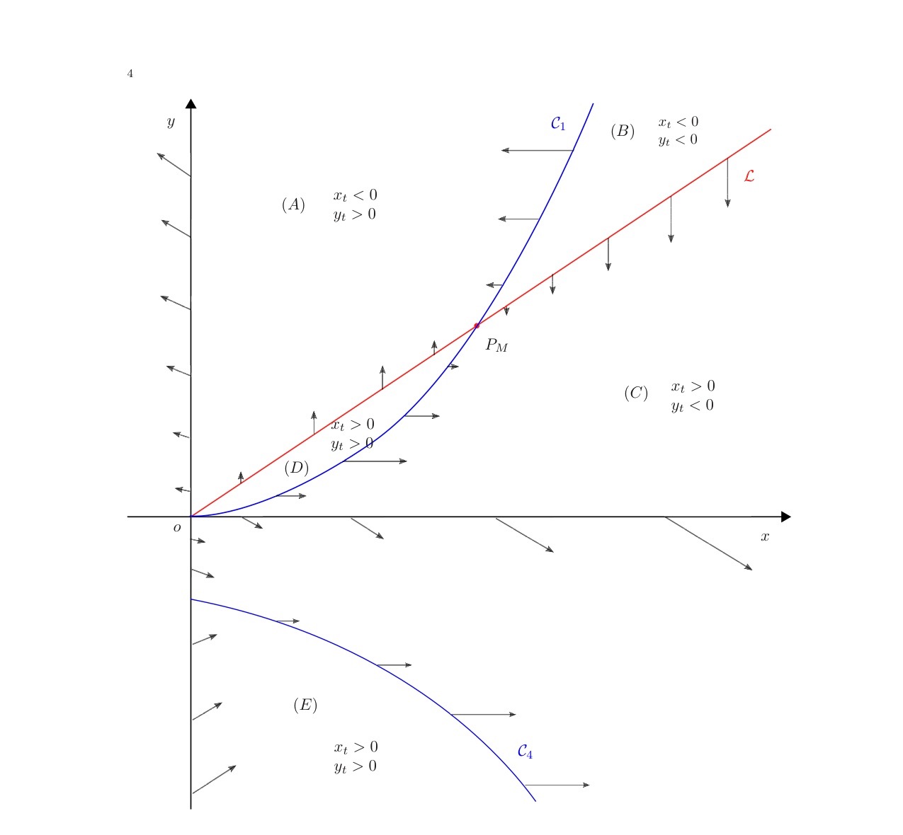
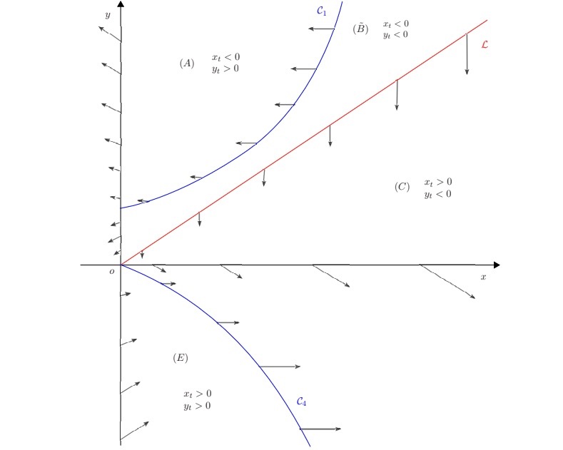
2.2.3 The vanishing curves of the vector field
The vector field associated to is defined by
| (2.22 ) |
We call vanishing curves of in the set of points where or vanishes.
and
where
and
Those vanishing curves are the boundary of some semi-invariant regions in . Their configuration depends on the intersection of these curves.
I- If and we denote by
(A) is the set of points such that .
(B) is the set of points such that and .
(C) is the union of the set of points such that and the set of points such that .
D) is the set of points such that .
(E) is the set of points such that .
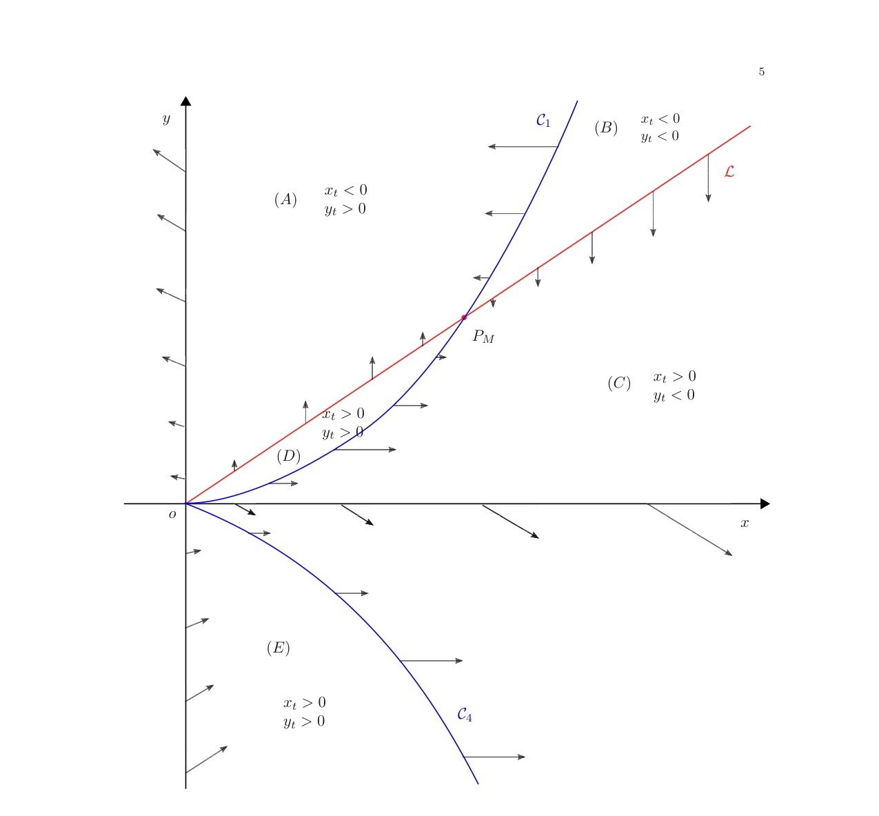
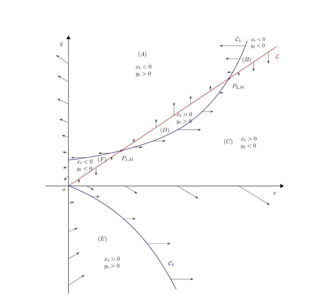
II- If and we denote by
(A) is the set of points such that .
(B) is the set of points such that and .
(C) is the union of the set of points such that and the set of points such that .
(D) is the set of points such that .
(E) is the set of points such that .
(F) is the set of points such that and .
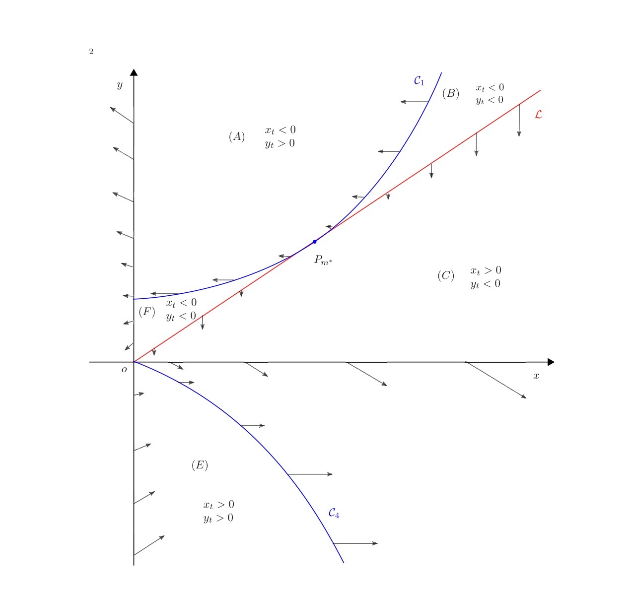
III- If and , (D) is empty.
IV- If and , (D) is empty and (B) and (F) are replaced by the set such that (note that is connected).
We present below some graphics of the vector field associated to system . We show the vanishing curves of the vector field as well as the direction of the vector field along these curves.
2.3 Description of the radial solutions defined near 0
In this section we use the dynamical system to describe all the positive solutions of defined on a maximal interval , . The case which is well-known will be used as a comparison model.
2.3.1 The case and
In this range of exponents the fixed point is unique, the problem is more rigid and some of our existence and uniqueness results hold without the assumption of radiality as shown in Theorem 4.6.
Theorem 2.4
Let and or and , and .
1- The function is the unique positive solution of in satisfying
| (2.23 ) |
2- For any there exists a unique positive solution of in satisfying . Furthermore is radial and
| (2.24 ) |
To this set of solutions is associated a unique heteroclinic orbit of the system connecting the origin when to when .
3- For any there exists a unique positive solution of in satisfying and . This solution is radial.
4- For any there exists a unique positive solution of in satisfying
| (2.25 ) |
and a unique positive solution satisfying
| (2.26 ) |
Moreover these solutions are radial.
5- Assume . For any there exists and a unique radial positive solution of in satisfying and vanishing on or such that
| (2.27 ) |
Furthermore the mapping is decreasing from onto .
Proof. 1- All the uniqueness results, which are valid not only for radial solutions, are proved in Section 4, in particular in Theorem 4.6.
2- In the phase plane , recall that is a source equilibrium and there exist infinitely many trajectories different from the regular one , converging to when , with the initial slope since , so they start from in Region (D) of Figure 1. The point is a saddle point with eigenvalues and associated eigenvectors
We denote by the trajectory such that increases and converges to when , and by the trajectory such that decreases and converges to when . Their common slope is larger than , then lies in the region and lies in the region when . Because is negatively invariant and bounded, is contained in , a region in which and are monotone. Hence converges to a fixed point in which is necessarily as . Therefore is an heteroclinic orbit joining to , and it is necessarily unique since is a saddle point. Its slope at is . It corresponds to a solution of satisfying -(i). This solution is unique by Theorem 4.6. Furthermore if then . We also notice that for any and ,
If we denote by the limit of the increasing sequence , then
This implies that is a self-similar solution of , hence and holds.
3- The trajectory converges to when and remains in the region which is negatively invariant. If were defined on whole , it would imply that it remains bounded because of the a priori estimate Proposition A.1. But in the region the two functions and are decreasing. Hence the trajectory would converge to an equilibrium in the closure of different from , which is impossible. Therefore the two functions and with image are defined on some maximal interval and if we set , the corresponding solution of satisfies . Uniqueness of a solution defined on and blowing-up at follows from Theorem 4.5. By the scaling , the function is transformed in a solution of which blows-up at and which is associated with the same trajectory . Hence can be any positive real number.
4- There exist two unstable trajectories and converging to when . They are associated to the eigenvalue , and their slope at is . We denote by the trajectory which enters in the region . Since this region is positively invariant, remains in it. Then either
its components are defined on some maximal interval and the corresponding solution of tends to when
, or they are defined on wole . In that case would coincide with by 1- which is contradictory. Hence is defined on the maximal interval . Notice also that is decreasing on some interval and increasing on by the phase plane analysis. Thanks to the scaling , can be taken arbitrarily. Since
this solution is uniquely determined by , it is unique. This corresponds to a uniqueness result for solutions of
in the class of radial solutions. This proves
Consider now the trajectory . It belongs to region when , and in this region and . Since is the only equilibrium in the quadrant the trajectory intersects the straight line
at some for some . Hence the corresponding solution vanishes for . Furthermore can be taken arbitrarily. This proves .
5- Since is a source, there exists such that any backward trajectory issued from converges to when . All these trajectories in the first quadrant have initial slope . If is above the heteroclinic orbit , it cannot converge to , then it crosses , enters in and crosses the axis for some . By Appendix A2 the associated solution of satisfies for some and . If is below , it enters the region which is positively invariant and for the same reasons as in Step 3 it blows-up for some . The corresponding solution satisfies for some and blows up for . Uniqueness of this type of solutions in follows either from the general result Theorem 4.6 or from the uniqueness of the trajectories of the system . The correspondance is decreasing and onto from to by uniqueness and using the scaling transformation .
Remark. It follows from the analysis of the phase plane that all the positive radial solutions of defined in a neighborhood of or in the complement of a ball have their behaviour described by 1 or 2.
2.3.2 The case , and
When and the isolated singularities of solutions of are removable and the behaviour at infinity of these solutions is described in [21]. When it is no longer the case and the interaction of the two reaction terms yields new phenomena. The next result covers Theorem 1.4, up to uniqueness which will follow from Theorem 4.6.
Theorem 2.5
Let , and .
1- If any isolated singularity of a solution, not necessarily radial neither nonnegative, of is removable. If is any solution of this equation in , there exists such that
| (2.28 ) |
and can only take the three values , and .
2- If , the function is the unique positive separable solution of in . There exists a positive radial solution , unique up to the scaling transformations , satisfying
| (2.29 ) |
Furthermore, for any there exists a positive and radial solution of in satisfying
| (2.30 ) |
and
| (2.31 ) |
Finally, there exists also a unique positive solution of in satisfying -(i) and or -(i) and on . In both cases the solution is radial.
Proof. The results of assertion 1 is proved in [21], [2].
Assertion 2- Since , . As a consequence, the vanishing curve goes through . Lemma 2.3 is still valid. The point is a saddle point and with and . The stable curve is an heteroclinic orbit staying in the region (D) and connecting to . The point is no longer hyperbolic since the charcteristic values are and , and the behaviour of the solutions in its neighbourhood is more delicate. The vector is the eigenvector associated to the nonzero eigenvalue and the unstable curve corresponds to the regular solutions . By the central manifold theorem, the curve is the central manifold of and is tangent at this point to the eigenvector . Therefore
on . As a consequence
Consequently in a neighborhood of . Therefore, for any there exists such that
| (2.32 ) |
Putting these inequalities become completely integrable and we derive
| (2.33 ) |
Integrating implies -(i). Uniqueness among the radial solutions follows from the uniqueness of the stable heteroclinic orbit. As in Theorem 2.4 the unstable trajectory of entering (C) intersect the axis at some and any corresponding solution is defined in some , R¿0, and it blows-up when . Using the transformation , is a solution defined in the ball which blows-up for and still satisfies . The backward trajectory of any point on the seqment converges to when . For the same reason as for the corresponding solution satisfies -(i) and it blows-up ifor for some . Since the scaling transformation leaves -(i) unchanged, can take any value, this ends the proof.
Remark.
2.3.3 The case and
In the range of exponent , the positive parameter defined by plays a fundamental role. The following result covers Theorem 1.5 and describes all the positive solutions of either defined near or near .
Theorem 2.6
Let and .
1- If , then and are the two self-similar solutions. Moreover
(i) there exists a unique, up to the transformation , positive radial solution defined in satisfying
| (2.34 ) |
(ii) For any there exists a unique positive radial defined in satisfying
| (2.35 ) |
(iii) For any there exists a positive radial solution in with j=1,2, satisfying
| (2.36 ) |
This solution is unique if . There exists also a unique radial positive solution in satisfying
| (2.37 ) |
or
| (2.38 ) |
2- If , is the unique self-similar solution, and statement 1-(ii) still holds with replaced by in . There exist infinitely many radial positive solutions in satisfying with replaced by , and at least one in satisfying or with replaced by .
3- If , there exists no singular solution. For any there exist and a unique positive radial solution in satisfying
| (2.39 ) |
Any positive radial solution defined in has the same asymptotic behaviour as in -(i).
Proof. Case 1: . (i) From Lemma 2.3-2, is a saddle point with stable trajectories , , and unstable ones and defined as in the proof of Theorem 2.4. The trajectory lies in as and remains in for all because is negatively invariant. Hence it converges to when . Therefore is an heteroclinic orbit connecting to . It is unique and it corresponds to a solution satisfying , thus is unique up to the scaling transformations for .
(ii) The point is a saddle point with unstable trajectory and stable trajectory which converges to as with initial slope . To are associated the solutions of satisfying , this solution is unique for fixed and denoted by . Since , this stable trajectory lies in the region at infinity. Since is negatively invariant, the two functions and are decreasing and thus converges to when . Hence is a heteroclinic orbit connecting to and it is unique. To this trajectory is associated a solution of satisfying and unique up to the transformations .
(iii) The unstable trajectory of enters the region (C), crosses the axis and blows-up in finite time as in Theorem 2.4. Since is a source and a node, there exist trajectories different from converging to when and with a slope at this point smaller than
. Consider one of them below near ; either it enters the region (C), then intersects the axis and finally blows-up, or it enters the region (D), but since it cannot converge to , it leaves (D) and finally blows up as in the first case. In any case such a trajectory corresponds
to a solution which satisfies with . Because of the scaling invariance of the condition, can take any positive value. Notice that since there may exist several trajectories converging to at with the same slope at this point, the corresponding solution is not unique for fixed.
As in the proof of Theorem 2.4 corresponds to a solution satisfying . The stable trajectory
of lies in the region near . Since this region is negatively invariant the trajectory remains in it, hence and are decreasing. If they were defined on , they would remain bounded by Proposition A.1 and the trajectory would converge to a fixed point in , different from . Since such a point does not exist the functions and are defined on a maximal interval and they blow-up when . To this traectory is associated a solution of satisfying with .
The trajectory is unique thus can be fixed arbitrarily by using the scaling transformation .
Case 2: . There exists a unique nontrivial equilibrium . To the eigenvalue is associated the eigenvector , while to the eigenvalue is associated the eigenvector is . There exist two trajectories and converging to
when . The trajectory with slope at enters the region (C), crosses the axis and blows-up in finite time. It corresponds to a solution with when and which blows-up at .
The point is a saddle point. The stable manifold has initial slope . It corresponds to a trajectory which converges to
when . Since the region (F) is negatively invariant this trajectory converges to when , and its slope at this point is
. Hence is the central manifold at . As in case (1) this trajectory corresponds to a positive solution in which satisfies
| (2.40 ) |
for some .
Moreover, any trajectory which has one point in the bounded negatively invariant region delimited by , and the axis , converges to when , tangentially to the line . Since it cannot converge to , it crosses the axis in finite time and it blows up for . This corresponds to a positive solution of in which satisfies with replaced by
.
We claim that there exists at least one trajectory belonging to the central manifold at which converges to
when and blows up in finite time: the backward trajectory of any , belongs locally to for since this region is negatively invariant. Furthermore its coordinates satisfy and for . Next, the backward trajectory of any belongs to and its coordinates satisfy also and for and for . Let be the set of points such that crosses for some and the set of points such that crosses for some . By standard transversality arguments and are open and disjoint.
Since is connected, it cannot be the union of the two sets and . Hence there exists in
. By monotonicity, converges to when . Clearly this trajectory cannot be defined on whole by Proposition A.1, hence it blows-up for . This proves the existence of a solution which satisfies
| (2.41 ) |
Case 3: . There exists no equilibrium besides which is a saddle point with unstable trajectory and stable trajectory with initial slope . The region between and is negatively invariant, hence remains in it and its two coordinate functions are decreasing and necessarily unbounded. The corresponding solution of cannot be defined for all because of Proposition A.1, hence it blows-up for . This proves .
Remark. It is noticeable that in the case , the equilibrium is not hyperbolic and the central manifold there consist in curves with the same slope at but one is converging to this point when while the other (may be there are many) converges when .
3 The radial case for
In this section we study the nonnegative solutions of
| (3.1 ) |
when .
3.1 Non-autonomous systems associated to the equation
Since there exists no autonomous 2-dimensional system in which equation can be transformed. The systems that we introduce below are suitable for specific range of singular phenomena characteristic of one of the following equations , and .
3.1.1 System describing the behaviour of Emden-Fowler equation
We set
| (3.2 ) |
If is a positive solution of there holds
| (3.3 ) |
where, we recall it, is defined in . Equivalently
| (3.4 ) |
where and . If this is the system which describes the radial solutions of .
3.1.2 System describing the behaviour of the Riccati equation
We set
| (3.5 ) |
If is a positive solution of , satisfies the system
| (3.6 ) |
where is defined at . The system admits a unique nontrivial equilibrium with if and only if : it is
| (3.7 ) |
The system is equivalent to
| (3.8 ) |
According to the sign of this system is a perturbation at or at of
| (3.9 ) |
which describes the radial positive solutions of .
3.1.3 System describing the behaviour of the eikonal equation
Assuming , we set
| (3.10 ) |
Then if is a positive solution of , there holds
| (3.11 ) |
where is defined at . Equivalently
| (3.12 ) |
According to the sign of this equation is a perturbation at or at of
which corresponds to the eikonal equation . We note that in the case , then , there exists an explicit radial solution of which is
| (3.13 ) |
The function is harmonic and satisfies . This solution which has already been noticed in [20] will be useful in the sequel.
Remark. The following relations between the solutions of the systems , and hold,
| (3.14 ) |
which implies
| (3.15 ) |
This yields the following relations
| (3.16 ) |
3.1.4 Lyapounov and slope functions
There are several functions the variation of which along trajectories will be analyzed in the sequel. They are specific to the change of variable we use. The most surprising one is the function described below.
Lemma 3.1
Let , , . We define on by
| (3.17 ) |
If is a positive solution of and and are defined from , set
| (3.18 ) |
Then
| (3.19 ) |
where .
Proof. There holds and
Multiplying by we get
Putting
we obtain
Since
and , we obtain
and follows.
The slope of a trajectory has shown its importance in the previous section when studying solutions of near an equilibrium. We introduce it as a Lyapounov type function the variations of which will be of particular interest for studying solutions of eikonal type.
Definition 3.2
The slope of a solution is
| (3.20 ) |
Since , there holds
| (3.21 ) |
Note that if .
3.2 Asymptotic estimates for the Riccati equation
The next lemma deals with estimates near (resp. ) of radial subsolutions (resp. radial supersolutions) of the equation , which reduces to
| (3.22 ) |
in the radial case.
Lemma 3.3
Assume , and .
1- Let be any radial decreasing function satisfying near .
(i) If , then
| (3.23 ) |
Therefore
| (3.24 ) |
| (3.25 ) |
(ii) If , then
| (3.26 ) |
Therefore
| (3.27 ) |
| (3.28 ) |
(iii) If , or if and , then admits a limit belonging to . Therefore if , admits a limit belonging to . If , has to be replaced by and if by in the previous expression.
2- Let be any radial decreasing function satisfying near . Then all the previous statements – are valid, provided is replaced by , by and, in case (iii), the limit belongs to . Furthermore if the function is bounded.
3- Let be any radial decreasing function satisfying in and tending to at infinity, and assume . Then
(iv) either and
| (3.29 ) |
for large enough,
(v) or and
| (3.30 ) |
4- Let be any radial decreasing function satisfying in and tending to at infinity. Then , and either and , or
| (3.31 ) |
for large enough.
Proof. If is a radial decreasing subsolution (resp. supersolution), there holds
Set , then
Hence the function
| (3.32 ) |
is nondecreasing (resp. nonincreasing). Notice in particular that if is a decreasing radial solution, there holds
| (3.33 ) |
and the estimate on follows by integration since .
1- If is a decreasing subsolution, is nondecreasing.
(i)- If , then
where . Since , follows.
(ii)- If , then for any , there exists such that
and follows.
(iii)- If , then as . Therefore admits a limit belonging to when . We derive the estimates on by integration.
2- If is a decreasing supersolution the results follow in the same way. If , the estimate
implies that is bounded near .
3- If is a decreasing subsolution in an exterior domain, the function defined in is nondecreasing, hence it admits a limit in .
(iv)- If
, then as , hence , therefore . If , then
. Since tends to at infinity, we obtain when .
If , then . This yields the estimate from below of , and therefore for if .
If , we obtain , and we derive a contradiction since is not integrable at infinity.
4- If is a decreasing supersolution in an exterior domain, then is nondecreasing. Hence there exists such that , which implies for some . Since the function is nonincreasing, it admits a limit belonging to . If and because , it follows that . If , then has a limit in , and this implies that admits a limit in at infinity. If , then and we obtain . If , then as , contradiction.
3.3 Estimates near
3.3.1 The case
Here we prove Theorem 1.7. If is a positive solution of unbounded near , then , hence the variable and defined in satisfy
| (3.34 ) |
where, we recall it, and . Since , remains bounded when . The difficulty comes from the fact that the term tends to infinity when .
Lemma 3.4
Assume . If is a positive solution of in such that , then admits a limit when which can take only the values or .
Proof. We use the function introduced in . Because of Proposition A.1 and Proposition A.3, and are bounded. By assumption is nonnegative, hence is bounded when . Using we have that
which implies that
| (3.35 ) |
for some . Because , we deduce that the function is decreasing, therefore it admits a finite limit when , and is also the limit of . Hence
| (3.36 ) |
Therefore converges to some satisfying . The omega-limit set at of the trajectory is the set of couples such that there exists a sequence decreasing to such that . It is non-empty since the trajectory is bounded, connected and compact. By La Salle’s theorem, the function which is monotone decreasing is constant on . This implies , hence . Because then , hence and when . If , it implies that
Hence where . Clearly this implies that cannot be bounded, contradiction. Therefore . This implies that
| (3.37 ) |
which ends the proof.
Lemma 3.5
Assume , and let be a positive solution of in unbounded near .
1- If and near , then necessarily and
| (3.38 ) |
Therefore
| (3.39 ) |
| (3.40 ) |
2- If and is bounded for any , then
| (3.41 ) |
| (3.42 ) |
3- If and is bounded if or is bounded for any if , then there exists such that
| (3.43 ) |
and
| (3.44 ) |
Proof. We first notice that if is unbounded near , then in a neighborhood of and we can apply the results of Lemma 3.3 concerning subsolutions. Moreover, if when , then for any there exists such that
| (3.45 ) |
and we can also use the results of Lemma 3.3 dealing with supersolutions.
1- Since is a decreasing subsolution of , near , hence . By assumption . Then near , hence applies. It follows by Lemma 3.3-(1)-(2) that
| (3.46 ) |
Since is arbitrary, this implies . The other estimates and are obtained by integration.
2- By , . From the assumptions, for any , , then
Next implies that . Therefore, we can take small enough such that . This implies that holds in . Hence we get and by integration.
3- Suppose then if . By Lemma 3.3-(1), near , hence
Since , we deduce that for any , holds in . Then we use Lemma 3.3 and obtain and by integration. In the case there holds
for any . Choosing , we find again .
For obtaining the next result, the key is the introduction of the slope function which allows to make precise the behaviour of solutions such that .
Lemma 3.6
Assume , and . If is a positive solution of unbounded near and such that when , then and the following trichotomy holds.
1- If , then or is satisfied.
2- If , then or is satisfied.
3- If , then or is satisfied.
Proof. By assumption as . We recall that satisfies hence
| (3.47 ) |
1- We first assume that as . Then for any , there exists such that on . Hence is increasing. This implies that is bounded near and thus by Lemma 3.5. If it would follow from Lemma 3.5 that holds, which is not possible. Hence , and holds. If and , cannot hold; hence and holds. If , cannot be satisfied, hence and holds.
2- Now we assume that . Then there exist and such that for . Hence therefore as . This implies as . Then holds. Using Lemma 3.3-(1)-(2), we have or if , or if and or if .
3- Next we assume that . Then there exists a decreasing sequence converging to such that and , which is a local maximum of , tends to . Put and , then
| (3.48 ) |
with . This implies in particular and . Since it holds for all local maximum of we deduce , which implies . If (resp. ) we obtain from Lemma 3.5-(3) (resp. from Lemma 3.5-(2)). If we write under the form
| (3.49 ) |
From , for large enough and when , hence
| (3.50 ) |
This implies that for any there exists such that for . Hence as . Since , it implies that as . Therefore and hold.
3.3.2 The case
Proof of Theorem 1.8. If and it is proved in [7] that positive solutions of in can be extended as a solution in . Next we suppose that , or , hence . We use the change of variable and satisfies . It is important to notice that is negative, therefore the system satisfied by is a perturbation at of the system
| (3.51 ) |
where , associated to the Emden-Fowler equation by the same change of variable. Since is bounded, the omega-limit set at of the trajectory is a non-empty compact connected subset of the set of stationary solutions of . Therefore
| (3.52 ) |
If the result is proved, thus let us assume that . By Lemma 3.3-1-(iii) admits a limit when . If , follows by integration. Thus we are left with the case . Hence if , or if . Therefore, for any , is bounded from below in by the function which satisfies in , on and if , or if . Letting , , and by [22]. This is a contradiction.
3.4 Estimates at infinity
3.4.1 The case
Proof of Theorem 1.9. We recall that by Proposition A.1 and Proposition A.3 in the Appendix all the positive solutions of in satisfy
| (3.53 ) |
where , and by the maximum principle they are decreasing. Since is continuous in , is well defined and positive. By the maximum principle, for any , is bounded from below in by the solution of
| (3.54 ) |
When , which satisfies in and on . Then and by [21], satisfies
| (3.55 ) |
We make the change of variable and obtain the system satisfied by the functions . Since , is positive. Hence the omega-limit set of the trajectory of as is a non-empty compact connected set of the set of solutions of stationary solutions of , therefore
| (3.56 ) |
Therefore if we obtain , and if we have that .
If , then . From Lemma 3.3-(3), we have that either and holds, or and holds. However, since , one has when , hence does not hold and we deduce that is verified.
Finally we consider the case . Then and satisfies
| (3.57 ) |
and . Since is bounded from below by , we have that , with , for large enough. Hence for any there exists such that
| (3.58 ) |
Therefore where
| (3.59 ) |
The asymptotic expansion of is obtained in [21, Lemme 3.2 ] using an old result due to Hardy. We give below a simpler proof.
| (3.60 ) |
This implies that for any there holds
| (3.61 ) |
which implies .
Remark. The proof of Hardy’s theorem quoted in [3] is not easy to find. An alternative proof is to consider the following equation, to which reduces by a suitable scaling transformation,
| (3.62 ) |
where and . Since as , it is easy to see that for any , by considering supersolutions under the form
Since is a subsolution for some , it is smaller than . Furthermore, for any , there exists such that is a supersolution on and is larger than . From that we infer
| (3.63 ) |
An alternative proof of the convergence is to set . We get
where . Applying [10, Corollary 4.2] we deduce that converges to a limit which satisfies . From the lower bound and we infer that is impossible.
3.4.2 The case
Proof of Theorem 1.10. If , then . Therefore . Hence if a nonnegative solution of on , is bounded for . Therefore the natural system for describing the solution is the system with bounded and and we use an argument similar to the poof of Lemma 3.4.
Lemma 3.7
Assume , and . If is a positive radial solution of in , there holds
| (3.64 ) |
Proof. By Proposition A.3 is bounded, hence still holds on . We consider now the function defined in , then is decreasing and bounded at infinity since . Therefore converges to some real number when . This implies that identity is still valid provided is replaced by . Mutatis mutandis, the remaining of the proof of Lemma 3.4 still holds and we get .
Lemma 3.8
Let the structural assumptions of Lemma 3.7 be satisfied. If is a positive radial solution of in , such that
when , then necessarily and the following alternative holds:
1- either and
| (3.65 ) |
where we recall that is defined in ,
2- or and
| (3.66 ) |
Proof. Since , we can apply Lemma 3.3-(3) provided . If this holds the following estimate from below of holds:
either and ,
or and .
1- We first prove that is bounded and we recall that denotes the slope function.
1-(i) If as , then for any , is nondecreasing. Hence for , for some
. This contradicts Proposition A.1
1-(ii) If . Then there exists and such that on . Hence
for and as . Using Lemma 3.3-(3)-(4) we infer that and or holds, and in both cases is bounded.
1-(iii) If satisfies . There exists an increasing sequence tending
to infinity of local maximum of . As in the proof of Lemma 3.6-(3) we obtain that and .
If , equivalently , then for .
If , we have from and that
. Hence is increasing with limit . Since at the points of local maximum of
, we also have , we obtain the implication
| (3.67 ) |
Hence is finite, which implies again that is bounded.
2- Convergence. Since is bounded, the trajectory endows this property, and since , its omega-limit set at infinity is non-empty, compact, connected and it is a subset of the nonnegative stationary solutions of .
If the set is reduced to . Since , we deduce from that is monotone decreasing. It follows from that , hence as in 1-(ii) and by Lemma 3.3-(3)-(4) necessarily , contradiction.
If , then either converges to or it converges to , in which case by Lemma 3.3. The function is bounded from below in by the solution of
Since and , this ends the proof.
3.5 Solutions of eikonal type
In order to study the properties of solutions of eikonal type we first give some asymptotic expansion results.
Lemma 3.9
Let , (resp. ) and (see for the definition of ). If is a solution of which converges to when (resp. ), then has a constant sign for large enough. Furthermore
| (3.68 ) |
Equivalently, with ,
| (3.69 ) |
Proof. (i) Expansion of . Set
Then
If is not monotone, one has at the local extremum of , denoting , and ,
But , then when . Therefore . Since the limit is valid for local minima or maxima it follows that .
If is monotone, then admits a limit when . Since , it follows that has a also a limit at and the only possible one is . Hence . In both case it yields, since ,
| (3.70 ) |
(ii) We claim that has a constant sign. If is nondecreasing (resp. nonincreasing) then (resp. ) for . Actually the inequality is strict, otherwise, if there is some such that , we would have for and for . If this contradicts the fact that . If we deduce from that if is a local minimum we have
This implies that . Similarly, if we get .
(iii) Asymptotic expansion. We write and . Then
| (3.71 ) |
There holds
where and , therefore and for . Next, from ,
where , and and when . Therefore the previous identity becomes
| (3.72 ) |
where when . Next
where and . It follows from that
| (3.73 ) |
This leads to the following two inequalities verified by
and
and we know from (i) that keeps a constant sign when . We deduce from the above inequalities that if the function is decreasing for some and tends to , hence it is negative, while, if , is increasing for another and tends to , hence it is positive. Then, we can summarize as follows, with a new
| (3.74 ) |
As we have , the function is increasing and tend to as . Hence it is positive. In the same way, the function is decreasing, tends to hence it is negative. Therefore we infer that
| (3.75 ) |
This implies . From , , then and . Since , we deduce . Notice also that from there holds
hence
| (3.76 ) |
In particular has the sign of , and therefore is monotone.
3.6 Local or global existence results
3.6.1 The systems of order 3
Since , we can perform the transformation and assume that . For proving the existence of solutions to there are essentially three methods: the methods of sub and super solutions which has already been developed in Section 2.3, the method of fixed points, and the use of a specific autonomous system of order 3. This last method appears to be entirely new and we explain it below. This system uses the variables ,
| (3.78 ) |
Lemma 3.10
Let with and . If is a decreasing positive solution of , then
| (3.79 ) |
satisfies . Conversely, to each trajectory of in corresponds a unique solution of .
Proof. Let be a decreasing solution of . We recall that are solutions of , and with . Then satisfies the following system which is equivalent to ,
| (3.80 ) |
Using we have that . Since by computation , we deduce that satisfies .
Conversely, let be a solution of , then
Hence for some . If we set , we see that
Hence
| (3.81 ) |
Setting , , then
| (3.82 ) |
Then the function satisfies . Let and be two solutions of . Then there exist such that
and
If and correspond to the same trajectory, there exists such that for all , thus
Therefore . Hence
In conclusion, there is a one to one correspondence between the trajectories of and the solutions of .
Remark. Using the relation one can see that is equivalent to the following system in the variables ,
| (3.83 ) |
This system is particularly suitable for constructing local solutions in or , in particular when , in the case .
3.6.2 Singular solutions of eikonal type
Proof of Theorem 1.11. We recall that these solutions of eikonal type are the solutions which behave like near or . For and we set and . Then there exist depending on such that
(i) Subsolutions. If , then
| (3.84 ) |
Set . Then and achieves its minimum at with minimal value . Notice that if i.e. , then
we find the explicit solution defined in .
(i-a) If or , or if and , then and is a subsolution in provided .
(i-b) If and there exists such that is a subsolution in Hence
is a subsolution in .
(ii) Supersolutions. We have
| (3.85 ) |
(ii-a) If , then for and any , is a supersolution in .
(ii-b) If and , then for any we take such that , hence in . Since , we take such that , hence in . Consequently is a supersolution in .
(ii-c) If and , then we can take such that and obtain that is a supersolution in .
(iii) Proof of statements 1 and 2.
If and whatever is the sign of there exist and such that is a supersolution in larger than the subsolution . By [25, Theorem 1.4.5] there exists a radial solution in satisfying . Its behaviour at infinity is given by Theorem 1.9. This solution is decreasing by the maximum principle and it is unique by Theorem 4.6-(3).
The existence of a solution in a bounded domain containing and vanishing on satisfying follows by Theorem 1.14 which is proved in Section 4. So we deduce statement 1.
If and , one has a supersolution in and a subsolution in .
Up to increasing the value of one has again a supersolution larger than the subsolution . Hence there exists a solution in between satisfying which proves statement 2.
3.6.3 Riccati type singular solutions
Proof of Theorem 1.12. We recall that the Riccati equation admits the radial solution if and only if . This function is a supersolution of in .
1- Local existence in a neighborhood of . Since the system in variables admits the equilibria , and . Our aim is to construct local radial solutions of satisfying and , equivalently
| (3.86 ) |
Conversely, any solution satisfying corresponds to a solution satisfying . The system may be singular at or at ; hence we desingularize it by setting and . Then satisfies
| (3.87 ) |
So we are led to study solutions in a neighborhood of the equilibrium where . We set , and in order to reduce the study at , and satisfies the following linearized system
| (3.88 ) |
If we denote by the matrix of this system, then its charecteristic values are the roots of the polynomial
| (3.89 ) |
with , and . Since all the eigenvalues are positive. We find that
are eigenvectors corresponding to and respectively. If and , we can take for eigenvector corresponding to the vector for some real numbers and . Actually
Then there exists one trajectory of with when such that when . Hence there exists at least one solution of such that when .
2- Local existence at infinity. Here we assume . Then , and . Then there exists a unique local trajectory which converges to when , it corresponds to the stable manifold of this point. If there exists a positive solution in , the solution can be extended as a solution in by [7, Theorem 1.1] since in this range of values of one has . By Proposition A.1 such a solution is identically .
Remark. Note that we have many types of trajectoriess converging to the origin and their geometry depends in their sign and their relative order. In this respect we denote
| (3.90 ) |
and we have
| (3.91 ) |
We have that only if and , a condition which is compatible with only if .
Global (necessarily singular) solutions in are difficult to construct. We give below a range of exponents in which there exists at least one.
Theorem 3.11
Let , and , . If there holds
| (3.92 ) |
in particular if and , then there exists a positive radial solution of defined in satisfying
| (3.93 ) |
Proof. The function is a supersolution of in . We look for a subsolution under the form for some . Set
where
Then on the interval one has
In order , one needs
Since , if we set , then on and the previous inequality to be verified becomes
We first impose , then on . We set
| (3.94 ) |
Then
and
Since , is convex on . Furthermore . Hence if .
| (3.95 ) |
Replacing by its value, will be achieved, provided is large enough, if
| (3.96 ) |
The condition is that with satisfying . It necessitates , equivalently
, and
(i) either , then we can choose any ,
(ii) or , then we can choose any .
These conditions are satisfied if which is equivalent to .
If one of the above conditions is satisfied, it follows by [25, Corollary 1.4.5]
that there exists a radial positive solution of in which satisfies
| (3.97 ) |
Remark. Condition is equivalent to
| (3.98 ) |
Condition (ii) is equivalent to
| (3.99 ) |
Note that the nature of the variations of the function differs according to the value of .
If or , is increasing and onto from to when and from to when .
If , achieves a maximal value for with
| (3.100 ) |
In particular one has
3.6.4 Emden-Fowler type singular solutions
Proof of Theorem 1.13-(1). Since the function is a subsolution of in . In order to be a supersolution, one needs
| (3.101 ) |
The function is increasing and onto from to . Hence there exists such that . For such a value we have that
Since the function is a supersolution of in . For we set . Then
| (3.102 ) |
Clearly in , and for , one has
Therefore, if , the function is a supersolution in . Since , it follows by [25, Theorem 1.4.5] that there exists a solution of in such that . Then by Theorem 1.8-(1), u satisfies -(i), and by Theorem 1.10-(2), -(ii) holds. Furthermore for any . Uniqueness (not only for radial solutions) is a consequence of Theorem 4.6-(2). Obviously is decreasing. Existence of a positive solution in a bounded domain containing is a consequence of Theorem 1.14, see Section 4.
3.6.5 Solutions behaving like the Newtonian potential
There exist also solutions which behave like the Newtonian kernel at . They are described in the next result.
Theorem 3.12
Let and . Then for any and there exists a minimal positive solution of in such that holds. Furthermore it is radial and nonincreasing. If we assume , this solution is unique among all the positive solutions.
Proof. Proof of existence. If the result is classical and for we denote by the solution of in satisfying . This is a natural subsolution of .
The construction of the supersolution is more involved.
(i) We first assume that and prove that for any there exists such that for any there exists a supersolution of satisfying . Let set
Then there exist depending on and such that.
| (3.103 ) |
Note that we have only used inequalities .
Set . Then, for we take and we derive that .
The supersolution satisfies .
(ii) If and for we denote by the solution of
| (3.104 ) |
and we set . Since , and as . Hence
| (3.105 ) |
Furthermore, by Keller-Osserman technique combined with scaling method, there holds in ,
| (3.106 ) |
In the above inequalities, and are positive constants depending on and . Hence
| (3.107 ) |
We infer
| (3.108 ) |
and
| (3.109 ) |
If is fixed, and we conclude that is a supersolution in larger than .
We deduce from (i) and (ii) that for any there exists such that for any there exists a positive radial solution of satisfying . Furthermore satisfies . Therefore is necessarily decreasing.
End of the proof of existence. Let and such that . For let such that for any there exists a positive radial solution to satisfying . If there holds
where . Then
which implies that is s supersolution of and . We conclude as in the first step.
Uniqueness. It is proved in Theorem 4.6, this ends the proof.
When we do not assume we have only the existence of a minimal positive solution. This is due to the fact that for two solutions
and as above, is a supersolution larger that . The conclusion follows easily.
In the next statements we prove the existenc of radial solutions defined in the complement of a ball of , which behaves like the Newtonian potential at infinity. We start with the following lemma dealing with the positive radial solutions of in the complement of a ball.
Lemma 3.13
Assume and . Then for any there exists such that the unique solution of in verifying satisfies
| (3.110 ) |
Furthermore the mapping is continuous and increasing from onto for some .
Proof. The existence and uniqueness of a solution in an exterior domain and the fact that holds is classical (see e.g. [21]). However the fact that and the continuity of is not proved there. By the maximum principle is nondecreasing. Next we set and . Then satisfies
| (3.111 ) |
where . By the maximum principle ( is the positive harmonic function in with value on ), hence is bounded. Since is convex and bounded, it is decreasing and as . Hence
| (3.112 ) |
Hence by integration the function is increasing and bounded. Then it has a finite limit when and has the same limit . Thus and consequently . Let be a decreasing sequence in converging to . Then the sequence of corresponding solutions is decreasing to the sequence is nonincreasing with limit . From one get
| (3.113 ) |
and the same identity holds in is replaced by . By the dominated convergence theorem, one has that
| (3.114 ) |
which implies that . A similar result holds if is an increasing sequence in converging to . Hence is increasing and continuous. When increases and converges to the unique positive solution of in such that . Hence and .
Remark. Since the equation is invariant by the transformation defined in , the ball can be replaced by for any . The range of , that we call is modified accordingly and . Then one has
| (3.115 ) |
Theorem 3.14
Let , , and .
1- For any there exist and a positive radial solution of in satisfying
| (3.116 ) |
2- If there exist and a positive radial solution, unique among all the positive solutions, of in satisfying and with . In the particular case we have (see ).
3- If and the assumption of Theorem 3.11 is satisfied, there exist and a radial positive solution of in satisfying and . Furthermore is unique among all the positive solutions satisfying .
Proof. 1- If is a positive radial and decreasing function such that it satisfies (see )
where, and . If , is defined on . Hence if as , one has
| (3.117 ) |
Then as . Hence, if is given, we choose such that
. In order that is in the range of the application , one takes such that
. For such an , there exists such that the solution of in verifying
on satisfies . We then set . The function defined by is a supersolution of in , larger than the subsolution and both and satisfy . Then by [25, Theorem 1.4.5] there exists a radial positive solution of in such that , hence follows.
2- The existence of a unique positive and radial solution in satisfying follows from Theorem 1.11. The asymptotic behaviour is a consequence of Theorem 1.9-(2).
3- Under the condition of Theorem 3.11 there exists a unique positive solution in satisfying . From Theorem 1.9, and since , its behaviour at infinity is given by for some specific . Uniqueness follows from .
4 Isolated singularities of non-radial solutions
4.1 Existence and uniqueness of singular solutions
The results of this paragraph are independent of the description of the radial singular solutions performed in the previous sections and they provide a general tool for constructing singular solutions. The existence of singular solutions is based upon the next variant of [11, Theorem 2.1] proved in [25, Corollary 1.4.5].
Theorem 4.1
Let be a bounded domain in , a real valued function, an increasing function such that
| (4.1 ) |
Let be the operator defined by
| (4.2 ) |
If there exist a supersolution and a subsolution such that , then for any satisfying there exists a function verifying , solution of and such that .
One of the main application of this result is Theorem 1.14 which is proved below
Proof of Theorem 1.14. Let be a sequence decreasing to and such that and set . Then on and the function satisfies in . The function satisfies . Put . Then , and on . By Theorem 4.1 for any there exists a function such that satisfying in . Furthermore is unique by the maximum principle. Since on , , and therefore , is radially decreasing and on we infer that in if . Hence the sequence is increasing and it satisfies
| (4.3 ) |
By standard regularity estimates, is relatively compact in . Hence it converges to a solution of in which coincides with on and satisfies .
As a first application we have the following:
Corollary 4.2
Let be any bounded smooth domain containing and be nonnegative. There exists a positive solution of in with value on such that remains bounded in where is equal to or (j=1,2) or according to we are in the cases (1)-(2) or (3) or (4) of Theorem 1.1.
The existence of singular solutions is not restricted to the case where they are explicit. The following easy to prove corollary shows that existence, and sometimes uniqueness, holds when . This range of exponents is analysed in [7] in connection with problems with Dirac measure data.
Corollary 4.3
Let , , be any bounded smooth domain containing . Assume if or any if , if or any if , and . Then for any , , there exists a positive solution of in with value on satisfying .
More general uniqueness results valid for any positive solution, not necessarily radial, are obtained below. Furthermore the problems involved are either considered in or in a punctured bounded domain. If is a positive parameter we define a continuous group of transformations acting on functions defined in an open set , , for by the formula
| (4.4 ) |
If satisfies in , then satisfies
| (4.5 ) |
If , is a supersolution of if and only if
| (4.6 ) |
This conditions are compatible if and only if . Similarly, if , is a supersolution of if and only if
| (4.7 ) |
This conditions are compatible if and only if .
Proof of Theorem 1.15 First we note that two terms on the right hand-side of in the statement of the theorem coincide only if since is equivalent to . We first study the problem in
. We have to consider two cases:
1- Suppose . We choose such that
| (4.8 ) |
Let and be two positive solutions satisfying . For , is a supersolution. Since
and as , for any the function which is a supersolution is larger than near and at infinity. Then in . Letting and , yields . Similarly
.
2- Suppose . We choose such that
| (4.9 ) |
Then for , is a supersolution in which is larger than at and at . Hence
and we conclude as in the first case.
Next we consider the problem in . Since the solutions are continuous in , for we have that for
near provided is small enough. Hence in .
This implies that by letting and then . If then , and we compare
and in . The proof follows.
The previous result necessitates to find some satisfying either or which is not always possible in practice. We give below a variant of the result which necessitates a slightly sharper blow-up estimate.
Theorem 4.4
Assume , , and . Let such that
| (4.10 ) |
There exists at most one positive solution of in satisfying
| (4.11 ) |
or
| (4.12 ) |
where are some positive constants and and .
Proof. The principle of the proof is to replace by
| (4.13 ) |
when . Then, for , is a supersolution. If satisfies then, as ,
Since , is larger than another solution near . Thus for any , which implies the claim.
If satisfies , then
Again is larger than another solution in a neighborhood of and we end the proof as in the first case.
Remark. The method developed above allows to give uniqueness result for large solutions under some starshapedness assumption. Let be a domain with compact boundary and , we consider the problem
| (4.14 ) |
Such a solution, if it exists is called a large solution.
Theorem 4.5
Assume , and and is a bounded domain starshaped with respect to . There exists at most one positive function satisfying in one of the following case:
1- and .
2- and .
Proof. Let and be two positive solutions of . In the first case with . Then for and , is a supersolution of in . Since
, , it follows that .
In the second case with , then for and . Then is a supersolution in . Then for , in . Letting and yields .
This ends the proof.
If we combine the results of existence of radial singular solutions in with the uniqueness results of Theorem 1.15 and Theorem 4.4 we have the following:
Theorem 4.6
Assume , and . There exists one and only one positive solution of in , if one of the following conditions holds:
1- , , and satisfies -(i) for some .
2- and .
3- , , and either , or satisfies -(i) for some .
4- , , and satisfies -(i).
Furthermore, existence and uniqueness of a solution holds if the equation is considered in where is a bounded smooth domain starshaped with respect to and is the function is equal to some on where is nonnegative.
Proof. By applying Theorem 1.14 and Theorem 1.15 the proof is reduced to use results of existence of radial positive singular solutions in and to check that the parameters fulfill the conditions of Theorem 1.15.
Case 1- If , and . Existence of radial positive solutions satisfying -(i) is proved in Theorem 1.3.
Case 2- Then . Existence of a radial positive solution satisfying is proved in Theorem 1.11-1.
Case 3- If , then , and since , . Existence of a a radial positive solution satisfying is proved in Theorem 1.13-1. Furthermore the assumptions on and imply that . The existence of a positive solution satisfying -(i) for any is proved in Theorem 3.12.
Case 4- When , there exists a radial global solution satisfying -(i) by Theorem 1.4. We apply estimate in Theorem 4.4 with and . The result follows.
Remark. In the case , we conjecture that the function is the only positive solution of defined in satisfying .
4.2 Characterization of singular solutions
In this section we give some results showing how the characterization of singularities of radial solutions can be extended to nonradial solutions. An important tool for studying positive isolated singularities is Harnack inequality.
Proposition 4.7
Assume , and . If is a positive solution of in , there exists such that for any there holds
| (4.15 ) |
4.3 The case and
In this section, the results are obtained by a combination of Theorem 3.12 for existence of solutions and Theorem 4.6 for their uniqueness.
Theorem 4.8
Let , , , and be a bounded domain containing . For any there exists a unique positive function solution of in , vanishing on and satisfying
| (4.17 ) |
Furthermore is increasing by the maximum principle and converges to a solution of in , vanishing on and satisfying
| (4.18 ) |
where is defined at , or
| (4.19 ) |
where , are the unique positive root of equation with and respectively.
Proof. Let be such that . By Theorem 1.13-1 and Theorem 4.6, for there exists a unique solution (resp. ) of in (resp. ) satisfying -(i) and vanishing on (resp. ). If we extend by in , we have,
All the above functions are locally bounded in and by Proposition A.1. Since the mappings and are increasing, we have, by letting ,
Then we obtain by Theorem 1.7-(1) and by Theorem 1.8-(1) and Theorem 1.3.
The main characterization of isolated singularities is the next result.
Theorem 4.9
Let , be an open subset containing , , and . If is a positive solution of in , then either its behaviour at is given by or , or there exists such that holds. If the singularity at is removable.
The proof needs a few intermediate steps.
Lemma 4.10
Let , be an open subset containing , , and . If is a positive solution of in vanishing on and such that
Then there exists such that holds. If , then coincides in with a solution of in .
Proof. By assumption and by [4, Lemma 3.10] we have the following: if is a solution of in (not necessarily positive) such that is bounded near for some , then is also bounded near . Actually, in the reference the result is proved for a more general operator, without the absorption , but the adaptation is straightforward. The result applies there with and in particular . We write under the form . Since and we have
for some . It follows by Serrin’s result that either the singularity at is removable, or there exist such that
In order to make the convergence precise, we denote by the solution of
Then where
and
Because and , and satisfy
for some and , . Then satisfies
The function is harmonic in and is bounded from below by which satisfies . Hence by standard result on singularities of harmonic functions, admits a limit
when . Combined with Serrin’s estimates it follows that either and the singularity is removable,
or . Note that if , then is a solution in .
Another proof based on a perturbation is the following: let with and . Then
Since , we can write
where and is bounded. Then the result follows by [10, Proposition 4.1].
We give below another application of the perturbation method and specific to the case .
Proposition 4.11
Assume is an open subset containig , , and . If is a solution of
| (4.20 ) |
not necessarily nonnegative in , then converges uniformly with respect to when to a non-empty compact and connected subset of the set of solutions of
| (4.21 ) |
If , is either or .
Proof. We can assume that and set with . Then satisfies
| (4.22 ) |
in where and . By assumption , hence is an exponentially small perturbation of the autonomous equation associated to the Emden-Fowler equation by the same change of variables. The result follows from [10, Theorem 4.1] but for the sake of comprehension, we recall its proof. By Proposition A.2 the function is uniformly bounded, and by and are also uniformly bounded. By standard local regularity theory for elliptic equations, there holds
where is the covariant derivative of order on . Then the omega-limit at of the trajectory in is a non-empty compact connected denoted by . From we have that
where
Because and is uniformly bounded, there holds
Multiplying by and using the previous estimate, we obtain
As and are uniformly continuous in , this implies that
Therefore . If , then for any and the result follows by the maximum principle.
Lemma 4.12
Let , , be a bounded open subset containing , , and . If is a nonnegative solution of in such that
| (4.23 ) |
then
| (4.24 ) |
Proof. Without loss of generality we can assume that . It follows from Proposition 4.7 that Hence there exists a decreasing sequence converging to such that
Let be the solution of
| (4.25 ) |
where is the explicit constant such that , where is the Newtonian potential in ; note that is radial because of uniqueness. Then the sequence is increasing and converges to the function which satisfies (see [22])
| (4.26 ) |
Moreover, and since is a subsolution of , we have that in . Letting implies that in . Therefore
Combined with Proposition 4.11, this inequality implies .
This result admits an extension to the case .
Lemma 4.13
Let , , be a bounded open subset containing , , and . If is a nonnegative solution of in such that
| (4.27 ) |
then
| (4.28 ) |
Proof. Assuming for simplicity that and using Proposition 4.7 we obtain that for some decreasing sequence converging to we have
Therefore, is bounded from below in by the (radial) solution of
| (4.29 ) |
The sequence may not be monotone, but where has been defined in . Since is eventually locally bounded in by Proposition A.1 and standard regularity results (see e.g. [13]), up to a subsquence, it converges locally uniformly in to a radial function which satisfies
| (4.30 ) |
and
| (4.31 ) |
By Theorem 2.4-(4) we have that
| (4.32 ) |
The upper estimate is obtained as follows. By Proposition 4.7 the function is bounded from above in by where is the solution of
| (4.33 ) |
For the same reason as above there exists a subsequence, which converges locally uniformly in to a radial solution of . By Theorem 2.4-(4) we have that . Then which ends the proof.
When and is not bounded, Harnack inequality may not hold. However we still have a dichotomy for the possible behaviour which extends Theorem 4.9.
Theorem 4.14
Let () be an open set containing , , and . If is a nonnegative solution of in , then the following dichotomy holds:
1- either there exists such that converges to in measure on as ,
2- or .
Proof. We recall Richard-Véron’s isotropy theorem [20, Theorem 1.1]:
Let be a continuous nondecreasing function satisfying
| (4.34 ) |
If is a nonnegative function satisfying
| (4.35 ) |
where is a nonnegative radial function, then we have the following:
(i) either converges in measure on to some as ,
(ii) or
| (4.36 ) |
Since , assumption is satisfied with and equation with . Then either the statement 1 holds, or holds. If it is the case, then for any , is bounded from below in by the solution of in vanishing on and satisfying . Such a solution exists and is unique by Theorem 4.8. Letting , this implies
| (4.37 ) |
Next, we denote by the solution of on (hence is 1-dimensional) satisfying
Its existence is proved in Theorem 1.10, Theorem 1.11. It is decreasing. For the function satisfies in and when . If for some such that , then is a supersolution of in which is larger than for and . Hence in . Letting yields for and finally
| (4.38 ) |
Combining and we obtain .
Remark. We conjecture that the convergence in Theorem 4.14-1 holds in the strong sense.
Remark. Most of the results of this section can be extended to the case . The subcritical case corresponds then to and . The main change is that has to be replaced by .
4.4 The case and
The cases that we consider are , and . We recall that the stationary equation admits two positive constant solutions if and , and only one denoted by if and or if and . The following result is an improvement of Proposition A.1
Lemma 4.15
Let , , be a bounded domain containing such that and .
1- If and , then any positive solution of in satisfies
| (4.39 ) |
2- If and , or and , the same inequality holds with replaced by and respectively.
Proof. We assume first that .
1- Construction of the maximal solution. We claim that is the maximal solution of in . For
we set . Then
Taking large enough we obtain that is a supersolution in . We set for and as in the proof of Theorem 4.14 we deduce that the function defined by
is a positive and radial supersolution of in which tends to infinity on . It dominates any positive solution of in . Next we set
It is a subsolution of in dominated by . Since the supremum is achieved for , the function is radial and positive. By [25, Theorem 1.4.5] there exists a solution of in such that
The function is positive and radial. Since any positive solution in is dominated by , the function is larger than in . This implies the relation, valid for any ,
| (4.40 ) |
When the sequence decreases and converges to a positive radial solution of in which dominates any other positive solution. Hence is the maximal solution in . Letting in we infer that for any . Hence is self-similar. Since it is radial and larger than any other positive solution, we deduce that
| (4.41 ) |
2- End of the proof. If is any positive solution in , then is a supersolution larger than in . Letting yields the result. The proof in the other case is similar.
Theorem 4.16
Let , , be a bounded domain containing , and . If is a positive solution of in , there holds
1- If
| (4.42 ) |
then can be extended as a solution of in .
2- If
| (4.43 ) |
then
| (4.44 ) |
3- If
| (4.45 ) |
then there exists a sequence converging to such that
| (4.46 ) |
4- Any one of the two following situations never occur
| (4.47 ) |
Proof. 1- If relation holds, it follows by Harnack inequality proved in Proposition 4.7, that there exists a sequence converging to as such that
| (4.48 ) |
For any and , the function
is a supersolution of in which is larger than near and on . Hence
. Letting implies , and the result follows by standard regularity.
2- If holds there exists a sequence converging to such that
Furthermore, we can assume that when . Using Lemma 4.15 there exist a nondecreasing sequence converging to and a bounded sequence such that . We set with , then there holds,
| (4.49 ) |
on . By standard regularity estimates and Ascoli-Arzela theorem there exist a subsequence of and a nonnegative function such that converges to in the topology of , for any , and is a solution of in . Furthermore . By Lemma 4.15, is the maximal solution of in , it then follows from the strong maximum principle that and uniformly in . Let , then there exists such that for any , we have that for any . Since is a subsolution of , it follows that for , one has
Letting yields
| (4.50 ) |
Since is arbitrary we infer that
| (4.51 ) |
By assumption ; then holds.
3- Let us assume that the first condition in holds. If the function
| (4.52 ) |
is asymptotically monotone, nonincreasing or nondecreasing, then either in the first case, or in the second case. Using again the uniform estimate and Ascoli-Arzela theorem we have that there exists a sequence converging to such that converges in the -topology of , for any , to a positive solution of in such that and for some in the first case. By the strong maximum principle to and to which are ordered solutions of in we infer that , hence converges to uniformly on when . In the second case we obtain that the limit function satisfies and . This implies again by the strong maximum principle. Finally we do not suppose that the function defined in is monotone. By the definition of the liminf, there exist sequences tending to and such that
Using again Ascoli-Arzela theorem we deduce that, up to a subsequence , converges in the -topology of , for any , to a positive solution of in and and . Hence .
The proof of under the second condition of is similar.
4- Let -(i) be satisfied and be defined as in the previous steps. Then as in Step 3, converges locally uniformly to a positive solution of defined on , , is a local maximum of and it is smaller than . Hence and and . Then
This contradicts the fact that defined in is positive on the interval .
Similarly, if -(ii), we obtain that the limit function and the limit point where is a local minimum of satisfies
and
which is not compatible with the fact that is negative on .
Remark. We conjecture that the following stronger form of Theorem 4.16 holds:
1- Either can be extended as a solution of in ,
2- or ,
3- or .
In the case , we prove the following.
Theorem 4.17
Let , , be a bounded domain containing , and . If is a positive solution of in , there we have the following:
1- either can be extended as a solution in ,
2- or there exists a sequence converging to such that converges to uniformly on .
Proof. If satisfies , then the singularity of at zero is removable since the function is positive on and on , see the argument in the proof of Theorem 4.16-(1). Thus we are left with the case
| (4.53 ) |
If
| (4.54 ) |
then, as in the proof of Theorem 4.16-(3) we deduce that there exists a sequence converging to such that converges to uniformly on . If there exists such that
| (4.55 ) |
then there exists a sequence converging to and such that converges in the topology of for any to a solution of . Furthermore and . Since and , one has that
| (4.56 ) |
Since and vanishes only at , it implies , contradiction. The proof of the uniform convergence of to follows from the strong maximum principle since is a positive solution as inTheorem 4.16.
Remark. We conjecture that assertion (2) holds under the form
Finally we have the following result dealing with the case and where there exists a unique and explicit positive constant solution to .
Theorem 4.18
Let , , be a bounded domain containing , and . If is a positive solution of in which satisfies
| (4.57 ) |
then
| (4.58 ) |
Proof. Since the function is negative on and positive on , for any the function is a subsolution of . The proof follows as in the proof of Theorem 4.16-(2).
Remark. We conjecture that the following dichotomy occurs: if is a positive solution of in unbounded near , then,
1- either holds,
2- or -(i) holds.
5 Behaviour at infinity of non-radial solutions
In this section we present some results dealing with the asymptotic behaviour of solutions which extend to the non-radial case what has already been proved in the radial one. The results are more complete if there exists only one possible behaviour for radial positive solutions; they have to be compared with what was obtained in [21] when .
5.1 The case
Theorem 5.1
Let , and be a positive solution of in with .
1- If and , or and , then
| (5.1 ) |
2- If , , then
| (5.2 ) |
3- If , and , then there exists such that
| (5.3 ) |
Proof. The method of the proof is firstly to construct two positive radial solutions , of in such that , and to use Proposition 1.6. The solution of in with value for is a subsolution smaller than . For cases 1 and 2, we can take for supersolution the function . Therefore there exist two positive radial solutions and of in with respective value and on and such that
| (5.4 ) |
by Theorem 2.4 and Theorem 2.5. Since and satisfy either or in cases 1 and 2 respectively, shares this behaviour.
In case 3 with the function satisfies the same behaviour up to the constant which is not fixed. By Theorem 2.6-(3), and satisfy with two different constants . In order to prove that holds for some we use the method introduced in [21]. We set with and , then satisfies
| (5.5 ) |
in . Since and are bounded, it follows from [10, Proposition 4.1] that there exists such that uniformly on when . This ends the proof.
Theorem 5.2
Let , and . If is a positive solution of in , we have the following alternative,
1- either there exists a sequence converging to infinity such that
| (5.6 ) |
uniformly on .
2- or there exists such that
| (5.7 ) |
Proof. We can assume that is continuous in . By Theorem 2.6-(2), is bounded from above by the function where is a radial soluion of in which tends to when and satisfies when . Hence
| (5.8 ) |
We claim that either or As in the proof of Theorem 4.17, there exists a sequence tending to and converging to such that converges in the -topology of for any to a solution of in . Furthermore achieves its maximal value at , hence , , and . Therefore
Since holds this implies that either or . If it follows by the strong maximum principle, as in the proof of Theorem 4.16, that as , uniformly on .
If , then
For any and such that , we consider the problem
| (5.9 ) |
Since the solution of
| (5.10 ) |
is a subsolution and a supersolution, the solution exists and it is unique. By the phase plane analysis of Figure 4, the function which initial value belongs to the region (F) converges to when . Since is a saddle point for the system it follows that the corresponding trajectory is is the unstable one of this point. The initial slope of this curve is . By Lemma A.4 it follows that there exists such that
| (5.11 ) |
Consequently is bounded, the proof of Theorem 5.1-3 applies and deduce from there exists such that when .
In the case the situation is even more complicated and the results are still incomplete.
Theorem 5.3
Let , and If is a positive solution of in , we have the following,
1-
| (5.12 ) |
2- If , there exists a sequence tending to such that
| (5.13 ) |
uniformly on .
3- If , there exists such that
| (5.14 ) |
Proof. By Theorem 2.6-(1) is bounded from above by the solution of in which tends to infinity as and satisfies
Hence
1- If there exists a sequence tending to and converging to such that converges in the -topology of for any to a solution of in . Furthermore achieves its maximal value at , hence , , and . Therefore
This implies that either or . For the liminf the same analysis yields that
hence either or . Note that in the latter case holds.
2- If , then using the function as in the proof of Theorem 5.2, we infer by the strong maximum principle that there exists a sequence tending to infinity such that converges to . For any there exists such that for we have for all
. Since the function is a subsolution of . Then, for any
, in . This implies
Since is arbitrary, this yields .
If then we proceed as in the case above and deduce that there exist a function satisfying in and a sequence tending to infinity such that
converges in the -topology of to for any . The function is larger or equal to and coincides with at for some . By the strong maximum principle we have that . This implies assertion 2.
3- If , then we deduce by Harnack inequality that there exists a sequence tending to such that
Then for any the function there exists such that for any , for all . The function is a supersolution of . Since there exists a sequence tending to infinity such that for all for it follows by the comparison principle applied to the sequence of annuli , that . Since the function is a supersolution of , it follows by the comparison principle that in the annuli . Letting yields
Since is arbitrary we infer that converges to when . By the phase plane analysis of section 2.4 (seeTheorem 2.6), as in the proof of Theorem 5.2-2, we have that is bounded. Hence follows as in the previous proof.
Remark. We conjecture that the results of Theorem 5.2 and Theorem 5.3 hold under the following forms:
For Theorem 5.2
1- either
2- or there exists such that
For Theorem 5.3
1- either ,
2- or ,
3- or there exists such that .
5.2 The case
The next results extend the asymptotic behaviour described in Theorem 1.9 and Theorem 1.10 to non radial solutions. The following statement shows that equation inherits the properties of the Emden-Fowler equation if .
Theorem 5.4
Let , , and be a positive solution of in . Then
1- If and , or and , then
| (5.15 ) |
2- If and , then
| (5.16 ) |
3- If and , then
| (5.17 ) |
Proof. In the first case, the solution of in with value on is a subsolution smaller than (it is obtained by minimization), and it has the behaviour expressed by . By Theorem 1.13 there exists a global positive solution of in satisfying . The difficulty is that this solution may not be larger than for . In such a case, for , the function is a supersolution of in . The solution which satisfies in with value for is a subsolution smaller than . Hence there exists a radial solution of in such that and it dominates in . By Theorem 1.9-(1), the function , and therefore , satisfies .
In the second case, We proceed as in the proof of Theorem 5.1-(2), with the help of Theorem 1.9-(2). The function satisfies where and are radial solutions of in , hence . If we set with and , then satisfies
| (5.18 ) |
Since , and are bounded, it follows by the same argument [10, Proposition 4.1] that when and since is bounded from below by the solution of in which satisfies the same type of asymptotic behaviour with a positive limit of when .
In the third case, it is proved in [21, Théorème 3.1] that the solution of in which coincide with for verifies the relation . In order to have the estimate from above, for the function satisfies
Since , we obtain for
Therefore, for large enough in . Since the solution of in with value for is a subsolution of smaller than it follows from [25, Theorem 1.4.5] that there exists a radial solution of in such that . If we choose large enough so that , then is larger than in . Finally, by Theorem 1.9-(3) the function satisfies also , which ends the proof.
In the following result we extend Theorem 1.10-(2) to the non-radial case.
Theorem 5.5
Let , , and with . If is a positive solution of in then there holds
| (5.19 ) |
Proof. We can assume that is continuous in for any .
For constructing a supersolution we proceed as in Theorem 4.14 using the solution of on . The function
is a supersolution 1.1 in which is larger than for and at infinity. Hence it is larger than in . Letting yields for all .
Next, we construct a subsolution: we set . For we denote by the solution of
The function which is unique is a subsolution of 1.1 in where it satisfies . By Theorem 4.1 there exists a solution of in which coincides with on and is radial as and are (or by uniqueness), and in . When , . The function is a radial positive solution of in and it satisfies
It follows from Theorem 1.10-(2) that satisfies , as does it too. This ends the proof.
Appendix A Appendix
A.1 The a priori estimates
The following a priori estimates proved in [7], [8] are fundamental throughout the paper. They do not depend on the sign of .
Proposition A.1
Let be a domain containing , and . If is a nonnegative solution of in , then there holds for any :
1- If ,
| (A.1 ) |
where .
2- If and if ,
| (A.2 ) |
where and .
When is a signed solution the following estimate holds [8, Corollary 2.2].
Proposition A.2
Under the assumptions on , and of Proposition A.1 and assuming that , any signed solution of in satisfies for any ,
| (A.3 ) |
for all , where , and .
Using scaling method when and the Bernstein method when , it is proved in [7, Proposition 2.3, Corollary 2.5] a gradient estimate that we recall.
Proposition A.3
Let be a domain containing , and . If is a nonnegative solution of in , there holds for any and some constants :
1- When
| (A.4 ) |
for all . If , is independent of .
2- When
| (A.5 ) |
for all .
Remark. When any nonnegative solution of in satisfies in .
A.2 Equilibrium with a simple eigenvalue
Consider the system in
| (A.7 ) |
where are real numbers and and two real functions satisfying
| (A.8 ) |
Suppose that the matrix of the system admits two eigenvalues and . By reduction to the diagonal form the system becomes
| (A.9 ) |
Lemma A.4
Under the above assumptions there exist at least two trajectories and tangent to the axis converging to when , one with , the other with for . Any trajectory converging to when and tangent at to the axis satisfies for some
| (A.10 ) |
Proof. The existence of the solutions tangent to the axis is classical. Consider a converging to tangentialy to and such that for . Then
with , since when . Put . Then
Therefore
| (A.11 ) |
Then admits a nonnegative limit when . If , it would follow from that
which contradict the fact that .
Remark. This result is easily extendable to higher dimension, where is a matrix with a simple eigenvalue and such that , where is A-invariant. Consider the system
| (A.12 ) |
where in for some . If where and , then there exist two tajectories of admitting a limit direction and , j=1,2, and they satisfy for some ,
| (A.13 ) |
References
- [1] C. Bandle and E. Giarrusso. Boundary blow-up for semilinear elliptic equation with nonlinear gradient term, Adv. Diff. Equ. 1, 133-150 (1996).
- [2] C. Bandle and M. Marcus. Sur les solutions maximales de problèmes elliptiques non linéaires: bornes isopérimétriques et comportement asymptotique, C. R. Acad. Sci. Paris 311, 91-93 (1990).
- [3] R. Bellman. Stability theory of differential equations, International Series in Pure and Appl. Math., Mac Graw-Hill (1953).
- [4] M.F. Bidaut-Véron, M. Garcia-Huidobro and L. Véron. Local and global properties of solutions of quasilinear Hamilton-Jacobi equations, J. Funct. Anal. 267, 3294-3331 (2014).
- [5] M.F. Bidaut-Véron, M. Garcia-Huidobro and L. Véron. A priori estimates for elliptic equations with reaction terms involving the function and its gradient, Math. Annalen 378, 13-56 (2020).
- [6] M.F. Bidaut-Véron, M. Garcia-Huidobro and L. Véron. Radial solutions of scaling invariant nonlinear elliptic equations with mixed reaction terms, Discrete Cont. Dyn. Systems 40, 933-982 (2020).
- [7] M.F. Bidaut-Véron, M. Garcia-Huidobro and L. Véron. Measure data problems for a class of elliptic equations with mixed absorption-reaction, Adv. Nonlinear Studies, to appear https://doi.org/10.1515/ans-2021-2124 (2021).
- [8] M.F. Bidaut-Véron, M. Garcia-Huidobro and L. Véron. Boundary singular solutions of a class of equations with mixed absorption-reaction, submitted, arXiv:2007.16097v2.
- [9] M.F. Bidaut-Véron and H. Giacomini. A new dynamical approach of Emden-Fowler equations and systems, Adv. Diff. Equ. 15, 1033-1082 (2010).
- [10] M.F. Bidaut-Véron and Th. Raoux. Asymptotic of solutions of some nonlinear elliptic system, Comm. Part. Diff. Equ. 21, 1035-1086 (1996).
- [11] L. Boccardo, F. Murat and J. P. Puel. Résultats d’existence pour certains problèmes quasilinéaires, Ann. Sc. Norm. Sup. Pisa, Classe di Scienze, Ser. 4, T. 11, 213-255 (2015).
- [12] P. Felmer, A. Quass and B. Sirakov. Solvability of nonlinear elliptic equations with gradient terms, J. Diff. Equ., 254, 4327-4346 (2013).
- [13] D. Gilbarg and N. S. Trudinger. Elliptic Partial Differential Equations of Second Order, reprint of the 1998 edition, Classics in Mathematics, Springer-Verlag, New York (2001).
- [14] J. B. Keller. On the solutions of , Comm. Pure Appl. Math. 10, 503-510 (1957).
- [15] S. Kichenassamy and L. Véron. Singular solutions of the -Laplace equation, Math. Ann 275, 599-615 (1986)
- [16] M. Marcus and L. Véron. Maximal solutions of semilinear elliptic equations with locally integrable forcing term, Israel J. Math. 152, 333-348 (2006)
- [17] P. T. Nguyen. Isolated singularities of positive solutions with weighted gradient term, Anal. P. D. E. 9, 1671-1692 (2016).
- [18] R. Osserman. On the inequality , Pacific J. Math. 7, 1641-1647 (1957).
- [19] J. Serrin. Isolated singularities of solutions of quasilinear equations, Acta Mathematica 34, 247-302 (1964).
- [20] Y. Richard and L. Véron. Isotropic singularities of solutions of nonlinear inequalities, Ann. Inst. H. Poincaré 6, 37-72 (1989).
- [21] L. Véron. Comportement asymptotique des solutions d’équations elliptiques semi-linéaires dans , Ann. Mat. Pura Appl. 127, 25-50 (1981).
- [22] L. Véron. Singular solutions of some nonlinear elliptic equations, Nonlinear Anal. Theory, Methods Appl. 5, 225-242 (1981).
- [23] L. Véron. Singular solutions of some nonlinear elliptic equations, Ann. Fac. Sci. Toulouse 6, 1-31 (1984).
- [24] L. Véron. Semilinear elliptic equations with uniform blow-up on the boundary, J. Anal. Math. 59, 231-250 (1992).
- [25] L. Véron. Local and Global Aspects of Quasilinear Degenerate Elliptic Equations, World Scientific xvi+pp. 1-460 (2017).