SPOTS: An Accelerator for Sparse Convolutional Neural Networks Leveraging Systolic General Matrix-Matrix Multiplication
Rutgers Department of Computer Science Technical Report DCS-TR-756

Abstract.

This paper proposes a novel hardware accelerator for inference of sparse convolutional neural networks (CNNs) by building a hardware unit to perform Image to Column (Im2Col) transformation of the input feature map coupled with a systolic array-based general matrix-matrix multiplication (GEMM) unit. Our design carefully overlaps the Im2Col transformation with the GEMM computation to maximize parallelism. We propose a novel design for the Im2Col unit that uses a set of distributed local memories connected by a ring network, which improves energy efficiency and latency by streaming the input feature map only once. The systolic array based GEMM unit in the accelerator can be dynamically configured as multiple GEMM units with square systolic arrays or as a single GEMM unit with a tall systolic array. This dynamic reconfigurability enables effective pipelining of Im2Col and GEMM operations and attains high processing element utilization for a wide range of CNNs. Further, our accelerator is sparsity-aware, improving performance and energy efficiency by effectively mapping the sparse feature maps and weights to the processing elements, skipping ineffectual operations and unnecessary data movements involving zeros. Our prototype, SPOTS, is on average 1.74$\times$ and 2.16$\times$ faster than two systolic array-based hardware accelerators, Eyeriss and Gemmini, respectively. SPOTS is also 78$\times$, and 12$\times$ more energy-efficient when compared to CPU and GPU implementations, respectively.

1. Introduction

Inference tasks on edge devices. Neural networks are widely used in numerous domains such as video processing (Krizhevsky et al., 2017), speech recognition (Collobert et al., 2011), and natural language processing (Simonyan and Zisserman, 2015; He et al., 2016). They have attained either near-human or better accuracy with many such tasks. To attain such accuracy, the training phase involves large datasets with several weight-update iterations, which can take several hours or even multiple days to complete. Hence, the training phase is typically performed in the cloud or on a large cluster of machines. In contrast to training, the inference task is performed both in the cloud and at the edge devices (e.g., mobile devices or in the context of Internet of Things (IoT)). It is often desirable to compute on the edge devices, especially when network connectivity is either unavailable or is limited. The edge devices typically have limited memory and compute resources with strict requirements on energy usage. Hence, this paper focuses on designing an efficient hardware accelerator for CNN’s inference task targeting edge devices.

Accelerating convolutional neural networks. Among various neural networks, convolutional neural networks (CNNs) are widely used in many applications, such as image processing. CNNs can have multiple types of layers, including convolution layers, fully connected layers, and pooling layers, with the majority of the computation belongs to the convolution layers. A convolution operation involves sliding a smaller filter window over the input array with a stride size, producing patches (see Figure 2). Each CNN layer has multiple features such as the number of filters, kernel size, stride size, channel size. This creates a diverse set of layers with unique features, which makes designing an accelerator that can perform adequately for all types of CNNs layers challenging. Further, supporting sparse inputs introduces additional complexity to the design.

Some drawbacks of prior CNN accelerators. Given the importance of CNNs in various applications, numerous CNN accelerators have been explored by the community (Gondimalla et al., 2019; Hegde et al., 2019; Albericio et al., 2016; Zhang et al., 2016; Parashar et al., 2017; Chen et al., 2017; Reagen et al., 2016; Chen et al., 2014; Han et al., 2016a; Sharify et al., 2019; Albericio et al., 2017; Chen et al., 2014; Sharma et al., 2016; Huang et al., 2019; Deng et al., 2021; Genc et al., 2021). Many of these designs are tailored to a particular CNN architecture (Xu et al., 2021; Han et al., 2016a). Some works focus primarily on the convolution operation (Parashar et al., 2017; Chen et al., 2017), and thus are inefficient for other CNN layers such as fully connected or pooling layers. Many works suffer from low hardware resource utilization for certain layer shape and sizes. Regarding the support for sparse inputs, many of the prior approaches handle sparsity in either the weights (Kung et al., 2019; Zhang et al., 2016) or the input feature map (Albericio et al., 2016). Among the approaches that support sparsity in both weights and feature maps, SparTen (Gondimalla et al., 2019), ExTensor (Hegde et al., 2019) introduce a high hardware cost to identify matched elements to multiply among the sparse inputs. Other approaches such as SCNN (Parashar et al., 2017) handle sparse weights and input feature maps but introduce redundant multiplications.

Convolution as matrix-multiplication. One approach to implement CNNs is to realize a convolutional layer as a large, single General Matrix-Matrix Multiplication (GEMM) using a data reorganization transformation called Image-to-Column (Im2Col). Unsurprisingly, many mainstream frameworks adopt this approach since highly optimized GEMM primitives are available  (e.g., BLAS (Blackford et al., [n. d.]) or CuBLAS (NVIDIA et al., 2020)). One method to accelerate the convolution computation is to offload the GEMM operation to a hardware accelerator. However, the Im2Col operation accounts for a reasonable fraction of the execution time (29% of the total time). Further, Im2Col performs many redundant memory accesses, contributing to the overall energy consumption due to the high energy cost of memory accesses. Thus, offloading only the GEMM operation to a hardware accelerator and doing the Im2Col operation in software prevents fine-grained pipelining of the Im2Col transformation and the matrix-multiplication operation. Further, performing the Im2Col operation in hardware helps to avoid significant data transfer between the CPU and the hardware accelerator.

This paper. We make a case for building a hardware accelerator that implements the convolution layer as a single large GEMM operation using Im2Col. Our accelerator for sparse convolutional networks, which we call SPOTS, performs Im2Col in hardware along with the GEMM operation. It effectively pipelines the Im2Col operation with the GEMM operation and eliminates redundant memory accesses. In addition, our design supports sparse weights and feature maps tailored for our GEMM and Im2Col pipeline. Finally, we achieve generality by supporting various CNN layers, such as fully connected and pooling layers, while maintaining high processing element (PE) utilization for various CNN layers.

A dedicated Im2Col unit in SPOTS. We propose a dedicated hardware Im2Col unit that operates in parallel with the hardware GEMM unit. This specialized Im2Col unit enables us to avoid redundant accesses and promote data reuse, significantly accelerating inference and improving energy consumption. A novel aspect of the Im2Col unit in SPOTS is that it has a collection of patch units (PUs) that stream the input only once, performs data reorganization, creates multiple patches in parallel, and eliminates redundant accesses. To eliminate redundant accesses, each patch unit in the Im2Col unit has three local buffers that identify overlapped elements between patches and avoid costly DRAM accesses. These patches are subsequently fed into a systolic array-based GEMM unit.

A dynamically reconfigurable GEMM unit in SPOTS. The GEMM unit in SPOTS is efficiently pipelined with the Im2Col unit. The GEMM unit in SPOTS can be configured as multiple GEMM units with square-shaped systolic arrays with processing elements (PEs) or a single tall-thin unit. The tall-thin shape better balances the memory bandwidth requirement of the GEMM unit and the throughput of Im2Col unit, which allows efficient pipelining of operations between the PEs performing the matrix multiplication with the PUs executing the Im2Col reorganization. This dynamic reconfigurability of the GEMM units enables SPOTS to achieve high PE utilization with various kinds of convolutional layers that differ in the number of filters, kernel size, stride values, and feature map dimensions. In addition to the convolution and fully connected layers, SPOTS support pooling layers with a minor enhancement to the Im2Col unit.

SPOTS is sparsity-aware. SPOTS efficiently handles zeros in both inputs: weights and the input feature map. Sparsity in weights results from the pruning step in CNNs. Pruning reduces computation and memory footprint by eliminating weights after the training phase without substantively changing network accuracy. Pruning results in sparse matrices; that is, portions of the array have many zero elements. SPOTS exploits sparsity to skip data transfer and computation for sparse regions. Our new sparse format, tailored for our group-wise pruning, substantially reduces the storage requirement for the weights in comparison to random pruning techniques (Han et al., 2016a) and provides high bandwidth for our tall-thin systolic array. Finally, SPOTS tags blocks of zeros in the result of the Im2Col unit and skips zero elements before entering the systolic array, saving computation cycles and memory transfers.

The three key innovations in our accelerator are: (1) a novel Im2Col unit that allows it to pipeline GEMM and Im2Col computations to improve performance, (2) dynamically reconfigurable GEMM unit with the capability to adapt to different CNN layers and shapes, and (3) sparsity awareness that allows the design to exploit the sparsity in both the feature map and filters. These techniques combine to improve CNN performance and energy efficiency over prior accelerators. We evaluate our design for four popular CNNs, AlexNet, VGGNet, ResNet, and GoogleNet, that feature a diverse set of convolution layers with different memory and computation requirements. We compare the performance and energy efficiency of SPOTS with other state-of-the-art hardware accelerators for CNNs. Our results show that SPOTS is on average 1.74$\times$ and 2.16$\times$ faster than Eyeriss (Chen et al., 2017) and Gemmini (Genc et al., 2021), respectively. SPOTS is also 78$\times$ and 12$\times$ more energy efficiency when compared to CPU and GPU systems, respectively. In addition, we demonstrate that SPOTS can achieve high PE utilization under different CNN shapes. Finally, we show that our novel Im2Col unit improves the energy efficiency by 60% compared to an Im2Col unit which does not reuse the data.

2. Background and Motivation

We provide background on CNNs, structuring the convolution operation as general matrix-matrix multiplication with the help of the Im2Col transformation, and leveraging sparsity in the inputs to improve performance and energy efficiency.

2.1. Convolution Neural Networks

A Convolution Neural Network (CNN) consists of a series of layers. Each layer in a CNN extracts a high-level feature of the input data called a feature map (fmap). CNNs often have different layers, including convolution, activation (e.g., non-linear operator), pooling, and fully connected layers. The convolutional layers are the main layers in a CNN. They perform the bulk of the computation. Each convolution layer has several filters. The values of these filters (i.e., weights) are learned during the training phase. In the inference phase, the network classifies new inputs presented to the network.

Figure 1 visualizes the computation in the convolution layer. The input feature map is structured as a 3-D tensor with W, H, and C as its width, height, and the number of channels, respectively. Similarly, the filters are structured as 3-D tensors with width (R), height (S), and C channels. The filters and the input feature maps have the same number of channels. There are K filters in this example. Typically, a collection of N input feature maps are convolved with K filters (i.e., a batch size of N). For inference tasks, it is common to use a batch size of 1. For some convolution layers, a 1-D scalar bias is also added to the result, which is not shown in Figure 1.

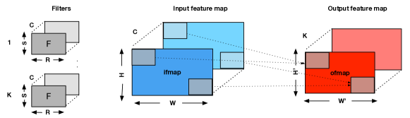
Figure 1. Illustration of a convolution layer along with its inputs.

One method to build a hardware accelerator for CNNs. The sliding-window nature of the convolution operation introduces overlaps between the patches. It makes the job of designing the hardware accelerator challenging because mapping the computation of a convolution operation to a set of processing elements (PEs) is more complex. One commonly used method is to design a fetch unit within each PE that fetches the input patch, communicates the patches with other PEs, and manages the partial results. A specialized interconnect is typically used to facilitate the communication between the PEs based on the specific dataflow. Prior work such as SCNN (Parashar et al., 2017) and Eyeriss (Chen et al., 2017) adopt this approach. The main weakness of this approach is that the interconnection network and dataflow are heavily customized for the convolution operation. Hence, both SCNN and Eyeriss can be inefficient for other layers, such as fully connected layers. For example, SCNN can achieve 25% of the peak throughput when used for the fully connected layers. Similarly, Eyeriss fails to achieve high PE utilization for small batch sizes.

2.2. Transforming Convolution to General Matrix-Matrix Multiplication

The convolution operation can be transformed into general matrix-matrix multiplication (GEMM) using the Im2Col transformation. To structure the convolution operation as matrix multiplication, we need to create two matrices from the two inputs of a convolution layer: input feature map and the K filters. Figure 2 illustrates how the two matrices are built. The product of these two matrices will be equivalent to the result of the convolution operation. For building the weight matrix, each filter is mapped to one row of the weight matrix. When there are K filters, there will be K rows in the weight matrix (see Figure 2(a)). The number of columns in the weight matrix is $R\times S\times C$. In contrast to the weight matrix, a more complex transformation is required to build a 2-D matrix from the original 3-D input feature map. This transformation is called Image to Column (Im2Col). The Im2Col result depends on the kernel size and the stride size, which are the two parameters of the convolution operation. In convolution, each filter slides across different positions in the input feature map. We call all elements in the input feature map covered by the filter as a patch or a tile. Patches are often overlapped with each other when the stride size is less than the filter size. This overlap results in the repetition of the same element of the input feature map in multiple patches. Figure 2(b) and Figure 2(c) illustrates the Im2Col transformation with an example filter of size ($3\times 3\times C$) and a stride of 1. Each column of the matrix produced by the Im2Col transformation corresponds to one patch where the filter is applied for all $C$ channels, and it has $R\times S\times C$ rows. Figure 2 shows the patches for one channel. Finally, the product of the two matrices (Figure 2(a) and 2(c)) generates the output of the convolution operation.

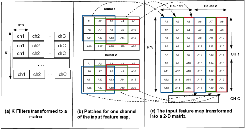
Figure 2. Transforming the inputs of a convolution layer (i.e., input feature map and filters) into two matrices to use a GEMM-based formulation of convolution.

Benefits and challenges of convolution with Im2Col. By using a separate Im2Col transformation, the task of building input patches and the eventual computation on them can be decoupled. The Im2Col transformation can identify data overlap among different patches as each filter slides across different positions in the input feature map. Further, a separate Im2Col transformation can enable one to use highly optimized primitives or even available hardware accelerators for GEMM. However, doing the Im2Col transformation in software may not provide the best possible performance because of redundant accesses with the GEMM computation and increased data storage/communication. The Im2Col transformation can account for as much as 60% of the total execution time of the convolution operation. Figure 3 reports the percentage of the total execution time that is spent in the Im2Col transformation for various layers in AlexNet, VGGNet, and GoogleNet for a CPU system. On average, the Im2Col transformation spends 29% of the overall execution time. Additionally, a naive Im2Col transformation can result in numerous redundant memory accesses. Several repetitions in the Im2Col patches are created by sliding the filters over the input feature map. Depending on the filter size and the stride size, the number of memory access can be $9\times$ higher on average than the number of elements, which indicates that many elements are redundantly accessed multiple times.

Section 3 describes our accelerator that performs Im2Col on-the-fly, extracts significant parallelism between various patches, and use the hardware Im2Col unit to simplify the hardware accelerator for GEMM without the need for complex interconnection networks.

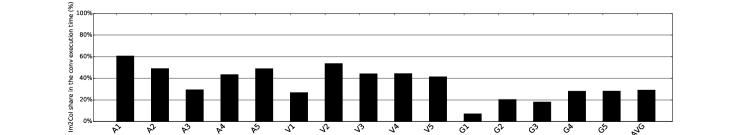
Figure 3. The percentage of the total execution time spent in the Im2Col transformation for various convolution layers from AlexNet, VGGNet, and GoogleNet for a CPU system.

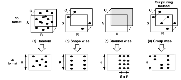
Figure 4. This figure shows the resulting zeros in the 2-D matrix representation of the filter while pruning the filters at different granularities and their corresponding matrix format. A dark dot indicates that the point is being pruned.

2.3. Sparsity-Awareness in CNNs

A fraction of the values in the layers’ weight and feature map are zeros. During training, a pruning step is often applied to remove unimportant and redundant weights, which can result in numerous zeros in the final trained weights. Additionally, some zeros can also appear in the feature map input. Unlike zeros in the weights, these zeros need to be identified at run-time.

The pruned weights can be compressed using a sparse format. In addition to reducing the model size, different hardware accelerators use sparsity at different levels to improve their design’s performance and energy efficiency. The performance improvement comes from eliding multiplications and minimizing data movement when it involves zeros. Next, we review some of the sparsity-awareness techniques and their weaknesses to motivate our proposal.

Techniques for skipping the zeros. SparTen (Gondimalla et al., 2019) and ExTensor (Hegde et al., 2019) add extra hardware to find the matched non-zero values to multiply (i.e., intersect operation). The hardware cost of the intersection operation is high (e.g., a prefix sum for SparTen and content addressable memory for ExTensor). SCNN (Parashar et al., 2017) adopts another approach to avoid zeros in both feature maps and weights by using an outer product. While the SCNN approach successfully removes the costly intersection operation, it introduces redundant multiplications in an effort to handle overlaps in the input tiles.

Unlike these approaches, we avoid the zeros in the input controller. It relieves the PEs from doing extra costly operations (e.g., intersection) and redundant operations. We will explain the details of our sparsity-awareness design in Section 3.3.

Techniques for pruning filters. There are two strategies for pruning: random pruning and structured pruning. The random pruning sets a weight to zero if it is below a threshold value (Han et al., 2016b). Typically after the pruning step, non-zero weights need to be stored in a compressed sparse format. However, using a sparse format involves indirect accesses and requires extra steps for extracting the non-zero elements and matching indices. In contrast, structured pruning address the irregular accesses due to random pruning (Wen et al., 2016; Kung et al., 2019; Kang, 2020). Structured pruning removes redundant weights only at well-defined locations or with specific block sizes.

Figure 4 shows pruning at different levels with various pruning methods. The dark points represent pruned weights in the filter. When we convert a 3-D filter to a 2-D representation using the strategy shown in Figure 2(a), the resulting zeros in the 2-D matrix is shown in the second row of Figure 4. Random pruning results in an irregular pattern of zeros. A coarse-grained structure (e.g., channel-wise) for pruning can result in a group of zero columns in the 2-D matrix, which is more hardware friendly. However, it can sacrifice network accuracy. A fine-grained structure (e.g., shape-wise or group-wise) gets closer to the accuracy of random pruning while having a regular structure with zeros. We will describe the details of our group-wise pruning in Section 4.

3. SPOTS Architecture

(a) Overall architecture of SPOTS

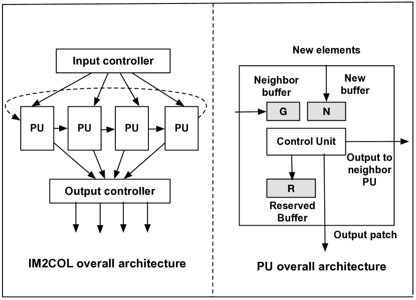
(b) Overall Im2Col architecture and patch unit internals.

Figure 5. (a) The overall architecture of our accelerator with the Im2Col unit and a systolic array-based GEMM unit. (b) The Overall Im2Col architecture and patch unit internals.

We design a hardware accelerator, SPOTS, for the inference phase that provides significant performance and energy benefits for CNNs with different layer characteristics using a GEMM-based formulation of a convolution operation. Our design goals are four-fold: (1) significant performance and energy benefits, (2) support multiple CNN layers and filters of varying sizes, (3) efficient even with sparsity in the weights and the filters, and (4) fine-grained pipelining of the Im2Col operation with the GEMM computation.

We propose a hardware unit for the Im2Col transformation that is synergistic and pipelined with the hardware unit for GEMM. The Im2Col unit reads the input feature map, a 3-D array, and creates a set of linearized patches. The Im2Col unit consists of patch units (PUs) where each PU is responsible for constructing a linear patch. As values are streamed in, the PU constructing the patch will forward overlapped elements to neighboring PUs. Once the PU collects all the values in a patch, it forwards in-order partial patches to the GEMM unit. The approach allows the Im2Col unit to read in values from the input feature map once and reuse them to save redundant memory accesses.

We design a dynamically reconfigurable GEMM unit with a systolic array based design. It can be configured as a tall array to balance the work between Im2Col and GEMM computation. To maintain a high PE utilization with CNN layers with varying shapes, the GEMM units can be configured as small GEMM units (see Section 3.4). This dynamic reconfigurability enables our hardware to adapt to CNN layers with varying dimensions and shapes. Further, it also helps with sparsity-awareness by enabling our design to detect and skip zeros in the input feature map (see Section 3.3). Figure 5(a) shows the overall architecture of our accelerator. The two main components are the unit for the Im2Col transformation and the GEMM unit. They are connected by two buffers that allow effective pipelining of the operations between the Im2Col unit and the GEMM unit.

3.1. The Im2Col Unit

The Im2Col transformation creates a 2-D matrix from the 3-D input feature map, which reduces convolution to matrix multiplication (See Section 2.2). The Im2Col transformation is challenging because it inherits a part of the complexity of convolution, has complex memory access patterns, and results in redundant accesses. We propose a distributed hardware structure consisting of a series of Patch Units (PUs) to both accelerate Im2Col and minimize the number of accesses to the elements of the input feature map. The key insight in our Im2Col unit is to exploit the localities resulting from the overlap between the patches as we slide the filters across the input feature map both vertically and horizontally. Each PU is responsible for building one patch at a time. One of our design goals is to read the input feature map only once from SRAM. To accomplish this goal, each patch unit has small local buffers that store some values that will be useful for building future patches. The PUs are also connected using a ring network, which allows the PUs to communicate elements locally and avoid redundant accesses to the input feature map in SRAM. Figure 5(b) shows the overall architecture of our Im2Col unit that consists of three main components: input controller, PUs, and output controller. The input controller reads the input feature map from SRAM and forwards them to the appropriate PU units. Apart from sending values from the input feature map to the respective PUs, the input controller maintains extra metadata for every scheduled patch. This metadata carries information about the position of the current patch. For some convolution layers, stride size is the same as kernel size. In those cases, there is no overlap between the patches. For those scenarios, the input control forwards its output directly to the output controller by skipping the PUs.

Our Im2Col unit has multiple PUs within it. The PUs are the main components of the Im2Col unit for generating patches. Figure 5(b) shows the internals of the PU. Each PU has three buffers: the new buffer, the neighbor buffer, and the reserved buffer. The new buffer (N) maintains the newly fetched element received from the input controller. The neighbor buffer (G) stores the elements received from the neighboring PU. The reserved buffer (R) stores some of the elements previously received at that PU in the previous rounds. We store the row and column indices (i.e., coordinates) along with the value for each element. The control unit within each PU manages the buffer and generates patches. It decides whether an element needs to be forwarded to the neighboring PU and whether it should be maintained in the reserve buffer for future use.

A unique identifier identifies each patch (i.e., row and column index of top-left element). The control unit in a PU uses the patch identifier, the filter size, and the stride size to determine which elements need to be (1) fetched from the input feature map, (2) forwarded to the neighboring PUs, and (3) stored in the reserve buffer for future rounds. For example, all elements need to be fetched from the input feature map when a PU processes the first patch in the first round.

All elements that are necessary for adjacent patches in a given round are provided by the neighboring PUs. A PU typically receives $K^{2}-K\times S$ elements from the neighboring patches as long as it is not the first patch in a given round, where $K$ is the size of the kernel and $S$ is the stride size. We assign all patches that belong to the same column (i.e., column index of the top-left element) in different rounds to the same PU. Hence, the PUs also stores some elements that may be useful to build patches in subsequent rounds in the reserved buffer. This procedure is repeated for all C channels in the feature map.

The total number of elements that are overlapped between the vertical patches for a given filter size is $C\times W\times\left(K-S\right)$ where $W$ is the width of the input feature map. This is the maximum data reuse that can be attained with the reserve buffer. Further, the width and the channel size are inversely proportional to each other. For example, the first few layers of a CNN often have a small number of channels that are wider. In contrast, the later layers of the CNN have larger channels of smaller width. Thus, a small reserve buffer can provide significant data reuse even for larger layers. When the number of overlapped elements between the vertical patches is larger than the size of the reserved buffer, the input controller skips the reserved buffer and fetches the element again from SRAM. In such cases, data reuse is restricted to horizontally adjacent patches. Finally, the output controller organizes patches formed by each PU and manages communications with the GEMM unit. It coordinates double buffering that enables the overlapped execution of the Im2Col unit and the GEMM unit.

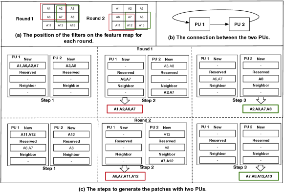
Figure 6. Illustration of patch generation using the PUs in the Im2Col unit. We show an Im2Col unit with 2 PUs for exposition. (a) The input feature map with one channel. We show the sliding windows used to generate patches with a stride of 1. (b) The two PUs are interconnected by a ring network. (c) There are two rounds. Round 1 corresponds to patches belonging to the first row of sliding windows over the input feature map. Similarly, round 2 corresponds to patches belonging to the second row of sliding windows.

Figure 6 illustrates the process of generating the patches using the PUs in our Im2Col unit. For example, PU1 receives four elements (A1, A6, A2, A7) from the input controller and stores them in the new buffer in step 1. Similarly, PU2 receives two new elements (A3, A8). PU2 will receive other elements from the PU1 in subsequent steps (i.e., step 2).

In summary, our hardware Im2Col unit provides two benefits: energy efficiency and performance. Accessing the smaller SRAM and performing integer operations (for computing on row and column indices) consumes significantly less energy than accessing DRAM and large SRAMs. Hence, our design provides significant energy benefits. Further, our distributed collection of PUs unlocks extra parallelism beyond parallelism among the channels, allowing multiple patches to be built simultaneously by different PUs in the Im2Col unit that boosts performance.

3.2. The GEMM Unit

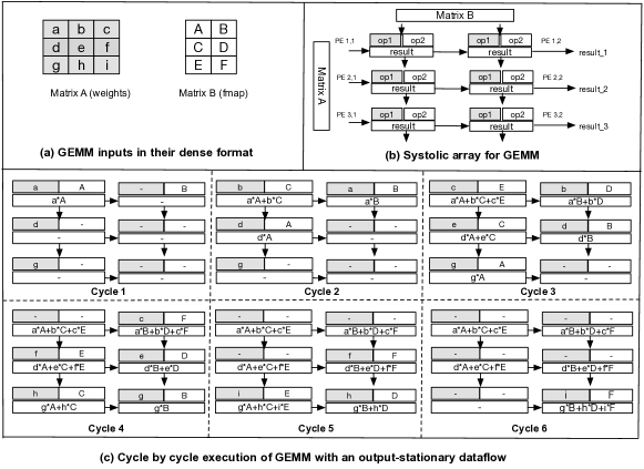
Figure 7. Illustration of our GEMM unit. (a) Inputs to the GEMM unit. (b) A tall array for the GEMM unit. (c) Illustration of GEMM computation at various steps. We show the current inputs and the partial results computed till a step for each PE. We demonstrate the output-stationary attribute of our design.

Our hardware unit for accelerating GEMM is a systolic array-based design. Unlike many prior proposals that use systolic arrays for GEMM (Chen et al., 2017; Kung et al., 2019; Jouppi et al., 2017; Kwon et al., 2019b; Kung et al., 2019), we add dynamic reconfigurability to the GEMM unit. The GEMM unit in SPOTS can be configured either as a tall shaped systolic array (the height is considerably larger than the width) to maximize data reuse or as multiple GEMM units with square shaped systolic arrays. Figure 7(b) shows our systolic array-based design for GEMM with a tall array.

There are two main benefits in using a tall-shape systolic array-based architecture for GEMM. First, one of the inputs of the GEMM unit comes from the Im2Col unit. Using a tall shape array reduces the memory bandwidth requirement for the input arriving from the Im2Col unit. Thus, we can attain high PE utilization in the GEMM unit with less throughput from the Im2Col unit. This helps us to build an Im2Col unit with fewer resources and memory bandwidth requirements. Second, the tall array helps our design to exploit sparsity in the output of the Im2Col unit to skip zeros and increase performance. As the width of the tall array is smaller than its height, fewer columns from the Im2Col transformation enter the systolic array at any instant of time, which increases the opportunity for detecting and skipping entire rows of inputs with zeros before entering the systolic array. In essence, using a tall-shape array helps to simplify our mechanism to skip the redundant computation involving zeros in the input feature map. We will explain our sparsity-awareness approach later (See Section 3.3). Dynamic reconfigurability enables it to be reorganized as multiple GEMM units for a few instances where a tall-shape array is not suitable to keep all the PEs utilized (see Section 3.4).

Our GEMM unit uses an output-stationary dataflow where a given processing element (PE) computes the final result by accumulating the partial products for a particular element of the output. This output-stationary dataflow ensures maximum reuse of the output data. Using a tall array also helps us attain high data reuse for the result of the Im2Col transformation. Figure 7(a) shows the weight matrix from the filter and the output of the Im2Col transformation that forms the input to the GEMM unit. The values of the filter matrix enter the GEMM unit’s systolic array from left-to-right. While the result of the Im2Col unit enters the systolic array from top-to-bottom. Figure 7(c) shows the various steps and partial results computed in the GEMM unit. Our design is parameterizable with $M$ rows and $N$ columns in the systolic array. In our design, each row handles multiple rows of the filter matrix. Our specific prototype used 128 rows of PEs and 4 columns. These numbers are chosen based on the characteristic of common CNN layers. Further, each row of the systolic array can be assigned multiple rows of the filter matrix depending on the scheduling mode. The majority of layers in state-of-the-art CNNs have less than 512 rows of the filter matrix in each convolution layer.

Each PE has a single multiply-accumulate (MAC) unit that uses two 16-bit fixed-point inputs and accumulates the result in a 24-bit register. To handle multiple rows of the filter matrix, each PE has $K$ registers to compute the final result (e.g., in our design, we use $K=4$). Each PE has three FIFOs. Two FIFOs, one for each arriving inputs. The other FIFO works as the work queue for the MAC unit. In GEMM, the coordinates of the elements of the two input matrices should match before multiplying the inputs. In the fetch unit, we ensure that the inputs are sent to the PEs in the proper order; thus, we do not need additional logic to perform index matching inside a PE. Additionally, our output-stationary dataflow ensures all the partial products produced in a PE belongs to the same output element. Next, we describe how to support sparsities in both inputs without requiring any index matching units inside the PEs.

3.3. Handling Sparsity in CNNs

Most CNNs have sparsity in both filters and the input feature map. Figure 11 quantifies the amount of sparsity (percentage of the zeros in the total number of elements) for the commonly used CNNs. We use structured sparsity learning (SSL) (Wen et al., 2016) as our pruning method that is further enhanced with optimizations to better suit our hardware design (see Section 4). To support sparsity during inference, we propose a custom sparse format to store the filters pruned with our method and design an approach that identifies a block of entries with all zeros in the result of the Im2Col transformation on-the-fly. These techniques enable our accelerator to skip rows and columns with all zeros before entering the systolic array of the GEMM unit without requiring extra costly hardware for intersection or introducing any redundant zeros (See Section 2.3). Further, they also allow us to gate the MAC units when an operand is zero. As our designs use a tall systolic array and an output-stationary dataflow, these techniques provide high bandwidth access to the filters necessary to keep the PEs active.

Our sparse format for filters. Once the weights for the filters are learned during the training phase, we divide the weights into blocks. The block size is equal to the group size used for pruning, which is a design parameter. Logically, the filter matrix will be 2-D matrix of blocks when viewed in the dense representation. To minimize the memory footprint for storing the filters during the inference, we convert them into a sparse representation that is aware of the number of SRAM banks in the design. Our sparse format uses three arrays to store the pruned weights compactly. Figure 9(a) shows our custom sparse format. We store all non-zero blocks separately in one array (Array A) that is distributed in multiple banks based on the row index of the block (i.e., vertical position in the filter matrix). We use two bitmap arrays M1 and M2 to store the metadata. The bitmap array M1 encodes whether a column has any non-zeros in the filter matrix. A zero in the bitmap array M1 indicates an empty column. The bitmap array M2 maintains whether a block in a non-zero column is non-zero. A zero in M2 indicates the corresponding block is zero (i.e., as a block is a collection of values, it implies that all values in the block are zeros). These three arrays of our sparse format (i.e., A, M1, and M2) are distributed across the various banks of the SRAM so that the input controller for the GEMM unit can access them in parallel. Figure 8 compares the memory footprint of our sparse format in contrast to traditional compressed sparse row format and other sparse formats used in prior work. In contrast to them, our sparse format reduces the memory footprint significantly.

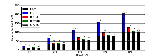
Figure 8. Comparing our custom sparse format with other state-of-the-art sparse formats. We used a matrix with 1632 rows and 36548 columns. We assume the values are 2 bytes. The last bar shows our sparse format. Our sparse format is independent of the density of the zeros in the matrix, and the size of metadata is less than 1 MB across all the density ratios. We compare our sparse format with CSR, RLC-4, and Bitmap in the following order. The size of the sparse metadata is shown at the top of each bar in Megabytes.

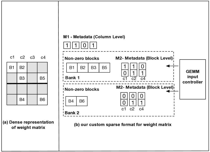
(a) Our custom sparse format to store filters

(b) Skip rows and columns with all zeros

Figure 9. (a) Our custom sparse format to store filters. (b) Illustration of how our design skips rows and columns with all zeros. (1) Weight matrix with the metadata about columns with all zeros. (2) The Im2Col result with the metadata about rows with all zeros. (3) If a row or a column is all zeros, all such rows and columns can be skipped (i.e., and operation of the row and column metadata). (4) GEMM computation when rows and columns are skipped. For example, the first element of column C4 will be fetched by the first PE in cycle 2 (skipping columns C2 and C3).

Handling sparsity in the result of the Im2Col transformation. The compress component before the GEMM unit in our accelerator (see Figure 5(a)) identifies a block of zeros in the result of the Im2Col transformation. It creates a bitmap for every block coming out of the Im2Col unit. If all elements in a block in the output of the Im2Col unit are zeros, the bit is set to zero for that block; otherwise, the bit set to one. Subsequently, the input controller of the GEMM unit uses this bitmap to skip blocks with all zeros on-the-fly. We can elide MAC operations when an operand is zero even before entering the systolic array. Further, it is not necessary to stream the column of filters when one detects such a block of zeros. Figure 9(b) illustrates how the zero columns in the weight matrix and the zero rows in the output of the Im2Col unit are skipped. The $\star$ marker in Figure 11 indicates the percentage of zeros in the output of the Im2Col transformation that is skipped on-the-fly with this technique. We further reduce energy by gating the MAC units when an operand is zero.

3.4. Handling Various CNN Layers/Shapes

Figure 10. (a) Enhancements to reorganize the tall systolic array (SA) as multiple GEMM units. (b) Illustration of how inputs are distributed in the configuration with multiple GEMM units.

CNNs have multiple layers that can be of different shapes and sizes. With a fixed configuration of hardware PEs, they can be underutilized for some layers, shapes and/or sizes. Each filter forms a row of the weight matrix that is assigned to a distinct row of the systolic array. When the GEMM unit is configured as a tall systolic array, and the number of filters is relatively smaller than the systolic array’s height (e.g., 128), some PEs will remain unused.

Dynamic reconfigurability of the GEMM unit enables us to support CNN layers with different attributes (see Figure 10). Specifically, the PEs in the GEMM unit can be configured either as one tall array or multiple small arrays. Each such configuration has the same number of columns. This enhancement allows our design to be more adaptive to different layer shapes and thus maintains high PE utilization under different conditions. Figure 10 (a) demonstrates how a tall array can be used as two smaller arrays using the multiplexers. Hence, the PEs now can receive the input either from the PEs above (i.e., it forms a tall array) or can get the input from a different Im2Col unit. These multiplexers can be configured based on the mode register dynamically depending on the structure of a layer. The weight matrix is broadcast to all small systolic arrays when the GEMM unit is configured as smaller systolic arrays. Each small GEMM unit receives the feature map input from their assigned Im2Col units. The two GEMM units compute two independent groups of columns of the final result matrix (i.e., GEMM 1 computes result columns from 0 to N/2, GEMM computes the columns from N/2+1 to N). In our prototype, we have four Im2Col units. The main Im2Col unit is used when the GEMM unit is used in the tall array configuration. Other Im2Col units are smaller in size to reduce the overall area. This dynamic reorganization of the GEMM unit’s systolic array coupled with the multiple Im2Col units enables our hardware to maintain high PE utilization for various CNN layers with different shapes.

Supporting fully connected layers. Most CNNs have one or more fully connected layers at the end of the network. The inputs to the fully connected layers are the matrix weights learned during the inference and the output feature map resulting from the final pooling or convolutional layer that is flattened to a vector. With a batch size of 1, the computation for a fully connected layer is equivalent to matrix-vector multiplication. By increasing the batch size, we can structure it as a matrix-matrix multiplication operation. As we use a tall array, the batch sizes need not be large to utilize the whole array of PEs fully (e.g., can be as small as 4).

Supporting pooling layers. The pooling layers help to summarize the features generated by a convolution layer. There are two common types of pooling layers: max pooling and average pooling. Among them, max pooling, which picks the maximum element from a feature covered by the filter, is more common. Similar to convolution layers, the pooling layer has two parameters, filter size and the stride size. We support the pooling layer by adding the pooling operation (e.g., MAX) to the output of the patch units (PUs) in the Im2Col unit.

4. EXPERIMENTAL METHODOLOGY

Table 1. SPOTS design parameters and area.

. Unit Size Area (mm2) #PE units 512 Multiplier width 16 bits GEMM Accumulator width 24 bits 2.048 Systolic array one (128$\times$4) configurations four (32$\times$4) PE’s local buffers 2 KB #PU units 4 Im2Col Reserved buffers 32 KB 1.137 Other SRAM buffers 2 MB On-chip Filter SRAM 1 MB 5.426 memory Fmap SRAM 512 KB SPOTS total 8.611

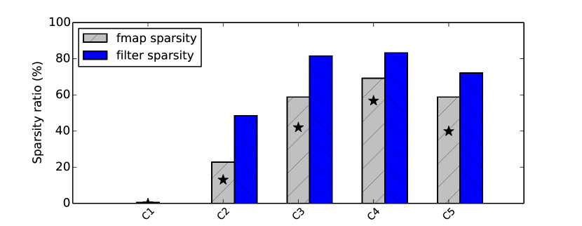
(a) AlexNet.

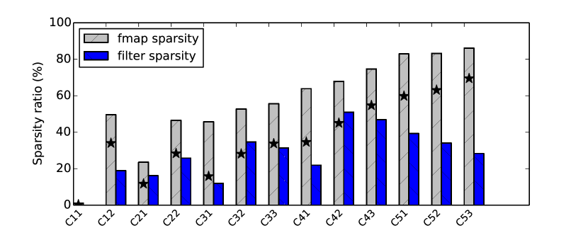
(b) VGGNet.

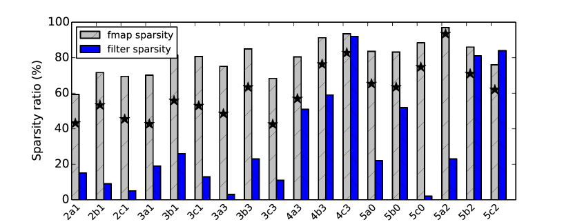
(c) ResNet.

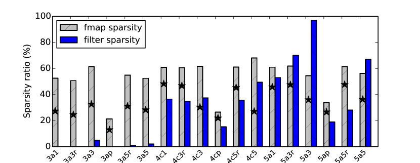
(d) GoogleNet.

Figure 11. Sparsity in the filters and input feature maps for AlexNet, VGGNet, ResNet, and GoogleNet. The $\star$ marker indicates the percentage of zeros in the output of the Im2Col transformation that is skipped on-the-fly by our design.

We built a prototype of our design in Verilog and synthesized it using Synopsys Design Compiler with FreePDK 45nmcm technology (Stine et al., 2007). Our design achieves a maximum of 500 MHz frequency. FreePDK 45 does not include SRAM cells. Thus, we separately model the area and power of all the SRAM/DRAM using Cacti 7.0 (Balasubramonian et al., 2017). Table 1 provides the parameters of the SPOTS prototype and the area breakdown for different components. We perform a cycle-accurate simulation of the RTL model of SPOTS in Verilog using Verilator. We used the traces from our RTL simulation and estimated the power consumption of our design with Synopsys’s PowerPrime tool. During our simulation, we executed each layer at a time. The pruned weights are preprocessed and are provided in our proposed sparse format. For the input feature map, we extracted each layer’s data from the models in Caffe. We also developed additional infrastructure to perform fast design space exploration and to collect statistics.

CPUs, GPUs, and other ASICs used for our evaluation. We compare our prototypes with CPUs, GPUs, and other ASICs. We use Caffe to evaluate various CNN architectures on a modern CPU and GPU. The details of the CPU and GPU that we use for the evaluation is shown in Table 3. The CPU and GPU we used in our experiments are manufactured with 22 nm and 16 nm cell technology, compared to 45 nm technology used for SPOTS. The Caffe framework uses IntelMKL for CPU computation and Nvidia’s CUDA library, cuSparse, for the GPU computation. Similar to our design, Caffe adopts a Im2Col + GEMM approach for doing convolution layers. We measured the energy consumption of the XEON CPU using Processor Counter Monitor (PCM) (int, [n. d.]). For GPU, we measured the power consumption with NVIDIA System Management Interface (Nvidia-smi) (nvi, [n. d.]) that queries the power using the built-in sensors. According to NVIDIA, the reported data is accurate (i.e., within $\pm$ 5 Watt).

Table 2. Network characteristics and their the top1 and top5 result accuracy for the pruned and the original model. Weights and activations assume a data-type size of two bytes.

Model	#conv	Max. Layer	Max.	Median	Median	Dataset	Baseline(%)	Our Pruning (%)
	Layer	Feature map	Layer	Kernel	Stride		Top1/Top5 Acc	Top1/Top5 Acc
			Weight	Size	Size
AlexNet (Krizhevsky et al., 2017)	5	0.3 MB	2.5 MB	3	1	Imagenet	56.81/79.95	55.25/78.62
VGGNet (Simonyan and Zisserman, 2015)	13	6.1 MB	4.5 MB	3	1	Imagenet	68.27/88.36	67.18/88.16
GoogleNet (Szegedy et al., 2015)	57	0.36 MB	1.3 MB	1	1	Imagenet	68.92/89.14	66.22/87.53
ResNet (He et al., 2016)	53	1.5 MB	4.5 MB	1	1	Imagenet	77.71/90.66	69.71/89.30

Table 3. The CPU and GPU configurations.

Platform	Number of cores	Frequency	Main memory	Technology node	Cache
Intel Xeon E5-V3	4	3 GHz	32 GB DDR4	22nm	10 MB
			(2666 Mhz)		Smart Cache
Titan X Pascal	3584	1.53 GHz	24 GB of GDDR5	16nm	-
			(peak bandwdith 480 GB/S)

Eyeriss. Although there are many prior ASICs on accelerating CNN networks, most of them report relative performance numbers, and their designs are not publicly available. We use Eyeriss (Chen et al., 2017, 2016), which is an ASIC designed for accelerating sparse CNNs, to compare against our design. Eyeriss uses a row-stationary (RS) dataflow to maximize data reuse and minimize expensive data movements. Further, data compression and data gating techniques are applied to improve energy efficiency. Eyeriss chip (Chen et al., 2017) is composed of 168 Processing Elements (PEs) structured as a $12\times 14$ array. The PEs are connected with a network-on-chip (NOC) that enables multicast and point-to-point single-cycle data delivery to support the RS dataflow. We measure the performance of Eyeriss using the publicly available simulator (Gao et al., 2019). Eyeriss chip is fabricated at 65 nm CMOS and operates at 200 MHz clock frequency. Since we used a different cell technology (i.e., 45 nm) for SPOTS, we assume that the frequency of Eyeriss to be exactly equal to the frequency of SPOTS when we report the execution time. We also configured Eyeriss to use the same number of MAC units and on-chip memory as SPOTS. Additionally, both SPOTS and Eyeriss designs use 16-bit fixed-point inputs.

Gemmini is a recent open-source full-stack DNN accelerator generator. Gemmini (Genc et al., 2021) can be used to explore the design-space of efficient DNN accelerators. The core unit in Gemmini is a systolic array composed of processing elements (PEs). Each PE can perform dot products and accumulations. The PEs reads the data from local, explicitly managed scratch-pad of banked SRAMs. Gemmini uses a two-level hierarchy, first composed of tiles, where tiles are connected via explicit pipeline registers. Each tile can be further broken down into an array of PEs. Most design parameters can be adjusted to explore various designs. We failed to build a design with an exact total number of PEs as SPOTS. Thus, we used tiles with $32\times 32$ PEs for Gemmini, which translates to a total of 1024 MAC units, which is 2$\times$ more MAC units than our prototype. We also set the scratch-pad and banking size parameters in Gemmini to match the on-chip memory used for SPOTS. Like our approach for measuring the cycle counts, Gemmini’s simulator reports the cycle counts from simulating the design with Verilator.

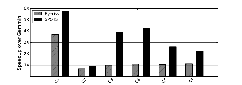
(a) AlexNet

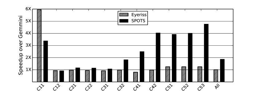
(b) VGGNet

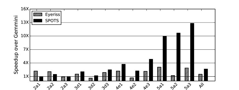
(c) ResNet

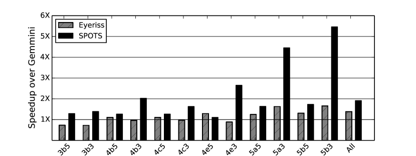
(d) GoogleNet

Figure 12. Speedup with SPOTS and Eyeriss over Gemmini for four CNNs: AlexNet, VGGNet, ResNet, and GoogleNet. The figures show the speedup for selected layers from the top, middle, and bottom layers and the overall speedup (the last bar in each figure).

CNN architectures and pruning. We used four widely used CNN architectures: AlexNet (Krizhevsky et al., 2017), VGGNet-16 (Simonyan and Zisserman, 2015), GoogleNet (Szegedy et al., 2015), and Resnet-50 (He et al., 2016) to evaluate our prototype. We refer to VGGNet-16 and ResNet-50 as VGGNet and ResNet, respectively, throughout the paper. These four CNN architectures vary in the number of layers, layer types, and sizes, as Table 2 presents. We used a batch size of one for all of our experiments, which is the standard usage mode for an inference task. We used the input images from the Imagenet (Deng et al., 2009), a widely used dataset for image classification tasks, to train the networks. We pruned all four networks using the pruning algorithm based on Structure Sparsity Learning (SSL) (Wen et al., 2016). SSL is generic and can be applied in different levels, including filters, channels, and shapes. We applied SSL at the shape level. As our hardware exploits sparsity at a much finer granularity than a shape, we optimize SSL by pruning in a more fine-grained fashion. Specifically, we zeroed the weights that are below the threshold in some but not all elements of a shape. This generates zero blocks of a certain size (i.e., the number of filters in the group). Figure 4(d) shows our group-wise pruning. Figure 11 reports the sparsity in the weights and input feature map after pruning for the layers of various CNN architectures. It shows that sparsity varies across both layers and networks. Finally, we retrained the pruned network to regain its accuracy, which is the norm with pruning. Table 2 reports the top-1 (i.e., the first prediction is the correct result) and top-5 (i.e., the correct result is in the first 5 predicted values) accuracies of the pruned network and the original network. Our pruned networks are within 1%-2% accuracy of the original model without pruning.

5. Experimental Evaluation

We demonstrate the performance and energy efficiency of SPOTS in comparison to Eyeriss, Gemmini, CPU, and GPU implementations.

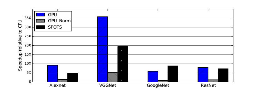
(a) Speedup with SPOTS

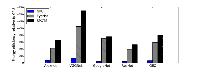
(b) Energy efficiency with SPOTS

Figure 13. (a) Speedup with SPOTS, GPU, and GPU implementations with the normalized number of MAC units over the CPU implementation as the baseline. (b) The energy efficiency of SPOTS and GPU implementations compared to a CPU baseline.

Performance of SPOTS when compared to Eyeriss and Gemmini. Figure 12 reports the speedup of SPOTS and Eyeriss relative to Gemmini for all four CNN architectures. The layers are sorted for each CNN architecture based on where they appear in the network (top, middle, or bottom). Figure 12(a) reports the speedup for all layers in AlexNet. On average, SPOTS is almost 2$\times$ faster than Eyeriss and Gemmini. SPOTS is nearly $4\times$ faster than Eyeriss and Gemmini for the layers in the middle, where the sparsity ratio in the two inputs (e.g., weights and feature map) is higher. In addition to the sparsity awareness that gives SPOTS an advantage over Eyeriss and Gemmini, the layers in the middle and bottoms have more filters that favor a tall systolic array.

Figure 12(b) reports the speedup for VGGNet. On average, SPOTS is $1.85\times$ and $1.86\times$ faster than Eyeriss and Gemmini, respectively. Similar to AlexNet, SPOTS achieves higher speedup with layers with more sparsity. SPOTS perform slightly worse than Eyeriss for the first two layers, where the number of filters is relatively small, and the inputs are dense (See Figure fig:sparsity). Later in this section, we will demonstrate the connection between the number of filters in a layer and the PE utilization. Figure 12(c) shows the speedup of SPOTS over Eyeriss and Gemmini for ResNet. SPOTS is 1.77$\times$ and 2.66$\times$ faster than Eyeriss and Gemmini on average for ResNet. SPOTS is up to 8$\times$ and 13$\times$ faster than Eyeriss and Gemmini for the layers where the weight and feature map sparsity is high. Similar to VGGNet, SPOTS performs slightly worse or similar to Eyeriss for the first eight layers in ResNet because the first few layers in ResNet have a few filters per each layer. Hence, PEs are underutilized compared to layers in the middle or at the end of the network. Figure 12(d) shows for GoogleNet, SPOTS is 1.38$\times$ and 1.91$\times$ faster than Eyeriss and Gemmini, respectively. In contrast to other CNN architectures, GoogleNet has a few convolutional layers at the beginning with a small number of filters that do not favor our tall array. Thus, overall, SPOTS enjoys less speedup for GoogleNet compared to the three other networks.

Performance comparison with CPUs and GPUs. We evaluate the performance and energy efficiency of SPOTS in comparison to execution with CPUs and GPUs. Figure 13(a) reports the speedup of SPOTS for the convolution layers over the CPU implementation. SPOTS has 5$\times$, 20$\times$, 6$\times$ and 8$\times$ speedup over the CPU implementations using Intel MKL for AlexNet, VGGNet, GoogleNet, and ResNet, respectively. SPOTS attains this speedup while operating at a frequency almost 6$\times$ less than the CPU. Figure 13(a) also shows the speedup of GPUs for the convolution layers over the CPU implementation. Compared to GPUs, SPOTS is about 2$\times$ slower than GPU for AlexNet and VGGNet, while performs slightly better or similar to GPU for GoogleNet and ResNet. VGGNet and AlexNet layers are relatively larger than the other two networks, resulting in larger matrices that favor the GPU with abundant MAC units compared to SPOTS. The second bar Figure 13(a))(a) shows the GPU performance when its number of MAC units is normalized to the number of MAC units in SPOTS. For the normalized number of MAC units, SPOTS outperforms the GPU on average by 6$\times$. Finally, some prior work observed that the performance degrades for CPUs and GPUs when the sparse features are used when the networks are pruned randomly. However, we observed that using our structured pruning helps the CPU and GPU implementations to attain higher overall performance using sparse linear algebra kernels.

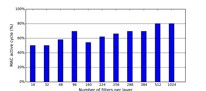
(a) MAC utilization

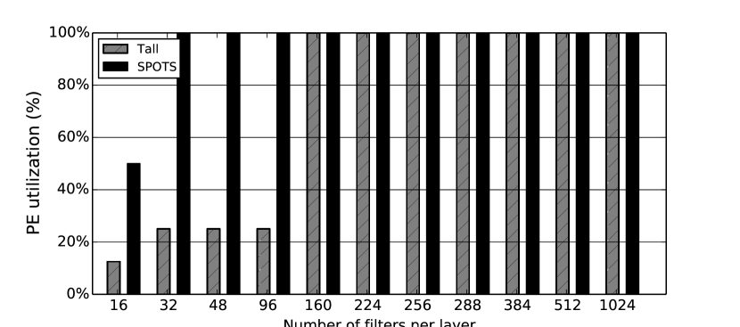
(b) PE utilization

Figure 14. (a) MAC utilization (i.e., active cycles) for different filter sizes. (b) Comparing PE utilization of SPOTS and Tall systolic array (i.e., active PEs) for different filter sizes.

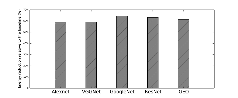
(a) Im2Col energy efficiency

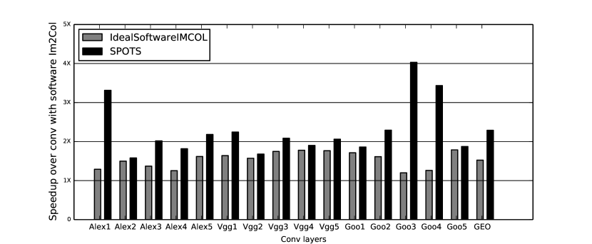
(b) Hardware Vs. Software Im2Col

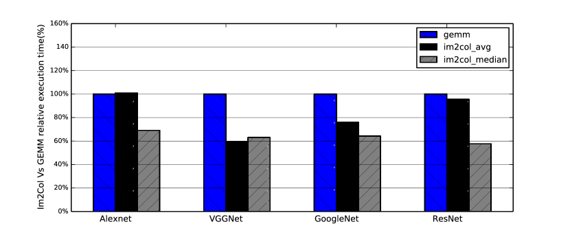
(c) Im2Col Vs. GEMM

Figure 15. (a) The reduction in energy consumption for the Im2Col unit of SPOTS over the baseline design. (b) Speedup with SPOTS over the software-based Im2Col as the baseline Im2Col design with no data reuse. (c) Fraction of the work performed by the Im2Col unit when compared to GEMM (i.e., GEMM bar is 100%). We report the average and the median for the Im2Col’s work. When the mean exceeds the median, there will be instances where the Im2Col does more work compared to GEMM for some layers.

Energy efficiency compared to CPUs and GPUs. Figure 13(b) demonstrates the energy efficiency of SPOTS and GPU implementations when compared to a CPU baseline for four CNNs. We did not include Gemmini energy results since their tool does not report the power consumption. The energy results include the off-chip memory accesses in this data. Our accelerator consumes 78$\times$, 12$\times$, and 1.4$\times$ lesser energy than a CPU, a GPU, and Eyeriss, respectively.

Sensitivity to shapes of various layers. Widely used CNN networks vary in the depth and the number of filters used in each layer. Even within a CNN, the layer shape and filter sizes can vary significantly. The dynamic reconfigurability in SPOTS provides flexibility to use the GEMM unit as a tall systolic array or as multiple small systolic arrays, which allows it to adapt to various shapes and filter sizes. When the filters are small (e.g., less than 128), the GEMM unit is configured as multiple small systolic arrays, which use different Im2Col units. All the PEs in the systolic array are active 100% of the time for all filter sizes other than 16 (See Figure 14(b)). In contrast, a tall systolic array without the enhancement we proposed in Section 3.4 fails to achieve full PE utilization for smaller filter sizes, as Figure 14(b) shows. Figure 14(a) shows the utilization of the multiply-accumulate units in the PEs of the systolic array (i.e., active cycles) when the layer has a specified number of filters (i.e., x-axis reports the size of the filter). When the filter size increases, we assign more rows to a PE, which can fetch up to four elements per read operation. Hence, there are more opportunities to keep the multiply-accumulate units in the PE active (i.e., almost 80% active cycles).

Amount of work performed by Im2Col and GEMM units in SPOTS. As the Im2Col and the GEMM units are pipelined in SPOTS, ideally, the work done by the Im2Col unit and the GEMM unit should be balanced. Figure 15(c) shows the relative percentage of cycles where the Im2Col and GEMM units are active relative to the GEMM unit for the four CNN architectures. As we report the active cycles relative to the GEMM unit, the bar for the GEMM unit is 100%. The average work performed by the Im2Col unit and the GEMM unit are almost similar for AlexNet and ResNet (i.e., the work is balanced). In contrast, GEMM dominates the total work in VGGNet. This data suggests that adding more PE’s to the GEMM unit may improve the overall execution time for VGGNet. As the Im2Col unit is inactive due to low bandwidth with AlexNet and ResNet, adding more PEs without increasing the bandwidth will not improve performance.

Energy efficiency from data reuse in the Im2Col unit. One of the key idea in the Im2Col’s patch unit is to read the input feature map only once from the SRAM and reuse the data with the help of local buffers. Figure 15(a) reports the percentage decrease in energy consumed by using local buffers to reuse the data in the patch units compared to a naive version of Im2Col that access SRAMs multiple times without any data reuse. On average, the mechanisms that we added to reuse the input feature map in the patch units result in the Im2Col unit consuming 60% less energy when compared to the Im2Col unit without such reuse.

Comparing SPOTS with software Im2Col. SPOTS has a hardware Im2Col unit that performs the Im2Col transformation on-the-fly. Figure 15(b) compares the speedup of using a hardware Im2Col unit compared to a software-based Im2Col as the baseline. For the baseline system, the hardware only performs GEMM while the CPU executes the Im2Col. The figure also shows the ideal situation for a software-based Im2Col design where the software Im2Col and the hardware GEMM computations are overlapped. Even when we provide an ideal scenario for the software Im2Col, SPOTS outperforms the ideal software-based Im2Col. On average, SPOTS outperforms the baseline software Im2Col by 2.3$\times$, which shows the benefits of our hardware Im2Col unit.

6. Related work

Table 4. Qualitative comparison of SPOTS with prior work.

Accelerator	Supports sparsity				Supports	Adaptive to
	Feature map	Weight	Gate zero	Skip zero	pruned network	different layer
						shapes
Eyeriss (Chen et al., 2017)	✓	✗	✓	✗	✗	✗
Cnvlutin (Albericio et al., 2016)	✓	✗	✓	✓	✗	✗
CambriconS (Zhou et al., 2018)	✓	✓	✗	✓	✓(structured)	✗
SCNN (Parashar et al., 2017)	✓	✓	✓	✓	✓(random)	✗
CMSA (Xu et al., 2021)	✗	✗	✗	✗	✗(random)	✓
Column comb. (Kung et al., 2019)	✗	✓	✗	✓	✓(structured)	✗
SIGMA (Qin et al., 2020)	✓	✓	✗	✓	✓(random)	✓
SPOTS (this work)	✓	✓	✓	✓	✓structured	✓

There is a large body of literature on using custom hardware accelerators to improve the performance and energy efficiency of neural networks (Albericio et al., 2016; Zhang et al., 2016; Parashar et al., 2017; Chen et al., 2017; Reagen et al., 2016; Chen et al., 2014; Han et al., 2016a; Sharify et al., 2019; Albericio et al., 2017; Chen et al., 2014; Sharma et al., 2016; Huang et al., 2019; Deng et al., 2021; Genc et al., 2021). Table 4 qualitatively compares SPOTS with more closely related work. The table shows that SPOTS supports various operations in CNNs, is adaptive to different layers’ shapes to keep the PE’s utilization high for different scenarios, and efficiently handles sparsity in both feature map and weights.

Support for sparse inputs. Prior work has improved energy efficiency by supporting sparse inputs during inference. Cnvlutin (Albericio et al., 2016) exploits sparsity in the input feature map to skip multiplication operations and to avoid data movement with zero elements. CambriconX (Zhang et al., 2016) supports sparsity in the weights. Similar to our work, SCNN (Parashar et al., 2017) and CambriconS (Zhou et al., 2018) support sparsity in both the feature map and the weights to improve energy efficiency and performance. Prior work also uses data gating techniques to reduce the power consumption when the operands are zeros (Reagen et al., 2016; Chen et al., 2017). While this technique is effective in reducing power consumption, it does not reduce the number of effective operations. Similar to SPOTS, prior hardware designs have developed techniques to skip zeros and to minimize data transfer (Han et al., 2016a; Parashar et al., 2017; Mo et al., 2020).

Support for various layers in CNNs. Often, hardware designs are customized for one type of computation and do not support all types of layers in CNNs, such as pooling layers (Kung et al., 2019; Asgari et al., 2019). EIE (Han et al., 2016a) is intended for the fully connected layers in CNNs. It stores the input feature map and filters in a compressed format and passes only non-zero operands to the multipliers. In contrast, SCNN (Parashar et al., 2017) and Eyeriss (Chen et al., 2017, 2016) primarily focus on the convolution layers. Hence, they can underperform for the fully-connected layers. SCNN can achieve 25% of peak throughput when performing the fully connected CNN layers. Similarly, Eyeriss provides significant energy gains only when batch sizes are larger than 16. In contrast, SPOTS supports all the common layers that exist in CNNs.

Systolic array designs for CNNs. Recent work (Kung et al., 2019; He et al., 2020) uses a preprocessing step (i.e., column combining) to pack a sparse CNN into a denser form before passing the inputs to a systolic array for GEMM. It is unclear how to prepare input feature maps for matrix multiplication. It will not provide benefits when there is abundant sparsity in the input feature map. Our group-wise pruning provides higher accuracy than the column combining method. Simultaneous multithreaded systolic array (SMT-SA) (Shomron et al., 2019) addresses the underutilization and load imbalance introduced by random pruning of the weights in a CNN. Similar to SPOTS, recent work (Liu et al., 2020) utilizes a structured pruning accompanied with a novel data format called density-bound block (DBB) better to map the sparse inputs to the systolic architecture. Similar to SPOTS, Gemmini (Genc et al., 2021) uses a GEMM to accelerate CNNs. The authors explored both software and hardware Im2Col units. Similar to our work, their results demonstrate that using a hardware Im2Col can significantly improve performance. Unlike SPOTS, Gemmini is not sparse-aware. In addition, the PE structured in their design is rigid, resulting in PEs underutilization for certain layer shapes.

Flexible interconnects. Flexible interconnects between PEs are useful in supporting various filter sizes (Kwon et al., 2018; Qin et al., 2020). Maeri (Kwon et al., 2018) enables a flexible dataflow mapping over DNN accelerators using a tree-based reconfigurable interconnects network. A downside of MAERI is that it does not handle input feature map sparsity. Similarly, FlexFlow (Lu et al., 2017) develops a flexible dataflow architecture that exploits different types of parallelism along with different CNN workloads. In contrast to them, SPOTS uses a regular interconnect network between the PEs. SIGMA (Qin et al., 2020) is another recent work that proposes a flexible non-blocking interconnect to achieve high compute utilization across layers of varying shapes. SIGMA is primarily optimized for high-precision inputs during the training phase. Besides, they solely focus on the GEMM and do not study the Im2Col transformation and support other types of layers in a CNN. Recent work  (Xu et al., 2021) design a configurable multi-directional systolic array (CMSA) that improves the PE utilization for small-scale convolution or depthwise convolution. However, their design solely focuses on improving the PE’s utilization and thus does not address other aspects such as sparse inputs and Im2Col design.

Other accelerators. Recent work has explored the design space of hardware accelerators for optimal dataflow and scheduling schemes for neural networks (Kwon et al., 2019a; Gao et al., 2017; Parashar et al., 2019; Yang et al., 2020; Gao et al., 2019). Beyond sparse convolution, custom hardware to accelerate sparse matrix-matrix multiplication with very sparse matrices (i.e., density below 1%) have also been explored (Hegde et al., 2019; Hojabr et al., 2021; Pal et al., 2018; Zhang et al., 2020; Soltaniyeh et al., 2020; Srivastava et al., 2020). Tensor Processing Unit (TPU) (Jouppi et al., 2017) is an ASIC that has matrix multiplication as its core computation block to accelerate CNNs. TPU requires the host CPU to perform some data reorganization and does not support sparse inputs.

7. Conclusion

This paper proposes SPOTS, a hardware accelerator for sparse CNNs with a matrix multiplication formulation of convolution using the Im2Col transformation. The hardware Im2Col unit reads the input feature map only once, reuses the data, and executes in parallel with a tall systolic array for the GEMM unit. We add flexibility to the systolic array that allows it to achieve high PE utilization for CNN layers of varying sizes and shapes. SPOTS supports sparsity both in the input feature map and the filters. SPOTS is faster and more energy efficient than state-of-the-art systolic array-based ASICs, CPU, and GPU implementations for sparse CNNs.

- (1)
- nvi ([n. d.]) [n. d.]. NVIDIA System Management Interface (nvidia-smi). https://developer.download.nvidia.com/compute/DCGM/docs/nvidia-smi-367.38.pdf
- int ([n. d.]) [n. d.]. Processor Counter Monitor (PCM). https://github.com/opcm/pcm
- Albericio et al. (2017) Jorge Albericio, Alberto Delmás, Patrick Judd, Sayeh Sharify, Gerard O’Leary, Roman Genov, and Andreas Moshovos. 2017. Bit-Pragmatic Deep Neural Network Computing. In 2017 50th Annual IEEE/ACM International Symposium on Microarchitecture (MICRO). 382–394.
- Albericio et al. (2016) Jorge Albericio, Patrick Judd, Tayler Hetherington, Tor Aamodt, Natalie Enright Jerger, and Andreas Moshovos. 2016. Cnvlutin: Ineffectual-Neuron-Free Deep Neural Network Computing. SIGARCH Comput. Archit. News 44, 3 (June 2016), 1–13. https://doi.org/10.1145/3007787.3001138
- Asgari et al. (2019) Bahar Asgari, Ramyad Hadidi, Hyesoon Kim, and Sudhakar Yalamanchili. 2019. ERIDANUS: Efficiently Running Inference of DNNs Using Systolic Arrays. IEEE Micro 39, 5 (2019), 46–54. https://doi.org/10.1109/MM.2019.2930057
- Balasubramonian et al. (2017) Rajeev Balasubramonian, Andrew B. Kahng, Naveen Muralimanohar, Ali Shafiee, and Vaishnav Srinivas. 2017. CACTI 7: New Tools for Interconnect Exploration in Innovative Off-Chip Memories. ACM Trans. Archit. Code Optim. 14, 2, Article 14 (June 2017), 25 pages. https://doi.org/10.1145/3085572
- Blackford et al. ([n. d.]) L Susan Blackford, Antoine Petitet, Roldan Pozo, Karin Remington, R Clint Whaley, James Demmel, Jack Dongarra, Iain Duff, Sven Hammarling, Greg Henry, et al. [n. d.]. An updated set of basic linear algebra subprograms (BLAS). ([n. d.]).
- Chen et al. (2014) Yunji Chen, Tao Luo, Shaoli Liu, Shijin Zhang, Liqiang He, Jia Wang, Ling Li, Tianshi Chen, Zhiwei Xu, Ninghui Sun, and Olivier Temam. 2014. DaDianNao: A Machine-Learning Supercomputer. In 2014 47th Annual IEEE/ACM International Symposium on Microarchitecture. 609–622. https://doi.org/10.1109/MICRO.2014.58
- Chen et al. (2016) Yu-Hsin Chen, Joel Emer, and Vivienne Sze. 2016. Eyeriss: A Spatial Architecture for Energy-Efficient Dataflow for Convolutional Neural Networks. In 2016 ACM/IEEE 43rd Annual International Symposium on Computer Architecture (ISCA). 367–379. https://doi.org/10.1109/ISCA.2016.40
- Chen et al. (2017) Yu-Hsin Chen, Tushar Krishna, Joel S. Emer, and Vivienne Sze. 2017. Eyeriss: An Energy-Efficient Reconfigurable Accelerator for Deep Convolutional Neural Networks. IEEE Journal of Solid-State Circuits 52, 1 (2017), 127–138. https://doi.org/10.1109/JSSC.2016.2616357
- Collobert et al. (2011) Ronan Collobert, Jason Weston, Léon Bottou, Michael Karlen, Koray Kavukcuoglu, and Pavel Kuksa. 2011. Natural Language Processing (Almost) from Scratch. J. Mach. Learn. Res. 12, null (Nov. 2011), 2493–2537.
- Deng et al. (2021) Chunhua Deng, Yang Sui, Siyu Liao, Xuehai Qian, and Bo Yuan. 2021. GoSPA: An Energy-efficient High-performance Globally Optimized SParse Convolutional Neural Network Accelerator. In 2021 ACM/IEEE 48th Annual International Symposium on Computer Architecture (ISCA). 1110–1123. https://doi.org/10.1109/ISCA52012.2021.00090
- Deng et al. (2009) Jia Deng, Wei Dong, Richard Socher, Li-Jia Li, Kai Li, and Li Fei-Fei. 2009. ImageNet: A large-scale hierarchical image database. In 2009 IEEE Conference on Computer Vision and Pattern Recognition. 248–255. https://doi.org/10.1109/CVPR.2009.5206848
- Gao et al. (2017) Mingyu Gao, Jing Pu, Xuan Yang, Mark Horowitz, and Christos Kozyrakis. 2017. TETRIS: Scalable and Efficient Neural Network Acceleration with 3D Memory. SIGARCH Comput. Archit. News 45, 1 (April 2017), 751–764. https://doi.org/10.1145/3093337.3037702
- Gao et al. (2019) Mingyu Gao, Xuan Yang, Jing Pu, Mark Horowitz, and Christos Kozyrakis. 2019. TANGRAM: Optimized Coarse-Grained Dataflow for Scalable NN Accelerators. In Proceedings of the Twenty-Fourth International Conference on Architectural Support for Programming Languages and Operating Systems (Providence, RI, USA) (ASPLOS ’19). Association for Computing Machinery, New York, NY, USA, 807–820. https://doi.org/10.1145/3297858.3304014
- Genc et al. (2021) Hasan Genc, Seah Kim, Alon Amid, Ameer Haj-Ali, Vighnesh Iyer, Pranav Prakash, Jerry Zhao, Daniel Grubb, Harrison Liew, Howard Mao, Albert Ou, Colin Schmidt, Samuel Steffl, John Wright, Ion Stoica, Jonathan Ragan-Kelley, Krste Asanovic, Borivoje Nikolic, and Yakun Sophia Shao. 2021. Gemmini: Enabling Systematic Deep-Learning Architecture Evaluation via Full-Stack Integration. arXiv:1911.09925 [cs.DC]
- Gondimalla et al. (2019) Ashish Gondimalla, Noah Chesnut, Mithuna Thottethodi, and T. N. Vijaykumar. 2019. SparTen: A Sparse Tensor Accelerator for Convolutional Neural Networks. In Proceedings of the 52nd Annual IEEE/ACM International Symposium on Microarchitecture (Columbus, OH, USA) (MICRO ’52). Association for Computing Machinery, New York, NY, USA, 151–165. https://doi.org/10.1145/3352460.3358291
- Han et al. (2016a) Song Han, Xingyu Liu, Huizi Mao, Jing Pu, Ardavan Pedram, Mark A. Horowitz, and William J. Dally. 2016a. EIE: Efficient Inference Engine on Compressed Deep Neural Network. In 2016 ACM/IEEE 43rd Annual International Symposium on Computer Architecture (ISCA). 243–254. https://doi.org/10.1109/ISCA.2016.30
- Han et al. (2016b) Song Han, Huizi Mao, and William J. Dally. 2016b. Deep Compression: Compressing Deep Neural Networks with Pruning, Trained Quantization and Huffman Coding. arXiv:1510.00149 [cs.CV]
- He et al. (2016) Kaiming He, Xiangyu Zhang, Shaoqing Ren, and Jian Sun. 2016. Deep Residual Learning for Image Recognition. In 2016 IEEE Conference on Computer Vision and Pattern Recognition (CVPR). 770–778. https://doi.org/10.1109/CVPR.2016.90
- He et al. (2020) Xin He, Subhankar Pal, Aporva Amarnath, Siying Feng, Dong-Hyeon Park, Austin Rovinski, Haojie Ye, Yuhan Chen, Ronald Dreslinski, and Trevor Mudge. 2020. Sparse-TPU: Adapting Systolic Arrays for Sparse Matrices. In Proceedings of the 34th ACM International Conference on Supercomputing (Barcelona, Spain) (ICS ’20). Association for Computing Machinery, New York, NY, USA, Article 19, 12 pages. https://doi.org/10.1145/3392717.3392751
- Hegde et al. (2019) Kartik Hegde, Hadi Asghari-Moghaddam, Michael Pellauer, Neal Crago, Aamer Jaleel, Edgar Solomonik, Joel Emer, and Christopher W. Fletcher. 2019. ExTensor: An Accelerator for Sparse Tensor Algebra. In Proceedings of the 52nd Annual IEEE/ACM International Symposium on Microarchitecture (Columbus, OH, USA) (MICRO ’52). Association for Computing Machinery, New York, NY, USA, 319–333. https://doi.org/10.1145/3352460.3358275
- Hojabr et al. (2021) Reza Hojabr, Ali Sedaghati, Amirali Sharifian, Ahmad Khonsari, and Arrvindh Shriraman. 2021. SPAGHETTI: Streaming Accelerators for Highly Sparse GEMM on FPGAs. In 2021 IEEE International Symposium on High-Performance Computer Architecture (HPCA). 84–96. https://doi.org/10.1109/HPCA51647.2021.00017
- Huang et al. (2019) Chao-Tsung Huang, Yu-Chun Ding, Huan-Ching Wang, Chi-Wen Weng, Kai-Ping Lin, Li-Wei Wang, and Li-De Chen. 2019. ECNN: A Block-Based and Highly-Parallel CNN Accelerator for Edge Inference. In Proceedings of the 52nd Annual IEEE/ACM International Symposium on Microarchitecture (Columbus, OH, USA) (MICRO ’52). Association for Computing Machinery, New York, NY, USA, 182–195. https://doi.org/10.1145/3352460.3358263
- Jouppi et al. (2017) Norman P. Jouppi, Cliff Young, Nishant Patil, David Patterson, Gaurav Agrawal, Raminder Bajwa, Sarah Bates, Suresh Bhatia, Nan Boden, Al Borchers, Rick Boyle, Pierre-luc Cantin, Clifford Chao, Chris Clark, Jeremy Coriell, Mike Daley, Matt Dau, Jeffrey Dean, Ben Gelb, Tara Vazir Ghaemmaghami, Rajendra Gottipati, William Gulland, Robert Hagmann, C. Richard Ho, Doug Hogberg, John Hu, Robert Hundt, Dan Hurt, Julian Ibarz, Aaron Jaffey, Alek Jaworski, Alexander Kaplan, Harshit Khaitan, Daniel Killebrew, Andy Koch, Naveen Kumar, Steve Lacy, James Laudon, James Law, Diemthu Le, Chris Leary, Zhuyuan Liu, Kyle Lucke, Alan Lundin, Gordon MacKean, Adriana Maggiore, Maire Mahony, Kieran Miller, Rahul Nagarajan, Ravi Narayanaswami, Ray Ni, Kathy Nix, Thomas Norrie, Mark Omernick, Narayana Penukonda, Andy Phelps, Jonathan Ross, Matt Ross, Amir Salek, Emad Samadiani, Chris Severn, Gregory Sizikov, Matthew Snelham, Jed Souter, Dan Steinberg, Andy Swing, Mercedes Tan, Gregory Thorson, Bo Tian, Horia Toma, Erick Tuttle, Vijay Vasudevan, Richard Walter, Walter Wang, Eric Wilcox, and Doe Hyun Yoon. 2017. In-Datacenter Performance Analysis of a Tensor Processing Unit. In Proceedings of the 44th Annual International Symposium on Computer Architecture (Toronto, ON, Canada) (ISCA ’17). Association for Computing Machinery, New York, NY, USA, 1–12. https://doi.org/10.1145/3079856.3080246
- Kang (2020) Hyeong-Ju Kang. 2020. Accelerator-Aware Pruning for Convolutional Neural Networks. IEEE Transactions on Circuits and Systems for Video Technology 30, 7 (2020), 2093–2103. https://doi.org/10.1109/TCSVT.2019.2911674
- Krizhevsky et al. (2017) Alex Krizhevsky, Ilya Sutskever, and Geoffrey E. Hinton. 2017. ImageNet Classification with Deep Convolutional Neural Networks. Commun. ACM 60, 6 (May 2017), 84–90. https://doi.org/10.1145/3065386
- Kung et al. (2019) H.T. Kung, Bradley McDanel, and Sai Qian Zhang. 2019. Packing Sparse Convolutional Neural Networks for Efficient Systolic Array Implementations: Column Combining Under Joint Optimization. In Proceedings of the Twenty-Fourth International Conference on Architectural Support for Programming Languages and Operating Systems (Providence, RI, USA) (ASPLOS ’19). Association for Computing Machinery, New York, NY, USA, 821–834. https://doi.org/10.1145/3297858.3304028
- Kwon et al. (2019a) Hyoukjun Kwon, Prasanth Chatarasi, Michael Pellauer, Angshuman Parashar, Vivek Sarkar, and Tushar Krishna. 2019a. Understanding Reuse, Performance, and Hardware Cost of DNN Dataflow: A Data-Centric Approach. In Proceedings of the 52nd Annual IEEE/ACM International Symposium on Microarchitecture (Columbus, OH, USA) (MICRO ’52). Association for Computing Machinery, New York, NY, cmUSA, 754–768. https://doi.org/10.1145/3352460.3358252
- Kwon et al. (2019b) Hyoukjun Kwon, Liangzhen Lai, Michael Pellauer, Tushar Krishna, Yu-Hsin Chen, and Vikas Chandra. 2019b. Heterogeneous Dataflow Accelerators for Multi-DNN Workloads. arXiv:arXiv:1909.07437
- Kwon et al. (2018) Hyoukjun Kwon, Ananda Samajdar, and Tushar Krishna. 2018. MAERI: Enabling Flexible Dataflow Mapping over DNN Accelerators via Reconfigurable Interconnects. SIGPLAN Not. 53, 2 (March 2018), 461–475. https://doi.org/10.1145/3296957.3173176
- Liu et al. (2020) Zhi-Gang Liu, Paul N. Whatmough, and Matthew Mattina. 2020. Systolic Tensor Array: An Efficient Structured-Sparse GEMM Accelerator for Mobile CNN Inference. IEEE Computer Architecture Letters 19, 1 (2020), 34–37. https://doi.org/10.1109/LCA.2020.2979965
- Lu et al. (2017) Wenyan Lu, Guihai Yan, Jiajun Li, Shijun Gong, Yinhe Han, and Xiaowei Li. 2017. FlexFlow: A Flexible Dataflow Accelerator Architecture for Convolutional Neural Networks. In 2017 IEEE International Symposium on High Performance Computer Architecture (HPCA). 553–564. https://doi.org/10.1109/HPCA.2017.29
- Mo et al. (2020) Huiyu Mo, Leibo Liu, Wenjing Hu, Wenping Zhu, Qiang Li, Ang Li, Shouyi Yin, Jian Chen, Xiaowei Jiang, and Shaojun Wei. 2020. TFE: Energy-efficient Transferred Filter-based Engine to Compress and Accelerate Convolutional Neural Networks. In 2020 53rd Annual IEEE/ACM International Symposium on Microarchitecture (MICRO). 751–765. https://doi.org/10.1109/MICRO50266.2020.00067
- NVIDIA et al. (2020) NVIDIA, Péter Vingelmann, and Frank H.P. Fitzek. 2020. CUDA, release: 10.2.89. (2020). https://developer.nvidia.com/cuda-toolkit
- Pal et al. (2018) S. Pal, J. Beaumont, D. Park, A. Amarnath, S. Feng, C. Chakrabarti, H. Kim, D. Blaauw, T. Mudge, and R. Dreslinski. 2018. OuterSPACE: An Outer Product Based Sparse Matrix Multiplication Accelerator. In HPCA. 724–736.
- Parashar et al. (2019) Angshuman Parashar, Priyanka Raina, Yakun Sophia Shao, Yu-Hsin Chen, Victor A. Ying, Anurag Mukkara, Rangharajan Venkatesan, Brucek Khailany, Stephen W. Keckler, and Joel Emer. 2019. Timeloop: A Systematic Approach to DNN Accelerator Evaluation. In 2019 IEEE International Symposium on Performance Analysis of Systems and Software (ISPASS). 304–315. https://doi.org/10.1109/ISPASS.2019.00042
- Parashar et al. (2017) Angshuman Parashar, Minsoo Rhu, Anurag Mukkara, Antonio Puglielli, Rangharajan Venkatesan, Brucek Khailany, Joel Emer, Stephen W. Keckler, and William J. Dally. 2017. SCNN: An accelerator for compressed-sparse convolutional neural networks. In 2017 ACM/IEEE 44th Annual International Symposium on Computer Architecture (ISCA). 27–40. https://doi.org/10.1145/3079856.3080254
- Qin et al. (2020) Eric Qin, Ananda Samajdar, Hyoukjun Kwon, Vineet Nadella, Sudarshan Srinivasan, Dipankar Das, Bharat Kaul, and Tushar Krishna. 2020. SIGMA: A Sparse and Irregular GEMM Accelerator with Flexible Interconnects for DNN Training. In 2020 IEEE International Symposium on High Performance Computer Architecture (HPCA). 58–70. https://doi.org/10.1109/HPCA47549.2020.00015
- Reagen et al. (2016) Brandon Reagen, Paul Whatmough, Robert Adolf, Saketh Rama, Hyunkwang Lee, Sae Kyu Lee, José Miguel Hernández-Lobato, Gu-Yeon Wei, and David Brooks. 2016. Minerva: Enabling Low-Power, Highly-Accurate Deep Neural Network Accelerators. In Proceedings of the 43rd International Symposium on Computer Architecture (Seoul, Republic of Korea) (ISCA ’16). IEEE Press, 267–278. https://doi.org/10.1109/ISCA.2016.32
- Sharify et al. (2019) Sayeh Sharify, Alberto Delmas Lascorz, Mostafa Mahmoud, Milos Nikolic, Kevin Siu, Dylan Malone Stuart, Zissis Poulos, and Andreas Moshovos. 2019. Laconic Deep Learning Inference Acceleration. In 2019 ACM/IEEE 46th Annual International Symposium on Computer Architecture (ISCA). 304–317.
- Sharma et al. (2016) Hardik Sharma, Jongse Park, Divya Mahajan, Emmanuel Amaro, Joon Kyung Kim, Chenkai Shao, Asit Mishra, and Hadi Esmaeilzadeh. 2016. From high-level deep neural models to FPGAs. In 2016 49th Annual IEEE/ACM International Symposium on Microarchitecture (MICRO). 1–12. https://doi.org/10.1109/MICRO.2016.7783720
- Shomron et al. (2019) Gil Shomron, Tal Horowitz, and Uri Weiser. 2019. SMT-SA: Simultaneous Multithreading in Systolic Arrays. IEEE Computer Architecture Letters 18, 2 (2019), 99–102. https://doi.org/10.1109/LCA.2019.2924007
- Simonyan and Zisserman (2015) Karen Simonyan and Andrew Zisserman. 2015. Very Deep Convolutional Networks for Large-Scale Image Recognition. arXiv:1409.1556 [cs.CV]
- Soltaniyeh et al. (2020) Mohammadreza Soltaniyeh, Richard P. Martin, and Santosh Nagarakatte. 2020. Synergistic CPU-FPGA Acceleration of Sparse Linear Algebra. arXiv:2004.13907 [cs.DC] A Rutgers Department of Computer Science Technical Report DCS-TR-750.
- Srivastava et al. (2020) N. Srivastava, H. Jin, J. Liu, D. Albonesi, and Z. Zhang. 2020. MatRaptor: A Sparse-Sparse Matrix Multiplication Accelerator Based on Row-Wise Product. In MICRO. 766–780. https://doi.org/10.1109/MICRO50266.2020.00068
- Stine et al. (2007) James E. Stine, Ivan Castellanos, Michael Wood, Jeff Henson, Fred Love, W. Rhett Davis, Paul D. Franzon, Michael Bucher, Sunil Basavarajaiah, Julie Oh, and Ravi Jenkal. 2007. FreePDK: An Open-Source Variation-Aware Design Kit. In 2007 IEEE International Conference on Microelectronic Systems Education (MSE’07). 173–174. https://doi.org/10.1109/MSE.2007.44
- Szegedy et al. (2015) Christian Szegedy, Wei Liu, Yangqing Jia, Pierre Sermanet, Scott Reed, Dragomir Anguelov, Dumitru Erhan, Vincent Vanhoucke, and Andrew Rabinovich. 2015. Going deeper with convolutions. In 2015 IEEE Conference on Computer Vision and Pattern Recognition (CVPR). 1–9. https://doi.org/10.1109/CVPR.2015.7298594
- Wen et al. (2016) Wei Wen, Chunpeng Wu, Yandan Wang, Yiran Chen, and Hai Li. 2016. Learning Structured Sparsity in Deep Neural Networks. In Proceedings of the 30th International Conference on Neural Information Processing Systems (Barcelona, Spain) (NIPS’16). Curran Associates Inc., Red Hook, NY, USA, 2082–2090.
- Xu et al. (2021) Rui Xu, Sheng Ma, Yaohua Wang, Xinhai Chen, and Yang Guo. 2021. Configurable Multi-Directional Systolic Array Architecture for Convolutional Neural Networks. ACM Trans. Archit. Code Optim. 18, 4, Article 42 (July 2021), 24 pages. https://doi.org/10.1145/3460776
- Yang et al. (2020) Xuan Yang, Mingyu Gao, Qiaoyi Liu, Jeff Setter, Jing Pu, Ankita Nayak, Steven Bell, Kaidi Cao, Heonjae Ha, Priyanka Raina, Christos Kozyrakis, and Mark Horowitz. 2020. Interstellar: Using Halide’s Scheduling Language to Analyze DNN Accelerators. In Proceedings of the Twenty-Fifth International Conference on Architectural Support for Programming Languages and Operating Systems (Lausanne, Switzerland) (ASPLOS ’20). Association for Computing Machinery, New York, NY, USA, 369–383. https://doi.org/10.1145/3373376.3378514
- Zhang et al. (2016) Shijin Zhang, Zidong Du, Lei Zhang, Huiying Lan, Shaoli Liu, Ling Li, Qi Guo, Tianshi Chen, and Yunji Chen. 2016. Cambricon-X: An accelerator for sparse neural networks. In 2016 49th Annual IEEE/ACM International Symposium on Microarchitecture (MICRO). 1–12. https://doi.org/10.1109/MICRO.2016.7783723
- Zhang et al. (2020) Z. Zhang, H. Wang, S. Han, and W. J. Dally. 2020. SpArch: Efficient Architecture for Sparse Matrix Multiplication. In HPCA. https://doi.org/10.1109/HPCA47549.2020.00030
- Zhou et al. (2018) Xuda Zhou, Zidong Du, Qi Guo, Shaoli Liu, Chengsi Liu, Chao Wang, Xuehai Zhou, Ling Li, Tianshi Chen, and Yunji Chen. 2018. Cambricon-S: Addressing Irregularity in Sparse Neural Networks through A Cooperative Software/Hardware Approach. In 2018 51st Annual IEEE/ACM International Symposium on Microarchitecture (MICRO). 15–28. https://doi.org/10.1109/MICRO.2018.00011