Recursive Estimation of a Failure Probability for a Lipschitz Function
Lucie Bernard
IDP, Université de Tours, France
lucie.bernard@live.fr
Albert Cohen
LJLL, Sorbonne Université, France
cohen@ann.jussieu.fr
Arnaud Guyader111Corresponding author.
LPSM, Sorbonne Université & CERMICS, France
arnaud.guyader@upmc.fr
Florent Malrieu
IDP, Université de Tours, France
florent.malrieu@univ-tours.fr
Abstract
Let denote a Lipschitz function that can be evaluated at each point, but at the price of a heavy computational time. Let stand for a random variable with values in such that one is able to simulate, at least approximately, according to the restriction of the law of to any subset of . For example, thanks to Markov chain Monte Carlo techniques, this is always possible when admits a density that is known up to a normalizing constant. In this context, given a deterministic threshold such that the failure probability may be very low, our goal is to estimate the latter with a minimal number of calls to . In this aim, building on Cohen et al. [9], we propose a recursive and optimal algorithm that selects on the fly areas of interest and estimate their respective probabilities.
Index Terms: Sequential design, Probability of failure, Sequential Monte Carlo, Tree based algorithms, High dimension.
AMS Subject Classification: 60J20, 65C05, 65C05, 68Q25, 68W20.
1 Introduction
Let denote a function that can be evaluated at any point . Then, considering a random variable with values in that we can easily simulate, we want to estimate the so-called failure probability
where is a fixed threshold such that is strictly positive but possibly very low. We are motivated by applications where each evaluation of the function at a given is costly. For example, it could be the result of a numerical simulation or of a physical experiment, that has to be repeated for each new value of . Therefore, one would like to limitate as much as possible the number of queries .
In this framework, a naive Monte Carlo method consists in simulating independent and identically distributed (i.i.d.) random variables with the same law as , and considering the estimator
Since the random variables are i.i.d. with Bernoulli law , this estimator is unbiased, strongly consistent, and satisfies the following central limit theorem:
However, this is an asymptotic result that is of no practical interest unless is of order . Indeed, if , as is the case in the situations we have in mind, then most of the time and this estimator is useless.
To circumvent this issue, the purpose of variance reduction techniques is to make the rare event less rare and, in turn, decrease the previous asymptotic variance, that is . For example, instead of simulating according to the law of , the idea of Importance Sampling is to consider an auxiliary distribution such that, if , the event is not rare. If this is possible, one then just has to simulate i.i.d. according to , and consider the estimator
where stands for the Radon-Nikodym derivative of w.r.t. . This technique has been widely applied in practice and may indeed lead to dramatic variance reductions. However, it requires a lot of information about both the failure domain
| (1.1) |
and the law in order to find a relevant instrumental distribution . There is a huge amount of literature on this topic. Among the first references, we can mention the paper by Kahn and Harris in particle physics [14], while the application to structural safety dates back at least to Harbitz [13]. We refer for example to the monograph [5] for details.
Another classical variance reduction technique is Importance Splitting, introduced by Kahn and Harris [14]. The principle is to consider several intermediate levels such that each conditional probability is not small, and to apply the corresponding Bayes formula . Accordingly, if is an estimator of , then a natural estimator for is simply
In our specific context, this is the purpose of Subset Simulation [1, 2] and Adaptive Multilevel Splitting [6, 7, 8]. This is particularly suitable when has a density that is known up to a normalizing constant, like for example in Bayesian statistics and statistical physics, for one may then apply Markov Chain Monte Carlo (MCMC) techniques to estimate each intermediate probability . As explained in [12], the best asymptotic variance that one can expect through splitting techniques is , which is indeed much lower than . Nonetheless, if stands for the number of steps of each Markov chain constructed at each step , this necessitates about calls to , which is much larger than the number of calls required for a naive Monte Carlo estimator. Therefore, when the simulation budget is severely limited, we can not directly apply these splitting techniques, even if we will recycle some of their ingredients in what follows.
In uncertainty quantification, a standard approach is to make more or less agressive assumptions on the failure domain and/or the function . One may trace back this idea to First (respectively Second) Order Reliability Methods, or FORM (respectively SORM) for short. In a nutshell, they assume that one can rewrite the probability of interest as , where stands for a standard Gaussian random vector in dimension . Denoting the so-called most probable point, the idea is to approximate by the probability that falls in the neighborhood of . We refer to [10] and references therein for more details.
Alternatively, a widespread Bayesian framework consists in assuming that the function is the realization of a Gaussian random field, defined as a prior model. Conditionally on observed values of the function, the posterior model is still Gaussian. Its mean function provides a surrogate model used to approximate while the variance represents the uncertainty of the model (see, e.g., [16]). It is then possible to construct sequential sampling strategies to estimate the probability of failure. It basically consists in determining each new evaluation of by minimizing a criterion that ensures that the precision of the considered estimator is improved. For instance, one may apply Stepwise Uncertainty Reduction strategies, which are formalized in [3] in this Bayesian framework. Combined with Subset Simulation, this approach can also be found in [4] for the estimation of very small probabilities. Note that this Gaussian process modelling approach corresponds to an assumption on the regularity of , notably through the choice of the correlation function (see, e.g., [16]).
Let us also finally mention that polynomial chaos expansions represent another set of popular non-intrusive metamodelling techniques. The principle is to approximate the mapping by a series of multivariate polynomials which are orthogonal with respect to the distributions of the input random variables (see, e.g., [17] and references therein). In particular, it allows one to compute analytically Sobol’ indices, which are a standard tool in uncertainty quantification.
Here we do not adopt a Bayesian/metamodelling approach. Concerning the function , we suppose that it is -Lipschitz, with known, and satisfies a so-called level set condition (see Assumption 3). As for the law of , we assume that it admits a bounded density that is known up to a normalizing constant, or that we are able to simulate at least approximately according to the restriction of to any subset of . In this framework, building on [9], we show that the failure probability admits a lower (resp. upper) bound (resp. ) based on calls to , and such that the approximation error satisfies, for ,
| (1.2) |
Even if this rate of convergence is classic in deterministic numerical integration, one may notice that the quantity of interest
is the integral of a non regular function, which makes the problem non trivial. In fact, we prove in Section 6 that this rate is optimal, meaning that under this set of assumptions, no algorithm based on calls to can achieve a better approximation error.
Nevertheless, besides calls to , our algorithm requires the sequential evaluation of probabilities of the form , where stands for a generic dyadic subcube of . It is generally impossible to do this exactly, but in many situations of interest we may apply standard MCMC techniques to estimate these probabilities with an arbitrary small (random) error. More explicitly, we propose to adopt here the same idea as in the abovementioned splitting techniques, by generating for each a sample of size that is approximately i.i.d. according to the restriction of the law of to .
Putting all pieces together, we propose a sequential algorithm with global stochastic error
| (1.3) |
We point out that, in the latter, since the second term does not require any supplementary evaluation of , it can easily be made arbitrarily small, so that only the first one matters and, as already explained, this first term is optimal for our set of assumptions.
The article is organized as follows. Section 2 gives in more details the assumptions and the main results of this work. Section 3 explains the deterministic algorithm that allows us to reach the approximation error in (1.2), while the proof of its optimality is deferred to Section 6. Section 4 makes more explicit the term in (1.3) and provides asymptotic confidence intervals for our estimators. All of these results are illustrated on a toy example in Section 5, and the proof of Theorem 4.4 is detailed in Section 7.
2 Assumptions and main results
Let be a random variable on with and . For a given threshold , let us denote by the failure domain and the failure probability, i.e.,
We intend to present and analyse an algorithm to estimate this failure probability as precisely as possible for a given total number of calls to . In all what follows, the upcoming assumptions will be of constant use.
Assumption 1 (Absolute continuity of the distribution of ).
The distribution of on admits a bounded density function with respect to the Lebesgue measure . In other words
Assumption 2 (Lipschitz smoothness).
The function is assumed to be -Lipschitz with respect to the supremum norm on , i.e.,
Equivalently, with almost everywhere in .
Here, we denote by the norm of a vector . For the Euclidean norm, we sometime simply write .
Assumption 3 (Level set condition).
There exists a constant such that
The constants and in Assumptions 2 and 3 are jointly coupled. Indeed, since the failure probability is such that , there exists such that , and for all , we have
so that, if Assumption 3 is satisfied,
which shows that . We introduce the constant
| (2.1) |
which will appear in the error estimates established for the algorithm presented and analyzed further.
Remark 2.1.
The level set Assumption 3 may be thought as reflecting the fact that the function is not too much flat in the vicinity of the level set . Indeed, when , if is a point such that and assuming that is continuously differentiable, then would contradict Assumption 3 for small enough. In the case , assuming that is continuously differentiable with for any , then is a compact submanifold of dimension and the coarea formula (see, e.g., [11], Proposition 3 page 118) says that, for small enough,
| (2.2) |
where stands for the -dimensional Hausdorff measure on the level set . As a consequence, Assumption 3 is fulfilled with constant for small enough as soon as
where is the -dimensional Hausdorff measure of , and therefore for all up to raising the value of .
The proof of the following result is housed in Section 3.3 for the first part (definition of the algorithm and error rates), and in Section 6 for the second part (optimality).
Theorem 2.2.
Remark 2.3.
As it will become clear in Section 3, the algorithm that we propose only requires the knowledge of the Lipschitz constant (or an upper-bound), while that of and is not needed.
The quantities and are defined as the measures of certain sets of dyadic cubes that are determined by our algorithm. When , that is when is uniformly distributed, this measure can be computed exactly, otherwise it may need to be estimated. This requires possibly many samples of , but not any additional call of .
We begin with an idealized situation. The following result is established in Section 4.1.
Theorem 2.4.
If for each dyadic cube of , one is able to simulate an i.i.d. sample according to the restriction of the law of to , then, without any additional call to , we can construct two unbiased, strongly consistent and asymptotically Gaussian estimators and of the previous lower and upper bounds, i.e.,
along with consistent estimators and of the latter asymptotic standard deviations.
Unfortunately, it is usually not possible to simulate an sample that is exactly i.i.d. according to the restriction of the law of to . However, if the pdf is known up to a normalizing constant (as is the case in many situations of interest), then one can do it at least approximately thanks to a Metropolis-Hastings algorithm. The upcoming proposition gives a flavor of the type of results we obtain in this context.
Proposition 2.5.
If is continuous strictly positive on , and known up to a normalizing constant, then, without any additional call to , we can construct two estimators and such that, for all ,
for some constants , , and . The same result holds true for and .
The proof of this proposition is detailed in Section 4.2.
3 Approximation error
3.1 Neveu’s notation
Let us denote the set of all dyadic subcubes of , and the set of all dyadic cubes with sidelength for . Given a dyadic cube in , stands for the center of . Each dyadic cube has children numbered from to and each has exactly one parent.
In the sequel, we will identify a dyadic cube in to a vertex in the infinite -regular tree . It will be referred to thanks to Neveu’s notation (see [15]): the root of the tree, associated to , is denoted by and, for any and , the vertex is the child of . A vertex in is then associated to a cube in . Notice that the sidelength of is where is the depth of (distance between the root and ).
If is a vertex in , (resp. ) denotes the parent (resp. the set of the children) of . The vertex is said to be an ancestor of , and we denote , if or, equivalently, if is a prefix of . Notice that . In the sequel, stands for the set made of the ancestors of , including but excluding the root for convenience. Finally, if and are two vertices, then stands for the more recent common ancestor of and .
We say that is a finite -regular tree, if it is a finite subset of such that and implies that . For any finite -regular tree of , the leaves (resp. internal vertices) of are the vertices in with no child (resp. with children) in . The depth of is defined as the maximal depth of the vertices in . See Figure 1 for an illustration.
For the purpose of our algorithm, the dyadic cubes (or vertices) are labelled according to the following rule that involves the evaluation of at their centers.
Definition 3.1 (Label of a cube).
The dyadic cube with side length and center is labelled
-
•
(inside) if ,
-
•
(outside) if ,
-
•
(uncertain) otherwise.
A cube with label is included in the failure set . Indeed, for any and any ,
As a consequence, if the label of is , then, for any , we have
Likewise, a cube with label is included in . Finally, a cube with label may intersect and/or .
3.2 Recursive construction of relevant trees
The algorithm starts with , where has the label and the depth of is . At a given step , a finite -regular tree of depth has been constructed with the following features:
-
(i)
internal vertices are all labelled as ,
-
(ii)
leaves of depth lower than are labelled or ,
-
(iii)
leaves of depth can have any label.
Then, the tree is obtained by performing a -split on each leaf with label and evaluating at their center in order to label the new leaves according to Definition 3.1. Clearly the new tree of depth has similar properties (see Figure 2).
Denoting the cardinal of , the number of evaluations of that is involved in the construction of is therefore given by and, for all ,
since the evaluation at the center of is useless when . The following result gives an upper bound on this number. Recall that is the constant defined by (2.1).
Proposition 3.1.
Let . If , the number of evaluations of satisfies
If , then we have
Proof.
Since , the result is clear for . Therefore, let us consider the case where . For any , let us denote by the set of leaves of with label (see Figure 2). Recall from Definition 3.1 that this set is made of dyadic cubes with side length such that, for any ,
As a consequence, for any , Assumption 2 gives
This ensures that
Since the volume of each cube in is , this yields
with the understanding that is the cardinal of . Thanks to Assumption 3, we get that
| (3.1) |
Thus, the construction of requires at most evaluations of . As a consequence, we can bound the total number of calls to to construct as follows:
If , we are led to
In the case , we obtain . ∎
3.3 Control of the error
For any , we denote by (resp. ) the leaves of with label (resp. ). We can readily estimate the failure probability thanks to the tree as follows:
where
| (3.2) |
Lemma 3.2 (Control of the error).
For any , the estimations and of the failure probability given by the tree are such that
Proof.
Before going further, let us notice that, for any , there exists such that , with the convention . We can apply the same algorithm as before, with the understanding that all the leaves of the tree are explored while this is the case only for leaves with depth of the tree . This defines a subtree of . With obvious notation, the leaves of can be partitioned as . In this respect, we deduce upper and lower bounds and for as follows:
| (3.3) |
Clearly, we have
so that the approximation error satisfies .
4 Estimation error
We return to the notation of Section 3.3 and recall that, for any , we denote by (resp. ) the leaves of with label (resp. ), so that
where
| (4.1) |
Our goal in this section is to estimate and with no additional call to . We first do it by assuming that, for each vertex , we can simulate an i.i.d. sample distributed according to the law of given that it belongs to . This allows us to propose in Section 4.1 two idealized estimators and along with their asymptotic variances. In Section 4.2, thanks to MCMC techniques, we construct two estimators and of the latters provided that the density is known up to a normalizing constant.
4.1 Estimation error in an idealized case
From a given tree , one can estimate the failure probability thanks to and defined in Equation (4.1). To that end, one has to compute (or estimate) the probability
for each leaf of . If is far from the root, then should be very small and difficult to estimate directly through a naive Monte Carlo method, as explained in Section 1. Therefore, we propose to apply a splitting strategy inspired by rare event estimation.
For a given leaf , recall that stands for the set of the ancestors of , including but excluding the root for convenience. Since , Bayes formula ensures that
which can be reformulated as follows
Assumption 4 (Perfect samplings).
Recall that stands for the infinite -regular tree. For any , consider a sequence of i.i.d. random variables with distribution and assume that the sequences are independent.
Definition 4.1 (Ideal estimators).
For and , we define
| (4.2) |
Remark 4.2 (Multinomial distribution and unbiasedness).
The random variable is the number of random variables which are in fact in the cube . Let be a fixed vertex. The distribution of the random vector is the multinomial distribution with parameters and . As a consequence, is a strongly consistent and unbiased estimator of . In addition, for different vertices in , the vectors
are independent. From this we deduce that is also unbiased.
Remark 4.3.
The random variables are independent. Nevertheless, for two different leaves and , and are not independent.
Our next result, whose proof is deferred to Section 7, provides asymptotic properties (namely, consistency and asymptotic normality) for the estimator of the probability associated to any set of leaves . One may keep in mind that, for our problem, we will apply this result with and , in which case (respectively ) corresponds to and (respectively and ).
Theorem 4.4.
For any set of leaves of a tree , one can estimate
where is defined in (4.2). The estimator is unbiased and strongly consistent:
Moreover, it is asymptotically normal, namely
where
Remark that if then whenever , so that one can cancel from the set of leaves and the expression of is always well-defined.
Remark 4.5 (Variance estimation).
Recall that each is strictly positive and consistently estimated on the fly by , so that is readily estimated by
and goes almost surely to when goes to infinity. Hence, Slutsky’s lemma ensures that
In particular, the latter provides asymptotic confidence intervals for .
For our concern, recall that where
Hence, the sets of leaves of interest are and . Indeed, the previous results establish that
as well as
In addition, by Remark 4.5, we can construct on the fly consistent estimators and of the latter asymptotic standard deviations. This closes the proof of Theorem 2.4.
Remark 4.6 (Asymptotic confidence intervals).
Denote by the cumulative distribution function of the standard normal distribution so that, for , is the quantile. If we define
as well as
then and are asymptotic confidence intervals for, respectively, and . Since , the union bound ensures that is a asymptotic confidence interval for .
4.2 Estimation error in practice
The purpose of this section is to prove Proposition 2.5. Recall from Definition 4.1 that each leaf probability
is estimated by
To apply the results of Theorem 4.4, this supposes that, for each , we have a sample of i.i.d. random variables . In addition, for two vertices and such that , these samples must be independent. The present section explains how to reach this goal, at least approximately.
Consider a fixed vertex , denote , and the corresponding probability density function, that is
Starting from a point the uniform law on , the Metropolis-Hastings algorithm allows us to construct a Markov chain with asymptotic distribution .
We refer the interested reader to Tierney [18] for a thorough presentation as well as numerous theoretical results on Markov chain Monte Carlo methods. For our purpose, we just present the idea for a specific choice of the Markov dynamics, which turns out to be a particular case of independent Metropolis.
Here is the mechanism: starting from , simulate and set
| (4.3) |
where is a sequence of i.i.d. random variables with uniform law on . Needless to say, in the previous expression, , , and are also assumed independent. It is readily seen that, if we denote by the transition kernel associated to this Markov chain, then is -reversible so that, under appropriate assumptions, goes in distribution to .
In order to make this convergence more precise, let us recall that the total variation distance between two probability measures and on is
where is the collection of all Borel sets on . Denoting the Dirac measure at and the law of for the above Markov chain with initial condition , we say that the chain is uniformly ergodic on if there exist and such that, for all ,
Let stand for the density of the uniform distribution on and
| (4.4) |
then Corollary 4 in [18] ensures that the Markov chain is uniformly ergodic with convergence rate . In our context, notice that the latter is always strictly less than 1 if, for example, is continuous and strictly positive on , hence our assumption in Proposition 2.5.
To see the consequence of this result in our context, remember the coupling interpretation of the total variation distance, that is
where the infimum is over all couples of random variables on with marginal laws and . More precisely, given with law , it is always possible to construct a random variable with law such that the equality is achieved, i.e., .
Hence, if we consider as above a Markov chain with arbitrary initial condition, for example with uniform law on , there exists a random variable with law such that
Therefore, if we start from i.i.d. initial conditions with uniform distribution on , and run independently during steps the previous Metropolis algorithm to obtain the sample , we deduce that
where .
Next, apply the previous procedure to each vertex of the considered tree , denote by all the corresponding sets of i.i.d. samples, and the corresponding sets of i.i.d. “idealized” samples. Denoting and , we deduce that
For each vertex and each leaf , consider the estimators
and, for any set of leaves of the tree ,
Clearly, on the event , we have , which means that
where is the ideal estimator defined in Theorem 4.4. Finally, it suffices to consider and to conclude the proof of Proposition 2.5.
Remark 4.7 (Confidence intervals in practice).
Remark 4.8.
Returning to (4.4), one can notice that the smaller the side length of , the faster the convergence of the Metropolis algorithm. Indeed, denoting its center and its Lebesgue measure, the continuity of ensures that, when ,
which means that goes to 1 or, equivalently, that goes to 0.
5 Numerical illustration
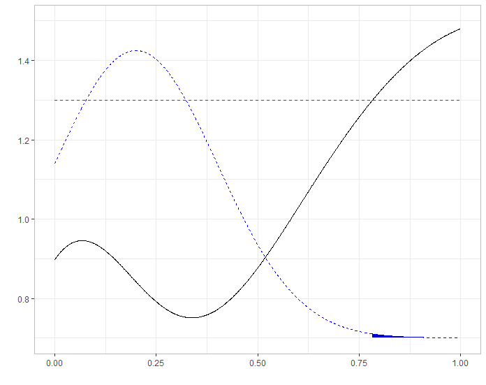

To illustrate our algorithm, we consider a toy example which is just a variant of the one proposed in Section 5.1 of [3]. For all , we set
which is -Lipschitz with . The law of is the restriction of a Gaussian distribution to , i.e.,
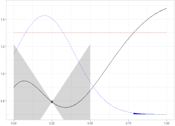
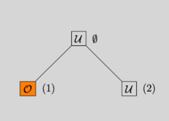
Finally, we take , so that a standard numerical integration gives . This is illustrated on Figure 3, together with the first step of the algorithm. Recall that the evaluation of at point is useless. Indeed, since , the interval is necessarily classified as uncertain (i.e., ). Therefore, the first step consists in computing and , which correspond respectively to vertices and of the tree. From this figure, it is easy to see that is classified as out (i.e., ) while is classified as uncertain (i.e., ). Therefore, there is no need to further investigate the interval .
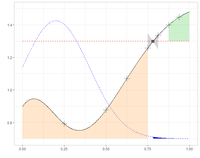
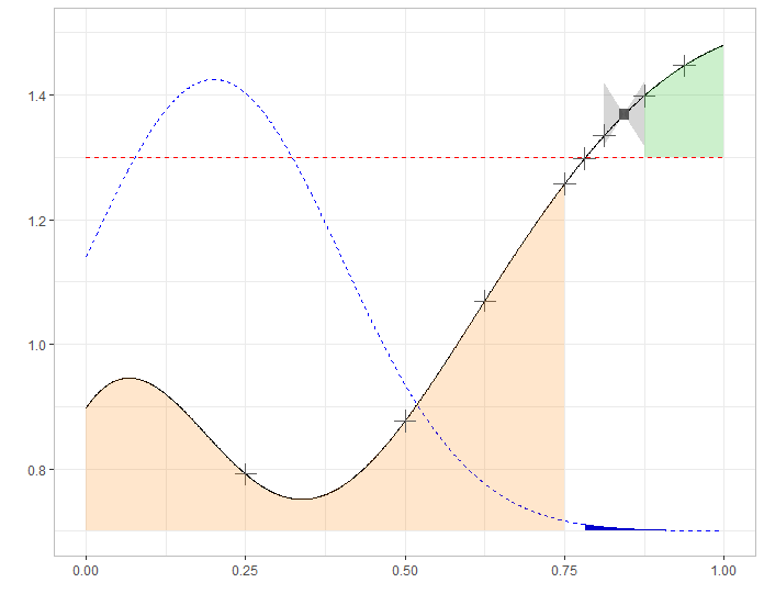
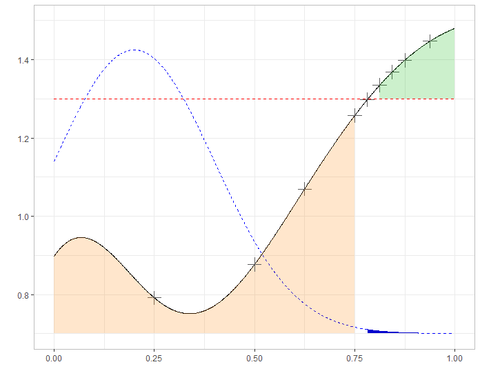
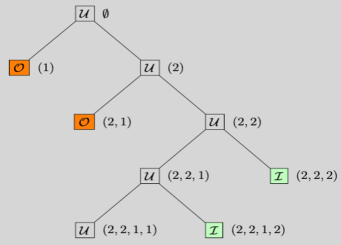
Figure 4 represents step 4 of the algorithm, which consists in evaluating at points (i.e., vertex ) and (i.e., vertex ). These evaluations lead to classify the interval as uncertain (i.e., ) and the interval as included in the failure domain (i.e., ). At this point, the deterministic lower and upper bounds for are thus
and
and the approximation error is simply
Unsurprisingly, one may notice that the upper bound given by Lemma 3.2 is very pessimistic. Indeed, since we know that (see Section 2) and this upper bound can be minorized as follows:
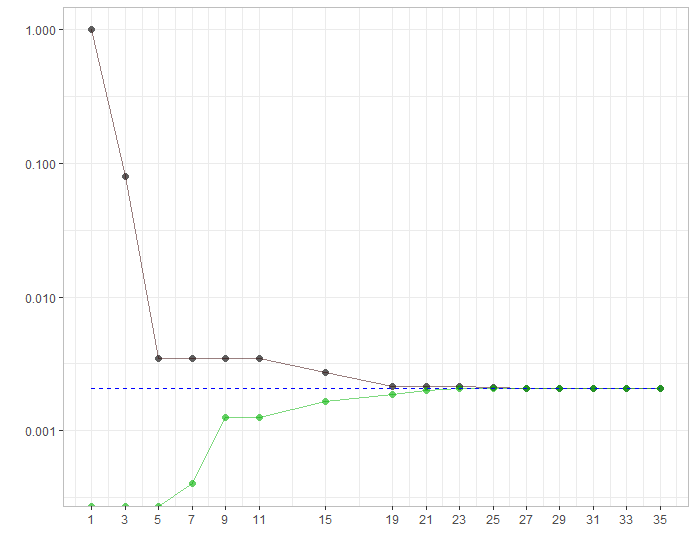
On this toy example, since the law of is simply the restriction of a Gaussian distribution, it is easy to have a very precise numerical approximation of for any dyadic interval and, in turn, for the lower and upper bounds at each step of the algorithm. In other words, we can easily compute the (deterministic) approximation error. The evolution of these bounds and as the number of evaluation points grows is given in Figure 5 for a total budget of calls to .
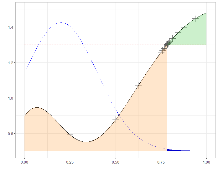
However, in practice, this is usually not possible, hence the use of MCMC techniques as explained in Section 4.2. On our example, up to a normalizing constant, the pdf is defined by
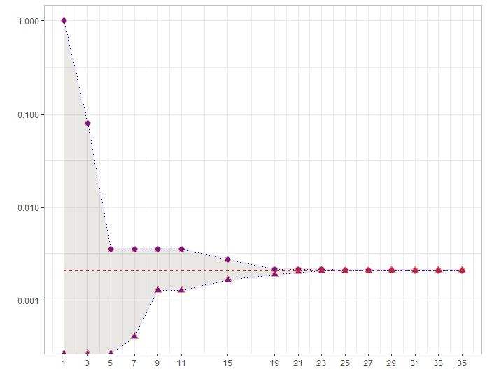
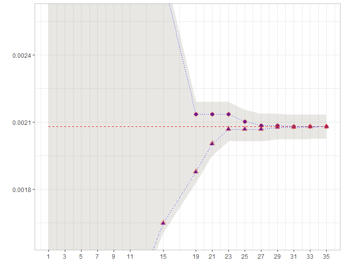
Thus, for any couple of points , the Metropolis ratio that appears in (4.3) is very easy to compute. We have applied this idea for a sample size with Markov transitions for each probability estimation. In this respect, Figure 6 shows that when is much larger than the approximation error, then the latter is much larger than the estimation error. In order to illustrate Remark 4.6, the asymptotic confidence intervals are also given.
6 Optimality
We have established in Theorem 2.2 that after evaluations of the function , the approximation error of our algorithm is of polynomial order when , and of exponential order when . The aim of this section is to show that these bounds are optimal, meaning that they cannot be improved by any other algorithm under the sole general assumptions that we have made on the function .
6.1 The case
When , we consider the following particular case:
-
•
The random variable is uniformly distributed on ;
-
•
The function is defined by for ;
-
•
The threshold is equal to .
Thus, in this setting, the failure probability is equal to . Clearly the function satisfies the Lipschitz Assumption 2 with and the level set Assumption 3 with .
Let us fix an integer for some and arbitrary points in . In the sequel, we construct a function on such that
-
•
for ;
-
•
;
-
•
satisfies Assumptions 2 and 3 with and independent of .
The first fact ensures that any algorithm based on the points leads to the same estimation for and . The second one ensures that is (at least) of order .
First, let us define the face
Consider the set
of dyadic cubes with side length which intersect and the set
of dyadic cubes that intersect and do not contain any point . Since the cardinal of is equal to , the cardinal of is at least .
Second, for any cube and any , let us introduce the piecewise affine function
where . The function is thus supported on and it is -Lipschitz for the norm.
Finally, consider the function defined as follows on :
By construction, the functions and coincide on the cubes that do not belong to . In particular, for any .
Additionally, since is -Lipschitz, the function is -Lipschitz, and therefore Assumption 2 holds with .
For any , if is the center of one has
Therefore for any such that . As a consequence, since has a uniform distribution on , the failure probability associated to satisfies
where .
Finally, let us prove the validity of the level set Assumption 3 for the function . Just like , the absolute value of is smaller than on the cubes and larger elsewhere. Therefore, when , it is readily seen that
For the values , we know that is contained in the union of the cubes . If , then
The cubes are treated by noticing that on such a cube, the function is a rescaled version of the function defined on . The gradient of this function is piecewise constant with and therefore almost everywhere on . In addition vanishes on a polyhedral shaped set of -dimensional measure since in particular if . Using the coarea formula (2.2), this yields
for small enough, and therefore
for all value of up to possibly taking a constant larger than . By rescaling
for all . Summing on all , since and , we find that
This shows that Assumption 3 holds with independent of .
This proves the optimality of the approximation error rate of our algorithm.
6.2 The case
The idea is the same as for the case . More precisely, we consider the following setting:
-
•
The random variable is uniformly distributed on ;
-
•
The function is defined by ;
-
•
The threshold is equal to .
As in the previous subsection, the failure probability is thus equal to , and the function satisfies Assumption 2 with and Assumption 3 with .
Let us fix an integer and points in . As before, the idea is to construct a function on such that
-
•
for ;
-
•
.
-
•
satisfies Assumptions 2 and 3 with and independent of .
First, we define and, for , . To mimic the previous notation, this set of intervals is denoted and, accordingly,
stands for the set of intervals that do not contain any point . Since the cardinal of is equal to , the cardinal of is at least equal to .
Second, for any interval and any , we consider the -Lipschitz function
Finally, we pick one interval and define the function defined as follows
As before, the functions and coincide on . In particular, for any .
Additionally, the function is -Lipschitz, and therefore Assumption 2 holds with . Since vanishes at and (at most) at two other points inside where its gradient is larger than , it is also easily seen that Assumption 3 holds with .
If denotes the center of , then one has
in the case , , and
in the case . Since has Lipschitz constant , it follows that always contains an interval of length larger than . As a consequence, since has a uniform distribution on , the failure probability associated to is such that
with .
This proves the optimality of the approximation error rate of our algorithm.
7 Proof of Theorem 4.4
Consistency and unbiasedness are clear by Remark 4.2. The asymptotic normality is a consequence of the delta method. Remember that for and , we denote
First of all, let us recall the (classical) multidimensional CLT.
Lemma 7.1 (Multidimensional CLT).
For all ,
Let us denote by the random vector and the vector . We have
where the covariance matrix is given by
From the latter we immediately deduce that
Next, we may rewrite as a function of as follows:
The partial derivative of with respect to , denoted , is given by
If is seen a row vector, the delta method ensures that
where
Let us define
We have, since ,
Similarly, we get
Since , this finally yields the claimed expression for .
References
- [1] S.K. Au and J.L. Beck. Estimation of small failure probabilities in high dimensions by subset simulation. Probabilistic Engineering Mechanics, 16(4):263–277, 2001.
- [2] S.K. Au and J.L. Beck. Subset simulation and its application to seismic risk based on dynamic analysis. Journal of Engineering Mechanics, 129(8):901–917, 2003.
- [3] J. Bect, D. Ginsbourger, L. Li, V. Picheny, and E. Vazquez. Sequential design of computer experiments for the estimation of a probability of failure. Stat. Comput., 22(3):773–793, 2012.
- [4] J. Bect, L. Li, and E. Vazquez. Bayesian subset simulation. SIAM/ASA Journal on Uncertainty Quantification, 5(1):762–786, Jan 2017.
- [5] J.A. Bucklew. Introduction to rare event simulation. Springer Series in Statistics. Springer-Verlag, New York, 2004.
- [6] F. Cérou, P. Del Moral, T. Furon, and A. Guyader. Sequential Monte Carlo for rare event estimation. Stat. Comput., 22(3):795–808, 2012.
- [7] F. Cérou and A. Guyader. Fluctuation analysis of adaptive multilevel splitting. Ann. Appl. Probab., 26(6):3319–3380, 2016.
- [8] F. Cérou, A. Guyader, and M. Rousset. Adaptive multilevel splitting: Historical perspective and recent results. Chaos: An Interdisciplinary Journal of Nonlinear Science, 29(4):043108, 2019.
- [9] A. Cohen, R. Devore, G. Petrova, and P. Wojtaszczyk. Finding the minimum of a function. Methods Appl. Anal., 20(4):365–381, 2013.
- [10] O. Ditlevsen and H.O. Madsen. Structural reliability methods, volume 178. Wiley New York, 1996.
- [11] L.C. Evans and R.F. Gariepy. Measure theory and fine properties of functions. Studies in Advanced Mathematics. CRC Press, Boca Raton, FL, 1992.
- [12] A. Guyader, N. Hengartner, and E. Matzner-Løber. Simulation and estimation of extreme quantiles and extreme probabilities. Applied Mathematics and Optimization, 64:171–196, 2011.
- [13] A. Harbitz. An efficient sampling method for probability of failure calculation. Structural Safety, 3(2):109–115, 1986.
- [14] H. Kahn and T.E. Harris. Estimation of particle transmission by random sampling. National Bureau of Standards Appl. Math. Series, 12:27–30, 1951.
- [15] J. Neveu. Arbres et processus de Galton-Watson. Annales de l’I.H.P, 22(2):199–207, 1986.
- [16] C.E. Rasmussen and C.K.I. Williams. Gaussian processes for machine learning. Adaptive Computation and Machine Learning. MIT Press, Cambridge, MA, 2006.
- [17] R. Schöbi, B. Sudret, and J. Wiart. Polynomial-chaos-based Kriging. Int. J. Uncertain. Quantif., 5(2):171–193, 2015.
- [18] L. Tierney. Markov chains for exploring posterior distributions. Ann. Statist., 22(4):1701–1762, 1994. With discussion and a rejoinder by the author.