Structure of the $\Omega$ baryon and the kaon cloud

Abstract

We investigate the effects of the kaon cloud on the electromagnetic and axial-vector form factors of the $\Omega^{-}$ baryon within the framework of the chiral quark-soliton model. We first derive the profile function of the chiral soliton in such a way that the kaon Yukawa tail is properly produced self-consistently. Then, we compute the electromagnetic form factors of the $\Omega^{-}$ baryon. The results for the electromagnetic form factors are compared with the lattice data. We find that the results with the kaon tail employed are in better agreement with the lattice data, compared with those obtained with the pion tail. We also study the axial-vector form factors of the $\Omega^{-}$ baryon, examining the effects of the kaon cloud.

I Introduction

The lowest-lying $\Omega$ baryon is the strangest particle among all hadrons. It is also a member of the baryon decuplet, which was found the latest Barnes:1964pd among the lowest-lying decuplet baryons. The excited state $\Omega(2250)^{-}$ was for the first time found after two decades passed Biagi:1985rn ; Aston:1987bb ; Aston:1988yn . More interestingly, the first excited state $\Omega(2012)^{-}$ was found only very recently Yelton:2018mag ; Jia:2019eav . The Particle Data Group (PDG) summarizes the existence of the four excited states Zyla:2020zbs only. This indicates that the $\Omega$ baryons have been least studied among hyperons. A very recent measurement of the correlation function for the proton ($p$)-$\Omega$ interaction has triggered interest in these $\Omega$ baryons Acharya:2020asf . It reveals that the $p$-$\Omega$ potential is attractive even though the relative distance between $p$ and $\Omega$ goes to zero, which implies a possible existence of the $p$-$\Omega$ bound state Iritani:2018sra . In the meanwhile, the electromagnetic (EM) form factors and axial charges of the ground-state $\Omega$ baryon were computed in lattice quantum chromodynamics (QCD) Alexandrou:2010jv ; Alexandrou:2016xok .

The nucleon has been known to be dressed by the pion cloud in various contexts Yennie:1957 ; Frazer:1959gy ; Frazer:1960zza ; Frazer:1960zzb ; CohenTannoudji:1972gd ; Anselm:1972ir ; Adkins:1983hy ; Frankfurt:1988nt ; Hammer:2006mw ; Meissner:2007tp ; Jenkovszky:2017efs . The pion cloud can be qualitatively understood as the $q\bar{q}$ excitations within the framework of QCD Frankfurt:1988nt or as the pion loop in effective field theory Meissner:2007tp . The large $N_{c}$ (the number of colors) limit of QCD provides yet a lucid point of view on the pion cloud of the nucleon Witten:1979kh . The nucleon emerges as states of the $N_{c}$ valence quarks bound by the pion mean field, which is produced by the presence of the $N_{c}$ valence quarks. This pion mean field can be regarded as the pion cloud. In the Skyrme model with the finite pion mass included, which is the simplest case of the pion mean-field approach, the expectation value of the pion field in a nucleon shows an asymptotic behavior: $\langle\pi^{a}(r)\rangle\sim e^{-m_{\pi}r}x^{i}r^{-2}\langle\sigma_{i}\tau^{a}\rangle$ Adkins:1983hy . A more realistic pion-mean field approach such as the chiral quark-soliton model($\chi$QSM) Diakonov:1987ty ; Diakonov:1997sj provides also the pion cloud from the Dirac-sea polarization or the Dirac-sea continuum Christov:1995vm ; Kim:1995mr .

On the other hand, the $\Omega$ baryon is not coupled to the pion, since it is an isosinglet baryon and consists only of the strange valence quarks. However, the SU(3) baryons are constructed in the $\chi$QSM by embedding the SU(2) soliton into flavor SU(3) space, so all the lowest-lying baryons in the model have the pion tail Witten:1983tw ; Jain:1984gp ; Diakonov:1997sj in common. While this is theoretically consistent, it does not reflect phenomenology properly. Since the hyperons contain the strange quark, the kaon cloud should naturally come into play in describing the structure of them. Even in the case of the nucleon, the kaon cloud provides certain effects when the strangeness in the nucleon is examined Watabe:1995ts ; Kim:1996vj ; Silva:2001st ; Silva:2002ej ; Silva:2005qm . However, in any chiral solitonic approaches, it is impossible to consider both the pion and kaon clouds in a compatible manner. This means that one should choose either the pion cloud or the kaon one, depending on which observables of the hyperons are investigated. For example, the electric form factors of the neutron or neutral hyperons are rather sensitive to the meson tails. Fortunately, the $\Omega$ baryon contains three strange valence quarks and it is not coupled to the pions, so we can choose the kaon tail in place of the pion one. Of course, one may still raise a question about the contributions from the $\eta$ and $\eta^{\prime}$ clouds, since these two pseudoscalar mesons also contain hidden strangeness, so that they can be coupled to the $\Omega$ baryon. The coupling between $\eta$ and $\Omega$ is known to be rather small Yang:2018idi , so the effect of the $\eta$ is expected to be also small on the $\Omega$ baryon. Since the mass of $\eta^{\prime}$ is much larger than the pseudoscalar meson octet, its effect should be suppressed. Thus, as far as we are only concerned with the $\Omega$ baryon, the present approach will still shed light on understanding the effects of kaon cloud or the kaon tail on the structure of the $\Omega$ baryon.

In the present work, we will investigate the EM and axial-vector structures of the $\Omega^{-}$ baryon with the effects of the kaon cloud considered. We first review the kaon properties based on the effective chiral action and fix the relevant parameters such as the pion decay constant, pion and kaon masses. We will then introduce the effective mass of the current strange quark in the Dirac Hamiltonian and solve the classical equation of motion, so that we are able to derive the profile function of the chiral soliton with the proper kaon tail. Then we will perform the symmetry-conserving zero-mode quantization Praszalowicz:1998jm . We will focus on examining the EM and axial-vector form factors of the $\Omega$ baryon, taking into account the $1/N_{c}$ rotational corrections on them. Since the effects of the explicit breaking of flavor SU(3) symmetry are rather small, we do not include them in the present work. Finally, we will compare the present results with those from lattice QCD and explicitly show that the kaon cloud plays an essential role in describing the $\Omega$ baryon.

The present paper is organized as follows: In Section II, we start from the effective chiral action to study the properties of the kaon. Expanding the effective action by using the background field method, one can find the kaon propagator of which the pole yields the mass of the kaon and its residue becomes its decay constant. This process is similar to a usual renormalization of a particle. Then we proceed to the solitonic sector and derive the equation of motion of which the solution leads to the meson mean field. The kaon cloud can be incorporated by using the corresponding quark mass inside the one-body Dirac Hamiltonian. The classical solution, which is identified as the classical mass of the $\Omega$ baryon, possesses the Yukawa tail with the proper kaon mass. This will play a key role in describing the EM and axial-vector form factors of the $\Omega$. In Section III, we briefly recapitulate the formulae for the EM and axial-vector form factors. In Section IV, we present the numerical results and discuss them, comparing them with those from lattice QCD. The last Section is devoted to the summary and conclusion of the present work. In Appendices, we compile the expressions for the EM and axial-vector form factors, derived from the $\chi$QSM.

II Kaon properties and kaon cloud

The effective chiral action and its partition function in Euclidean space are given as

$$Z_{\mathrm{eff}}=\int\mathcal{D}\psi^{\dagger}\mathcal{D}\psi\mathcal{D}\pi^{a}\mathrm{exp}\left[\int d^{4}x\psi^{\dagger}iD(\pi^{a})\psi\right]=\int\mathcal{D}\pi^{a}\mathrm{exp}[-S_{\mathrm{eff}}],$$ (1)

where $S_{\mathrm{eff}}$ represents the effective chiral action expressed by

$$S_{\mathrm{eff}}[\pi]=-N_{c}\mathrm{Tr\;ln}\;(i\not{\partial}+i\hat{m}+iMU^{\gamma_{5}}(\pi^{a})).$$ (2)

Here, $N_{c}$ is the number of colors. $\mathrm{Tr}$ denotes the functional trace over the space-time, spin space, and flavor space. $M$ designates the dynamical quark mass. $\hat{m}$ is the matrix of the current-quark masses

$$\hat{m}=\left(\begin{array}[]{ccc}m_{\mathrm{u}}&0&0\\ 0&m_{\mathrm{d}}&0\\ 0&0&m_{\mathrm{s}}\end{array}\right).$$ (6)

$U^{\gamma_{5}}$ stands for the chiral field expressed by

$$U^{\gamma_{5}}=\frac{1+\gamma_{5}}{2}U+\frac{1-\gamma_{5}}{2}U^{\dagger}$$ (7)

with

$$U(x)=\exp\left[\frac{i}{f}\lambda^{a}\pi^{a}(x)\right].$$ (8)

Here, $f$ is introduced as a scale factor that makes the argument of Eq. (8) dimensionless. $\pi^{a}$ represent the pseudo-Nambu-Goldstone fields expressed as

$$\lambda^{a}\pi^{a}=\left(\begin{array}[]{ccc}\frac{1}{\sqrt{2}}\pi^{0}+\frac{1}{\sqrt{6}}\eta&\pi^{+}&K^{+}\\ \pi^{-}&-\frac{1}{\sqrt{2}}\pi^{0}+\frac{1}{\sqrt{6}}\eta&K^{0}\\ K^{-}&\bar{K}^{0}&-\frac{2}{\sqrt{6}}\eta\end{array}\right).$$ (12)

II.1 Kaon properties

We first examine the meson properties based on the effective chiral action Jaminon:1989wp ; Jaminon:1991vz ; Christov:1995vm . Introducing the meson source $j^{a}$ explicitly, we write the generating functional as follows:

$$\mathcal{Z}[j]=\int\mathcal{D}\pi^{a}e^{-S_{\mathrm{eff}}+j\cdot\pi},$$ (13)

which gives the mesonic two-point correlation function as

$$K^{ab}(x-y)=\left.\frac{\delta^{2}\ln\mathcal{Z}}{\delta j^{a}(x)\delta j^{b}(y)}\right|_{j=0},$$ (14)

where $j\cdot\pi=\int d^{4}xj^{a}(x)\pi^{a}(x)$. Note that in the present model the mesons emerge as low-lying collective $\bar{\psi}\psi$ excitations. Using the background field method Abbott:1981ke , one can decompose the mesonic field $\pi^{a}$ into two parts:

$$\pi^{a}(x)=\pi_{c}^{a}(x)+\delta\pi^{a}(x),$$ (15)

where $\pi^{a}$ is the solution of the classical equation of motion

$$\frac{\delta S}{\delta\pi^{a}(x)}=0,$$ (16)

which is just the same as the classical value of $\pi^{a}$

$$\pi_{c}^{a}(x):=\langle\pi^{a}\rangle=\left.\frac{\delta\ln\mathcal{Z}}{\delta j^{a}(x)}\right|_{j=0}.$$ (17)

Then, the generating functional can be written as

$$\ln\mathcal{Z}=-S_{\mathrm{eff}}[\pi_{c}^{a}]+j\cdot\pi_{c}-\frac{1}{2}\mathrm{Tr}\ln\left[\frac{\delta^{2}S}{\delta\pi\delta\pi}\right]+\frac{1}{2}j\left[\frac{\delta^{2}S}{\delta\pi\delta\pi}\right]^{-1}j,$$ (18)

where the last term is a short-handed notation given as

$$j\left[\frac{\delta^{2}S}{\delta\pi\delta\pi}\right]^{-1}j=\int d^{4}xd^{4}y\,j^{a}(x)\frac{\delta^{2}S}{\delta\pi^{a}(x)\delta\pi^{b}(y)}j^{b}(y).$$ (19)

Note that the first term of Eq. (18) is the effective action that is proportional to $N_{c}$ as shown in Eq. (2). The third term is known to be the one meson-loop contribution, which is proportional to $1/N_{c}$. In the large $N_{c}$ limit, this is suppressed. As shown in Eq. (18), the inverse of the meson propagator is expressed by

$$(K_{\pi}^{ab})^{-1}=\left.\frac{\delta^{2}S_{\mathrm{eff}}}{\delta\pi^{a}(x)\delta\pi^{b}(y)}\right|_{\pi_{c}}.$$ (20)

Expanding $S_{\mathrm{eff}}$ with respect to the meson fields, we obtain the inverse of the pion and kaon propagators in momentum space as follows Blotz:1992pw ; Watabe:1995ts :

$$\frac{1}{Z_{\pi}(p^{2})}\frac{1}{\delta^{4}(0)}\frac{\delta^{2}S_{\mathrm{eff}}}{\delta\pi^{a}(p)\pi^{a}(-p)}\bigg{|}_{p^{2}=-m^{2}_{\pi}} =(p^{2}+m_{\pi}^{2})\bigg{|}_{p^{2}=-m^{2}_{\pi}},\;\;\;a=1,\,2,\,3,$$ (21)

$$\frac{1}{Z_{K}(p^{2})}\frac{1}{\delta^{4}(0)}\frac{\delta^{2}S_{\mathrm{eff}}}{\delta\pi^{a}(p)\pi^{a}(-p)}\bigg{|}_{p^{2}=-m^{2}_{K}} =(p^{2}+m_{K}^{2})\bigg{|}_{p^{2}=-m^{2}_{K}},\;\;\;a=4,\cdots,\,7.$$ (22)

The poles of the meson propagators yield the masses of the pion and kaon

$$m_{\pi}^{2} =\frac{m_{0}I_{1}(M,m_{0})}{Z_{\pi}(p^{2}=-m_{\pi}^{2})}M=(139\,\mathrm{MeV})^{2},$$ (23)

$$m_{K}^{2} =\frac{m_{0}I_{1}(M,m_{0})+m_{\mathrm{s}}I_{1}(M,m_{\mathrm{s}})}{2Z_{K}(p^{2}=-m_{K}^{2})}M+(m_{0}-m_{\mathrm{s}})^{2}=(496\,\mathrm{MeV})^{2},$$ (24)

where

$$I_{1}(M,m_{0})=4N_{c}\int\frac{d^{4}k}{(2\pi)^{4}}\frac{M^{2}}{k^{2}+(M+m_{0})^{2}}.$$ (25)

The $m_{0}$ denotes the average current quark mass i.e., $m_{0}=(m_{u}+m_{d})/2$. $Z_{\pi}$ and $Z_{K}$ stand for the renormalization constants for the pion and kaon wavefunctions, given as

$$Z_{\pi}(p^{2}) =2N_{c}\int\frac{d^{4}k}{(2\pi)^{4}}\frac{M^{2}}{k^{2}+(M+m_{0})^{2}}\frac{M^{2}}{(k+p)^{2}+(M+m_{0})^{2}},$$ (26)

$$Z_{K}(p^{2}) =2N_{c}\int\frac{d^{4}k}{(2\pi)^{4}}\frac{M^{2}}{k^{2}+(M+m_{0})^{2}}\frac{M^{2}}{(k+p)^{2}+(M+m_{s})^{2}}.$$ (27)

Since $I_{1}$ and the renormalization constants are divergent, we use the proper-time regularizations in this work Blotz:1992pw ; Watabe:1995ts .

The meson decay constants $f_{\pi}$ and $f_{K}$ are defined as the transition from the meson state to the vacuum through the axial-vector current

$$\langle 0|A_{\mu}^{a}(x)|\phi^{b}(q)\rangle=iq_{\mu}f_{\phi}e^{-iq\cdot x}\delta^{ab},$$ (28)

where $\phi^{a}$ denotes generically the pion or the kaon. The axial-vector current is given by $A_{\mu}^{a}(x)=i\psi^{\dagger}(x)\gamma_{\mu}\gamma_{5}\frac{\lambda^{a}}{2}\psi(x)$ in Euclidean space. After some length calculations Christov:1995vm ; Blotz:1992pw ; Watabe:1995ts , we obtain the pion and kaon decay constants

$$f_{\phi}(p)=\frac{\sqrt{2Z_{\phi}(p)}}{M}.$$ (29)

Using Eqs. (24) and (29), we obtain the Gell-Mann-Oakes-Renner relation

$$f_{\pi}^{2}m_{\pi}^{2}=-m_{0}i\langle\psi^{\dagger}(0)\psi(0)\rangle_{0},$$ (30)

where the quark condensate $i\langle\psi^{\dagger}(0)\psi(0)\rangle_{0}$ is given by

$$\langle i\psi^{\dagger}(0)\psi(0)\rangle_{0}=-2\frac{I_{1}(M,m_{0})}{M}.$$ (31)

The cut-off parameter $\Lambda$ and the average current quark mass $m_{0}$ are fixed by the pion decay constant and the pion mass, respectively. The dynamical quark mass $M$ is considered to be a free parameter. We take its value to be $M=420$ MeV, with which baryonic properties have been well reproduced Christov:1995vm . The strange current quark mass $m_{\mathrm{s}}=150$ MeV yields the kaon mass $m_{K}=496$ MeV. In the present work, we do not consider the effects of explicit flavor SU(3) symmetry breaking, since their effects are marginal.

II.2 Kaon cloud

Once the parameters of the model were fixed in the mesonic sector, we can proceed to the baryonic sector. The effective chiral action $S_{\mathrm{eff}}$ in Eq. (2) can be expressed in terms of the one-body Dirac Hamiltonian

$$H=\gamma_{4}\gamma_{k}\partial_{k}+M\gamma_{4}U^{\gamma_{5}}+m_{0}\gamma_{4},$$ (32)

of which the eigenenergies and eigenstates of a quark are given by $H|n\rangle=E_{n}|n\rangle$. Having computed the nucleon correlation function (see Refs. Diakonov:1997sj ; Christov:1995vm for details), we obtain the classical mass as

$$M_{\mathrm{cl}}=N_{c}E_{\mathrm{val}}[\pi^{a}]+E_{\mathrm{sea}}[\pi^{a}],$$ (33)

where $E_{\mathrm{val}}$ denotes the energy given by the $N_{c}$ valence quarks filled in the lowest upper Dirac level, which yields the state with baryon number one. $E_{\mathrm{sea}}$ stands for the energy that is required for the pion mean field to be created. This is just the sum of the energies of the quarks filled in the lower Dirac continuum. Note that both the energies $E_{\mathrm{val}}$ and $E_{\mathrm{sea}}$ are given as the functionals of the pion field. Using the classical equation of motion for the pion mean field, we can minimize the energy of the classical nucleon or the chiral soliton. The final solution of the pion mean field is expressed as

$$\pi_{c}^{a}(\bm{x})=n^{a}P(r),$$ (34)

where $P(r)$ designates the profile function of the chiral soliton and $n^{a}$ is a normal vector in isospin space, defined as $n^{a}=x^{a}/\|\bm{x}\|$. In SU(3), we embed this stationary solution into SU(3) as follows:

$$U(\bm{x}):=\begin{pmatrix}\exp[i\bm{n}\cdot\bm{\tau}P(r)]&0\\ 0&1\end{pmatrix}.$$ (35)

$m_{0}$ in Eq. (32) plays an essential role in producing the correct proper Yukawa-type asymptotic behavior of the profile function

$$P(r)=\alpha\exp(-\overline{m}_{\pi}r)\frac{1+\overline{m}_{\pi}r}{r^{2}},$$ (36)

where $\alpha$ denotes a constant that governs the strength of the profile function and $\overline{m}_{\pi}$ represents the generic meson mass that produces a required meson tail. For instance, the $\overline{m}_{\pi}=m_{\pi}=139$ MeV corresponds to the pion cloud whereas $\overline{m}_{\pi}=m_{K}=496$ MeV produces the proper kaon cloud. As mentioned in the Introduction, however, the $\Omega$ is not coupled to the pion but to the kaon. Unfortunately, any chiral solitonic approach cannot take the pion and kaon mean fields into account separately. Since we quantize the SU(3) soliton in Eq. (35) by rotating it slowly in the coordinate and flavor spaces, both the pion and kaon fields have the same pion tail. To investigate properties of the $\Omega^{-}$ baryon, it is natural to consider only the kaon mean field. Of course, this is a rather phenomenological approach but is a necessary one to describe $\Omega^{-}$ more physically. Thus, we increase the value of $m_{0}$ such that the proper kaon cloud is produced, i.e., $\overline{m}_{\pi}=m_{K}=496$ MeV in Eq. (36). Once we obtain the profile function with the kaon cloud, we can compute various properties of $\Omega^{-}$. As will be shown soon, the chiral soliton with the kaon cloud describes the EM and axial-vector form factors far better than that with the pion cloud, when the results are compared with those from lattice QCD. Since we are mainly interested in the effects of the kaon cloud, we will compute all the observables, imposing flavor SU(3) symmetry without its explicit breaking considered.

One may argue that the effects of flavor SU(3) symmetry breaking are too large to be ignored as shown in the Skyrme model with the bound-state approach Callan:1987xt and Yabu-Ando’s approach Yabu:1987hm . In fact, the Yabu-Ando’s approach has been examined within the present framework Blotz:1992pw , where they have computed the mass spectrum of the hyperons. The results showed clearly that the higher-order corrections ($\mathcal{O}(m_{s}^{3})$) are negligible, since they are rather similar to those obtained by the perturbative approach. This indicates that the effects of flavor SU(3) symmetry breaking are rather small. In fact, we found that these effects turned out to be at most 10 % for almost all baryonic observables Christov:1995vm . So, we will only consider the flavor SU(3) symmetric case.

III Electromagnetic and axial-vector form factors of the $\Omega^{-}$ baryon

We first compute the EM form factors of the $\Omega^{-}$ baryon. Since the general formalism was presented in Ref. Kim:2019gka in detail, we briefly recapitulate it. The matrix element of the EM current in Euclidean space is defined as

$$J^{\mu}(x):=i\psi^{\dagger}(x)\gamma^{\mu}\hat{\mathcal{Q}}\psi(x),$$ (37)

where $\psi(x)$ denotes the quark field. The charge operator of the quarks $\hat{\mathcal{Q}}$ is written in terms of the flavor SU(3) Gell-Mann matrices $\lambda_{3}$ and $\lambda_{8}$

$$\hat{\mathcal{Q}}=\begin{pmatrix}\frac{2}{3}&0&0\\ 0&-\frac{1}{3}&0\\ 0&0&-\frac{1}{3}\end{pmatrix}=\frac{1}{2}\left(\lambda_{3}+\frac{1}{\sqrt{3}}\lambda_{8}\right).$$ (38)

The matrix elements of the EM current between the $\Omega^{-}$ baryons can be parametrized by four form factors $F_{i}$ ($i=1,\cdots,4$) as follows:

$$\langle\Omega^{-}(p^{\prime},s)|J^{\mu}(0)|\Omega^{-}(p,s)\rangle =-\overline{u}^{\alpha}(p^{\prime},s)\left[\gamma^{\mu}\left\{F_{1}(q^{2})\eta_{\alpha\beta}+F_{3}(q^{2})\frac{q_{\alpha}q_{\beta}}{4M_{\Omega}^{2}}\right\}\right.$$ (39)

$$\hskip 56.9055pt\left.+\,i\frac{\sigma^{\mu\nu}q_{\nu}}{2M_{\Omega}}\left\{F_{2}(q^{2})\eta_{\alpha\beta}+F_{4}(q^{2})\frac{q_{\alpha}q_{\beta}}{4M_{\Omega}^{2}}\right\}\right]{u}^{\beta}(p,s),$$ (40)

where $M_{\Omega}$ stands for the mass of the $\Omega^{-}$ baryon in the decuplet. $q_{\alpha}$ represents the momentum transfer $q_{\alpha}=p_{\alpha}^{\prime}-p_{\alpha}$ and its square is given by $q^{2}=-Q^{2}$ with $Q^{2}>0$. $u^{\alpha}(p,\,s)$ designates the Rarita-Schwinger spinor, carrying the momentum $p$ and the spin component $s$ projected along the direction of the momentum.

The multipole EM form factors can be expressed in terms of $F_{i}$ in Eq. (40)

$$G_{E0}(Q^{2})=\left(1+\frac{2}{3}\tau\right)[F_{1}-\tau F_{2}]-\frac{1}{3}\tau(1+\tau)[F_{3}-\tau F_{4}],$$ (41)

$$G_{E2}(Q^{2})=[F_{1}-\tau F_{2}]-\frac{1}{2}(1+\tau)[F_{3}-\tau F_{4}],$$ (42)

$$G_{M1}(Q^{2})=\left(1+\frac{4}{5}\tau\right)[F_{1}+F_{2}]-\frac{2}{5}\tau(1+\tau)[F_{3}+F_{4}],$$ (43)

$$G_{M3}(Q^{2})=[F_{1}+F_{2}]-\frac{1}{2}(1+\tau)[F_{3}+F_{4}],$$ (44)

where $\tau=Q^{2}/4M_{\Omega}^{2}$. These four form factors are called, respectively, the electric or Coulomb monopole (E0), magnetic dipole (M1), electric quadrupole (E2), and magnetic octupole (M3) form factors. At $Q^{2}=0$, the values of these form factors are reduced to the charge, the magnetic dipole moment, the electric quadrupole moment, and the magnetic octupole moment, respectively

$$e_{\Omega} =eG_{E0}(0),$$ (45)

$$\mu_{\Omega} =G_{M1}(0)\left(\frac{M_{N}}{M_{\Omega}}\right)\mu_{N},$$ (46)

$$Q_{\Omega} =\frac{e}{M_{\Omega}^{2}}G_{E2}(0),$$ (47)

$$O_{\Omega} =\frac{e}{M_{\Omega}^{3}}G_{M3}(0).$$ (48)

Note that the electric quadrupole moment is proportional to $1/N_{c}$ and the magnetic octupole moment is of order $1/N_{c}^{2}$. Thus, M3 vanishes when we consider the corrections to order $1/N_{c}$.

In the Breit frame, i.e., $\bm{p^{\prime}}=-\bm{p}=\bm{q}/2$, the electric and magnetic parts of the multipole form factors are related to the temporal and spatial components of the EM current, respectively

$$G_{E0}(Q^{2}) =\int\frac{d\Omega_{q}}{4\pi}\langle\Omega^{-}(p^{\prime},3/2)|J^{0}(0)|\Omega^{-}(p,3/2)\rangle,$$ (49)

$$G_{E2}(Q^{2}) =-\int d\Omega_{q}\sqrt{\frac{5}{4\pi}}\frac{3}{2}\frac{1}{\tau}\langle\Omega^{-}(p^{\prime},3/2)|Y^{*}_{20}(\Omega_{q})J^{0}(0)|\Omega^{-}(p,3/2)\rangle,$$ (50)

$$G_{M1}(Q^{2}) =\frac{3M_{\Omega}}{4\pi}\int\frac{d\Omega_{q}}{iQ^{2}}q^{i}\epsilon^{ik3}\langle\Omega^{-}(p^{\prime},3/2)|J^{k}(0)|\Omega^{-}(p,3/2)\rangle,$$ (51)

$$G_{M3}(Q^{2}) =-\frac{35M_{\Omega}}{8}\sqrt{\frac{5}{\pi}}\int\frac{d\Omega_{q}}{iQ^{2}\tau}q^{i}\epsilon^{ik3}\langle\Omega^{-}(p^{\prime},3/2)|\left(Y^{*}_{20}(\Omega_{q})+\sqrt{\frac{1}{5}}Y^{*}_{00}(\Omega_{q})\right)J^{k}(0)|\Omega^{-}(p,3/2)\rangle.$$ (52)

The matrix elements of the EM current can be computed within the framework of the $\chi$QSM, which was already done in Ref. Kim:2019gka , with the rotational $1/N_{c}$ and linear $m_{\mathrm{s}}$ corrections considered. For detailed calculations, we refer to Ref. Kim:2019gka . For convenience, we compile the expressions for the EM form factors of the $\Omega$ baryon in Appendix A.

We can derive the axial-vector form factors of the $\Omega^{-}$ baryon in a similar manner. Since $\Omega^{-}$ is an isosinglet baryon, the triplet components of the $\Omega^{-}$ axial-vector form factors vanish. The axial-vector current of the quark field is defined as

$$A_{\mu}^{0}:=i\psi^{\dagger}(x)\gamma_{\mu}\gamma^{5}\psi(x),\;\;\;A_{\mu}^{8}(x):=i\psi^{\dagger}(x)\gamma_{\mu}\gamma^{5}\frac{\lambda^{8}}{2}\psi(x).$$ (53)

The matrix elements of the axial-vector currents for the $\Omega^{-}$ baryon can again be parametrized by four different real form factors as follows:

$$\langle\Omega^{-}(p^{\prime},s)|A_{\mu}^{0}(0)|\Omega^{-}(p,s)\rangle =-\overline{u}^{\alpha}(p^{\prime},s)\left[\gamma_{\mu}\left\{g_{1}^{(0)}(q^{2})\eta_{\alpha\beta}+h_{1}^{(0)}(q^{2})\frac{q_{\alpha}q_{\beta}}{4M_{\Omega}^{2}}\right\}\right.$$ (54)

$$\hskip 56.9055pt\left.+\,\frac{q^{\mu}}{2M_{\Omega}}\left\{g_{3}^{(0)}(q^{2})\eta_{\alpha\beta}+h_{3}^{(0)}(q^{2})\frac{q_{\alpha}q_{\beta}}{4M_{\Omega}^{2}}\right\}\right]\gamma^{5}u^{\beta}(p,s),$$ (55)

$$\langle\Omega^{-}(p^{\prime},s)|A_{\mu}^{8}(0)|\Omega^{-}(p,s)\rangle =-\overline{u}^{\alpha}(p^{\prime},s)\left[\gamma_{\mu}\left\{g_{1}^{(8)}(q^{2})\eta_{\alpha\beta}+h_{1}^{(8)}(q^{2})\frac{q_{\alpha}q_{\beta}}{4M_{\Omega}^{2}}\right\}\right.$$ (56)

$$\hskip 56.9055pt\left.+\,\frac{q^{\mu}}{2M_{\Omega}}\left\{g_{3}^{(8)}(q^{2})\eta_{\alpha\beta}+h_{3}^{(8)}(q^{2})\frac{q_{\alpha}q_{\beta}}{4M_{\Omega}^{2}}\right\}\right]\frac{\gamma^{5}}{2}{u}^{\beta}(p,s).$$ (57)

Since the axial-vector form factors $g_{1}^{(0,\,8)}$ and $g_{3}^{(0,\,8)}$ are the most important ones among the axial-vector form factors, we will concentrate on them in the present work. Moreover, they are directly related to the strong coupling constants for the $\eta\Omega\Omega$ and $\eta^{\prime}\Omega\Omega$ vertices Yang:2018idi . In the Breit frame, the form factors defined in Eq  (57) are expressed in terms of the spatial parts of the axial-vector current projected by the spherical basis vectors $\bm{e}_{n}$

$$g^{(0,\,8)}_{1}(Q^{2}) =-\sqrt{\frac{3}{2}}\frac{M_{\Omega}}{E_{\Omega}}\langle\Omega^{-}(p^{\prime},3/2)|\bm{e}_{1}\cdot\left(\bm{A}^{0}(0),2\bm{A}^{8}(0)\right)|\Omega^{-}(p,1/2)\rangle,$$ (58)

$$g^{(0,\,8)}_{3}(Q^{2}) =-\frac{4M^{2}_{\Omega}}{Q^{2}}\left[\langle\Omega^{-}(p^{\prime},3/2)|\bm{e}_{0}\cdot\left(\bm{A}^{0}(0),2\bm{A}^{8}(0)\right)|\Omega^{-}(p,3/2)\rangle\right.$$ (59)

$$\left.\hskip 56.9055pt-\,\sqrt{\frac{3}{2}}\frac{M_{\Omega}}{E_{\Omega}}\langle\Omega^{-}(p^{\prime},3/2)|\bm{e}_{1}\cdot\left(\bm{A}^{0}(0),2\bm{A}^{8}(0)\right)|\Omega^{-}(p,1/2)\rangle\right],$$ (60)

where $E_{\Omega}$ corresponds to the energy of the corresponding baryon, i.e. $E_{\Omega}=\sqrt{M^{2}_{\Omega}+Q^{2}/4}$, and the spherical unit vectors $\bm{e}_{n}$ are expressed in terms of the Cartesian basis vectors $\bm{e}_{0}=\hat{\bm{z}}$, $\bm{e}_{1}=-(\hat{\bm{x}}+i\hat{\bm{y}})/\sqrt{2}$, $\bm{e}_{-1}=(\hat{\bm{x}}-i\hat{\bm{y}})/\sqrt{2}$. The matrix elements of the projected currents $\bm{e}_{i}\cdot\left(\bm{A}^{0}(0),2\bm{A}^{8}(0)\right)$ can be computed within the framework of the $\chi$QSM. The detail formalism can be found in Ref. Jun:2020lfx . We list the expressions for the EM form factors of the $\Omega$ baryon in Appendix B.

IV Results and discussion

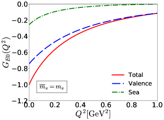
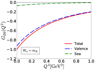
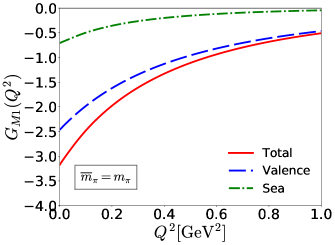
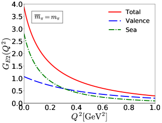
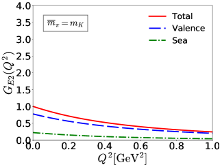
Figure 1: Numerical results for the E0, M1, E2 form factors of the $\Omega^{-}$ baryon with both the pion and kaon clouds considered. In the left panels those with the pion cloud are drawn whereas in the right panels those with the kaon cloud are depicted. The dashed and dot-dashed curves exhibit the valence-quark (level-quark) and sea-quark (Dirac continuum) contributions, respectively. The solid curves show the total contributions.

We first present the results for the E0, M1, and E2 form factors of the $\Omega^{-}$ baryon, drawing separately the valence- and sea-quark contributions. We already expect that the sea-quark contributions will be greatly changed by replacing the pion cloud with the kaon one. In the upper-left (right) panel of Fig. 1, we depict the numerical results for the E0 form factors with the pion (kaon) cloud employed. Since the E0 form factor of $\Omega^{-}$ at $Q^{2}=0$ should be the same as its charge as shown in Eq. (48) because of the U(1) gauge symmetry, one can see that replacing the pion cloud with the kaon one enhances the valence-quark contribution but suppresses that of the sea-quark. We find similar features for the M1 and E2 form factors by observing the results presented respectively in the middle and lower panels of Fig. 1. In particular, the sea-quark contribution to the E2 form factor is drastically reduced when the pion cloud is replaced with the kaon cloud. As already discussed in Ref. Kim:2019gka , the E2 form factors of the baryon decuplet are in general very sensitive to the tail. This indicates that the deformation of a baryon with spin 3/2 is governed by the sea-quark contribution or the meson clouds. On the other hand, the valence-quark contributions are not much influenced by changing the meson clouds.

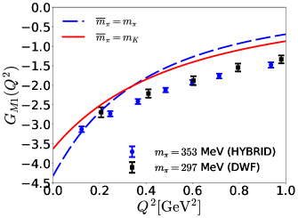
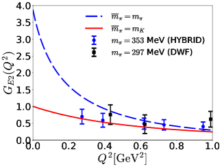
Figure 2: Comparison of the present results for the EM form factors of the $\Omega^{-}$ baryon with those from lattice data. The solid curves draw the results with the kaon cloud whereas the dashed ones depict those with the pion cloud. The lattice data are taken from Ref. Alexandrou:2010jv . The magnetic form factor is given in units of the soliton magneton, of which the reason is explained in the text.

In Fig. 2, we compare the present results for the EM form factors of $\Omega^{-}$ with those from lattice QCD Alexandrou:2010jv . In the upper left panel of Fig. 2, we draw the numerical results for the E0 form factor of the $\Omega^{-}$. The result with the kaon cloud falls off more slowly than that with the pion cloud and is in better agreement with the lattice data, compared with that with the pion cloud. It is well known that the lattice data on the EM form factors of the nucleon Capitani:2015sba ; Hansen:2016fzj with the unphysical pion mass fall off more slowly than the experimental data as $Q^{2}$ increases. Even the physical pion mass is used, the lattice results for the EM form factors of the nucleon still overestimate the experimental data Alexandrou:2017ypw . Thus, it is natural to observe that the present results for the E0 form factor of the $\Omega^{-}$ baryon fall off faster than the lattice data, as shown in the upper left panel of Fig. 2. However, the result with the kaon cloud is markedly closer to the lattice data than those with the pion one.

In the upper right panel of Fig. 2, we depict the results for the M1 form factor of $\Omega^{-}$. Before we discuss them, we want to mention that the magnetic dipole moments of the SU(3) baryons are given in terms of the soliton magneton instead of the nuclear magneton. There are two reasons for doing this. Firstly, while the mass differences of the baryon octet and decuplet and even singly heavy baryons are well reproduced within the $\chi$QSM Blotz:1992pw ; Christov:1995vm ; Kim:2018xlc ; Kim:2019rcx , the absolute values of these masses are always overestimated. This is a well-known problem in any chiral solitonic approaches. Secondly, the magnetic dipole moments of the baryon octet and decuplet are always underestimated by about 30 %. Thus, it is theoretically consistent and empirically plausible to express the values of the magnetic dipole moments in units of the soliton magneton, which improves theoretical results for the magnetic dipole moments in comparison with the experimental data. As shown in the upper right panel of Fig. 2, the result for the M1 form factors of $\Omega^{-}$ with the kaon cloud again is in better agreement with the lattice data, compared with that with the pion one.

The lower panel of Fig. 2 illustrates how the kaon cloud suppresses the E2 form factor of $\Omega^{-}$. It is remarkable that the kaon cloud reduces the magnitude of the E2 form factor almost by factor 4 and the numerical result with the kaon cloud is in far better agreement with the lattice data, compared to that with the pion cloud. As already seen in Ref. Kim:2019gka , the sea-quark contribution or the meson-cloud effect is dominant over that of the valence quarks. This is natural, since the E2 form factor measures how much the baryon with spin 3/2 is deformed from the spherical shape. This implies that the $\Omega^{-}$ baryon is less deformed than the $\Delta$ isobar, since it is energetically easier to create the pion cloud than the kaon one. Comparing the results with the lattice data, we observe that the numerical result with the kaon cloud is indeed in good agreement with them. On the other hand, that with the pion cloud deviates from the lattice data in smaller $Q^{2}$ regions.

Table 1: Numerical results for the electromagnetic observables in comparison with the lattice data Alexandrou:2016xok . Those for the magnetic dipole moment of the $\Omega^{-}$ baryon are compared with the experimental data Zyla:2020zbs .

	$\langle r^{2}\rangle_{E}$ (fm2)	$\mu$ ($\mu_{N}$)	$G_{E2}(0)$
$\bar{m}_{\pi}=m_{\pi}$	$0.83$	$-2.48$	$3.88$
$\bar{m}_{\pi}=m_{K}$	$0.51$	$-2.04$	$1.00$
Exp Zyla:2020zbs	$-$	$-2.02(5)$	$-$
LQCD Alexandrou:2010jv	$0.348(52)$	$-1.875(399)$	$0.898(60)$

Table 2: Magnetic dipole moment of the $\Omega^{-}$ baryon in comparison with the results from lattice QCD Leinweber:1992hy ; Aubin:2008qp ; Boinepalli:2009sq , the relativistic quark model Schlumpf:1993rm , next-to-leading-order HB$\chi$PT Butler:1993ej , large $N_{c}$ Luty:1994ub , QCD sum rules Lee:1997jk , the chiral quark model Wagner:2000ii , covariant $\chi$PT Geng:2009ys , $\chi$PT Li:2016ezv and the experimental data Zyla:2020zbs .

	$\overline{m}_{\pi}=m_{\pi}$	$\overline{m}_{\pi}=m_{K}$	Zyla:2020zbs	Leinweber:1992hy	Boinepalli:2009sq	Aubin:2008qp	Butler:1993ej	Geng:2009ys	Li:2016ezv	Luty:1994ub	Schlumpf:1993rm	Wagner:2000ii	Lee:1997jk
$\mu_{\Omega^{-}}(\mu_{N})$	$-2.48$	$-2.04$	$-2.02(5)$	$-1.73(22)$	$-1.70(7)$	$-1.93(8)$	$-1.94(22)$	$-2.02$	$-2.02(5)$	$-1.94$	$-2.35$	$-2.13$	$-1.49(45)$

Table 3: Electric quadrupole moment of the $\Omega^{-}$ baryon in comparison with the quark model Krivoruchenko:1991pm , HB$\chi$PT Butler:1993ej , the Skyrme model Oh:1995hn , large $N_{c}$ Buchmann:2002et , the chiral quark model Wagner:2000ii , the QCD sum rules Azizi:2008tx ; Aliev:2009pd .

	$\overline{m}_{\pi}=m_{\pi}$	$\overline{m}_{\pi}=m_{K}$	Butler:1993ej	Buchmann:2002et	Krivoruchenko:1991pm	Oh:1995hn	Wagner:2000ii	Azizi:2008tx ; Aliev:2009pd
$Q_{\Omega^{-}}(\mathrm{fm}^{2})$	$0.054$	$0.014$	$0.009(5)$	$0.027$	$0.028$	$0$	$0.026$	$0.12(4)$

Table 1 lists the numerical results for the charge radius, magnetic dipole moment, and the value of the E2 form factor at $Q^{2}=0$ i.e., $G_{E2}(0)$ of the $\Omega^{-}$ baryon. Those with the kaon cloud are prominently in better agreement with the lattice data than those with the pion cloud. In the case of the magnetic dipole moment, we also find that the result with the kaon cloud is in better agreement with the result from lattice QCD. In Tables 2 and 3, we compare the present results respectively for the magnetic dipole moment and the electric quadrupole moment of the $\Omega^{-}$ baryon with those obtained from other approaches. As already discussed in Ref. Kim:2019gka , the present numerical result for the E2 moment turns out to be larger than those from other works. We now can see that this discrepancy arises from the fact that only when the kaon cloud is properly considered, the E2 moment can be correctly reproduced. This emphasizes the important role of the kaon cloud in describing the $\Omega^{-}$ baryon.

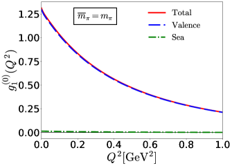
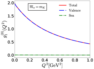
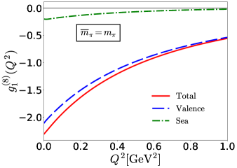
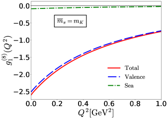
Figure 3: Numerical results for the $g_{1}^{(0)}$ and $g_{1}^{(8)}$ axial-vector form factors of the $\Omega^{-}$ baryon with both the pion and kaon clouds considered. In the left panels those with the pion cloud are drawn whereas in the right panels those with the kaon cloud are depicted. The dashed and dot-dashed curves exhibit the valence-quark (level-quark) and sea-quark (Dirac continuum) contributions, respectively. The solid curves show the total contributions.

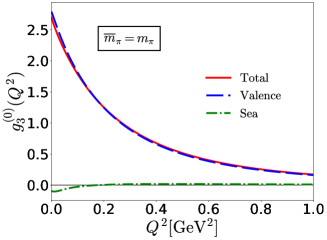
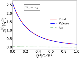
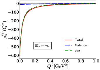
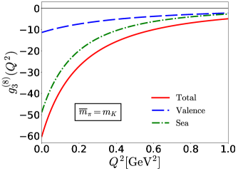
Figure 4: Numerical results for the $g_{3}^{(0)}$ and $g_{3}^{(8)}$ axial-vector form factors of the $\Omega^{-}$ baryon with both the pion and kaon clouds considered. In the left panels those with the pion cloud are drawn whereas in the right panels those with the kaon cloud are depicted. The dashed and dot-dashed curves exhibit the valence-quark (level-quark) and sea-quark (Dirac continuum) contributions, respectively. The solid curves show the total contributions.

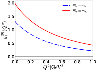
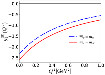
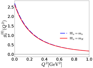
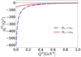
Figure 5: Comparison of the present results for the axial-vector form factors of the $\Omega^{-}$. The solid curves draw the results with the kaon cloud whereas the dashed ones depict those with the pion cloud.

We now turn to the axial-vector form factors of the $\Omega^{-}$ baryon. Since it is an isoscalar baryon, it is not coupled to the isovector axial-vector current. So, we first consider the singlet axial-vector form factors of $\Omega^{-}$. The axial-vector form factor $g_{1}^{(0)}$ is related to the spin content of the $\Omega$ baryon, i.e., its value at $Q^{2}=0$ has the same physical meaning of $g_{A}^{(0)}$ of the nucleon. The value of $g_{A}^{(0)}$ becomes null in the Skryme model Brodsky:1988ip ; Ellis:1988mn , whereas it acquires a small value from the rotational $1/N_{c}$ corrections in the $\chi$QSM Blotz:1993dd ; Blotz:1994wi . The results from the $\chi$QSM were later improved by employing the symmetry-conserving quantization Praszalowicz:1998jm ; Silva:2005fa . In Ref. Silva:2005fa , it was shown that the kaon cloud does not much change the strange component of the singlet axial charge and the values of $g_{A}^{(0)}$, $g_{A}^{(3)}$ and $g_{A}^{(8)}$ for the nucleon were obtained respectively to be $g_{A}^{(0)}=0.367$, $g_{A}^{(3)}=1.176$, and $g_{A}^{(8)}=0.360$. Subtle differences between these two models were discussed very in detail in Ref. Wakamatsu:1996jn . Figure 3 illustrates how the valence- and sea-quark contributions are changed by the replacement of the pion cloud with the kaon one. Interestingly, the sea-quark contributions are not much changed by the kaon cloud. However, once the kaon cloud is considered, the valence-quark contribution makes $g_{1}^{(0)}(Q^{2})$ enhanced by about 40 %. This can be observed clearly in the upper left panel of Fig. 5. On the other hand, the kaon cloud increases the value of $g_{1}^{(8)}$ by about 10 % (see Figs. 3 and 5). It is interesting to compare the present result for $g_{1}^{(0)}(Q^{2})$ of $\Omega^{-}$ with that of the $\Delta^{+}$ isobar. When the pion cloud is adopted, there is almost no difference between $g_{1}^{(0)}(Q^{2})$ of the $\Delta^{+}$ and $\Omega^{-}$ baryons, as presented in Ref. Jun:2020lfx . However, once we replace the pion cloud with the kaon one, the situation is drastically changed. $g_{1}^{(0)}$ of $\Omega^{-}$ is about 40 % larger than that of $\Delta^{+}$. This indicates that the up and down sea quarks are less likely to pop up in the $\Omega^{-}$ baryons, compared with the role of the strange quark in the $\Delta^{+}$ baryon. So, the sea quarks inside $\Omega^{-}$ are less polarized. In the lower panel of Fig. 3, we depict the results for $g_{1}^{(8)}$. The valence-quark contribution is enhanced by about 15 % whereas that of the sea-quark is suppressed by about 50 %, when the kaon cloud was employed. Altogether, the result for $g_{1}^{(8)}$ is enhanced by about 12 % with the kaon cloud used, as shown more clearly in the upper right panel of Fig. 5.

In the upper panel of Fig. 4 we draw the numerical results for $g_{3}^{(0)}$, which show that $g_{3}^{(0)}$ is almost not affected by the replacement of the pion cloud with the kaon one. However, the kaon cloud reduces remarkably the magnitude of $g_{1}^{(8)}$ as shown in the lower panel of Fig. 4 by about factor 10. In particular, the contribution of the valence quarks is not much influenced by the replacement of the pion cloud with the kaon one, whereas the sea-quark contribution is tremendously lessened. This can be understood by the fact that the expression for $g_{3}^{(8)}$ is rather sensitive to the tail part of the soliton profile function. So far, there has been no lattice data on the $g_{3}^{(8)}$ form factor of the $\Omega^{-}$ baryon. It would be very interesting, if one could compare the present result with the lattice data in the near future. In Fig. 5, we compare the results for the axial-vector form factors with the kaon cloud to those with the pion one. Table 4 summarizes the values of the axial charges of the $\Omega^{-}$ baryon, comparing them with the lattice data Alexandrou:2016xok . With the kaon cloud considered, the present results for $g_{1}^{(0)}$ are in better agreement with the lattice data. However, we do not see any particular improvement for $g_{1}^{(8)}$ by replacing the pion cloud with the kaon one.

Table 4: Numerical results for the axial charges $g_{1}^{(0,8)}$ and $g_{3}^{(0,8)}$ in comparison with those from lattice QCD (LQCD) Alexandrou:2016xok . Since the expressions for the octet axial-vector current $A_{\mu}^{8}(x)$ in Ref. Alexandrou:2016xok are different from the present one by $\sqrt{3}$, we have considered it for comparison.

	$g^{(0)}_{1}(0)$	$g^{(8)}_{1}(0)$	$g^{(0)}_{3}(0)$	$g^{(8)}_{3}(0)$
$\overline{m}_{\pi}=m_{\pi}$	$1.313$	$-3.863$	$2.696$	$-605.734$
$\overline{m}_{\pi}=m_{K}$	$1.979$	$-4.296$	$2.619$	$-60.290$
LQCD $(m_{\pi}=213\;\mathrm{MeV})$	$2.0365\pm 0.0303$	$-4.0731\pm 0.0606$	-	-
LQCD $(m_{\pi}=256\;\mathrm{MeV})$	$1.9606\pm 0.0376$	$-3.9212\pm 0.0752$	-	-
LQCD $(m_{\pi}=302\;\mathrm{MeV})$	$2.0215\pm 0.0441$	$-4.0431\pm 0.0883$	-	-
LQCD $(m_{\pi}=373\;\mathrm{MeV})$	$1.9044\pm 0.0439$	$-3.8087\pm 0.0877$	-	-
LQCD $(m_{\pi}=432\;\mathrm{MeV})$	$1.9562\pm 0.0457$	$-3.9125\pm 0.0915$	-	-

V Summary and conclusions

In the present work, we investigated the effects of the kaon cloud on the electromagnetic and axial-vector properties of the $\Omega^{-}$ baryon. We first briefly reviewed the mesonic sector, explaining how the kaonic properties can be described within the present framework. The cutoff parameters and the average value of the up and down quark masses were fixed by the pion decay constant and the pion mass, respectively. Then we were able to reproduce the kaon mass. The average quark mass of the up and down quarks inside the one-body Dirac Hamiltonian produces the asymptotic pion Yukawa tail of the solitonic profile function and this proper behavior of the Yukawa tail is called the pion tail. Since the $\Omega^{-}$ baryon consists of the triple strange valence quarks, the kaon cloud is required. Thus, we changed the value of the average quark mass in such a way that the proper kaon Yukawa tail was produced. While this is theoretically somewhat inconsistent, it improves phenomenologically the description of the $\Omega^{-}$ baryon. As far as we consider only the $\Omega^{-}$ baryon, this kaon tail provides even a more plausible theoretical ground than the pion one. Employing the kaon cloud, we computed the electromagnetic and axial-vector form factors of the $\Omega^{-}$ baryon. In the case of the electromagnetic form factors, the kaon cloud suppresses mainly the sea-quark contributions whereas those of the valence quarks are not much affected. When the kaon cloud is considered, the present results for the E0, M1, and E2 form factors are in better agreement with the lattice data in comparison with those obtained by the pion cloud. The results for the electric quadrupole moment are also in better agreement with those from other works. We then calculated the axial-vector form factors of the $\Omega^{-}$ baryon and discussed the differences between the results with the kaon cloud and those with the pion one. The value of the singlet axial-vector form factor $g_{1}^{(0)}$ is increased by about 40 %, whereas the octet one $g_{1}^{(8)}$ is enhanced by about 12 %. While the $g_{3}^{(0)}$ form factor is almost kept intact, $g_{3}^{(8)}$ was drastically reduced by about factor 10 when the pion cloud is replaced with the kaon one.

Since the strange valence quark is deeply related to the kaon cloud, it is of great importance to examine how the kaon cloud affects all other hyperons with double strange valence quarks. In particular, because the singlet axial charges $g_{1}^{(0)}(0)$ provide information on the spin content of these baryons, one has to consider the effects of the kaon cloud. The corresponding investigation is under way.

Appendix A Electromagnetic form factors

In Appendix A, we compile all the expresstions for the EM form factors of the $\Omega$ baryon within the framework of the $\chi$QSM.

$${G}_{E0}(Q^{2})=e_{\Omega}\int d^{3}rj_{0}(Q|\bm{r}|)\left[\frac{1}{24}{\mathcal{B}}(\bm{r})+\frac{5}{8I_{1}}{\mathcal{I}}_{1}(\bm{r})+\frac{1}{4I_{2}}{\mathcal{I}}_{2}(\bm{r})\right],$$ (61)

where densities of the electric form factor are written explicitly as

$$\frac{1}{N_{c}}{\cal{B}}(\bm{r})= \langle\mathrm{val}|\bm{r}\rangle\langle\bm{r}|\mathrm{val}\rangle-\frac{1}{2}\sum_{n}\mathrm{sign}(E_{n})\langle n|\bm{r}\rangle\langle\bm{r}|n\rangle,$$ (62)

$$\frac{6}{N_{c}}{\cal{I}}_{1}(\bm{r})= \sum_{n\neq\mathrm{val}}\frac{1}{E_{n}-E_{\mathrm{val}}}\langle\mathrm{val}|\bm{r}\rangle\bm{\tau}\langle\bm{r}|n\rangle\cdot\langle n|\bm{\tau}|\mathrm{val}\rangle+\frac{1}{2}\sum_{n,m}\langle n|\bm{\tau}|m\rangle\cdot\langle m|\bm{r}\rangle\bm{\tau}\langle\bm{r}|n\rangle{\mathcal{R}}_{3}(E_{n},E_{m}),$$ (63)

$$\frac{4}{N_{c}}{\cal{I}}_{2}(\bm{r})= \sum_{n^{0}}\frac{1}{E_{n^{0}}-E_{\mathrm{val}}}\langle n^{0}|\mathrm{val}\rangle\langle\mathrm{val}|\bm{r}\rangle\langle\bm{r}|n^{0}\rangle+\sum_{n,m^{0}}\langle n|m^{0}\rangle\langle m^{0}|\bm{r}\rangle\langle\bm{r}|n\rangle{\mathcal{R}}_{3}(E_{n},E_{m^{0}}).$$ (64)

The expression for the magnetic dipole form factor of the $\Omega$ baryon is written as

$${G}_{M1}(Q^{2})=-\frac{1}{8}e_{\Omega}\frac{M_{\Omega}}{Q}\int d^{3}r\frac{j_{1}(Q|\bm{r}|)}{|\bm{r}|}\left[\left({\cal{Q}}_{0}(\bm{r})+\frac{1}{I_{1}}{\cal{Q}}_{1}(\bm{r})\right)+\frac{1}{2}\frac{1}{I_{1}}{\cal{X}}_{1}(\bm{r})+\frac{1}{2}\frac{1}{I_{2}}{\cal{X}}_{2}(\bm{r})\right],$$ (65)

where the corresponding densities are expressed explicitly as follows:

$$\frac{1}{N_{c}}{\cal{Q}}_{0}(\bm{r})= \langle\mathrm{val}|\bm{r}\rangle\gamma^{5}\{\bm{r}\times\bm{\sigma}\}\cdot\bm{\tau}\langle\bm{r}|\mathrm{val}\rangle+\sum_{n}\mathcal{R}_{1}(E_{n})\langle n|\bm{r}\rangle\gamma^{5}\{\bm{r}\times\bm{\sigma}\}\cdot\bm{\tau}\langle\bm{r}|n\rangle,$$ (66)

$$\frac{2}{N_{c}}{\cal{Q}}_{1}(\bm{r})= i\sum_{n\neq\mathrm{val}}\frac{\mathrm{sign}(E_{n})}{E_{n}-E_{\mathrm{val}}}\langle n|\bm{r}\rangle\gamma^{5}[\{\bm{r}\times\bm{\sigma}\}\times\bm{\tau}]\langle\bm{r}|\mathrm{val}\rangle\cdot\langle{\mathrm{val}}|\bm{\tau}|n\rangle$$ (67)

$$+i\frac{1}{2}\sum_{n,m}{\mathcal{R}}_{4}(E_{n},E_{m})\langle m|\bm{r}\rangle\gamma^{5}[\{\bm{r}\times\bm{\sigma}\}\times\bm{\tau}]\langle\bm{r}|n\rangle\cdot\langle m|\bm{\tau}|n\rangle,$$ (68)

$$\frac{1}{N_{c}}{\mathcal{X}}_{1}(\bm{r})= \sum_{n\neq\mathrm{val}}\frac{1}{E_{n}-E_{\mathrm{val}}}\langle\mathrm{val}|\bm{r}\rangle\gamma^{5}\{\bm{r}\times\bm{\sigma}\}\langle\bm{r}|\mathrm{val}\rangle\cdot\langle n|\bm{\tau}|\mathrm{val}\rangle$$ (69)

$$+\frac{1}{2}\sum_{n,m}\mathcal{R}_{5}(E_{n},E_{m})\langle n|\bm{r}\rangle\gamma^{5}\{\bm{r}\times\bm{\sigma}\}\langle\bm{r}|m\rangle\cdot\langle m|\bm{\tau}|n\rangle,$$ (70)

$$\frac{1}{N_{c}}{\cal{X}}_{2}(\bm{r})= \sum_{n^{0}}\frac{1}{E_{n^{0}}-E_{\mathrm{val}}}\langle\mathrm{val}|\bm{r}\rangle\gamma^{5}\{\bm{r}\times\bm{\sigma}\}\cdot\bm{\tau}\langle\bm{r}|n^{0}\rangle\langle n^{0}|\mathrm{val}\rangle$$ (71)

$$+\sum_{n^{0},m}\mathcal{R}_{5}(E_{m},E_{n^{0}})\langle m|\bm{r}\rangle\gamma^{5}\{\bm{r}\times\bm{\sigma}\}\cdot\bm{\tau}\langle\bm{r}|n^{0}\rangle\langle n^{0}|m\rangle.$$ (72)

The expression for the electric quadrupole form factor of $\Omega$ baryon is obtained as

$$G_{E{2}}(Q^{2}) =3\sqrt{{5}}e_{\Omega}M^{2}_{\Omega}\int d^{3}r\frac{j_{2}(Q|\bm{r}|)}{Q^{2}}\left[\frac{1}{I_{2}}\mathcal{I}_{E2}(\bm{r})\right],$$ (73)

where the densities of the electric quadrupole form factors are given as

$$(-\sqrt{10})\frac{2}{N_{c}}\mathcal{I}_{1E2}(\bm{r})= \sum_{n\neq\mathrm{val}}\frac{1}{E_{n}-E_{\mathrm{val}}}{\langle\mathrm{val}|\bm{\tau}|n\rangle}\cdot{\langle n|\bm{r}\rangle\{\sqrt{4\pi}Y_{2}\otimes\tau_{1}\}_{1}\langle\bm{r}|\mathrm{val}\rangle}$$ (74)

$$+\frac{1}{2}\sum_{n,m}\mathcal{R}_{3}(E_{n},E_{m}){\langle n|\bm{\tau}|m\rangle}\cdot{\langle m|\bm{r}\rangle\{\sqrt{4\pi}Y_{2}\otimes\tau_{1}\}_{1}\langle\bm{r}|n\rangle},$$ (75)

where $|\mathrm{val}\rangle$ and $|n\rangle$ denote the states of the valence and sea quarks with the corresponding eigenenergies $E_{\mathrm{val}}$ and $E_{n}$ of the single-quark Hamiltonian $h(U_{c})$, respectively Christov:1995vm . The regularization functions $\mathcal{R}_{1}(E_{n},E_{m}),\cdots,\mathcal{R}_{5}(E_{n},E_{m})$ will be given at the end of Appendix B.

Appendix B Axial-vector form factors 

The axial-vector form factors of $\Omega^{-}$ in the $\chi$QSM are expressed as

$$g^{(0)}_{1}(Q^{2})= \frac{2N_{c}M_{\Omega}}{9E_{\Omega}}\int d^{3}r\left[j_{0}(Q|\bm{r}|)\frac{\mathcal{B}_{0}(\bm{r})}{I_{1}}-j_{2}(Q|\bm{r}|)\frac{\mathcal{B}_{2}(\bm{r})}{I_{1}}\right],$$ (76)

$$g^{(0)}_{3}(Q^{2})= -\frac{8N_{c}M^{2}_{\Omega}}{9E_{\Omega}Q^{2}}\int d^{3}r\left[j_{0}(Q|\bm{r}|)\left(E_{\Omega}-M_{\Omega}\right)\frac{\mathcal{B}_{0}(\bm{r})}{I_{1}}+j_{2}(Q|\bm{r}|)\left(2E_{\Omega}+M_{\Omega}\right)\frac{\mathcal{B}_{2}(\bm{r})}{I_{1}}\right],$$ (77)

$$g^{(8)}_{1}(Q^{2})= \frac{\sqrt{3}N_{c}M_{\Omega}}{24E_{\Omega}}\int d^{3}r\left[j_{0}(Q|\bm{r}|)\left\{2\mathcal{A}_{0}(\bm{r})-\frac{\mathcal{B}_{0}(\bm{r})}{I_{1}}-\frac{\mathcal{C}_{0}(\bm{r})}{I_{2}}-\frac{i\mathcal{D}_{0}(\bm{r})}{I_{1}}\right\}\right.$$ (78)

$$\hskip 73.97733pt\left.-j_{2}(Q|\bm{r}|)\left\{2\mathcal{A}_{2}(\bm{r})-\frac{\mathcal{B}_{2}(\bm{r})}{I_{1}}-\frac{\mathcal{C}_{2}(\bm{r})}{I_{2}}-\frac{i\mathcal{D}_{2}(\bm{r})}{I_{1}}\right\}\right],$$ (79)

$$g^{(8)}_{3}(Q^{2})= -\frac{\sqrt{3}N_{c}M^{2}_{\Omega}}{6E_{\Omega}Q^{2}}\int d^{3}r\left[j_{0}(Q|\bm{r}|)\left(E_{\Omega}-M_{\Omega}\right)\left\{2\mathcal{A}_{0}(\bm{r})-\frac{\mathcal{B}_{0}(\bm{r})}{I_{1}}-\frac{\mathcal{C}_{0}(\bm{r})}{I_{2}}-\frac{i\mathcal{D}_{0}(\bm{r})}{I_{1}}\right\}\right.$$ (80)

$$\hskip 85.35826pt\left.+j_{2}(Q|\bm{r}|)\left(2E_{\Omega}+M_{\Omega}\right)\left\{2\mathcal{A}_{2}(\bm{r})-\frac{\mathcal{B}_{2}(\bm{r})}{I_{1}}-\frac{\mathcal{C}_{2}(\bm{r})}{I_{2}}-\frac{i\mathcal{D}_{2}(\bm{r})}{I_{1}}\right\}\right],$$ (81)

where the components $\mathcal{A}_{0}(\bm{r})$, $\cdots$, $\mathcal{D}_{0}(\bm{r})$ are written as

$$\mathcal{A}_{0}(\bm{r}) =\langle\mathrm{val}|\bm{r}\rangle\bm{\sigma}\cdot\bm{\tau}\langle\bm{r}|\mathrm{val}\rangle+\sum_{n}\langle n|\bm{r}\rangle\bm{\sigma}\cdot\bm{\tau}\langle\bm{r}|n\rangle\mathcal{R}_{1}(E_{n}),$$ (82)

$$\mathcal{B}_{0}(\bm{r}) =\sum_{n\neq\mathrm{val}}\frac{1}{E_{\mathrm{val}}-E_{n}}\langle\mathrm{val}|\bm{r}\rangle\bm{\sigma}\langle\bm{r}|n\rangle\cdot\langle n|\bm{\tau}|\mathrm{val}\rangle-\frac{1}{2}\sum_{n,m}\langle n|\bm{r}\rangle\bm{\sigma}\langle\bm{r}|m\rangle\cdot\langle m|\bm{\tau}|n\rangle\mathcal{R}_{5}(E_{n},E_{m}),$$ (83)

$$\mathcal{C}_{0}(\bm{r}) =\sum_{n_{0}\neq\mathrm{val}}\frac{1}{E_{\mathrm{val}}-E_{n_{0}}}\langle\mathrm{val}|\bm{r}\rangle\bm{\sigma}\cdot\bm{\tau}\langle\bm{r}|n_{0}\rangle\langle n_{0}|\mathrm{val}\rangle-\sum_{n,m_{0}}\langle n|\bm{r}\rangle\bm{\sigma}\cdot\bm{\tau}\langle\bm{r}|m_{0}\rangle\langle m_{0}|n\rangle\mathcal{R}_{5}(E_{n},E_{m_{0}}),$$ (84)

$$\mathcal{D}_{0}(\bm{r}) =\sum_{n\neq\mathrm{val}}\frac{\mathrm{sgn}(E_{n})}{E_{\mathrm{val}}-E_{n}}\langle\mathrm{val}|\bm{r}\rangle(\bm{\sigma}\times\bm{\tau})\langle\bm{r}|n\rangle\cdot\langle n|\bm{\tau}|\mathrm{val}\rangle+\frac{1}{2}\sum_{n,m}\langle n|\bm{r}\rangle\bm{\sigma}\times\bm{\tau}\langle\bm{r}|m\rangle\cdot\langle m|\bm{\tau}|n\rangle\mathcal{R}_{4}(E_{n},E_{m}).$$ (85)

$\mathcal{A}_{2}(\bm{r})$, $\cdots$, $\mathcal{D}_{2}(\bm{r})$ in Eq. (81) are given by

$$\mathcal{A}_{2}(\bm{r})= \langle\mathrm{val}|\bm{r}\rangle\left\{\sqrt{2\pi}Y_{2}\otimes\sigma_{1}\right\}_{1}\cdot\bm{\tau}\langle\bm{r}|\mathrm{val}\rangle+\sum_{n}\langle n|\bm{r}\rangle\left\{\sqrt{2\pi}Y_{2}\otimes\sigma_{1}\right\}_{1}\cdot\bm{\tau}\langle\bm{r}|n\rangle\mathcal{R}_{1}(E_{n}),$$ (86)

$$\mathcal{B}_{2}(\bm{r})= \sum_{n\neq\mathrm{val}}\frac{1}{E_{\mathrm{val}}-E_{n}}\langle\mathrm{val}|\bm{r}\rangle\left\{\sqrt{2\pi}Y_{2}\otimes\sigma_{1}\right\}_{1}\langle\bm{r}|n\rangle\cdot\langle n|\bm{\tau}|\mathrm{val}\rangle$$ (87)

$$-\frac{1}{2}\sum_{n,m}\langle n|\bm{r}\rangle\left\{\sqrt{2\pi}Y_{2}\otimes\sigma_{1}\right\}_{1}\langle\bm{r}|m\rangle\cdot\langle m|\bm{\tau}|n\rangle\mathcal{R}_{5}(E_{n},E_{m}),$$ (88)

$$\mathcal{C}_{2}(\bm{r})= \sum_{n_{0}\neq\mathrm{val}}\frac{1}{E_{\mathrm{val}}-E_{n_{0}}}\langle\mathrm{val}|\bm{r}\rangle\left\{\sqrt{2\pi}Y_{2}\otimes\sigma_{1}\right\}_{1}\cdot\bm{\tau}\langle\bm{r}|n_{0}\rangle\langle n_{0}|\mathrm{val}\rangle$$ (89)

$$-\sum_{n,m_{0}}\langle n|\bm{r}\rangle\left\{\sqrt{2\pi}Y_{2}\otimes\sigma_{1}\right\}_{1}\cdot\bm{\tau}\langle\bm{r}|m_{0}\rangle\langle m_{0}|n\rangle\mathcal{R}_{5}(E_{n},E_{m_{0}}),$$ (90)

$$\mathcal{D}_{2}(\bm{r})= \sum_{n\neq\mathrm{val}}\frac{\mathrm{sgn}(E_{n})}{E_{\mathrm{val}}-E_{n}}\langle\mathrm{val}|\bm{r}\rangle\left\{\sqrt{2\pi}Y_{2}\otimes\sigma_{1}\right\}_{1}\times\bm{\tau}\langle\bm{r}|n\rangle\cdot\langle n|\bm{\tau}|\mathrm{val}\rangle$$ (91)

$$+\frac{1}{2}\sum_{n,m}\langle n|\bm{r}\rangle\left\{\sqrt{2\pi}Y_{2}\otimes\sigma_{1}\right\}_{1}\times\bm{\tau}\langle\bm{r}|m\rangle\cdot\langle m|\bm{\tau}|n\rangle\mathcal{R}_{4}(E_{n},E_{m}).$$ (92)

The regularization functions are defined by

$$\mathcal{R}_{1}(E_{n})=-\frac{1}{2\sqrt{\pi}}E_{n}\int^{\infty}_{0}\phi(u)\frac{du}{u}e^{-uE_{n}^{2}},$$ (93)

$$\mathcal{R}_{2}(E_{n},E_{m})=\frac{1}{2\sqrt{\pi}}\int^{\infty}_{0}\phi(u)\frac{du}{\sqrt{u}}\frac{E_{m}e^{-uE_{m}^{2}}-E_{n}e^{-uE_{n}^{2}}}{E_{n}-E_{m}},$$ (94)

$$\mathcal{R}_{3}(E_{n},E_{m})=\frac{1}{2\sqrt{\pi}}\int^{\infty}_{0}\phi(u)\frac{du}{\sqrt{u}}\left[\frac{e^{-uE_{m}^{2}}-e^{-uE_{n}^{2}}}{u(E^{2}_{n}-E^{2}_{m})}-\frac{E_{m}e^{-uE_{m}^{2}}+E_{n}e^{-uE_{n}^{2}}}{E_{n}+E_{m}}\right],$$ (95)

$$\mathcal{R}_{4}(E_{n},E_{m})=\frac{1}{2{\pi}}\int^{\infty}_{0}\phi(u){du}\int^{1}_{0}d\alpha e^{-uE_{n}^{2}(1-\alpha)-uE^{2}_{m}\alpha}\frac{E_{n}(1-\alpha)-\alpha E_{m}}{\sqrt{\alpha(1-\alpha)}},$$ (96)

$$\mathcal{R}_{5}(E_{n},E_{m})=\frac{\mathrm{sign}(E_{n})-\mathrm{sign}(E_{m})}{2(E_{n}-E_{m})}.$$ (97)

References

• (1) V. E. Barnes et al., Phys. Rev. Lett.  12, 204 (1964).
• (2) S. F. Biagi et al., Z. Phys. C 31, 33 (1986).
• (3) D. Aston et al., Phys. Lett. B 194, 579 (1987).
• (4) D. Aston et al., Phys. Lett. B 215, 799 (1988).
• (5) J. Yelton et al. [Belle Collaboration], Phys. Rev. Lett.  121, 052003 (2018).
• (6) S. Jia et al. [Belle Collaboration], Phys. Rev. D 100, 032006 (2019).
• (7) P. A. Zyla et al. [Particle Data Group], PTEP 2020, 083C01 (2020).
• (8) S. Acharya et al. [ALICE Collaboration], Nature 588, 232 (2020).
• (9) T. Iritani et al. [HAL QCD Collaboration], Phys. Lett. B 792, 284 (2019).
• (10) C. Alexandrou, T. Korzec, G. Koutsou, J. W. Negele and Y. Proestos, Phys. Rev. D 82, 034504 (2010).
• (11) C. Alexandrou, K. Hadjiyiannakou and C. Kallidonis, Phys. Rev. D 94, no.3, 034502 (2016).
• (12) D.R. Yennie, M.M. Levy, D.G. Ravenhall, Rev. Mod .Phys. 29, 144 (1957).
• (13) W. R. Frazer and J. R. Fulco, Phys. Rev. Lett.  2, 365 (1959).
• (14) W. R. Frazer and J. R. Fulco, Phys. Rev.  117, 1603 (1960).
• (15) W. R. Frazer and J. R. Fulco, Phys. Rev.  117, 1609 (1960).
• (16) G. Cohen-Tannoudji, V. V. Ilyin and L. L. Jenkovszky, Lett. Nuovo Cim.  5S2, 957 (1972) [Lett. Nuovo Cim.  5, 957 (1972)].
• (17) A. A. Anselm and V. N. Gribov, Phys. Lett.  40B, 487 (1972).
• (18) G. S. Adkins and C. R. Nappi, Nucl. Phys. B 233, 109 (1984).
• (19) L. L. Frankfurt and M. I. Strikman, Phys. Rept.  160, 235 (1988).
• (20) H.-W. Hammer, Eur. Phys. J. A 28, 49 (2006).
• (21) U. G. Meissner, AIP Conf. Proc.  904, 142 (2007).
• (22) L. Jenkovszky, I. Szanyi and C. I. Tan, Eur. Phys. J. A 54, no.7, 116 (2018).
• (23) E. Witten, Nucl. Phys. B 160, 57 (1979).
• (24) D. Diakonov, V. Y. Petrov and P. V. Pobylitsa, Nucl. Phys. B 306, 809 (1988).
• (25) D. Diakonov, In *Peniscola 1997, Advanced school on non-perturbative quantum field physics* 1-55 [hep-ph/9802298].
• (26) C. Christov, A. Blotz, H.-Ch. Kim, P. Pobylitsa, T. Watabe, T. Meissner, E. Ruiz Arriola and K. Goeke, Prog. Part. Nucl. Phys. 37, 91-191 (1996).
• (27) H.-Ch. Kim, A. Blotz, M. V. Polyakov and K. Goeke, Phys. Rev. D 53, 4013 (1996).
• (28) E. Witten, Nucl. Phys. B 223, 422 (1983).
• (29) S. Jain and S. R. Wadia, Nucl. Phys. B 258, 713 (1985).
• (30) T. Watabe, H.-Ch. Kim and K. Goeke, [arXiv:hep-ph/9507318 [hep-ph]].
• (31) H.-Ch. Kim, T. Watabe and K. Goeke, Nucl. Phys. A 616, 606 (1997).
• (32) A. Silva, H.-Ch. Kim and K. Goeke, Phys. Rev. D 65, 014016 (2002) Erratum: [Phys. Rev. D 66, 039902 (2002)].
• (33) A. Silva, H.-Ch. Kim and K. Goeke, Eur. Phys. J. A 22, 481 (2004).
• (34) A. Silva, H.-Ch. Kim, D. Urbano and K. Goeke, Phys. Rev. D 74, 054011 (2006).
• (35) G. S. Yang and H.-Ch. Kim, Phys. Lett. B 785, 434 (2018).
• (36) M. Praszalowicz, T. Watabe and K. Goeke, Nucl. Phys. A 647, 49-71 (1999).
• (37) M. Jaminon, G. Ripka and P. Stassart, Nucl. Phys. A 504, 733 (1989).
• (38) M. Jaminon, R. Mendez Galain, G. Ripka and P. Stassart, Nucl. Phys. A 537, 418 (1992).
• (39) L. F. Abbott, Acta Phys. Polon. B 13, 33 (1982).
• (40) A. Blotz, D. Diakonov, K. Goeke, N. W. Park, V. Petrov and P. V. Pobylitsa, Nucl. Phys. A 555, 765 (1993).
• (41) C. G. Callan, Jr., K. Hornbostel and I. R. Klebanov, Phys. Lett. B 202, 269-275 (1988).
• (42) H. Yabu and K. Ando, Nucl. Phys. B 301, 601 (1988).
• (43) J.-Y. Kim and H.-Ch. Kim, Eur. Phys. J. C 79, 570 (2019).
• (44) Y. S. Jun, J. M. Suh and H.-Ch. Kim, Phys. Rev. D 102, 054011 (2020).
• (45) S. Capitani, M. Della Morte, D. Djukanovic, G. von Hippel, J. Hua, B. Jäger, B. Knippschild, H. B. Meyer, T. D. Rae and H. Wittig, Phys. Rev. D 92, 054511 (2015).
• (46) M. T. Hansen and S. R. Sharpe, Phys. Rev. D 93, 096006 (2016) [erratum: Phys. Rev. D 96, 039901 (2017)].
• (47) C. Alexandrou, M. Constantinou, K. Hadjiyiannakou, K. Jansen, C. Kallidonis, G. Koutsou and A. Vaquero Aviles-Casco, Phys. Rev. D 96, 034503 (2017).
• (48) J. Y. Kim, H.-Ch. Kim and G. S. Yang, Phys. Rev. D 98, no.5, 054004 (2018).
• (49) J. Y. Kim and H.-Ch. Kim, PTEP 2020, no.4, 043D03 (2020).
• (50) D. B. Leinweber, T. Draper and R. M. Woloshyn, Phys. Rev. D 46, 3067 (1992).
• (51) S. Boinepalli, D. B. Leinweber, P. J. Moran, A. G. Williams, J. M. Zanotti and J. B. Zhang, Phys. Rev. D 80, 054505 (2009).
• (52) C. Aubin, K. Orginos, V. Pascalutsa and M. Vanderhaeghen, Phys. Rev. D 79, 051502 (2009).
• (53) F. Schlumpf, Phys. Rev. D 48, 4478 (1993).
• (54) M. N. Butler, M. J. Savage and R. P. Springer, Phys. Rev. D 49, 3459 (1994).
• (55) M. A. Luty, J. March-Russell and M. J. White, Phys. Rev. D 51, 2332 (1995).
• (56) F. X. Lee, Phys. Rev. D 57, 1801 (1998).
• (57) G. Wagner, A. J. Buchmann and A. Faessler, J. Phys. G 26, 267 (2000).
• (58) L. S. Geng, J. Martin Camalich and M. J. Vicente Vacas, Phys. Rev. D 80, 034027 (2009).
• (59) H. S. Li, Z. W. Liu, X. L. Chen, W. Z. Deng and S. L. Zhu, Phys. Rev. D 95, 076001 (2017).
• (60) M. I. Krivoruchenko and M. M. Giannini, Phys. Rev. D 43, 3763 (1991).
• (61) Y. s. Oh, Mod. Phys. Lett. A 10, 1027 (1995).
• (62) A. J. Buchmann and R. F. Lebed, Phys. Rev. D 67, 016002 (2003).
• (63) K. Azizi, Eur. Phys. J. C 61, 311 (2009).
• (64) T. M. Aliev, K. Azizi and M. Savci, Phys. Lett. B 681, 240 (2009).
• (65) S. J. Brodsky, J. R. Ellis and M. Karliner, Phys. Lett. B 206, 309-315 (1988).
• (66) J. R. Ellis and M. Karliner, Phys. Lett. B 213, 73-80 (1988).
• (67) A. Blotz, M. Praszalowicz and K. Goeke, Phys. Lett. B 317, 195-199 (1993).
• (68) A. Blotz, M. Praszalowicz and K. Goeke, Phys. Rev. D 53, 485-503 (1996).
• (69) A. Silva, H.-Ch. Kim, D. Urbano and K. Goeke, Phys. Rev. D 72, 094011 (2005).
• (70) M. Wakamatsu, Prog. Theor. Phys. 95, 143-173 (1996)