Rogue and solitary waves in coupled phononic crystals

Abstract

In this work we present an analytical and numerical study of rogue and solitary waves in a coupled one-dimensional nonlinear lattice that involves both axial and rotational degrees of freedom. Using a multiple-scale analysis we derive a system of coupled nonlinear Schrödinger type equations in order to approximate solitary waves and rogue waves of the coupled lattice model. Numerical simulations are found to agree with the analytical approximations. We also consider generic initialization data in the form of a Gaussian profile and observe that they can result in the spontaneous formation of rogue wave-like patterns in the lattice. The solitary and rogue waves in the lattice demonstrate both energy isolation and exchange between the axial and rotational degrees of freedom of the system. This suggests that the studied coupled lattice has the potential to be an efficient energy isolation, transfer, and focusing medium.

I Introduction

Rogue waves are large waves which appear suddenly and disappear without a trace Kharif and Pelinovsky (2003). Ocean rogue waves were first measured in the North Sea several decades ago Haver (2004); Walker et al. (2004); Adcock et al. (2011); Mori and Liu (2002) sparking interest in their scientific study. Since then, multiple measurements were conducted elsewhere across the globe Mori and Liu (2002); Baschek and Imai (2011); Pelinovsky and Kharif (2016), providing evidence that ocean rogue waves are an important feature worthy of further exploration. According to the statistical maritime definition, rogue waves are localized both in space and time with an amplitude two times larger than the significant wave height Kharif and Pelinovsky (2003). The study of the rogue wave has gone well beyond oceanographic settings, and includes other spatially continuous systems, such as water tanks Chabchoub et al. (2011, 2012); McAllister et al. (2018); Xu et al. (2020), ultra-cold bosonic gases Charalampidis et al. (2018a), nonlinear optics Solli et al. (2007); Dudley et al. (2014); Frisquet et al. (2016); Tikan et al. (2017), microwave transport Höhmann et al. (2010), and space plasma Ruderman (2010); Sabry et al. (2012); Bains et al. (2014); Tolba et al. (2015). Indeed, at this point, numerous reviews Onorato et al. (2013) and books R. Osborne (2010); Pelinovsky and Kharif (2016) have summarized the rapidly expanding state-of-the-art on the subject.

A central possibility towards the existence of rogue waves, including many of the above themes, involves the nonlinear affects of the underlying system. In particular, in the previously mentioned physical settings the focusing nonlinear Schrödinger equation (NLSE) Sulem and Sulem (1999); Ablowitz et al. (2003) can be derived as an approximate model under a suitable set of assumptions/approximations. Among the exact solutions of NLSE, the Peregrine soliton solution Peregrine (1983) is considered a prototypical example of a rogue wave, given that it has only one localized peak in the spatio-temporal domain. The peak amplitude is three times larger than the background plane wave amplitude and satisfies the classical maritime definition of the rogue wave. Indeed, not only the Peregrine soliton, but even the corresponding higher order (breather) generalizations thereof have been observed in recent experiments Chabchoub et al. (2012).

Despite the vast amount of recent activity on the study of rogue waves, there have been relatively few reports on their study in solids or structures and more concretely in associated spatially discrete models. Only recently, rogue waves in chains of interacting particles (so-called granular crystals) have been numerically and analytically explored Charalampidis et al. (2018b). Another example of a discrete setting where rogue waves have been studied is the integrable Ablowitz-Ladik lattice Akhmediev and Ankiewicz (2011), which is known to have an exact solution that has similar properties as the NLSE Peregrine soliton. Rogue waves have also been studied in the discrete Hirota lattice Ankiewicz et al. (2010); Wen and Wang (2018) and Salerno lattice Yan and Jiang (2012); Maluckov et al. (2013). It is interesting to note that in a number of relevant NLSE lattice models, it was recognized that rogue waves are more likely to arise at or near the integrable limit (such as the Ablowitz-Ladik lattice), rather than its non-integrable analogue, e.g., the standard discrete NLSE case Maluckov et al. (2013); Hoffmann et al. (2018); Sullivan et al. (2020).

At the level of granular systems, the pioneering work of Han et al. (2014) was the first one, to our knowledge, to recognize the potential of such systems for unusually large (rogue) fluctuations in late time dynamics, in the absence of dissipation. Recent work in this direction has, in fact, posited that in Fermi-Pasta-Ulam-Tsingou (FPUT) non-integrable lattices, rogue fluctuations may be generic for sufficiently long times Kashyap and Sen (2021).

Models of one-dimensional (1D) lattices that include additional degrees of freedom have also gained significant recent attention Merkel et al. (2011); Pichard et al. (2014); Köpfler et al. (2019); Ngapasare et al. (2020); Allein et al. (2017); Dubus et al. (2016); Deng et al. (2018); Zhang et al. (2019). For example, the standard model of the granular crystal accounts for axial (translational) motion of the particles but ignores any rotation. Models that account for the additional degree of freedom in the form of rotation have the obvious benefit of being more realistic representations of the physical system, but such models can also lead to other novel dynamics such as rotational-translational modes Merkel et al. (2011). Further studies have demonstrated the localized translational-rotational modes in the coupled linear systems Pichard et al. (2014), which can offer mechanisms for energy transfer from one degree-of-freedom to another by utilizing topologically protected modes Köpfler et al. (2019). The wave propagation in the linear, multi degree-of-freedom 1D lattice has also been shown to facilitate the energy spreading Ngapasare et al. (2020), or be easily manipulated by tuning the lattice configuration by using one of the degrees of freedom as a control knob in the magneto-granular crystal Allein et al. (2017). By introducing nonlinearity, the linear dispersion relationship can be corrected with nonlinear terms resulting in nonlinear resonances that can significantly enhance the energy harvesting capability of the lattice Dubus et al. (2016); Zhang et al. (2019). The action of nonlinearity may also have significant further implications, such as the existence of amplitude gaps for the existence of traveling (nonlinear) waves Deng et al. (2018) in a metamaterial lattice constructed out of LEGO bricks. Another example of a coupled system (which incorporates axial and rotational degrees of freedom) is the origami-inspired mechanical lattice. Recently, it has been shown that rarefaction solitary waves exist in this lattice Yasuda et al. (2019). Elastic vector solitons with more than two components (e.g., two translational and one rotational) have also been studied recently via combinations of analytical and numerical tools and present a rich phenomenology in their own right, including the potential emergence of focusing, sound-bullet forming events Deng et al. (2019).

In the present study, we consider a lattice with two coupled channels (i.e., one that accounts for two degrees of freedom) with a polynomial nonlinearity to explore wave focusing events, leading to the potential formation of solitary or of rogue waves. The coupling mechanism investigated in this study can either facilitate or prevent the transfer of energy between two modes. For example, we can manage mechanical energy (e.g., energy harvesting, vibration filtering, and impact mitigation) in one mode by imposing a specific initial condition in the other mode. This control mechanism can be potentially useful for multiple degree-of-freedom mechanical setups, which are ubiquitous in engineering systems, such as beams Sugino et al. (2017); Beli et al. (2018); Karttunen and Reddy (2020), plates Sugino et al. (2017), tensegrity Wang et al. (2018); Yin et al. (2020); Zhang et al. (2021), and origami Yasuda et al. (2019); Fang et al. (2020); Pratapa et al. (2018). The study of such effects on the general coupled nonlinear lattice may, in fact, be of broader interest to applications not only in engineering fields such as efficient energy transfer and harvesting, but also in other discrete physics platforms, such as granular crystals in substrates Zhang et al. (2019) and nonlinear DNA dynamics Peyrard and Bishop (1989); Dauxois et al. (1993); Chevizovich et al. (2020).

The paper is structured as follows: In Sec. II we introduce the physical set-up and corresponding model equations. An analytical approximation is derived in Sec. III by performing a multiple-scale expansion to obtain an NLSE-like system. Section IV summarizes the exact and approximate solitary waves of the derived NLSE, which are used to initialize the simulations of the full lattice model, yielding good agreement between the NLSE-based approximation and the full direct numerical simulation of the original nonlinear lattice system. Sec. V considers simulations with initial data given by the Peregrine solution of the derived NLSE-like system. More general conditions leading to the formation of rogue-wave like structures are considered in Sec. VI where simulations starting from (more “generic”) Gaussian initial data are used. The energy exchanged between the two channels (i.e., the different degrees of freedom) is quantified in Sec. VII. Section VIII concludes the paper and presents some possible directions for further study.

II Physical set-up and mathematical model

In this study, we consider a lattice consisting of particles with two degrees of freedom: an axial degree of freedom $u$ and a rotational degree of freedom $\varphi$. The particles have mass $m$ and rotational inertia $j$, and are connected to each other via nonlinear springs. We model this lattice as the coupled system illustrated in Fig. 1(a), where axial and rotational degrees of freedom are considered separately. In this visualization, there are two one-dimensional lattices composed of lumped masses and inertial discs that are connected to each other via nonlinear springs. The model is mathematically equivalent to a 1D lattice of unit cells where each unit exhibits axial and rotational motion. Examples where our model would be relevant include the aforementioned granular crystal Merkel et al. (2011), Kresling origami Kresling (2012), and a compliant mechanism Howell et al. (2013). Note, if the coupled nonlinear springs are significantly stiff, the lattice can be considered as a quasi-one degree of freedom system Yasuda et al. (2019).

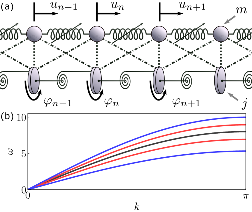
Figure 1: (a) Schematic of 1D lattice with two degrees of freedom modeled as a coupled lattice system with lumped mass $m$ and disc with rotational inertia $j$ The lumped masses are connected with nonlinear springs, and so are the discs. Adjacent masses and discs are connected with nonlinear springs as well, denoted as dashed and dash-dotted lines. (b) The dispersion relationship both with and without the coupling term $\alpha_{12}$. Black dashed line: $\alpha_{11}=\alpha_{22}=16$ and $\alpha_{12}=0$; red solid lines: $\alpha_{11}=20$, $\alpha_{22}=12$, and $\alpha_{12}=0$; blue solid lines: $\alpha_{11}=20$, $\alpha_{22}=12$, and $\alpha_{12}=8$.

The coupled lattice is governed by the following equations of motion,

$$m_{n}\ddot{u}_{n}=V_{1}^{\prime}(\Delta u_{n-1},\Delta\varphi_{n-1})-V_{1}^{\prime}(\Delta u_{n},\Delta\varphi_{n}),$$ (1a)

$$j_{n}\ddot{\varphi}_{n}=V_{2}^{\prime}(\Delta u_{n-1},\Delta\varphi_{n-1})-V_{2}^{\prime}(\Delta u_{n},\Delta\varphi_{n}),$$ (1b)

where $m_{n}$ and $j_{n}$ are the mass and rotational inertia of the axial and rotational component, respectively, $\Delta u_{n}=u_{n}-u_{n+1}$ and $\Delta\varphi_{n}=\varphi_{n}-\varphi_{n+1}$ are the axial and rotational strains, with $u_{n}$ and $\varphi_{n}$ being the axial displacement and angle of rotation of the $n$-th particle respectively. $V_{1}^{\prime}$ and $V_{2}^{\prime}$ are the general nonlinear force and torque terms determined by differentiating the total potential energy $V=V(\Delta u,\Delta\varphi)$ of the unit cell as follows,

$$V^{\prime}_{1}=\frac{\partial V}{\partial(\Delta u)},\quad V^{\prime}_{2}=\frac{\partial V}{\partial(\Delta\varphi)}.$$ (2)

Here, the total potential energy $V$ is a function of $\Delta u$ and $\Delta\varphi$, and therefore the Hamiltonian of this system is:

$$H=\sum_{n\in\mathbb{Z}}\left[\frac{1}{2}\left(m_{n}\dot{u}_{n}^{2}+j_{n}\dot{\varphi}_{n}^{2}\right)+V(\Delta u_{n},\Delta\varphi_{n})\right].$$ (3)

In the present work, we assume that the masses are identical ($m_{n}=m$ and $j_{n}=j$), and that the potential $V$ is a fourth order polynomial, which can be thought of as a Taylor expansion of an application specific potential (e.g., $V$ has the form of a power-law in the case of the precompressed granular crystal lattice Nesterenko (2001)). In particular, the total potential energy function $V$ considered here is:

$$V(x,y) =\frac{1}{2}\alpha_{11}x^{2}+\alpha_{12}xy+\frac{1}{2}\alpha_{22}y^{2}$$

$$~{}~{}~{}+\frac{1}{6}\alpha_{111}x^{3}+\frac{1}{2}\alpha_{112}x^{2}y+\frac{1}{2}\alpha_{122}xy^{2}+\frac{1}{6}\alpha_{222}y^{3}$$

$$~{}~{}~{}+\frac{1}{24}\alpha_{1111}x^{4}+\frac{1}{6}\alpha_{1112}x^{3}y+\frac{1}{4}\alpha_{1122}x^{2}y^{2}$$

$$~{}~{}~{}+\frac{1}{6}\alpha_{1222}xy^{3}+\frac{1}{24}\alpha_{2222}y^{4}.$$ (4)

In the above definition, we assumed non-dimensional parameters (note that we retained the same symbols for $u,~{}\varphi,~{}t$)

$$u_{n}\rightarrow\frac{u_{n}}{D_{0}},\quad\varphi_{n}\rightarrow\frac{R_{0}\varphi_{n}}{D_{0}},\quad t\rightarrow\omega_{0}t$$ (5)

where $D_{0}$ is the lattice constant, $R_{0}$ is the radius of the particle (i.e., of the disc in Fig. 1(a)), and $T_{0}=1/\omega_{0}=c\sqrt{m/a_{11}}$ is the characteristic time scale. The parameter $c$ is an arbitrary real constant such that $\alpha_{11}=c^{2}$ and can be set to any positive real values including $\alpha_{11}=4$, which we use in the following sections. The $a_{11}$ is the dimensional linear stiffness coefficient of the axial channel (see Supplementary Note 1 for how the non-dimensional coefficients $\alpha$ are related to the dimensional coefficients $a$). With this rescaling, the coupled equations of motion become

$$\ddot{u}_{n} =V_{1}^{\prime}(\Delta u_{n-1},\Delta\varphi_{n-1})-V_{1}^{\prime}(\Delta u_{n},\Delta\varphi_{n}),$$ (6a)

$$\ddot{\varphi}_{n} =V_{2}^{\prime}(\Delta u_{n-1},\Delta\varphi_{n-1})-V_{2}^{\prime}(\Delta u_{n},\Delta\varphi_{n}).$$ (6b)

III Multiple-scale expansion

To analytically explore the behavior of our coupled lattice, we employ asymptotic expansions accompanied with multiple-scale variables Huang et al. (1993); Charalampidis et al. (2018b); Chong and Kevrekidis (2018). We define the perturbation parameter $0<\epsilon\ll 1$ and use the perturbative decomposition

$$u_{n} =\epsilon\left[A_{1,0}+\left(A_{1,1}E_{n}+{\rm c.c.}\right)\right]$$

$$~{}~{}~{}+\epsilon^{2}\left[A_{2,0}+\left(A_{2,1}E_{n}+A_{2,2}E_{n}^{2}+{\rm c.c.}\right)\right]$$

$$~{}~{}~{}+\epsilon^{3}\left[A_{3,0}+\left(A_{3,1}E_{n}+A_{3,2}E_{n}^{2}+A_{3,3}E_{n}^{3}+{\rm c.c.}\right)\right],$$ (7a)

$$\varphi_{n} =\epsilon\left[B_{1,0}+\left(B_{1,1}E_{n}+{\rm c.c.}\right)\right]$$

$$~{}~{}~{}+\epsilon^{2}\left[B_{2,0}+\left(B_{2,1}E_{n}+B_{2,2}E_{n}^{2}+{\rm c.c.}\right)\right]$$

$$~{}~{}~{}+\epsilon^{3}\left[B_{3,0}+\left(B_{3,1}E_{n}+B_{3,2}E_{n}^{2}+B_{3,3}E_{n}^{3}+{\rm c.c.}\right)\right],$$ (7b)

where $E_{n}=E_{n}(t)=e^{i(kn-\omega t)}$, where $k$ and $\omega$ are the wave number and angular frequency, respectively and (c.c.) is the complex conjugate. The $A_{i,j}=A_{i,j}(\xi,\tau)$ and $B_{i,j}=B_{i,j}(\xi,\tau)$ are amplitude functions to be determined that depend on the slow scale variables in space $\xi=\epsilon(n-\lambda t)$ and in time $\tau=\epsilon^{2}t$ with $\lambda$ being the group velocity.

Substituting ansatz (7) into Eq. (6) and collecting the terms according to the order of $\epsilon$ yields the wave dispersion relationship $\omega=\omega(k)$ at order $\mathcal{O}(\epsilon^{1}E_{n}^{1})$,

$$\omega_{\pm}^{2}=2\left(\alpha_{11}+\alpha_{22}\pm\sqrt{\left(\alpha_{11}-\alpha_{22}\right)^{2}+(2\alpha_{12}\kappa)^{2}}\right)$$

$$\times\sin^{2}\left(\frac{k}{2}\right),$$ (8)

where $\kappa^{2}=R_{0}^{2}/r^{2}=m_{n}R_{0}^{2}/j_{n}$ is the normalized curvature (i.e., $r$ is a radius of gyration of the disc).

The wave dispersion relationship is shown in Fig. 1(b) for a few select sets of linear coefficients $\alpha_{11}$, $\alpha_{12}$, and $\alpha_{22}$. If we keep the coupling term $\alpha_{12}=0$ and set $\alpha_{22}\neq\alpha_{11}$, this results in two distinct curves denoted as red lines in Fig. 1(b). Similarly, if we let $\alpha_{11}\neq\alpha_{22}$, but now set $\alpha_{12}\neq 0$, the wave dispersion curves appears as two blue curves in Fig. 1(b).

At the order $\mathcal{O}(\epsilon^{2}E_{n}^{1})$, we obtain the group velocity $\lambda=d\omega/dk$,

$$\lambda=-\frac{1}{\omega_{\pm}}\left((\alpha_{11}+\alpha_{22})\pm\sqrt{\left(\alpha_{11}-\alpha_{22}\right)^{2}+(2\alpha_{12}\kappa)^{2}}\right)$$

$$\times\sin k.$$ (9)

Finally, at order $\mathcal{O}(\epsilon^{3}E_{n}^{1})$, nonlinear partial differential equations of $A_{1,1}$ and $B_{1,1}$ emerge,

$$i\partial_{\tau}A_{1,1}+\nu_{2}\partial_{\xi}^{2}A_{1,1}+\nu_{3}\partial_{\xi}^{2}B_{1,1}+\nu_{4}|A_{1,1}|^{2}A_{1,1}+\nu_{5}|B_{1,1}|^{2}B_{1,1}$$

$$~{}~{}~{}~{}~{}~{}~{}~{}~{}~{}~{}~{}+\nu_{6}|B_{1,1}|^{2}A_{1,1}+\nu_{7}|A_{1,1}|^{2}B_{1,1}+\nu_{8}B_{1,1}^{*}A_{1,1}^{2}+\nu_{9}A_{1,1}^{*}B_{1,1}^{2}=0,$$ (10a)

$$i\partial_{\tau}B_{1,1}+\mu_{2}\partial_{\xi}^{2}A_{1,1}+\mu_{3}\partial_{\xi}^{2}B_{1,1}+\mu_{4}|A_{1,1}|^{2}A_{1,1}+\mu_{5}|B_{1,1}|^{2}B_{1,1}$$

$$~{}~{}~{}~{}~{}~{}~{}~{}~{}~{}~{}~{}+\mu_{6}|B_{1,1}|^{2}A_{1,1}+\mu_{7}|A_{1,1}|^{2}B_{1,1}+\mu_{8}B_{1,1}^{*}A_{1,1}^{2}+\mu_{9}A_{1,1}^{*}B_{1,1}^{2}=0,$$ (10b)

where superscripts $(^{*})$ denote the complex conjugate, and $\nu$ and $\mu$ with subscripts are the real constant coefficients defined in terms of the coefficients $\alpha$ (see section 2 in the Supplementary Note for more details of the asymptotic expansion and section 3 therein for the detailed expressions of coefficients $\nu_{i},~{}\mu_{i}$). Note that Eq. (10) resembles a coupled-NLSE, such as the Manakov system Manakov (1973). Unlike the Manakov system, Eq. (10) is non-integrable for generic values of the coefficients $\nu$ and $\mu$.

IV Soliton Initial Data

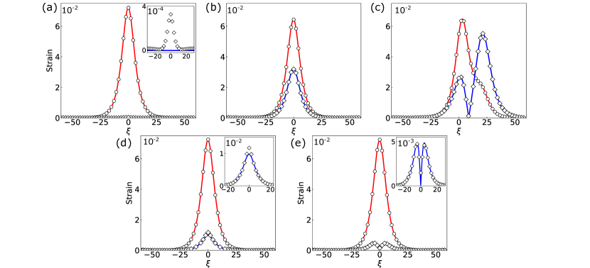
Figure 2: Coupled soliton solutions, which are analytically predicted (solid lines) and numerically computed for the full lattice equations and extracted at $\tau\approx 8$ (open symbols). (a) Initial data given by the single-component soliton of the two-component NLSE model, see Eq. (21) with $P_{1}=1,~{}P_{2}=0$, (b) Initial data given by the two-component soliton with different amplitudes, see Eq. (21) with $P_{1}=1,~{}P_{2}=0.5$, (c) Initial data given by the incoherently-coupled NLSE soliton with bimodal $b$ component, see Eq. (31), (d) Initial data given by the coherently-coupled NLSE soliton with unimodal $b$ component, see Eq. (36) with $m=0$, and (e) Initial data given by the coherently-coupled NLSE soliton with bimodal $b$ component, see Eq. (36) with $m=1$. The parameters are $\epsilon=0.09$, $\epsilon_{1}=0.027$, $q=0.1$, $q_{1}=0.1$, and $q_{2}=0.08$. Red solid lines and open circles correspond to the axial mode; blue solid lines and open squares correspond to the rotational mode. The markers are plotted for every 50 spatial points. The insets are zooms of the rotational modes.

To start our investigation, we first consider two special cases where Eqs. (10) reduce to well-known coupled NLSEs. In particular, we consider (i) the Manakov system and (ii) the coherently-coupled NLSE with energy exchange term. These special cases have exact solutions.

IV.1 Manakov Special Case

If we let all NLSE coefficients be zero except for $\nu_{2}$, $\mu_{3}$, $\nu_{4}$, $\nu_{6}$, $\mu_{7}$, and $\mu_{5}$, Eq. (10) reduces to the incoherently-coupled NLSE,

$$i\partial_{\tau}A_{1,1}+\nu_{2}\partial_{\xi}^{2}A_{1,1}+\left(\nu_{4}|A_{1,1}|^{2}+\nu_{6}|B_{1,1}|^{2}\right)A_{1,1}=0,$$ (11a)

$$i\partial_{\tau}B_{1,1}+\mu_{3}\partial_{\xi}^{2}B_{1,1}+\left(\mu_{7}|A_{1,1}|^{2}+\mu_{5}|B_{1,1}|^{2}\right)B_{1,1}=0.$$ (11b)

The above equations are generally non-integrable except for a few special sets of coefficients Haelterman et al. (1993); Haelterman and Sheppard (1994a, b). One of these is the well known Manakov system Manakov (1973). In this section, we consider the Manakov system with the coefficients $\nu_{2}=\mu_{3}=1/2$ and $\nu_{4}=\nu_{6}=\mu_{7}=\mu_{5}=1$, which has exact solutions of the form,

$$\left(\begin{array}[]{ccccccccccccccc}A_{1,1}(\xi,\tau)\\ B_{1,1}(\xi,\tau)\end{array}\right)=\left(\begin{array}[]{ccccccccccccccc}a(\xi)\\ b(\xi)\end{array}\right)e^{i2q^{2}\tau},$$ (16)

where the envelopes $a$ and $b$ are real valued functions (without loss of generality in the 1-dimensional case considered herein), and $q$ is a real parameter associated with the wave frequency. Among the many possible solutions of this form, we consider here the fundamental (bright) one-soliton solutions Manakov (1973); Ablowitz et al. (2003),

$$\left(\begin{array}[]{ccccccccccccccc}a(\xi)\\ b(\xi)\end{array}\right)=\frac{2q}{\sqrt{P_{1}^{2}+P_{2}^{2}}}\left(\begin{array}[]{ccccccccccccccc}P_{1}\\ P_{2}\end{array}\right)\operatorname{sech}(2q\xi).$$ (21)

Alternatively, if we assume

$$\left(\begin{array}[]{ccccccccccccccc}A_{1,1}(\xi,\tau)\\ B_{1,1}(\xi,\tau)\end{array}\right)=\left(\begin{array}[]{ccccccccccccccc}a(\xi)e^{i2q_{1}^{2}\tau}\\ b(\xi)e^{i2q_{2}^{2}\tau}\end{array}\right),$$ (26)

where two different real frequency parameters $q_{1}$ and $q_{2}$ exist, Eq. (11) allows the multi-hump soliton solutions Stalin et al. (2019); Ramakrishnan et al. (2020),

$$\left(\begin{array}[]{ccccccccccccccc}a(\xi)\\ b(\xi)\end{array}\right)= \frac{2}{F(\xi)}\left[\left(\begin{array}[]{ccccccccccccccc}P_{1}e^{2q_{1}\xi}\\ P_{2}e^{2q_{2}\xi}\end{array}\right)\right.$$ (31)

$$~{}~{}~{}~{}\left.+g\left(\begin{array}[]{ccccccccccccccc}P_{2}q_{1}^{2}e^{2q_{2}\xi}\\ -P_{1}q_{2}^{2}e^{2q_{1}\xi}\end{array}\right)e^{2(q_{1}+q_{2})\xi}\right]$$ (34)

where $P_{1}$ and $P_{2}$ are the arbitrary amplitude parameters, $F(\xi)=\frac{P_{1}^{2}}{4q_{1}^{2}}e^{4q_{1}\xi}+\frac{P_{2}^{2}}{4q_{2}^{2}}e^{4q_{2}\xi}+\frac{P_{1}^{2}P_{2}^{2}\left(q_{1}-q_{2}\right)^{2}}{16q_{1}^{2}q_{2}^{2}\left(q_{1}+q_{2}\right)^{2}}e^{4\left(q_{1}+q_{2}\right)\xi}$, and $g=[P_{1}P_{2}\left(q_{1}-q_{2}\right)]/[(2q_{1}q_{2})^{2}\left(q_{1}+q_{2}\right)]$.

IV.2 coherently-coupled NLSE System

Another interesting example where solitary wave solutions can be identified is by setting the coefficients $\nu_{3},~{}\nu_{5},~{}\nu_{7},~{}\nu_{8}$ and $\mu_{2},~{}\mu_{4},~{}\mu_{6},~{}\mu_{9}$ of Eq. (10) to zero. Under such a selection, Eq. (10) reduces to the coherently-coupled NLSE Kivshar and Agrawal (2003) with the form:

$$i\partial_{\tau}A_{1,1}+\nu_{2}\partial_{\xi}^{2}A_{1,1}$$

$$~{}~{}~{}+\left(\nu_{4}|A_{1,1}|^{2}+\nu_{6}|B_{1,1}|^{2}\right)A_{1,1}+\nu_{9}A_{1,1}^{*}B_{1,1}^{2}=0,$$ (35a)

$$i\partial_{\tau}B_{1,1}+\mu_{3}\partial_{\xi}^{2}B_{1,1}$$

$$~{}~{}+\left(\mu_{7}|A_{1,1}|^{2}+\mu_{5}|B_{1,1}|^{2}\right)B_{1,1}+\mu_{8}B_{1,1}^{*}A_{1,1}^{2}=0.$$ (35b)

Once again, this is a model that frequently arises in nonlinear optics in the realm of processes such as four-wave mixing and a systematic derivation of such models can be found, e.g., in Kivshar and Agrawal (2003).

When $\nu_{2}=\mu_{3}=1/2$ and $\nu_{4}=\mu_{5}=1$, this system also has solutions of the form given by Eq. (16) Kivshar and Agrawal (2003); Haelterman et al. (1993); Haelterman and Sheppard (1994a, b), but now the amplitudes are only approximations,

$$a(\xi)= 2q\operatorname{sech}(2q\xi),$$ (36a)

$$b(\xi)\approx \epsilon_{1}\sqrt{1-G(\xi)^{2}}{}_{2}F_{1}\left(-m,m+3,2,\frac{1-G(\xi)}{2}\right).$$ (36b)

Here, $0<\epsilon_{1}\ll 1$ is another perturbation parameter, $G(\xi)=\tanh(2q\xi)$, and ${}_{2}F_{1}$ is a hypergeometric function. In this expression, as is discussed in Kivshar and Agrawal (2003), $m$ is a non-negative integer, and for each distinct corresponding value a different branch of vector solitons exists. With the constraint that $m$ is an integer, in order for $m$-th order solitons to exist, the NLSE coefficients require the following relations, $\nu_{9}=(m+1)(m+2)-\nu_{6},\quad\mu_{9}=(m+1)(m+2)-\mu_{7}$.

IV.3 Numerical simulations of coupled solitons

Figure 2 shows a comparison of analytical and numerical soliton solutions of axial and rotational components. The lattice model initialized with various soliton solutions of the special cases considered above is numerically solved in the domain $\xi\in[-150,150]$ and $\tau\in[0,10]$ with perturbation parameter $\epsilon=0.09$. Spatial profiles of the analytical and numerical solutions are extracted at $\tau=8$ (i.e., $t\approx 987.7$), and plotted as solid lines and open symbols, respectively. For the Manakov case, we used the coefficient values: $\alpha_{11}=\alpha_{22}=4$, $\alpha_{111}=-1$, $\alpha_{112}=\alpha_{122}=\alpha_{222}=\alpha_{1122}=\alpha_{1222}=1$, $\alpha_{1112}=\alpha_{2222}=2$, and $\alpha_{12}=\alpha_{1112}=0$. For the coherently-coupled case, we used: for $n=0$, $\alpha_{11}=\alpha_{22}=4$, $\alpha_{11}=\alpha_{22}=3$, $\alpha_{112}=1$, $\alpha_{1111}=6$, $\alpha_{1112}=\alpha_{1122}=3/2$, $\alpha_{2222}=11/2$, and $\alpha_{12}=\alpha_{122}=\alpha_{1112}=0$. For $n=1$, $\alpha_{11}=\alpha_{22}=4$, $\alpha_{111}=3$, $\alpha_{222}=19$, $\alpha_{112}=1$, $\alpha_{1111}=6$, $\alpha_{1112}=3/2$, $\alpha_{1122}=11/2$, $\alpha_{2222}=363/2$, and $\alpha_{12}=\alpha_{122}=\alpha_{1112}=0$. In general, both numerically solved axial and rotational components agree well overall with the analytical approximation, regardless of the initial condition or the choice of coefficients. There are however, also deviations between the prediction and the actual dynamics, which is to be expected, given the approximate nature of the reduction. For example, there exists a small non-zero solution in the rotational component in Fig. 2(a) (see inset figure), despite initializing the lattice with a single-component solitary wave. This suggests that there is a weak energy leakage from the axial channel (with non-zero initial data) to the rotational channel (with zero initial data). However, given that the spatial profile in rotational mode is very small in amplitude, the relevant energy transfer is rather minimal.

When we have non-zero amplitude initial data in both axial and rotational components (Fig. 2(b-e)), we see a good agreement with the analytical prediction, even for the case where either or both the axial and rotational component initial condition is asymmetric rather than unimodal (Fig. 2(c) and (e)). There exist some slight disparities in the coherently-coupled NLSE case (i.e., Fig. 2(d-e)), presumably due to the stronger coupling in coherently-coupled case. Nevertheless, the overall agreement is excellent, regardless of the initial condition profile.

V Rogue Wave Initial Data

Next, we consider solutions that are spatio-temporally localized, namely the rogue wave solutions of the two-component NLSE system (Eq. (11)). Again, the NLSE coefficient $\nu_{2}=\mu_{3}=1/2$ and $\nu_{4}=\nu_{6}=\mu_{7}=\mu_{5}=1$ are chosen (i.e., the Manakov system).

One of the fundamental rogue wave solutions of the Manakov system Baronio et al. (2012) is given by

$$\left(\begin{array}[]{ccccccccccccccc}A_{1,1}(\xi,\tau)\\ B_{1,1}(\xi,\tau)\end{array}\right)=\left[L\left(\begin{array}[]{ccccccccccccccc}P_{1}\\ P_{2}\end{array}\right)+M\left(\begin{array}[]{ccccccccccccccc}P_{2}\\ -P_{1}\end{array}\right)\right]\frac{e^{i4q^{2}\tau}}{B},$$ (43)

where $a$ and $b$ are arbitrary real parameters, the real frequency parameter is $q=\sqrt{P_{1}^{2}+P_{2}^{2}}$, $L=\frac{3}{2}-32q^{4}\tau^{2}-8q^{2}\xi^{2}+i16q^{2}\tau+|f|^{2}e^{4q\xi}$, $M=4f(2q\xi-i4q^{2}\tau-\frac{1}{2})e^{2q\xi+i2q^{2}\tau}$, and $B=\frac{1}{2}+32q^{4}\tau^{2}+8q^{2}\xi^{2}+|f^{2}|e^{4q\xi}$ with $f$ being an arbitrary complex parameter.

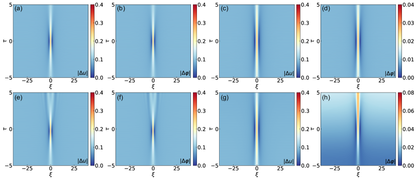
Figure 3: Coupled rogue wave solutions, which are analytically predicted (top row) and numerically solved for the full lattice equations initialized with Eq. (43) (bottom row). The perturbation parameter is $\epsilon=0.09$, and the amplitudes are (a,b,e,f) $P_{1}=P_{2}=0.2$, $f=0$, and (c,d,g,h) $P_{1}=0.2$, $P_{2}=0.02$, and $f=0$.

Setting $f=0$, we obtain coupled vector solutions in the axial and rotational components that are reminiscent of the Peregrine soliton. We consider two case examples. One where the axial and rotational components are chosen to be identical (i.e., effectively the single component situation), see Fig. 3(a) and (b). We also consider a case example where the rotational component is $1/10$ of the amplitude of the axial component, see Fig. 3(c) and (d). In both cases, the peak amplitude is three times higher than the background and is localized at the origin. There are also density dips in the vicinity of the principal peak.

Using the spatial profile at $\tau=-5$ from the NLSE approximation as initial data, we simulate the lattice dynamics in the domain $\tau\in[-5,5]$ and $\xi\in[-40,40]$. The perturbation parameter is set to $\epsilon=0.09$, and we choose the following coefficients: $\alpha_{11}=\alpha_{22}=4$, $\alpha_{122}=\sqrt{2}$, $\alpha_{1111}=\alpha_{1122}=1$, $\alpha_{2222}=2$, and $\alpha_{12}=\alpha_{111}=\alpha_{112}=\alpha_{222}=\alpha_{1112}=\alpha_{1222}=\alpha_{1222}=0$. The resulting numerical solutions are shown in Fig. 3(e-h). In both components, the time until the localization coincides well with the analytical prediction, however there are slight discrepancies after the formation of the rogue wave (i.e., $\tau>0$). In particular, the peak formed at the origin splits into smaller amplitude waves in the lattice case. Similar observations have been made in other lattice settings Charalampidis et al. (2018b). As discussed in Ref. Charalampidis et al. (2018b), the formation of smaller waves may be induced by the modulational instability of the NLSE background, which is activated due to the large peak amplitude.

In Fig. 3(g-h) where the axial and rotational component have different amplitudes, the waves tend to focus and thus localize at the origin. In the axial component, we see that the peak amplitude of the numerical solution is slightly lower than the analytical prediction. On the contrary, the rotational component shows a peak that is twice as high as the analytical prediction. The deviation from the analytical prediction suggests there is energy leakage from the axial component into the rotational component (see Supplementary Note 4 for longer time spatio-temporal evolution and how it differs from analytical prediction). We believe that this is due to the non-zero coupling terms of the lattice equation (e.g., $\alpha_{122}$), which possibly trigger the energy transfer between two components, in a way that is not reflected in the reduced NLSE system.

VI Gaussian Initial Data

To further explore rogue wave solutions in the coupled lattice, we hereafter numerically study Eq. (10) in the more general case (i.e., with all coefficients being present). However, as mentioned previously, Eq. (10) is non-integrable, therefore no exact Peregrine-like solution is analytically known. Thus, the lattice cannot be initialized with an analytical prediction to examine the time evolution. As an alternative, we consider more general unimodal shaped data. In particular, we use the Gaussian initialization, which has been shown to be effective in leading to rogue-like waves as a result of the gradient catastrophe phenomenon in the focusing NLSE Bertola and Tovbis (2013). This has been mathematically explored originally in the so-called semi-classical continuum NLSE system in the work Bertola and Tovbis (2013), and more recently explored in corresponding experimental studies in nonlinear optics in the work of Tikan et al. (2017).

Let the initial data be the Gaussian envelope function Charalampidis et al. (2018b),

$$\left(\begin{array}[]{ccccccccccccccc}A_{1,1}(\xi,\tau=0)\\ B_{1,1}(\xi,\tau=0)\end{array}\right)=\left(\begin{array}[]{ccccccccccccccc}P_{1}\\ P_{2}\end{array}\right)\exp\left(-\frac{\xi^{2}}{4\sigma^{2}}\right),$$ (48)

where $P_{1}$ and $P_{2}$ are arbitrary real parameters that determine the amplitude of the initial profile of $A_{1,1}$ and $B_{1,1}$ respectively, and $\sigma$ is the width of the localization. The numerical simulation is then conducted in the domain $\tau\in[0,5]$ and $[0,20]$, and $\xi\in[-30,30]$ with the perturbation parameter $\epsilon=0.09$. The lattice coefficients are set to: $\alpha_{11}=\alpha_{22}=16$, $\alpha_{12}=0.016$, $\alpha_{111}=\alpha_{222}=\alpha_{1111}=\alpha_{1112}=\alpha_{1122}=\alpha_{1222}=\alpha_{2222}$, and $\alpha_{112}=\alpha_{122}=1.6$. Here, these choices are made such that the NLSE becomes the focusing equation (i.e., $\nu_{i}>0$ and $\mu_{i}>0$). The corresponding simulations of the NLSE (Eq. (10)) are also conducted as a reference solution to be compared with the lattice dynamics solutions.

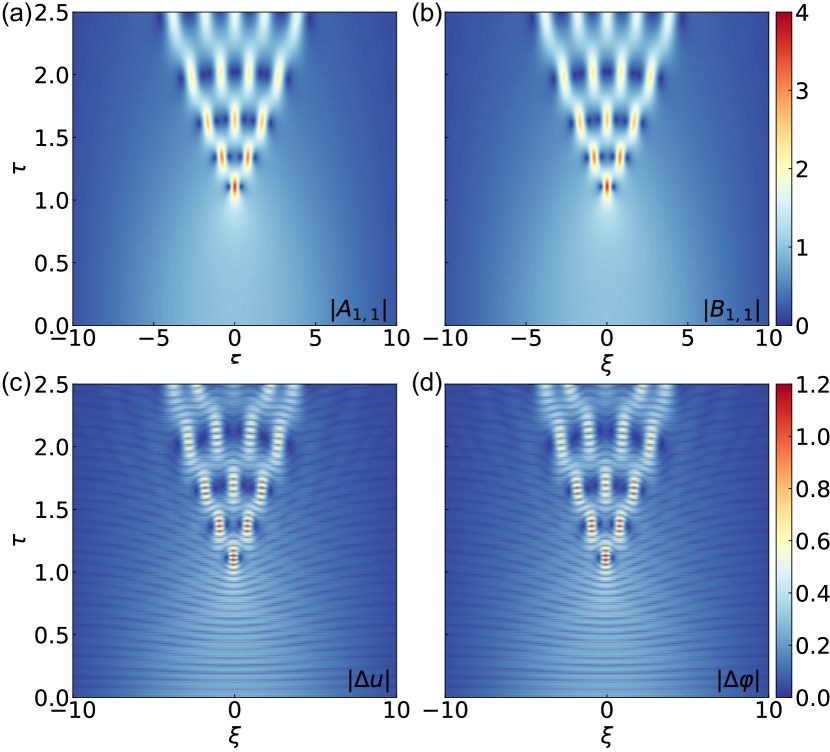
Figure 4: Numerical solutions of NLSE (top row) and of the lattice (bottom row) with all coefficients in Eq. (10) being non-zero. The perturbation parameter is $\epsilon=0.09$, the width of the localization is $\sigma=4$, and the amplitudes are $P_{1}=P_{2}=1.0$.

Figures 4 and 5 show both lattice and NLSE simulation results for two different cases of initial conditions. Specifically, (i) the initial condition where axial and rotational modes have equal amplitude (i.e., $P_{1}=P_{2}=1.0$; Fig. 4), and (ii) the initial condition with the rotational mode being $1/10$ of axial mode (i.e., $P_{1}=1.0$, $P_{2}=0.1$; Fig. 5) to examine how the energy transfer differs between the lattice and the NLSE simulation. The localization width $\sigma=4$ is kept constant between the two cases.

First, if we use the equal amplitude initial conditions, the NLSE creates a tree-like pattern stemming from single peak localization at $\tau\approx 1.1$. This is in line with the integrable NLSE theory of Bertola and Tovbis (2013) and has also been observed in other systems, both continuum Charalampidis et al. (2018a) and discrete Charalampidis et al. (2018b). The single peak localization has dips on the left and right side, which are directly reminiscent of a Peregrine soliton. In the lattice simulation, we also see the tree-like pattern starting from the peak at $\tau\approx 1.1$. As can be observed, the branches formed after $\tau\approx 2$ show small differences between the lattice simulation and the NLSE (e.g., the two center peaks are formed slightly later in the lattice spatio-temporal evolution compared to the NLSE and the peak amplitude is different. However, in general, the NLSE and lattice behave in a fairly similar manner, especially from the standpoint of the time at which the wave localizes in the early stage of the time evolution, the formation of the original Peregrine pattern, and also the tree-like pattern that follows.

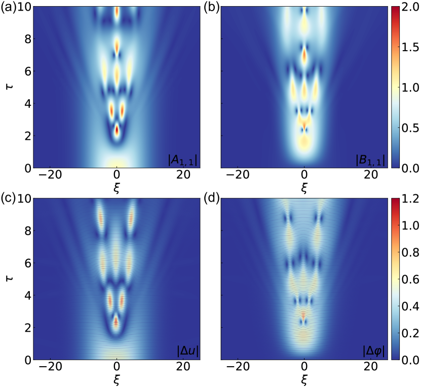
Figure 5: Numerical solutions of NLSE (a,b) and lattice (c,d) with all coefficients in Eq. (10) being non-zero. Perturbation parameter is $\epsilon=0.2$, width of the localization is $\sigma=4$, and the amplitudes are $P_{1}=1.0,~{}P_{2}=0.1$.

Similarly, if we employ a smaller amplitude initial condition in the rotational mode, the NLSE and the lattice well agree in their spatio-temporal profiles. In the NLSE simulation, the axial component (Fig. 5(a)), wide Gaussian initial data first decreases and then forms teardrop-like peak at $\tau\approx 2.25$. This single peak split into two peaks at $\tau\approx 3.5$, then into three. However, unlike the case with equal amplitude initial condition, the profile does not develop into tree-like pattern. Instead, a more localized pattern centered around $\xi=0$ forms. As for the rotational component of the NLSE shown in Fig. 5(b), in constrast to the axial component, the amplitude first increases and reaches its highest amplitude at $\tau\approx 1.5$ while keeping the broad width of the Gaussian initial profile. Then, the peak narrows as two dips appear at $\tau\approx 2.25$, where the axial component forms a single peak. As time proceeds, we can observe two small and narrow peaks accompanied by adjacent dips that emerge at $\tau\approx 3.5$. In the lattice solution, we can observe similar dynamics. For instance, the axial component forms a teardrop-like peak at $\tau\approx 2.3$ while the rotational component shows two dips with a very narrow peak at $\xi=0$. However, as we also observe in the equal amplitude initial data case, the spatio-temporal evolution of the lattice starts to deviate from the NLSE behavior as time proceeds. After $\tau\approx 6$ the pattern formations (e.g., number of peaks) of the lattice deviate from those of NLSE.

VII Energy exchange

In this section, we revisit the soliton and rogue wave solutions of the lattice simulation studied in the previous sections, and examine the energy profiles in the axial and rotational modes as a function of time. We split the energy into two groups, (i) axial component and (ii) rotational components as follows:

$$E_{1} =\frac{1}{2}\dot{u}^{2}+\frac{1}{2}\alpha_{11}u^{2}+\frac{1}{6}\alpha_{111}u^{3}+\frac{1}{24}\alpha_{1111}u^{4}+\frac{1}{2}E_{cp},$$ (49a)

$$E_{2} =\frac{1}{2}\dot{\varphi}^{2}+\frac{1}{2}\alpha_{22}\varphi^{2}+\frac{1}{6}\alpha_{222}\varphi^{3}+\frac{1}{24}\alpha_{2222}\varphi^{4}+\frac{1}{2}E_{cp},$$ (49b)

$$E_{cp} =\alpha_{12}u\varphi+\frac{1}{2}\alpha_{112}u^{2}\varphi+\frac{1}{2}\alpha_{122}u\varphi^{2}$$

$$~{}~{}~{}+\frac{1}{6}\alpha_{1112}u^{3}\varphi+\frac{1}{4}\alpha_{1122}u^{2}\varphi^{2}+\frac{1}{6}\alpha_{1222}u\varphi^{3}.$$ (49c)

Note that we evenly distribute the energy due to coupling terms $E_{cp}$ among $E_{1}$ and $E_{2}$. We investigate these two energy quantities for the solitary, rogue, and Gaussian induced wave solutions shown in Fig. 2, Fig. 3, and Fig. 5 respectively. Figure 6 shows the energy of the axial and rotational component of different cases of the lattice simulation.

First, we take a closer look at the soliton solution case shown in Fig. 6(a) and (b), which corresponds to the soliton solutions shown in Fig. 2(a) and (c) respectively. In general, both soliton solution energy profiles suggest that the energy does not transfer from one mode to another (i.e., $E_{1}$ and $E_{2}$ are constant throughout), except for the minimal leakage seen in the inset plot of Fig. 6(a). This energy leakage can also be seen in the spatial profile in Fig. 2(a), where the rotational mode profile has a very small peak at the center. The energy in the rotational mode rapidly increases from zero and then saturates, in this case around $E_{2}/E_{t}=2.5\times 10^{-5}$. Indeed, the stationary nature of the solution preserves the dynamics essentially thereafter. Although we set the leading order coupling term $\alpha_{12}=0$, the lattice of interest is still coupled at higher orders (e.g., $\alpha_{112}u^{2}$ or $\alpha_{1112}u^{3}$). Therefore, with non-zero axial amplitude $u$, the rotational mode is excited, and effectively the axial mode plays the role of an external potential of the small amplitude, leading to practically linear dynamics in the rotational mode. Nonetheless, the energy leakage remains minimal in this case. The profiles in Fig. 6(b) also suggest the suppression of energy leakage since the energy profiles are almost constant, with minimal energy leakage from the axial to rotational the component. In the inset panel of Fig. 6(b), we see that the deviation from the initial value $\frac{E_{2}-E_{2}(0)}{E_{t}}$ is quite small ($\approx 5\times 10^{-5}$) and practically negligible.

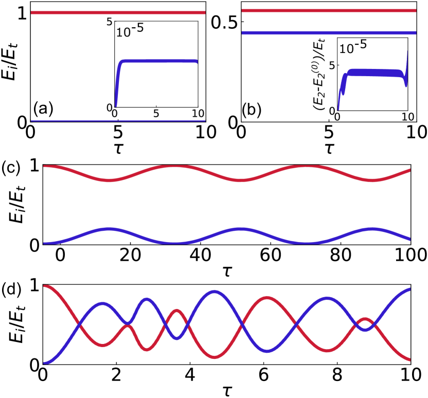
Figure 6: Energy profiles of axial $E_{1}$ and rotational $E_{2}$ component of the lattice, normalized by the total energy $E_{t}$. Red solid lines, axial component $E_{1}$; blue solid lines, rotational component $E_{2}$. Each panel corresponds to the soliton solutions: (a) Fig. 2(a), (b): Fig. 2(c), and rogue wave solutions (c): Fig. 3(g-h), and Gaussian initial data solutions (d): Fig. 5(c-d). The inset panel in: (a) represents a magnified view of the rotational mode in $\tau\in[0,10]$; (b) represents the deviation from the initial energy in rotational component, $[E_{2}-E_{2}(0)]/E_{t}$.

In Fig. 6(c) we show the time evolution of the energy component of the coupled rogue wave solution, which corresponds to the strain wave field in Fig. 3(g,h), but with $\tau=35$. We observe a continuous and gradual exchange of energy between the two channels. As time progresses, the energy distributed to the rotational component grows and reaches its maximum, which is about 1/4 of the energy in axial component at $\tau\approx 14$. Then, $E_{2}$ decreases and attains a minimum at $\tau\approx 32$. Even in the longer term behavior, this gradual and partial exchange of the energy continues in a recurrent manner (see also Supplementary Note 4 for the spatio-temporal evolution).

Lastly, we explore the energy exchange between the axial and rotational components of the rogue wave-like solutions induced by Gaussian initial data, shown in Fig. 6(d), which correspond to the strain wave field in Fig. 5. Unlike the above three cases, we see significant energy transfer between the two components. As observed in the spatio-temporal evolution of the lattice solution, the axial and rotational component exchange a significant amount of energy quite quickly. Indeed the rotational component of the energy $E_{2}$ overtakes the axial component at $\tau\approx 1.6$. When the first peak forms in the axial component of the lattice simulation ($\tau\approx 2.3$; a narrow peak forms in rotational component), we see that the two energy components become almost identical. Interestingly, even after the single peak formation, when the spatio-temporal profile of the lattice shows peaks, the difference between the two energy component becomes small. For instance, two energy components essentially become identical again, when two peaks become significantly high in amplitude at $\tau\approx 3.9$ in the axial component (two narrow peaks form in the rotational component). Similar behavior can also be observed at $\tau\approx 6.9$ and $\tau\approx 9$.

In summary, we observe three qualitatively different types of behavior of energy transfer. For solitary wave initial data, there is minimal transfer of energy. For Peregrine initial data, there is a partial transfer of energy between channels, and for Gaussian initial data, the energy is transferred continuously between the two channels in an aperiodic and oscillatory fashion.

VIII Conclusions and Future Work

In conclusion, we have analytically and numerically explored nonlinear waves in a FPUT lattice with axial and rotational modes involving up to cubic stiffness. We first derived coupled NLSE equations via a multiple-scale analysis. Variants of both incoherently-coupled and coherently-coupled forms were considered and used to approximate the full lattice dynamics. The approximation based on the solitary wave solution of the incoherently-coupled NLSE compared favorably to the numerical simulation of the coupled FPUT lattice, both with and without energy exchange terms. In the coherently-coupled NLSE case, we also explored more complex waveforms in addition to the simplest unimodal solitary wave (where one component played the role of an effective potential for the other). Furthermore, rogue wave type dynamics were studied. First we used the exact coupled rogue wave solution of the incoherently-coupled NLSE system (i.e., Manakov system), as the initial condition. Regardless of the initial profile, the localization time of the analytical and numerical solution matched well, except for the small but noticeable energy leakage from the axial component to the rotational component. When initialized with a sufficiently wide Gaussian envelope function, the lattice showed a clear localization due to the gradient catastrophe phenomenon, accompanied by the formation of secondary peaks, in line with a similar phenomenology previously analyzed in the NLSE realm. Depending on the configuration and the initial data, coupled lattices of the FPUT type considered herein can effectively isolate the energy (e.g., soliton solutions) to one of the modes or continuously exchange the energy between modes while forming a peak (e.g., Gaussian initial data solutions).

We believe that these findings open an analytical window of investigation of a multitude of systems that have recently been explored in various experiments at the multi-component setting Yasuda et al. (2019); Deng et al. (2018, 2019). This allows one to observe wave localization in a general coupled discrete nonlinear system, and may, in principle, open avenues to explore energy control in mechanical systems. At the same time, while here we presented the relevant multi-component technique at the one-dimensional, two-component setting, there are various recent works that suggest the relevance of corresponding considerations for higher numbers of components Deng et al. (2019) or higher dimensions Chong et al. (2021).

References

- Kharif and Pelinovsky (2003) C. Kharif and E. Pelinovsky, European Journal of Mechanics, B/Fluids 22, 603 (2003).
- Haver (2004) S. Haver, Rogue waves 2004 : proceedings of a workshop organized by Ifremer and held in Brest, France 2004, 1 (2004).
- Walker et al. (2004) D. A. Walker, P. H. Taylor, and R. E. Taylor, Applied Ocean Research 26, 73 (2004).
- Adcock et al. (2011) T. A. Adcock, P. H. Taylor, S. Yan, Q. W. Ma, and P. A. Janssen, Proceedings of the Royal Society A: Mathematical, Physical and Engineering Sciences 467, 3004 (2011).
- Mori and Liu (2002) N. Mori and P. C. Liu, Ocean Engineering 29, 1399 (2002).
- Baschek and Imai (2011) B. Baschek and J. Imai, Oceanography 24, 158 (2011).
- Pelinovsky and Kharif (2016) E. Pelinovsky and C. Kharif, Extreme Ocean Waves (Springer International Publishing, Cham, 2016) pp. 1–236.
- Chabchoub et al. (2011) A. Chabchoub, N. P. Hoffmann, and N. Akhmediev, Physical Review Letters 106, 204502 (2011).
- Chabchoub et al. (2012) A. Chabchoub, N. Hoffmann, M. Onorato, and N. Akhmediev, Physical Review X 2, 2 (2012).
- McAllister et al. (2018) M. L. McAllister, S. Draycott, T. A. Adcock, P. H. Taylor, and T. S. Van Den Bremer, Journal of Fluid Mechanics 860, 767 (2018).
- Xu et al. (2020) G. Xu, A. Chabchoub, D. E. Pelinovsky, and B. Kibler, Physical Review Research 2, 33528 (2020).
- Charalampidis et al. (2018a) E. G. Charalampidis, J. Cuevas-Maraver, D. J. Frantzeskakis, and P. G. Kevrekidis, Romanian Reports in Physics 70, 1 (2018a), arXiv:1609.01798 .
- Solli et al. (2007) D. R. Solli, C. Ropers, P. Koonath, and B. Jalali, Nature 450, 1054 (2007).
- Dudley et al. (2014) J. M. Dudley, F. Dias, M. Erkintalo, and G. Genty, Nature Photonics 8, 755 (2014).
- Frisquet et al. (2016) B. Frisquet, B. Kibler, P. Morin, F. Baronio, M. Conforti, G. Millot, and S. Wabnitz, Scientific Reports 6, 1 (2016).
- Tikan et al. (2017) A. Tikan, C. Billet, G. El, A. Tovbis, M. Bertola, T. Sylvestre, F. Gustave, S. Randoux, G. Genty, P. Suret, and J. M. Dudley, Physical Review Letters 119, 33901 (2017).
- Höhmann et al. (2010) R. Höhmann, U. Kuhl, H. J. Stöckmann, L. Kaplan, and E. J. Heller, Physical Review Letters 104, 1 (2010), arXiv:0909.0847 .
- Ruderman (2010) M. S. Ruderman, European Physical Journal: Special Topics 185, 57 (2010).
- Sabry et al. (2012) R. Sabry, W. M. Moslem, and P. K. Shukla, Physics of Plasmas 19 (2012), 10.1063/1.4772058.
- Bains et al. (2014) A. S. Bains, B. Li, and L. D. Xia, Physics of Plasmas 21 (2014), 10.1063/1.4869464, arXiv:1403.3745 .
- Tolba et al. (2015) R. E. Tolba, W. M. Moslem, N. A. El-Bedwehy, and S. K. El-Labany, Physics of Plasmas 22 (2015), 10.1063/1.4918706.
- Onorato et al. (2013) M. Onorato, S. Residori, U. Bortolozzo, A. Montina, and F. T. Arecchi, “Rogue waves and their generating mechanisms in different physical contexts,” (2013).
- R. Osborne (2010) A. R. Osborne, Nonlinear Ocean Wave and the Inverse Scattering Transform (Elsevier, Amsterdam, 2010).
- Sulem and Sulem (1999) C. Sulem and P. Sulem, The Nonlinear Schrödinger Equation: Self-Focusing and Wave Collapse (Springer-Verlag New York, 1999).
- Ablowitz et al. (2003) M. J. Ablowitz, B. Prinari, and A. D. Trubatch, Discrete and Continuous Nonlinear Schrödinger Systems (Cambridge University Press, 2003).
- Peregrine (1983) D. H. Peregrine, The Journal of the Australian Mathematical Society. Series B. Applied Mathematics 25, 16 (1983).
- Charalampidis et al. (2018b) E. G. Charalampidis, J. Lee, P. G. Kevrekidis, and C. Chong, Physical Review E 98, 1 (2018b), arXiv:1801.06086 .
- Akhmediev and Ankiewicz (2011) N. Akhmediev and A. Ankiewicz, Physical Review E - Statistical, Nonlinear, and Soft Matter Physics 83, 1 (2011).
- Ankiewicz et al. (2010) A. Ankiewicz, N. Akhmediev, and J. M. Soto-Crespo, Physical Review E - Statistical, Nonlinear, and Soft Matter Physics 82 (2010), 10.1103/PhysRevE.82.026602.
- Wen and Wang (2018) X. Y. Wen and D. S. Wang, Wave Motion 79, 84 (2018).
- Yan and Jiang (2012) Z. Yan and D. Jiang, Journal of Mathematical Analysis and Applications 395, 542 (2012).
- Maluckov et al. (2013) A. Maluckov, N. Lazarides, G. P. Tsironis, and L. Hadžievski, Physica D: Nonlinear Phenomena 252, 59 (2013), arXiv:1204.5303 .
- Hoffmann et al. (2018) C. Hoffmann, E. G. Charalampidis, D. J. Frantzeskakis, and P. G. Kevrekidis, Physics Letters, Section A: General, Atomic and Solid State Physics 382, 3064 (2018).
- Sullivan et al. (2020) J. Sullivan, E. Charalampidis, J. Cuevas-Maraver, P. Kevrekidis, and N. Karachalios, European Physical Journal Plus 135, 607 (2020).
- Han et al. (2014) D. Han, M. Westley, and S. Sen, Physical Review E - Statistical, Nonlinear, and Soft Matter Physics 90, 1 (2014).
- Kashyap and Sen (2021) R. Kashyap and S. Sen, arXiv preprint arXiv:2105.05028 (2021).
- Merkel et al. (2011) A. Merkel, V. Tournat, and V. Gusev, Physical Review Letters 107 (2011), 10.1103/PhysRevLett.107.225502.
- Pichard et al. (2014) H. Pichard, A. Duclos, J. P. Groby, V. Tournat, and V. E. Gusev, Physical Review E - Statistical, Nonlinear, and Soft Matter Physics 89, 13201 (2014).
- Köpfler et al. (2019) J. Köpfler, T. Frenzel, M. Kadic, J. Schmalian, and M. Wegener, Physical Review Applied 11, 34059 (2019).
- Ngapasare et al. (2020) A. Ngapasare, G. Theocharis, O. Richoux, C. Skokos, and V. Achilleos, Physical Review B 102, 54201 (2020).
- Allein et al. (2017) F. Allein, V. Tournat, V. E. Gusev, and G. Theocharis, Extreme Mechanics Letters 12, 65 (2017), arXiv:1607.00831 .
- Dubus et al. (2016) B. Dubus, N. Swinteck, K. Muralidharan, J. O. Vasseur, and P. A. Deymier, Journal of Vibration and Acoustics, Transactions of the ASME 138 (2016), 10.1115/1.4033457.
- Deng et al. (2018) B. Deng, P. Wang, Q. He, V. Tournat, and K. Bertoldi, Nature Communications 9, 1 (2018).
- Zhang et al. (2019) Q. Zhang, O. Umnova, and R. Venegas, Physical Review E 100, 062206 (2019).
- Yasuda et al. (2019) H. Yasuda, Y. Miyazawa, E. G. Charalampidis, C. Chong, P. G. Kevrekidis, and J. Yang, Science Advances 5, 1 (2019), arXiv:1805.05909 .
- Deng et al. (2019) B. Deng, C. Mo, V. Tournat, K. Bertoldi, and J. R. Raney, Physical Review Letters 123, 24101 (2019).
- Sugino et al. (2017) C. Sugino, Y. Xia, S. Leadenham, M. Ruzzene, and A. Erturk, Journal of Sound and Vibration 406, 104 (2017), arXiv:1612.03130 .
- Beli et al. (2018) D. Beli, J. R. Arruda, and M. Ruzzene, International Journal of Solids and Structures 139-140, 105 (2018).
- Karttunen and Reddy (2020) A. T. Karttunen and J. N. Reddy, International Journal of Solids and Structures 204-205, 172 (2020).
- Wang et al. (2018) Y. T. Wang, X. N. Liu, R. Zhu, and G. K. Hu, Scientific Reports 8, 1 (2018).
- Yin et al. (2020) X. Yin, S. Zhang, G.-K. Xu, L.-Y. Zhang, and Z.-Y. Gao, Extreme Mechanics Letters 36, 100668 (2020).
- Zhang et al. (2021) L. Y. Zhang, X. Yin, J. Yang, A. Li, and G. K. Xu, Composites Science and Technology 207, 108740 (2021).
- Fang et al. (2020) H. Fang, T. S. Chang, and K. W. Wang, Smart Materials and Structures 29 (2020), 10.1088/1361-665X/ab524e.
- Pratapa et al. (2018) P. P. Pratapa, P. Suryanarayana, and G. H. Paulino, Journal of the Mechanics and Physics of Solids 118, 115 (2018).
- Peyrard and Bishop (1989) M. Peyrard and A. R. Bishop, Physical Review Letters 62, 2755 (1989).
- Dauxois et al. (1993) T. Dauxois, M. Peyrard, and A. R. Bishop, Physical Review E 47, 684 (1993).
- Chevizovich et al. (2020) D. Chevizovich, D. Michieletto, A. Mvogo, F. Zakiryanov, and S. Zdravković, Royal Society Open Science 7, 200774 (2020).
- Kresling (2012) B. Kresling, in Materials Research Society Symposium Proceedings, Vol. 1420 (2012) pp. 42–54.
- Howell et al. (2013) L. L. Howell, S. P. Magleby, and B. M. Olsen, Handbook of Compliant Mechanisms (John Wiley and Sons, 2013).
- Nesterenko (2001) V. F. Nesterenko, Dynamics of Heterogeneous Materials (Springer New York, 2001).
- Huang et al. (1993) G. Huang, Z. P. Shi, and Z. Xu, Physical Review B 47, 14561 (1993).
- Chong and Kevrekidis (2018) C. Chong and P. G. Kevrekidis, Coherent Structures in Granular Crystals: From Experiment and Modelling to Computation and Mathematical Analysis, 1st ed. (Springer International Publishing, 2018).
- Manakov (1973) S. Manakov, Journal of Experimental and Theoretical Physics 38, 248 (1973).
- Haelterman et al. (1993) M. Haelterman, A. P. Sheppard, and A. W. Snyder, Optics Letters 18, 1406 (1993).
- Haelterman and Sheppard (1994a) M. Haelterman and A. P. Sheppard, Physics Letters A 194, 191 (1994a).
- Haelterman and Sheppard (1994b) M. Haelterman and A. Sheppard, Physical Review E 49, 3376 (1994b).
- Stalin et al. (2019) S. Stalin, R. Ramakrishnan, M. Senthilvelan, and M. Lakshmanan, Physical Review Letters 122 (2019), 10.1103/PhysRevLett.122.043901, arXiv:1810.01331 .
- Ramakrishnan et al. (2020) R. Ramakrishnan, S. Stalin, and M. Lakshmanan, Physical Review E 102 (2020), 10.1103/PhysRevE.102.042212.
- Kivshar and Agrawal (2003) Y. S. Kivshar and G. P. Agrawal, Optical Solitons: From Fibers to Photonic Crystals (Academic Press, 2003) pp. 1–540.
- Baronio et al. (2012) F. Baronio, A. Degasperis, M. Conforti, and S. Wabnitz, Physical Review Letters 109 (2012), 10.1103/PhysRevLett.109.044102.
- Bertola and Tovbis (2013) M. Bertola and A. Tovbis, Communications on Pure and Applied Mathematics 66, 678 (2013), arXiv:1004.1828 .
- Chong et al. (2021) C. Chong, Y. Wang, D. Maréchal, E. G. Charalampidis, M. Molerón, A. J. Martínez, M. A. Porter, P. G. Kevrekidis, and C. Daraio, New Journal of Physics 23, 43008 (2021), arXiv:2009.10300 .