Learning Site-Specific Probing Beams for Fast mmWave Beam Alignment

Abstract

Beam alignment – the process of finding an optimal directional beam pair – is a challenging procedure crucial to mmWave communication systems. We propose a novel beam alignment method that learns a site-specific probing codebook and uses the probing codebook measurements to predict the optimal narrow beam. An end-to-end NN architecture is designed to jointly learn the probing codebook and the beam predictor. The learned codebook consists of site-specific probing beams that can capture particular characteristics of the propagation environment. The proposed method relies on beam sweeping of the learned probing codebook, does not require additional context information, and is compatible with the beam sweeping-based beam alignment framework in 5G. Using realistic ray-tracing datasets, we demonstrate that the proposed method can achieve high beam alignment accuracy and SNR while significantly – by roughly a factor of 3 in our setting – reducing the beam sweeping complexity and latency.

I Introduction

Cellular systems will increasingly tap into the mmWave spectrum to provide higher data rates and to support a wide range of emerging use cases. For example, the current release of 5G adopts several mmWave bands between 24.25 GHz and 52.6 GHz, while future releases are expected to further expand the spectrum to 71 GHz and even the so-called “Terahertz” bands extending up to 300 GHz [2]. While these high carrier frequencies allow much larger bandwidths, they also impose harsher propagation conditions and utilize large arrays of very small antenna elements, and thus rely on highly directional BF to maintain viable received signal strength. Meanwhile, these directional links are highly sensitive to blockage and reflections, so beam alignment – finding and maintaining near-optimal analog BF weights, including for NLOS paths – is essential. MmWave devices typically adopt codebooks of indexed analog beams to allow good beams to be identified by the receiver and fedback to the transmitter. These codebooks will contain much more numerous and much narrower beams as higher carrier frequencies are adopted, making the latency and beam sweeping overhead of traditional beam searches prohibitive. As a result, beam alignment will become an increasingly critical bottleneck in the future.

I-A Background and Related Work

The current release of 5G adopts a beam alignment framework based on beam sweeping, measurements and reporting [3],[4],[5]. In the DL, the BS transmits RS such as SSB and CSI-RS using different beams to sweep the angular space, as illustrated in Fig. 1. The UE uses a quasi-omnidirectional beam or sweeps its beam codebook using different receiving beams, measures the receive signal power, then reports the RS measurements to the BS. With exhaustive beam sweeping, the BS and the UE need to search all combinations of beam pairs, resulting in significant beam sweeping overhead and latency. The SSB are transmitted periodically and are “always-on”. They are also used in cell discovery and IA for new UE. In order for an unconnected UE to achieve synchronization before accessing the network, it needs to measure the SSB transmitted by the BS, find one associated with a good beam and derive the necessary information from that SSB. Since beam sweeping is essential for both beam alignment and cell search, a beam sweeping-based framework is likely going to stay in future releases of 5G.

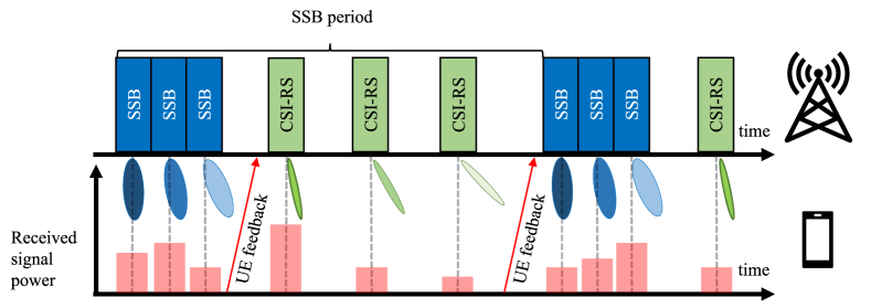
Figure 1: Beam sweeping-based beam alignment framework in 5G. The BS transmits beamformed SSB and CSI-RS. The UE measures and reports the quality of the RS. The BS selects a beam for future data or control transmission.

Hierarchical beam searches have been proposed to reduce the beam sweeping complexity [6],[7]. The BS and the UE, equipped with multiple-tier codebooks, sweep wider beams first and iteratively thin the search space for the best narrow beam. Since mmWave systems often employ analog or hybrid BF, the hardware constraints need to be considered when designing the wide beams in these hierarchical codebooks. Different hierarchical codebook design techniques have been proposed in recent works such as [8] and [9]. While the hierarchical search reduces the number of beams swept compared to an exhaustive one, the search procedure needs to be repeated for each UE, marginalizing the gain for multiple UEs. They are also more susceptible to search errors caused by noise in received signal and imperfect wide-beam patterns. The hierarchical search method proposed in [9] uses wide beams with multiple mainlobes to reduce the beam sweeping overhead for multiple UEs. However, the intermediate-layer beams need to be dynamically generated based on measurements of upper-layer beams, which lacks standardization support from 5G and also significantly increases the size of the effective hierarchical codebook.

In addition to the beam sweeping-based approaches, beam alignment methods that utilize context information has been explored. In [10],[11] and [12], the location information of UEs are used to reduce the beam search space. Beam alignment methods that utilizes sub-6 GHz measurements are proposed in [13], [14] and [15]. In [16], omni-directionally received sounding signals are used to predict the optimal beam. A beam alignment method assisted by radar measurements is proposed in [17]. However, such context information can be hard to obtain since mmWave devices need to be equipped with the required additional sensors. The feedback of such context information also incurs additional overhead and sometimes requires a more robust sub-6 GHz link between the BS and the UE.

ML solutions have been explored for the beam alignment problem. The pattern extraction and function approximation powers of ML models make them particularly suitable for processing a wide range of context information, such as location [11], sub-6 GHz channels [14] and omni-directional sounding signals [16]. A joint BF, power control and interference coordination method using reinforcement learning (RL) is proposed in [18]. A beam alignment method that uses CS to leverage channel sparsity is proposed in [19]. In [20], a deep learning architecture is used to learn CS matrices and predict the best beams.

Compared to the beam sweeping-based approaches, beam alignment solutions that rely on context information often require an additional cell search procedure to discover unconnected new UE regardless of whether traditional ML or deep learning techniques are used. The feedback of additional context information requires the UE to be connected to the network through mmWave links or sub-6 GHz side links, which can be problematic during IA. Furthermore, solutions that do not adopt beam sweeping are not compatible with the beam alignment framework in 5G. Significant modifications to the 5G standard is required to accommodate these approaches.

The NN architecture proposed in this work consists of a complex layer which represents the analog beam codebook and an MLP which acts as the beam selector. The complex-NN layer used in this work was first proposed in [21] for computer vision and audio-related tasks. A similar complex fully-connected layer is used in [22], where the authors optimize beam patterns for particular environments and hardware imperfections. This work focuses on finding an optimal beam from a large predefined narrow-beam codebook and differs from [22] which focuses on direct codebook learning.

In [23], a beam alignment method that trains a NN to predict optimal beams using UL measurements from a sparse probing codebook is proposed. However, the probing codebooks used in [23] are predetermined undersampled DFT codebooks with evenly spaced narrow beams, whereas the probing codebook in our proposed method are site-specific and learned using a complex-valued NN module. The NN in [23] requires knowledge of the complex received signals, whereas our proposed method only need the received power. We demonstrate in Section V-F that our learned probing codebooks are much more effective at capturing characteristics of the environment and providing useful information to the beam predictor.

I-B Contributions

In this work, we propose a beam alignment method that uses the beam sweeping measurements of a probing codebook to predict the optimal narrow beam. The proposed method is based on beam sweeping and does not require any additional context information, which is compatible with the beam alignment framework in 5G. By jointly training the probing codebook and the beam predictor using a NN in an end-to-end fashion, the probing codebook is able to learn particular characteristics of the propagation environment and optimize its beam patterns accordingly. Some key features of the proposed method are summarized as follows.

Trainable site-specific probing codebook: A complex-NN module is used to parameterize the probing codebook during training so that the BF weights can be extracted and implemented using actual RF chains during deployment. The probing codebook is able to learn particular characteristics of the propagation environment and optimize its beams to capture the channel information effectively. The proposed architecture can be adopted by BS in various deployment scenarios with arbitrary array geometry.

Compatibility with 5G framework: The proposed method can be directly adopted without modifications to the 5G standard. It does not require the collection and feedback of hard-to-obtain context information such as UE location or out-of-band information, which needs additional standardization support. Instead, the proposed method uses beam sweeping measurements of a probing codebook, which is exactly compatible with the beam sweeping-based framework currently adopted in 5G. The probing beams can be transmitted using SSB, which can also be used for cell discovery and IA.

High beam alignment accuracy and SNR: We demonstrate using multiple realistic ray-tracing datasets that the proposed method can achieve high beam alignment accuracy and SNR, beating the hierarchical beam search baselines. For instance, the proposed method can achieve a beam alignment accuracy of over 90% and can outperform even the exhaustive search in terms of the average SNR.

Reduced beam sweeping overhead: The proposed method has lower beam sweeping overhead compared to exhaustive and hierarchical beam searches, especially when considering beam alignment for multiple UE. For instance, when considering simultaneous beam alignment for 10 UE, the proposed method is about 3$\times$ faster compared to exhaustive and hierarchical beam searches.

Applicable to a wide range of propagation scenarios: Multiple accurate ray-tracing datasets modelling a wide range of propagation environments are used to evaluate the performance of the proposed method. The proposed beam alignment approach consistently achieves high accuracy and SNR in indoor and outdoor environments, for LOS and NLOS UE, and with 28 GHz and 60 GHz carrier frequencies.

The rest of this article is organized as follows. The system model is described in Section II. The proposed beam alignment approach, the appropriate metrics and the baselines of comparison are explained in Section III. The datasets used are described in Section IV. The simulation results are presented in Section V. Finally, the conclusion and final remarks are provided in Section VI.

II System Model

A DL MISO system is considered, where each BS has an antenna array of $N_{t}$ elements and each UE has a single antenna. While UE typically have antenna arrays also, we consider a MISO scenario where beam alignment is only performed on the BS side for simplicity. The MISO model is also applicable to the mMTC use case of 5G, where the each sensor would likely use a single antenna and an isotropic beam pattern. The extension to receive beam alignment on the UE side is left to future work. A ray-based narrowband block-fading mmWave channel model with $N_{p}$ paths is considered [24]:

$$\mathbf{h}=\sum_{l=1}^{N_{p}}\alpha_{l}\mathbf{a}(\phi_{l}^{D},\theta_{l}^{D}).$$ (1)

For each path $l$, its complex gain is $\alpha_{l}$, the azimuth and elevation angles of departure are $\phi_{l}^{D}$ and $\theta_{l}^{D}$, and the array steering vector at these angles is denoted by $\mathbf{a}(\phi_{l}^{D},\theta_{l}^{D})$. For a ULA with $N_{t}$ antenna elements on the $y$-axis, its beam steering is limited to the azimuth domain and its steering vector can be written as

$$\mathbf{a_{ULA}}(\phi_{l})=\frac{1}{\sqrt{N_{t}}}\begin{bmatrix}1&e^{j\frac{2\pi}{\lambda}d\sin\phi_{l}}&\cdots&e^{j(N_{t}-1)\frac{2\pi}{\lambda}d\sin\phi_{l}}\end{bmatrix}^{T},$$ (2)

where $\lambda$ is the carrier wavelength and d is the antenna spacing [25]. While a ULA is considered instead of a planar array for simplicity, the proposed beam alignment approach is array-geometry agnostic and can be applied to arrays of arbitrary geometry, as we will explain in Section III-A1.

Due to the cost and complexity of fully digital BF at mmWave frequencies, each BS is assumed to perform analog-only or hybrid BF. For the purpose of beam alignment, only the RF domain processing is considered. For a BS-UE pair, the BS is assumed to employ a single RF chain to which all antenna elements are connected. Analog BF is assumed to be implemented using phase shifters connected to each antenna element. The BF vector can be written as

$$\mathbf{v}=\frac{1}{\sqrt{N_{t}}}\begin{bmatrix}e^{j\theta_{1}}&e^{j\theta_{2}}&\cdots&e^{j\theta_{N_{t}}}\end{bmatrix}^{T},$$ (3)

where $\mathbf{v}$ satisfies the power constraint and each element of $\mathbf{v}$ satisfies the constant modulus constraint.

In the DL, the BS transmits a symbol $s\in\mathbb{C}$ satisfying average power constraint $\mathbb{E}[|s|^{2}]=1$ to the UE using a BF vector $\mathbf{v}$. The received signal at the UE can be written as

$$y=\sqrt{P_{T}}\mathbf{h}^{H}\mathbf{v}s+n,$$ (4)

where $P_{T}$ is the transmit power, $\mathbf{h}\in\mathbbm{C}^{N_{t}\times 1}$ is the channel vector and $n$ is the complex additive noise with noise power $\sigma_{n}^{2}$.

The SNR for a UE with channel $\mathbf{h}$ and using a BF vector $\mathbf{v}$ can be written as

$$\text{SNR}=\frac{P_{T}|\mathbf{h}^{H}\mathbf{v}|^{2}}{\sigma_{n}^{2}}.$$ (5)

The BS has a codebook $\mathbf{V}\in\mathbbm{C}^{N_{t}\times N_{\mathbf{V}}}$ of predefined narrow analog beams that are used for the data or the control channel, where each column of $\mathbf{V}$ represents the BF weights of a beam. The size of the narrow-beam codebook $N_{\mathbf{V}}$ is assumed to be large since $\mathbf{V}$ needs to cover the entire angular space. For a BS and a UE, the optimal narrow beam index is the one that achieves the maximum SNR:

$$i_{\mathbf{v}}^{*}=\mathop{\rm arg\,max}_{i\in\left\{1,2,\cdots,N_{\mathbf{V}}\right\}}\left(\frac{|\mathbf{h}^{H}\mathbf{v}_{i}|^{2}P_{T}}{\sigma_{n}^{2}}\right)=\mathop{\rm arg\,max}_{i\in\left\{1,2,\cdots,N_{\mathbf{V}}\right\}}(|\mathbf{h}^{H}\mathbf{v}_{i}|^{2}),$$ (6)

where $\mathbf{v}_{i}$ is the $i$th beam, i.e., the $i$th column of $\mathbf{V}$.

III The Proposed Method, Metrics and Baselines

We propose a beam alignment method that is compatible with the beam sweeping-based framework in 5G so that it can serve to achieve both beam alignment for connected UE and IA for unconnected UE using only beam sweeping measurements. With the proposed method, the BS first sweeps a small probing codebook to gather information about the channel then selects candidate narrow beams based on the probing-codebook measurements. In addition to the size-$N_{\mathbf{V}}$ narrow-beam codebook $\mathbf{V}\in\mathbbm{C}^{N_{t}\times N_{\mathbf{V}}}$ that is used for the data or the control channel, the BS also has a probing codebook $\mathbf{W}\in\mathbbm{C}^{N_{t}\times N_{\mathbf{W}}}$ with $N_{\mathbf{W}}$ beams. The size of the probing codebook $N_{\mathbf{W}}$ is much smaller than $N_{\mathbf{V}}$. The BS first sweeps its probing codebook $\mathbf{W}$. All UE connected to the BS measure and report the received power of the probing signals. The beam sweeping, measurement and reporting is assumed to be completed within the coherence time during which the channel remains the same. The reported beam sweeping results for each UE $u$ can be written as

$$\mathbf{x} =\begin{bmatrix}|y_{1}|^{2}&\cdots&|y_{N_{\mathbf{W}}}|^{2}\end{bmatrix}^{T},$$ (7)

where $y_{i}=\sqrt{P_{T}}\mathbf{h}^{H}\mathbf{w}_{i}s+n_{i}$ is the received signal using the $i$th probing beam (the $i$th column of $\mathbf{W}$). Given the reported power of received probing signals $\mathbf{x}$ of a UE, the BS then predicts the narrow beam index $i_{\mathbf{v}}\in\left\{1,2,\cdots,N_{\mathbf{V}}\right\}$ using a function $f:\mathbf{x}\rightarrow i_{\mathbf{v}}$. Overall, this problem can be formulated as

$$\begin{array}[]{rrclcl}\displaystyle\max_{\mathbf{W},f}&\lx@intercol{\mathop{\mathbb{E}}_{\mathbf{h}\in\mathcal{H}}}[|\mathbf{h}^{H}\mathbf{v}_{i_{\mathbf{v}}}|^{2}]\hfil\lx@intercol\\ \textrm{s.t.}&i_{\mathbf{v}}&=&f(\mathbf{x})\\ &|\mathbf{[W]}_{i,j}|&=&\frac{1}{\sqrt{N_{t}}},\forall i=1,\cdots,N_{t},\forall j=1,\cdots,N_{\mathbf{W}}.\\ \end{array}$$ (8)

The optimization problem in (8) is non-convex and difficult to solve due to the constant-modulus constraint of the probing BF weights and the unknown function $f$. The proposed method is analogous to a hierarchical beam search with 2 tiers. The probing codebook is similar to the wide-beam codebook in a hierarchical search in that they both provide rough information about the channel. Unlike the hierarchical search, the probing codebook consists of beam patterns adapted to the environment, which are not limited to wide beams. In a hierarchical method, the narrow-beam selection function $f$ picks the best child beam of the best wide beam, which incurs another round of beam measurement and report. In the proposed method, the narrow-beam selection function $f$ predicts good narrow beams by intelligently utilizing measurements of all probing beams instead of using a simple heuristic, e.g., picking the narrow beams pointing to the directions of the probing beam with the best measurement.

III-A The proposed NN architecture

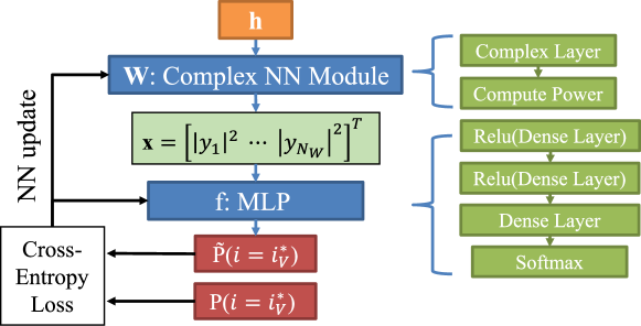
Figure 2: The architecture of the proposed NN, including the probing codebook $\mathbf{W}$ and the beam selection function $f$.

The probing codebook $\mathbf{W}$ needs to be designed so that its beam sweeping measurements provide useful information regarding which narrow beam in $\mathbf{V}$ to select. A good probing codebook is site-specific and should capture particular characteristics of the propagation environment. The beam selection function $f$ is also optimized for that particular BS and needs to be designed so that it picks narrow beams from $\mathbf{V}$ which tend to maximize the average SNR. Since the probing codebook $\mathbf{W}$ and the beam selection function $f$ are interdependent, they are parameterized with different NN modules – a complex-NN module and a MLP classifier – and jointly trained in an end-to-end fashion. The overall architecture is illustrated in Fig. 2.

III-A1 The trainable probing codebook

Beam sweeping using the probing codebook is modeled with a complex-NN module that computes the complex received BF signals and their power. The input to this NN module is the channel vector $\mathbf{h}$. The complex layer in the complex-NN module implements the complex arithmetic of analog BF using real arithmetic. When parameterizing a $N_{\mathbf{W}}$-beam codebook, the trainable weights of the complex layer are elements of $\Theta\in\mathbbm{R}^{N_{t}\times N_{\mathbf{W}}}$, which are the phase shift values applied to each antenna element. The complex BF weights $\mathbf{W}\in\mathbbm{C}^{N_{t}\times N_{\mathbf{W}}}$ can then be computed as

$$\mathbf{W}=\frac{1}{\sqrt{N_{t}}}(\cos{\Theta}+j\cdot\sin{\Theta}).$$ (9)

The complex matrix multiplication

$$\mathbf{z}=\mathbf{W}^{H}\mathbf{h}$$ (10)

can be expressed as a real matrix multiplication

$$\begin{bmatrix}\mathbf{z}^{real}\\ \mathbf{z}^{imag}\end{bmatrix}=\begin{bmatrix}\mathbf{W}^{real}&-\mathbf{W}^{imag}\\ \mathbf{W}^{imag}&\mathbf{W}^{real}\end{bmatrix}^{T}\begin{bmatrix}\mathbf{h}^{real}\\ \mathbf{h}^{imag}\end{bmatrix},$$ (11)

where $\mathbf{h}\in\mathbbm{C}^{N_{t}\times 1}$ is the channel vector, $\mathbf{z}\in\mathbbm{C}^{N_{\mathbf{W}}\times 1}$ is the BF output, and we express $\mathbf{z},\mathbf{W}$ and $\mathbf{h}$ in terms of their real and imaginary parts. The BF signal power can then be computed as

$$|\mathbf{z}|^{2}=\left[(\mathbf{z}_{1}^{real})^{2}+(\mathbf{z}_{1}^{imag})^{2},\cdots,(\mathbf{z}_{N_{\mathbf{W}}}^{real})^{2}+(\mathbf{z}_{N_{\mathbf{W}}}^{imag})^{2}\right]^{T}.$$ (12)

While $|\mathbf{z}|^{2}$ is not complex differentiable with respect to $\mathbf{z}$, backpropagation can be enabled by treating the real and imaginary parts of $\mathbf{z}$ independently and compute $\frac{\partial|\mathbf{z}|^{2}}{\partial\mathbf{z}^{real}}$ and $\frac{\partial|\mathbf{z}|^{2}}{\partial\mathbf{z}^{imag}}$. The phase-shift values $\Theta$ can then be updated using the chain rule and backpropagation. Since only the dimension of $\Theta$ needs to be specified when initializing the NN, the complex-NN module only needs to know the number of antenna elements and not the exact array geometry. The array-geometry information is embedded in the input channel vectors so that the complex-NN module can automatically learn the optimal phase-shift values to apply at each antenna element. This allows the architecture to be flexibly adopted by BS with different antenna arrays.

The complex-NN module computes the received signal power in (7). Since updates are made to the phase-shift values $\Theta$ during training, this architecture enforces the constant-modulus constraint of phase-shifter-only analog BF. Note that $\Theta$ can be extracted from the NN module at any time and be implemented as an analog codebook. After training, the complex-NN module can be discarded so that (7) can be computed using an actual RF chain and with an analog BF codebook derived from $\Theta$.

III-A2 The MLP beam selection function

The beam selection function $f$ is modeled using an MLP classifier, which is a feedforward fully connected NN with non-linear activation functions. The input to the MLP is the power of the complex received signals of all beams in $\mathbf{W}$, which is calculated using the complex-NN module during training or through beam sweeping during deployment. The MLP consists of several hidden layers before the output layer to increase its approximation power. The output of an MLP with 1 hidden layer can be written as

$$g(\mathbf{x})=b_{1}+A_{1}\sigma(b_{0}+A_{0}\mathbf{x}),$$ (13)

where the input feature vector is $\mathbf{x}$, the output vector is $g(\mathbf{x})$, the biases and weights of the hidden layer are $b_{0}$ and $A_{0}$, the biases and weights of the output layer are $b_{1}$ and $A_{1}$, and the non-linear activation function of the hidden layer is $\sigma$. The biases and weights models a trainable affine transformation, while the non-linear activation function allows the MLP to approximate a wide range of non-linear functions. The biases and weights of the NN can be updated through backpropagation to optimize some given objective function. One obvious way to optimize $f$ is to design it to predict the optimal narrow beam $\mathbf{v}^{*}$ which achieves the highest SNR with the current channel. Hence, the final softmax layer of the MLP outputs the predicted posterior probability distribution of each narrow beam in $\mathbf{V}$ being the optimal beam. The MLP is a powerful function approximator and can produce good estimates of posterior class probabilities. The BS can select the narrow beam with the highest predicted posterior probability. To increase the beam alignment robustness, the BS can also use the output of the MLP to reduce the search space and sweep the top-$k$ narrow beams with the highest predicted posterior probabilities.

The complex-NN architecture can be used to optimize a wide range of objective functions since it essentially implements analog BF while allowing gradient descent updates that respect the phase-shifter-only constraints. For instance, it is used to directly minimize the the mean squared error (MSE) between the gain of the strongest beam in the codebook and the equal gain combining (EGC) gain in [22]. It is also shown to be robust against hardware impairment [22]. In order to select an optimal beam from a given narrow-beam codebook, the probing codebook should provide useful information to the beam selection function based on the entire environment. Hence the MLP beam selection function is stacked after the complex-NN module and the entire NN is trained in an end-to-end fashion instead of directly optimizing the BF gain of the probing beams. The cross-entropy between the predicted optimal-beam distribution and the true optimal-beam distribution is used as the loss function. The partial derivative of the loss function with respect to the MLP biases and weights as well as $\Theta$ in the complex-NN module can be computed so that the MLP and the complex-NN module can be updated during training. The probing codebook is optimized implicitly to assist the downstream beam selection function. Interestingly, it still learns to capture particular characteristics of the propagation environment, as will be discussed in Section V-C.

III-B Practicality of the proposed method in 5G

The proposed beam alignment method requires an offline training phase and a deployment phase. During the training phase, the BS optimizes the probing codebook and the beam selection function by learning from training data and updating the NN. The training data consists of the channel vectors for a BS and its potential UE. Operators can obtain the channel vectors through ray-tracing simulations of the site prior to deployment. Alternatively, or for further refinement of the probing codebook, the BS can begin with a default codebook, and then gradually develop a site-specific probing codebook through interaction with its UE. In a typical TDD scenario, the BS can directly estimate the UL channel by receiving the SRS transmitted by UE and assume the DL channel is same as the estimated UL channel. If the DL and UL channel reciprocity does not exist, the UE can estimate the DL channel by receiving the SSB and CSI-RS transmitted by the BS and then feed back the estimated channel.

While the probing codebook is parameterized using a NN during training, the complex-NN module can be discarded in the deployment phase. As illustrated in Fig. 3, the BF weights of the probing codebook can be extracted from the complex-NN module and implemented as an analog beam codebook at the BS after training. During the deployment phase, the BS periodically sweeps the learned probing codebook by transmitting a sequence of SSB using different probing beams. Each UE measures all the SSB and reports the received signal power to the BS. The received signal power vector $\mathbf{x}$ is fed into the MLP beam predictor at the BS, which then selects the optimal narrow beam or a few candidate beams to try according to the predicted posterior probability distribution. If the BS chooses to search the top-$k$ predicted narrow beams for additional robustness, it can do so by sweeping those beams using the aperiodic CSI-RS, which can be independently configured for each UE. The proposed beam alignment method is adapted to characteristics of the propagation environment such as the distribution of UE and the location of the scatterers. If the environment changes, the probing codebook as well as the MLP beam predictor need to retrained. The NN modules can be trained from scratch, or be initialized with the existing probing codebook and MLP weights and be refined using data from the new environment. The retraining can be triggered if the beam alignment performance is below a threshold. Since such macroscopic characteristics of the environment are expected to evolve slowly, the retraining should occur infrequently.

The proposed beam alignment method essentially consists of periodic beam sweeping by the BS and beam measurement and reporting by the UE during the deployment phase. This beam sweeping, measurement and reporting process precisely fits into the beam sweeping-based framework currently adopted in 5G, as discussed in Section I-A. Instead of sweeping a general codebook using SSB to cover the entire angular space, the proposed method sweeps a site-specific probing codebook that learns to strategically place beams in directions that can effectively capture characteristics of the environment and provide useful information to the downstream beam selector. Since the learned probing codebook replaces traditional full-coverage codebooks, its beams can be transmitted using “always-on” SSB and thus can also be used by unconnected UE for cell discovery and IA. Instead of selecting the narrow beam with the highest reported power and ignoring the measurement of the rest of the codebook, the proposed method predicts good candidate beams using a NN that intelligently utilizes the measurement of all probing beams. This is also supported in 5G since the BS can request additional beam reports from UE to obtain measurements of all probing beams. Overall, the proposed method can be directly adopted in 5G and does not require any modification to the existing 5G standard.

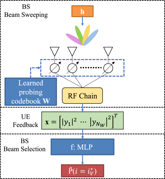
Figure 3: Proposed beam alignment architecture during the deployment phase.

III-C Baselines and Metrics

The proposed beam alignment method selects the optimal narrow beam based on measurements of a probing codebook. It is analogous to a hierarchical beam search where the optimal narrow child beam is determined based on measurements of wider parent beams. In a traditional hierarchical beam search, the BS needs to sweep all child beams of the best parent beam at each layer of the codebook. The parent beam needs to have a wider beam width and should contain the coverage areas of its child narrower beams. Four baselines of comparison are considered, including 2 hierarchical beam searches, an exhaustive beam search and a genie. In all baselines, the BS has the same narrow-beam codebook $\mathbf{V}\in\mathbbm{C}^{N_{t}\times N_{\mathbf{V}}}$ with $N_{\mathbf{V}}$ beams from which it needs to select a beam for the data or control channel. When comparing the performance of different beam alignment methods, the beam alignment accuracy and the SNR are two key metrics. The beam alignment accuracy is the probability or relative frequency that the BS selects the optimal narrow beam from the codebook $\mathbf{V}$. The SNR is calculated as in (5).

2-Tier Hierarchical Beam Search The 2-tier hierarchical beam search uses a wide-beam codebook with $N_{\mathbf{W}}$ beams and a narrow-beam codebook with $N_{\mathbf{V}}\gg N_{\mathbf{W}}$ beams, both covering the same angular space. Each narrow beam is the child beam of one of the wide beams. The coverage area of each wide beam contains the coverage areas of all of its children beams. The BS first sweeps the $N_{\mathbf{W}}$ wide beams then sweeps the children beams of the best wide beam. The final selected beam is the best child beam of the best wide beam. The wide-beam codebook is analogous to the proposed probing codebook in that they both provide rough information about the channel for beam selection.

Binary Hierarchical Beam Search The binary hierarchical beam search is a generalized version of the 2-tier beam search. It performs a binary tree search on the narrow beam codebook $\mathbf{V}$. Starting with a search space equal to the entire angular space, the BS repeatedly splits the search space into two partitions and sweeps two wide beams each covering one of the partitions until reaching one of the narrow beams in the final codebook $\mathbf{V}$. With $N_{\mathbf{V}}$ narrow beams, each beam search consists of $\log_{2}N_{\mathbf{V}}$ layers. With more hierarchical search layers, the binary beam search is more susceptible to search errors compared to the 2-tier search. If a sub-optimal wide beam is chosen in any of the upper layers due to noise or imperfect wide-beam patterns, the error will propagate forward and affect the selected narrow beam in $\mathbf{V}$.

Exhaustive Beam Search The BS exhaustively sweeps the narrow beam codebook $\mathbf{V}$ with $N_{\mathbf{V}}$ beams and selects the beam with the highest received power. Compared to a hierarchical beam search, the exhaustive search directly measures the narrow-beam codebook instead of some wide-beam intermediate codebooks. The best beam in the narrow-beam codebook has larger directionality gain compared to the wide beams used in the hierarchical methods. As a result, the exhaustive search is less susceptible to noise in the beam measurements.

Genie (Upper Bound) The BS has knowledge of the true BF gain of each narrow beam in the codebook $\mathbf{V}$ and always selects the best beam. While the hierarchical searches and the exhaustive search are all susceptible to search errors caused by noise in the received BF signal, the genie method is not. If the receive noise power is zero, the genie is equivalent to the exhaustive beam search; else it is strictly better than exhaustive search. Given a narrow-beam codebook $\mathbf{V}$, the genie method achieves a perfect beam alignment accuracy of 100% and provides a performance upper bound.

The hierarchical beam search approaches require wide beams that contain the coverage area of their children narrower beams. Multiple works have studied hierarchical codebook designs. Synthesizing wide beams often requires multiple RF chains or antenna activation, such as in [26], [27] and [8]. Since a single RF chain and analog BF only is assumed in this work, the AMCF algorithm proposed in [9] is used to generate the wide beams in the hierarchical codebooks.

IV Dataset

Realistic and accurate data is essential to learning good NN models. Ray tracing is able to achieve high accuracy and maintain spatial consistency when modeling mmWave channels. A state-of-the-art commercial-grade ray-tracing software called Wireless InSite [28] is used to generate the channel data. The ray-tracing software simulates rays emitting from the transmitter at all directions in the angular space and computes their interaction with the environment along their paths before reaching the receiver, including scattering, reflection and blockage. An environment needs to be constructed in the ray-tracing software, specifying the terrain, the scatterers and their dielectric properties.

Four different ray-tracing scenarios are considered to capture a wide range of propagation environments for mmWave: a dense urban outdoor area, an urban street, an indoor conference room with hallways and an urban street with severe blockage and reflections. The ray-tracing scenarios include both LOS and NLOS UE and cover two different mmWave carrier frequencies: 28 GHz and 60 GHz. The ray-tracing simulation parameters are summarized in Table I.

Rosslyn Experiment The Rosslyn dataset captures an outdoor dense urban environment located in downtown Rosslyn, Virginia, USA. It was created with our own experiments and was published in [11]. A 3-D render of the environment is shown in Fig. 4. The Rosslyn environment has multiple buildings surrounding an intersection. A BS is placed at the center of the intersection, elevated by 10 meters above the ground. A total of 73,884 UE positions are placed uniformly 0.35 meter apart and 2 meters above the terrain surface. The entire simulated area is around 90 meters $\times$ 90 meters. The Rosslyn environment consists of mostly LOS UE and uses a carrier frequency of 28 GHz.

DeepMIMO O1_28 Experiment The DeepMIMO O1_28 dataset captures an outdoor street environment and is available in the public DeepMIMO dataset [29]. A portion of the original dataset corresponding to BS #3 and UE in row #800 to row #1200 is selected. The environment consists of a street with buildings on both sides. The BS is placed on one side of the street with an elevation of 6 meters. A total of 72,581 UE positions are placed uniformly on the street 20 centimeters apart. The environment consists of mostly LOS UE and uses a carrier frequency of 28 GHz.

DeepMIMO I3 Experiment The DeepMIMO I3 dataset models an indoor conference room and its hallways and is available in the public DeepMIMO dataset [29]. A 3-D view of the environment is shown in Fig. 5. A BS is placed 2 meters high on the wall inside the conference room. A total of 118,959 UE positions are placed inside two grids: one LOS grid inside the conference room and one NLOS grid in the hallway. The carrier frequency is 60 GHz.

DeepMIMO O1_28B Experiment The DeepMIMO O1_28B outdoor street environment is similar to the O1_28 scenario [29] but with severe blockage and reflections. A 2-D illustration of the environment is shown in Fig. 6. A 24-meter-wide metal screen is placed in front of the BS and two reflectors are placed on both sides. A total of 497,931 UE positions are placed uniformly on the street 20 centimeters apart. This environment includes both LOS and NLOS UE and uses a carrier frequency of 28 GHz.

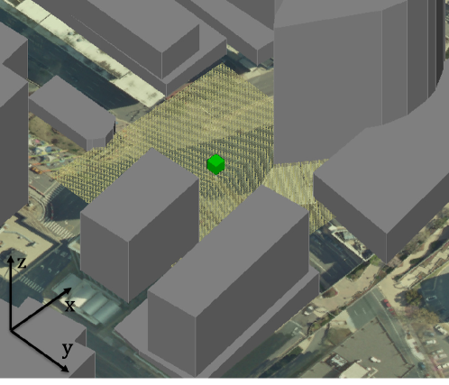
Figure 4: 3-D view of the Rosslyn environment. The green block represents the BS. Points on the yellow grid represent the UEs.

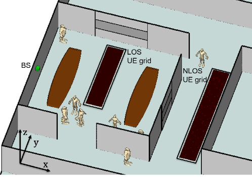
Figure 5: 3-D view of the DeepMIMO I3 environment. Adapted: [30]

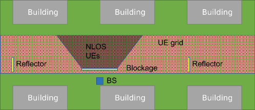
Figure 6: 2-D illustration of the DeepMIMO O1_28B environment. Dimensions are not to scale.

V Evaluation

Accurate ray-tracing channel data is used in our experiments as described in Section IV. In all experiments, 60% of the data is used for training, 20% of the data is used for validation and the remaining 20% is used for testing. The training dataset is used to optimize the NN weights. The hyperparameters of the NN are tuned by performing a grid search over a set of predefined values and comparing their performance on the validation set. The test set is used to evaluate the final performance of each beam alignment method. The MLP module in the proposed NN architecture has 2 hidden layers with rectified linear unit (ReLU) activation. The NN is trained for 200 epochs using the Adam optimizer [31]. The training and validation loss after each training epoch is examined to ensure that the NN has converged. A complex AWGN is assumed. The noise power in the received BF signal in (4) is -81 dBm unless otherwise specified. The simulation parameters are summarized in Table I. To make training more stable and efficient, the channel vectors are normalized by the maximum magnitude of the elements in the dataset: $\max_{\mathbf{h}\in\mathcal{H}}|\mathbf{h}_{i,j}|$. Similar normalization techniques are adopted in [16] and [22]. The noise is also scaled appropriately according to the normalization factor. Since the normalization factor is a predetermined constant that only depends on the underlying environment, it should not affect the practicality of the proposed method. The final narrow beam codebook $\mathbf{V}$ is a 128-beam DFT codebook.

TABLE I: Simulation Parameters

BS Antenna	$64\times 1$ ULA
UE Antenna	Single
Narrow beam codebook size $N_{\mathbf{V}}$	128
Carrier Frequency	Rosslyn, DeepMIMO O1_28, O1_28B: 28 GHz DeepMIMO I3: 60 GHz
Bandwidth ($B$)	100 MHz
Transmit Power ($P_{T}$)	Rosslyn, DeepMIMO O1_28, I3: 10 dBm DeepMIMO O1_28B: 20 dBm
Noise power spectral density (PSD)	-161 dBm / Hz
Number of Rays	25

V-A Can the proposed beam alignment method achieve good accuracy?

The accuracy of the proposed method and the baselines with increasing probing codebook size is shown in Fig. 7. The genie always has a perfect accuracy of 1 and is not shown in the figure. The accuracy of the proposed method increases as the number of probing beams increases, which is expected since a larger probing codebook allows the BS to obtain more information about the channel for a UE. Among the traditional beam sweeping-based baselines, the exhaustive search performs the best and the binary search performs the worst. This is expected since a method with more layers in the hierarchical search structure is more vulnerable to noise in the received signal. Instead of directly choosing the predicted optimal beam, the accuracy of the proposed method can be improved significantly by searching a few additional candidate beams. In all 4 environments, the proposed method can achieve a beam alignment accuracy of at least 85% with just 14 probing beams and searching an additional $k$ = 3 narrow beams, outperforming both the binary and the 2-tier hierarchical beam search baselines. In the 2 LOS environments (Rosslyn and DeepMIMO O1_28), the proposed method can beat the binary beam search with 10 probing beams and $k$ = 3. With 16 probing beams, it can even outperform the exhaustive search by sweeping an additional $k$ = 3 narrow beams. In the 2 environments with NLOS UE (DeepMIMO I3 and O1_28B), traditional beam sweeping-based baselines perform considerably worse compared to in the LOS environments. The exhaustive search can only achieve an accuracy of around 80% compared to around 90% in the LOS environments. The hierarchical beam searches suffer from even worse accuracy degradation, with the 2-tier hierarchical beam search achieving accuracies of around 65% compared to around 80% in the LOS environments. Clearly, beam alignment for the NLOS UE is more challenging for traditional beam sweeping-based baselines. On the other hand, the proposed method shines in these environments with NLOS UE. With just 8 probing beams and $k$ = 3, it outperforms any beam sweeping-based baseline, including the exhaustive search. With 12 probing beams and $k$ = 3, the proposed method can achieve an accuracy of over 84% in the I3 environment and over 88% in the O1_28B environment. Overall, the proposed method can outperform the traditional beam sweeping-based baselines with a moderate probing codebook size, particularly in environments with NLOS UE which are usually challenging for beam alignment.

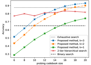
(a) Rosslyn

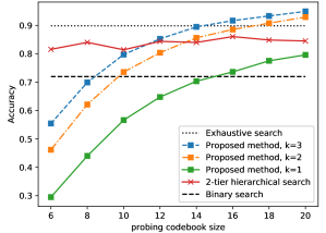
(b) DeepMIMO O1_28

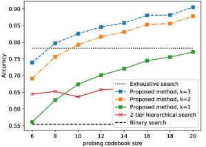
(c) DeepMIMO I3

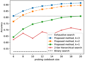
(d) DeepMIMO O1_28B

Figure 7: Beam alignment accuracy vs. probing codebook size.

V-B Can the proposed beam alignment method achieve good SNR?

The beam alignment accuracy considers the probability of finding the optimal narrow beam. With a large, oversampled codebook, adjacent narrow beams may have similar BF gains. As a result, operators may be more interested in the SNR achieved after beam alignment. The average SNR of the proposed method and the baselines with increasing probing codebook size is shown in Fig. 8. In the LOS environments (Rosslyn and DeepMIMO O1_28), the proposed method outperforms the binary beam search with just 10 probing beams and $k$ = 2 but is worse than both the exhaustive and the 2-tier hierarchical methods. It is able to match the 2-tier hierarchical baseline in terms of average SNR with 20 probing beams and $k$ = 3. The exhaustive search achieves close-to-optimal average SNR while its accuracy is just around 90%. Similar to the accuracy performance, the proposed method shines in the challenging NLOS environments in terms of average SNR. With just 8 probing beams and without additional narrow-beam sweeping, it outperforms both hierarchical search methods. With 12 probing beams and $k$ = 3, the proposed method can achieve similar if not better average SNR compared to the exhaustive search. Overall, with 12 probing beams and $k$ = 3, the gap in the average SNR of the proposed method from the genie upper bound is 3.73 dB in the Rosslyn environment, 2.86 dB in the DeepMIMO O1_28 environment, 1.36 dB in the I3 environment and 2.15 dB in the O1_28B environment.

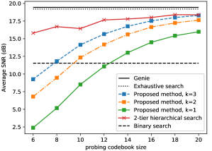
(a) Rosslyn

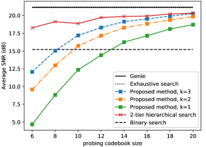
(b) DeepMIMO O1_28

(c) DeepMIMO I3

(d) DeepMIMO O1_28B

Figure 8: Average SNR vs. probing codebook size.

V-C Can the proposed NN learn meaningful probing codebooks?

The learned probing codebook should provide meaningful and helpful information to the downstream MLP beam predictor. In the proposed end-to-end training procedure, the complex-NN probing codebook and the MLP beam predictor are jointly trained. Intuitively, the complex-NN module should learn beam patterns that can effectively capture the characteristics of the underlying environment. The DeepMIMO O1_28 and O1_28B environments provide a good case study. Both environments feature similar topologies where a roadside BS serves UE located on the street. While all UE are LOS in the O1_28 environment, a significant portion of the UE are NLOS due to blockage by a metal screen placed in front of the BS in the O1_28B environment. In order to provide coverage to the NLOS UE, the BS in the O1_28B environment needs to steer beams towards the two reflectors on both sides of the street. The majority of the LOS UE are also distributed on both sides of the BS.

The learned probing codebook patterns in both environments is shown in Fig. 9. Firstly, the learned radiation patterns are similar with increasing probing codebook sizes $N_{\mathbf{W}}$ in either environment. Regardless of the codebook size, the probing codebook consistently learns to focus energy on specific areas. This indicates that the complex-NN module can consistently learn probing codebook patterns in a given environment. Unlike conventional DFT beams which have a single main lobe, the learned beams often have multiple main lobes. Such beam patterns can likely capture more information about the propagation environment given the small number of probing beams allowed. Furthermore, the learned probing codebooks are adapted to the particular characteristics of different environments. The learned beam patterns in the O1_28 environment are drastically different from those in O1_28B. In the O1_28B environment, the codebooks are optimized to focus energy in the angular regions close to $\pm 90^{\circ}$, corresponding to the positions of the LOS UE and the reflectors. In comparison, the codebooks learned in the O1_28 environment spread the energy much more evenly in the broadside direction, which is consistent with the even distribution of LOS UE in front of the BS in this environment. While the complex-NN module is not explicitly optimized to leverage spatial patterns of the environment, it can nevertheless consistently learn probing beams that captures particular characteristics of the environment.

(a) O1_28, $N_{\mathbf{W}}=6$

(b) O1_28, $N_{\mathbf{W}}=8$

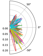
(c) O1_28, $N_{\mathbf{W}}=10$

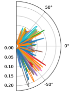
(d) O1_28, $N_{\mathbf{W}}=12$

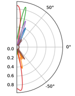
(e) O1_28B, $N_{\mathbf{W}}=6$

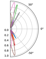
(f) O1_28B, $N_{\mathbf{W}}=8$

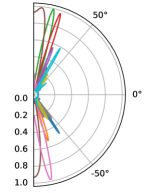
(g) O1_28B, $N_{\mathbf{W}}=10$

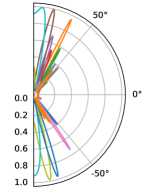
(h) O1_28B, $N_{\mathbf{W}}=12$

Figure 9: Learned beam patterns with different probing codebook sizes in the DeepMIMO O1_28 and O1_28B environments.

V-D Does the proposed method achieve lower beam sweeping complexity?

With the proposed beam alignment method, all UE can measure the probing beams simultaneously when the BS sweeps the probing codebook. If the BS choose to sweep the top-$k$ predicted beams, those beams may be different for each UE. Hence the beam sweeping complexity is $N_{\mathbf{W}}+K\cdot k_{\mathbbm{1}_{\{k>1\}}}$ for $K$ UE. Each UE needs to feedback the received signal power of the $N_{\mathbf{W}}$ probing beams. If the BS choose to sweep additional beams, each UE only needs to feedback the index of the best beam. With the 2-tier hierarchical beam search, the 1st-tier wide beams can be transmitted using SSB and be measured by all UE simultaneously, while different 2nd-tier children beams need to be swept for each UE. On average, the beam sweeping complexity is $N_{\mathbf{W}}+K\frac{N_{\mathbf{V}}}{N_{\mathbf{W}}}$ for $K$ UE. Each UE needs to feedback the index of the best beam in each tier. With the binary hierarchical beam search, the two first layer beams can be measured simultaneously by all UE while the subsequent beam sweeping needs to be done for each different UE. Hence the beam sweeping complexity is $2+2K\log_{2}\frac{N_{\mathbf{V}}}{2}$ for $K$ UE. Each UE needs to feedback the index of the best beam in each level of the binary search. With the exhaustive beam search, the $N_{\mathbf{V}}$ beams can be measured by all UEs simultaneously. The beam complexity is $N_{\mathbf{V}}$ regardless of the number of UE. Each UE needs to feedback the index of the best beam. A summary of the beam sweeping and feedback complexity of the proposed method and the baselines is shown in Table II.

TABLE II: Beam Sweeping Complexity for $K$ UEs

Beam alignment method	Beam sweeping complexity	Feedback complexity
Proposed method	$N_{\mathbf{W}}+K\cdot k_{\mathbbm{1}_{\{k>1\}}}$	$KN_{\mathbf{W}}$ received signal power + $K\cdot\mathbbm{1}_{\{k>1\}}$ beam indices
2-tier hierarchical search	$N_{\mathbf{W}}+K\frac{N_{\mathbf{V}}}{N_{\mathbf{W}}}$	$2K$ beam indices
Binary hierarchical search	$2+2K\log_{2}\frac{N_{\mathbf{V}}}{2}$	$K\log_{2}N_{\mathbf{V}}$ beam indices
Exhaustive search	$N_{\mathbf{V}}$	$K$ beam indices

A comparison of the beam sweeping complexity with 1,5,10 and 15 UE is shown in Fig.10. When considering a single UE, the proposed method has lower beam sweeping complexity compared to the exhaustive search and the 2-tier hierarchical beam search. With fewer than 11 probing beams, the proposed method also incurs lower beam sweeping complexity than the binary beam search does even when sweeping 2 or 3 additional beams. When considering simultaneous beam alignment for multiple UE such as 5, 10 and 15 UE, the beam sweeping complexity of the proposed method is lower than that of any baseline. In the 2 NLOS environments (DeepMIMO I3 and O1_28B), when considering simultaneous beam alignment for 10 UE, the proposed method with 12 probing beams and $k=3$ can achieve an average SNR similar to that of the exhaustive beam search, at least 3.65 dB better than that of the 2-tier hierarchical beam search and at least 7.71 dB better than that of the binary beam search, while incurring less than 35.4% of the beam sweeping complexity of any baseline. With 12 probing beams but without additional beam sweeping ($k=1$), the proposed method can still beat the hierarchical search baselines while reducing the beam sweeping complexity by 10$\times$.

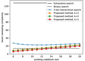
(a) 1 UE

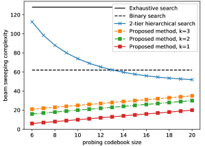
(b) 5 UEs

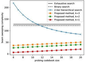
(c) 10 UEs

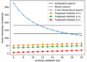
(d) 15 UEs

Figure 10: Beam sweeping complexity vs. probing codebook size.

V-E Is the proposed beam alignment method robust to noise?

The proposed beam alignment method, like any beam sweeping-based approach, relies on measurements of the received power of the BF signals. As a result, noise in the received BF signal may have significant impacts on the beam alignment performance. We compare the beam alignment accuracy at various noise levels to that when there is no noise. The accuracy degradation is defined as the absolute difference between the accuracy with no noise and the accuracy at a certain SNR level. The accuracy degradation at various SNR levels is shown in Fig. 11. In the LOS environments (Rosslyn and DeepMIMO O1_28), the accuracy degradation of all compared methods is minimal when the SNR is over 35 dB. When the SNR is between 5 dB and 25 dB, the exhaustive search experiences the least amount of accuracy drop. The proposed method with $k$ = 3 experiences similar levels of degradation compared to the hierarchical search baselines. In the NLOS environments (DeepMIMO I3 and O1_28B), the accuracy degradation is much more noticeable even at high SNR levels of over 35 dB. The proposed method also performs more favorably in terms of accuracy drop. With $k$ = 3, it experiences the least amount of accuracy degradation when the SNR is over 15 dB in the DeepMIMO I3 environment. In the O1_28B environment, the proposed method experiences less degradation than any other baseline at all SNR levels.

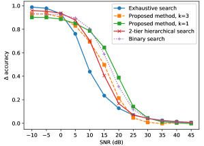
(a) Rosslyn

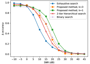
(b) DeepMIMO O1_28

(c) DeepMIMO I3

(d) DeepMIMO O1_28B

Figure 11: Beam alignment accuracy gap vs. SNR. The vertical axis represents the accuracy degradation from when there is no noise in the received signal. The horizontal axis represents the average SNR of the optimal narrow beams of all UEs.

V-F How does the learned probing codebook help the beam predictor?

The trainable probing codebook is an important part of the proposed bean alignment method and should be optimized to help the subsequent optimal-beam classification task. To verify this, the performance of the MLP classifier is evaluated while the trainable probing codebook is replaced with a predetermined probing codebook. Two predetermined probing codebooks are considered: a DFT codebook with $N_{\mathbf{W}}$ evenly-spaced narrow beams which is similar to the sparse codebook used in [23], and a wide-beam codebook whose $N_{\mathbf{W}}$ evenly-spaced wide beams are generated using the AMCF algorithm. The MLP is trained from scratch using the received signal power of each predetermined probing codebook. A beam alignment accuracy comparison of the learned probing codebook and the predetermined ones in all 4 environments is shown in Fig. 12. In all 4 environments, the learned probing codebook achieves significantly better beam alignment accuracy. By placing beams strategically according to the propagation environment instead of evenly in the angular space regardless of the environment, the learned probing codebook is much more effective at capturing channel characteristics, which greatly benefits the downstream classification task.

(a) Rosslyn

(b) DeepMIMO O1_28

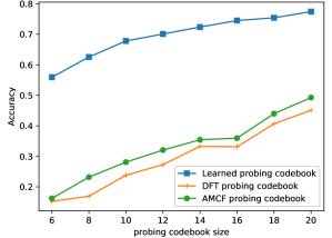
(c) DeepMIMO I3

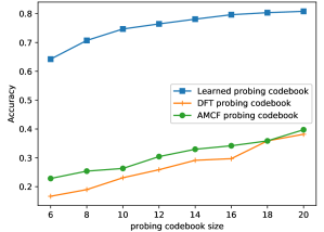
(d) DeepMIMO O1_28B

Figure 12: Accuracy vs. probing codebook size.

The probing codebook can also be viewed through the lens of data clustering and representation learning, which provides a further explanation of how the learned codebook help select the optimal beam. By performing beam sweeping using the probing codebook, the high-dimensional channel vector $\mathbf{h}\in\mathbbm{C}^{N_{t}\times 1}$ is transformed into a feature vector of received signal power values $\mathbf{x}\in\mathbbm{R}^{N_{\mathbf{W}}\times 1}$ lying in a lower-dimensional subspace determined by the probing codebook. If the transformed feature vectors with the same optimal narrow beam are assigned to the same cluster, a good probing codebook should intuitively make clusters corresponding to different narrow beams well separated so that the MLP can more easily predict the optimal beam. After beam sweeping using the probing codebook, channel realizations with the same optimal narrow beam should be close to each other in the transformed subspace, while those with different optimal narrow beams should be farther apart. This is similar to the representation learning problem in ML, which often seeks to learn low-dimensional representations of high-dimensional data that exhibits natural clustering according to the data labels [32]. One measure of the clustering quality is the silhouette coefficient [33]. For a dataset $\mathcal{D}$, its silhouette coefficient $S(\mathcal{D})\in[-1,1]$ is

$$S(\mathcal{D})=\mathop{\mathbb{E}}_{i\in\mathcal{D}}\Big{[}\frac{b(i)-a(i)}{\max\{a(i),b(i)\}}\Big{]},$$ (14)

where $a(i)$ is the mean intra-cluster distance of a data sample $i$ and $b(i)$ is its distance to the nearest cluster of which it is not a part of. A higher silhouette coefficient indicates better clustering and better separability of the data, which will likely make classifying the optimal beam easier. The silhouette coefficients of the received signal power vector $\mathbf{x}$ in all 4 environments are shown in Table III. Compared to the predefined AMCF and DFT probing codebooks, the learned codebook consistently achieves better silhouette coefficients regardless of the environment and the number of probing beams, thus explaining its superior beam alignment performance.

To further visualize the clustering effect of the probing codebooks, 2-D embeddings of the probing codebook measurements $\mathbf{x}$ are learned using the t-SNE algorithm. The t-SNE algorithm [34] is commonly used to learn low-dimensional embeddings of high-dimensional data while preserving its distribution in the high-dimensional space, so that similar data samples are more likely to be closer together and dissimilar ones are more likely to be farther apart in the embedding space. Two environments – Rosslyn and DeepMIMO O1_28 – are selected as case studies, and their t-SNE visualizations are shown in Fig. 13. With the AMCF and the DFT probing codebooks, the clusters have elongated and twisted shapes. With the learned codebook, the data samples within each cluster are more tightly packed. The learned probing codebook allows the channel realizations to form better-shaped clusters which will likely make the data easier to classify.

TABLE III: Silhouette Coefficients of Beam Sweeping Received Signal Power

Environment	Probing codebook	Probing codebook size
		6	8	10	12	14	16	18	20
Rosslyn	learned	-0.179	-0.144	-0.118	-0.099	-0.078	-0.071	-0.051	-0.035
	AMCF	-0.333	-0.266	-0.262	-0.242	-0.215	-0.196	-0.172	-0.160
	DFT	-0.376	-0.404	-0.320	-0.281	-0.231	-0.231	-0.189	-0.199
DeepMIMO O1_28	learned	-0.256	-0.231	-0.196	-0.173	-0.175	-0.151	-0.161	-0.119
	AMCF	-0.367	-0.337	-0.316	-0.290	-0.281	-0.283	-0.250	-0.238
	DFT	-0.426	-0.380	-0.353	-0.340	-0.329	-0.302	-0.272	-0.292
DeepMIMO I3	learned	-0.302	-0.255	-0.223	-0.218	-0.206	-0.191	-0.190	-0.177
	AMCF	-0.505	-0.477	-0.440	-0.406	-0.391	-0.390	-0.366	-0.349
	DFT	-0.503	-0.480	-0.416	-0.393	-0.385	-0.399	-0.361	-0.364
DeepMIMO O1_28B	learned	-0.597	-0.584	-0.588	-0.573	-0.573	-0.572	-0.571	-0.571
	AMCF	-0.623	-0.618	-0.616	-0.612	-0.608	-0.611	-0.604	-0.601
	DFT	-0.746	-0.742	-0.696	-0.683	-0.668	-0.662	-0.641	-0.634

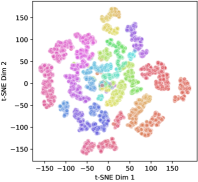
(a) Rosslyn, learned

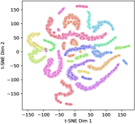
(b) Rosslyn, AMCF

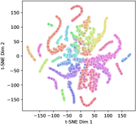
(c) Rosslyn, DFT

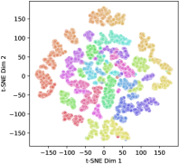
(d) DeepMIMO O1_28, learned

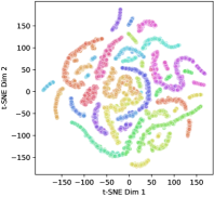
(e) DeepMIMO O1_28, AMCF

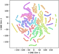
(f) DeepMIMO O1_28, DFT

Figure 13: t-SNE visualization of the received signal power of different probing codebooks with $N_{\mathbf{W}}=16$ beams.

VI Conclusion

We propose a mmWave beam alignment method that uses ML to predict the optimal narrow beam using measurements of a learned probing codebook. We design a NN architecture that optimizes the site-specific probing codebook so that it can capture particular characteristics of the propagation environment. After an offline training phase, operators can implement the learned probing codebook using an RF chain and use its beam sweeping results to select an optimal narrow beam or a few candidate beams to try, which is compatible with the beam alignment framework in 5G. The proposed method can outperform hierarchical beam search baselines and even the exhaustive beam search, particularly in challenging environments with NLOS UE, while significantly reducing the beam sweeping overhead. We also provide an explanation of why the learned probing codebook is beneficial to the beam alignment task through the lens of data clustering and representation learning. The proposed method uses channel information during its offline training phase. Future works may consider beam prediction without offline training or explicit channel knowledge. The complex-NN architecture may also be extended to consider hybrid BF. The extension to receive beam alignment on the UE side is another promising direction.

VII Acknowledgements

The authors thank V. Va, A. Ali and B.L. Ng from Samsung Research America for their valuable feedback and discussion.

References

- [1] Y. Heng, J. Mo, and J. G. Andrews, “Learning probing beams for fast mmWave beam alignment,” submitted to IEEE GLOBECOM 2021.
- [2] Study on supporting NR from 52.6 GHz to 71 GHz (Release 17), document 3GPP TR 38.808, Mar. 2021.
- [3] M. Giordani, M. Polese, A. Roy, D. Castor, and M. Zorzi, “A tutorial on beam management for 3GPP NR at mmWave frequencies,” IEEE Communications Surveys Tutorials, vol. 21, no. 1, pp. 173–196, Sep. 2019.
- [4] Y. R. Li, B. Gao, X. Zhang, and K. Huang, “Beam management in millimeter-Wave communications for 5G and beyond,” IEEE Access, vol. 8, pp. 13 282–13 293, Jan. 2020.
- [5] Y. Heng, J. G. Andrews, J. Mo, V. Va, A. Ali, B. L. Ng, and J. C. Zhang, “Six key challenges for beam management in 5.5G and 6G systems,” Submitted for publication, 2021.
- [6] V. Desai, L. Krzymien, P. Sartori, W. Xiao, A. Soong, and A. Alkhateeb, “Initial beamforming for mmWave communications,” in Proc. ASILOMAR, Nov. 2014, pp. 1926–1930.
- [7] M. Giordani, M. Mezzavilla, C. N. Barati, S. Rangan, and M. Zorzi, “Comparative analysis of initial access techniques in 5G mmWave cellular networks,” in Proc. Annu. Conf. Inf. Sci. Syst. (CISS), Mar. 2016, pp. 268–273.
- [8] Z. Xiao, T. He, P. Xia, and X.-G. Xia, “Hierarchical codebook design for beamforming training in millimeter-wave communication,” IEEE Trans. Wireless Commun., vol. 15, no. 5, pp. 3380–3392, May 2016.
- [9] C. Qi, K. Chen, O. A. Dobre, and G. Y. Li, “Hierarchical codebook-based multiuser beam training for millimeter wave massive MIMO,” IEEE Trans. Wireless Commun., vol. 19, no. 12, pp. 8142–8152, Sep. 2020.
- [10] Y. Wang, A. Klautau, M. Ribero, A. C. K. Soong, and R. W. Heath, “MmWave vehicular beam selection with situational awareness using machine learning,” IEEE Access, vol. 7, pp. 87 479–87 493, Jun. 2019.
- [11] Y. Heng and J. G. Andrews, “Machine learning-assisted beam alignment for mmWave systems,” IEEE Trans. Cogn. Commun. Netw., pp. 1–1, May 2021, early access.
- [12] V. Va, J. Choi, T. Shimizu, G. Bansal, and R. W. Heath, “Inverse multipath fingerprinting for millimeter wave V2I beam alignment,” IEEE Trans. Veh. Technol., vol. 67, no. 5, pp. 4042–4058, Dec. 2017.
- [13] A. Ali, N. González-Prelcic, and R. W. Heath, “Millimeter wave beam-selection using out-of-band spatial information,” IEEE Trans. Wireless Commun., vol. 17, no. 2, pp. 1038–1052, Feb. 2018.
- [14] M. Alrabeiah and A. Alkhateeb, “Deep learning for mmwave beam and blockage prediction using sub-6 GHz channels,” IEEE Trans. Commun., vol. 68, no. 9, pp. 5504–5518, Sep. 2020.
- [15] T. Nitsche, A. B. Flores, E. W. Knightly, and J. Widmer, “Steering with eyes closed: mm-Wave beam steering without in-band measurement,” in Proc. IEEE INFOCOM, May 2015, pp. 2416–2424.
- [16] A. Alkhateeb, S. Alex, P. Varkey, Y. Li, Q. Qu, and D. Tujkovic, “Deep learning coordinated beamforming for highly-mobile millimeter wave systems,” IEEE Access, vol. 6, pp. 37 328–37 348, Jun. 2018.
- [17] N. González-Prelcic, R. Méndez-Rial, and R. W. Heath, “Radar aided beam alignment in mmWave V2I communications supporting antenna diversity,” in Proc. Inf. Theory and Appl. Workshop (ITA), Feb. 2016, pp. 1–5.
- [18] F. B. Mismar, B. L. Evans, and A. Alkhateeb, “Deep reinforcement learning for 5G networks: Joint beamforming, power control, and interference coordination,” IEEE Trans. Commun., vol. 68, no. 3, pp. 1581–1592, Mar. 2020.
- [19] N. J. Myers, A. Mezghani, and R. W. Heath, “FALP: Fast beam alignment in mmWave systems with low-resolution phase shifters,” IEEE Trans. Commun., vol. 67, no. 12, pp. 8739–8753, Dec. 2019.
- [20] N. J. Myers, Y. Wang, N. González-Prelcic, and R. W. Heath, “Deep learning-based beam alignment in mmwave vehicular networks,” in Proc. IEEE ICASSP, May 2020, pp. 8569–8573.
- [21] C. Trabelsi, O. Bilaniuk, Y. Zhang, D. Serdyuk, S. Subramanian, J. F. Santos, S. Mehri, N. Rostamzadeh, and Y. B. C. J. Pal, “Deep complex networks,” arXiv preprint arXiv:1705.09792, May 2017.
- [22] M. Alrabeiah, Y. Zhang, and A. Alkhateeb, “Neural networks based beam codebooks: Learning mmWave massive MIMO beams that adapt to deployment and hardware,” arXiv preprint arXiv:2006.14501, Jun. 2020.
- [23] W. Ma, C. Qi, and G. Y. Li, “Machine learning for beam alignment in millimeter wave massive MIMO,” IEEE Wireless Commun. Letters, vol. 9, no. 6, pp. 875–878, Jun. 2020.
- [24] R. W. Heath, N. Gonzalez-Prelcic, S. Rangan, W. Roh, and A. M. Sayeed, “An overview of signal processing techniques for millimeter wave MIMO systems,” IEEE J. Sel. Topics Signal Process., vol. 10, no. 3, pp. 436–453, Feb. 2016.
- [25] C. A. Balanis, Antenna Theory: Analysis and Design, 4th ed. Wiley, 2016.
- [26] A. Alkhateeb, O. El Ayach, G. Leus, and R. W. Heath, “Channel estimation and hybrid precoding for millimeter wave cellular systems,” IEEE J. Sel. Topics Signal Process., vol. 8, no. 5, pp. 831–846, Oct. 2014.
- [27] S. Noh, M. D. Zoltowski, and D. J. Love, “Multi-resolution codebook and adaptive beamforming sequence design for millimeter wave beam alignment,” IEEE Trans. Wireless Commun., vol. 16, no. 9, pp. 5689–5701, Sep. 2017.
- [28] Wireless InSite 3.2.0 Reference Manual, Remcom Inc., 2017. [Online]. Available: https://www.remcom.com/wireless-insite-em-propagation-software/
- [29] A. Alkhateeb, “DeepMIMO: A generic deep learning dataset for millimeter wave and massive MIMO applications,” in Proc. Inf. Theory and Appl. Workshop (ITA), Feb. 2019, pp. 1–8.
- [30] DeepMIMO Ray Tracing Scenarios, DeepMIMO.net, (Accessed Mar. 10, 2021). [Online]. Available: https://www.deepmimo.net/ray_tracing
- [31] D. P. Kingma and J. Ba, “Adam: A method for stochastic optimization,” in Proc. ICLR, 2015.
- [32] Y. Bengio, A. Courville, and P. Vincent, “Representation learning: A review and new perspectives,” IEEE Trans. Pattern Anal. Mach. Intell., vol. 35, no. 8, pp. 1798–1828, Aug. 2013.
- [33] P. J. Rousseeuw, “Silhouettes: a graphical aid to the interpretation and validation of cluster analysis,” Journal of computational and applied mathematics, vol. 20, pp. 53–65, Nov. 1987.
- [34] L. Van der Maaten and G. Hinton, “Visualizing data using t-SNE.” Journal of machine learning research, vol. 9, no. 11, Nov. 2008.