Measurement of spin Chern numbers in quantum simulated topological insulators

Abstract

The topology of quantum systems has become a topic of great interest since the discovery of topological insulators. However, as a hallmark of the topological insulators, the spin Chern number has not yet been experimentally detected. The challenge to directly measure this topological invariant lies in the fact that this spin Chern number is defined based on artificially constructed wavefunctions. Here we experimentally mimic the celebrated Bernevig-Hughes-Zhang model with cold atoms, and then measure the spin Chern number with the linear response theory. We observe that, although the Chern number for each spin component is ill defined, the spin Chern number measured by their difference is still well defined when both energy and spin gaps are non-vanished.

Introduction.– Topological matter refers to systems in which topology is required for their characterisation. Typical examples include matter with the quantum Hall effect, topological insulators, and Dirac/Weyl semimetals Hasan2010 ; XQi2011 ; DWZhang2018 ; Ozawa2019 . These systems are classified by certain robust topological invariants. For instance, the quantum Hall effect is characterized by the Chern number (CN) Thouless1982 ; Thouless1983 , which quantifies the number of the chiral edge states and is the fundamental reason for the stability of the quantum Hall effect.

In 1988, Haldane constructed a famous topological insulator model with the quantum Hall effect without Landau levels Haldane1988 . More recently, Kane and Mele proposed that a graphene should be a $Z_{2}$ topological insulator with the quantum spin Hall phase Kane2005 ; Kane2005Z2 . This phase is a time reversal invariant state with a bulk band gap that supports the transport of spin in gapless edge states. Analogous to the CN classification of the quantum Hall effect, a topological invariant called spin Chern number (SCN) was proposed by Haldane group DNSheng2006 ; LSheng2005 to address the stability of the quantum spin Hall effect. This arouse extensive interest and attention among numerous researches Hasan2010 ; XQi2011 ; DWZhang2018 ; Ozawa2019 ; LSheng2013 ; Prodan2009 ; LFu2006 ; Fukui2007 ; SLZhu2013 ; Carpentier2015 ; Canonico2019 ; CZChen2019 ; LSheng2014 since the SCN can characterise the helical edge states and explain the stability of the quantum spin Hall state under broken time-reversal symmetry LSheng2013 and its robustness against disorders DNSheng2006 . However, spin-orbit coupling is too weak to create a quantum spin Halll effect in graphene. Bernevig, Hughes, and Zhang (BHZ) proposed an experimentally realizable model Bernevig2006 , which becomes one of the famous models for topological insulator research Hasan2010 ; XQi2011 ; DWZhang2018 . The BHZ model has been realized in real condensed matter systems, where the theoretical predictions of quantized spin Hall conductance and metallic surface state are observed Konig2007 ; Hsieh2008 ; Hsieh2009 . However, measuring the associated topological invariants, the hallmarks of topological insulators with time-reversal symmetry, hasn’t been realized.

Although topological invariants play a fundamental role in topological matter, only CNs related to the quantum Hall effect have been measured Sugawa2018 ; XTan2018 ; MYu2020 ; XTan2019 ; Duca2015 ; Roushan2014 ; TLi2016 ; Aidelsburger2015 ; Schweizer2016 ; Lohse2018 . The other key topological invariants, such as the $Z_{2}$ topological invariant and SCN, have not been experimentally detected since both of them are defined based on the artificially constructed wavefunctions which are difficult to realize in real condensed matter systems.

Here we report our quantum simulation of the celebrated BHZ Hamiltonian with cold atomic gas and the measurement of the spin Berry curvature as well as the SCN. We carefully designed a four-level atomic quantum gas to simulate the four-band BHZ model with two pseudospins. Using this well-controlled quantum system, we can independently create and manipulate each pseudospin’s wavefunctions, which has not been done before and is necessary for measuring SCNs. To extract the SCNs, we developed a method to evaluate the local Berry curvature for each pseudospin through nonadiabatic responses of the system. When the intermediate coupling between two pseudospins is absent, we observed that the CN for each spin component is well defined and the SCN is the difference between the CNs for the two pseudospins. Remarkably, in the presence of intermediate coupling, although the CN for each spin component is ill defined since the pseudospins are non-conserved, the SCN itself is well defined when both energy and spin gaps are non-vanished.

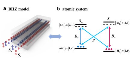
Figure 1: Mapping the BHZ model into an atomic system. (a) The BHZ model is a four-band tight-binding model in the basis $\{S_{+},S_{-}\}$, where the block $S_{+}=\{|+E_{1}\rangle,|+H_{1}\rangle\}$ is for the up-spin charge carriers and the block $S_{-}=\{|-E_{1}\rangle,|-H_{1}\rangle\}$ is for the down-spin charge carriers. The model exhibits a quantum spin Hall effect characterized by a helical edge state: the carriers with opposite spins move in opposite directions on a given edge. (b) Mapping the BHZ Hamiltonian into a four-level atomic system. In a cold ⁸⁷Rb atomic system, we encode the basis of the BHZ model with four atomic levels as follows: $|+E_{1}\rangle=|F=2,m_{F}=-1\rangle$, $|+H_{1}\rangle=|F=1,m_{F}=-1\rangle$, $|-E_{1}\rangle=|F=2,m_{F}=0\rangle$ and $|-H_{1}\rangle=|F=1,m_{F}=0\rangle$. The coefficients $\mathbf{B}_{+}$ and $\mathbf{B}_{-}$ in Eqs. (2) can be independently manipulated with $\pi$-transition microwaves, and the coupling term $g$ between $\{|+E_{1}\rangle,|-H_{1}\rangle\}$ $(\{|-E_{1}\rangle,|+H_{1}\rangle\})$ can be manipulated with $\sigma^{-}$ ($\sigma^{+}$)-transition microwaves.

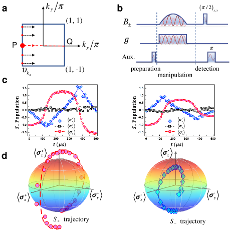
Figure 2: Detection method using the linear response theory and tomographic results. (a) The procedure of measuring the Berry curvature in the first Brillouin zone. Manipulation based on the linear response theory is realized by sweeping $k_{x}$ (along the black arrows) at each $k_{y}$ with a ratio $\upsilon_{k_{x}}$. (b) Pulse sequences in the experiments. The system is initially prepared with an equal superposition of the two lowest eigenstates. The effective Hamiltonian with the coefficients $\mathbf{B}_{\pm}$ can be realized with the control microwaves with time-varying amplitudes, frequencies, and phases. Intermediate couplings $g$ can be used to mimic the non-conversing spin current case. In the detection step, we measure the population of each pseudospin to extract the Berry curvature. Auxiliary pulses (labelled by Aux.) are used for preparation and detection. (c) Tomography of pseudospin $S_{\pm}$ which corresponds to parameter quenches along the line denoted by points $P$ and $Q$ in (a). Dashed and solid lines are theoretical simulations with the Schödinger equation using Hamiltonian (1). The evolving four-level state is divided into two pseudospins $S_{\pm}$. Diamonds, squares, and circles are experimental data. (d) Trajectories of pseudospins $S_{\pm}$ in (c). Dashed lines are theoretical simulations, and diamonds and circles are experimental data. Parameters: $M=2B$ and $g=0.15A$.

The BHZ model.– In a pioneer paper Bernevig2006 , Bernevig, Hughes, and Zhang proposed an effective model of the two-dimensional time-reversal-invariant topological insulator in HgTe/CdTe quantum wells as follows,

$$H_{\text{BHZ}}=\left(\begin{array}[]{cc}H_{+}&g\sigma_{x}\\ g\sigma_{x}&H_{-}\end{array}\right),$$ (1)

where $H_{\tau}=\mathbf{B}_{\tau}\cdot\vec{\sigma}$ ($\tau=+,-)$ with $\vec{\sigma}$ being the Pauli matrixes. The coefficients $\mathbf{B}_{\tau}$ are given by

$$\left\{\begin{split}\mathbf{B}_{+}=\mathbf{B}=(A\sin k_{x},-A\sin k_{y},M(\mathbf{k})),\\ \mathbf{B}_{-}=(-A\sin k_{x},-A\sin k_{y},M(\mathbf{k})),\\ M(\mathbf{k})=M-2B(2-\cos k_{x}-\cos k_{y}).\end{split}\right.$$ (2)

Here $A,M$, and $B$ are material parameters dependent on the quantum well geometry and the momentum ${k_{x},k_{y}}\in[-\pi,\pi]$. The $g$ describes the band coupling strength and this coupling term between blocks is determined by crystal symmetry and plays an important role in determining the spin orientation of the helical edge state XQi2011 . The basis in Eq. (1) is four subbands in the system and is ordered as $\{|+,E_{1}\rangle,|+,H_{1}\rangle,|-,E_{1}\rangle,|-,H_{1}\rangle\}$.

The topological properties of the BHZ model are well characterized by a SCN LSheng2005 . The physics can be easily understood when the coupling strength $g=0$. Under this condition, each pseudospin is conserved, and thus $H_{\text{BHZ}}$ consists of two decoupled blocks that are topologically equivalent to two copies of the Haldane model Haldane1988 . Each pseudospin has an independent CN $C_{+}$ and $C_{-}$ defined as $C_{\tau}=\frac{1}{2\pi}\int_{BZ}d\mathbf{k}\cdot\mathbf{\Omega_{\tau}}(\mathbf{k})$, where $\mathbf{\Omega_{\tau}}(\mathbf{k})=\mathbf{B}_{\tau}/|\mathbf{B}_{\tau}|$ is the Berry curvature in the first Brillouin zone (BZ). The time-reversal symmetry gives rise to a vanished total CN ( i.e., $C_{+}+C_{-}=0$). The difference

$$C_{s}=(C_{+}-C_{-})/2$$ (3)

is 1 for $M/2B>0$ and defines quantized spin Hall conductivity, and it is 0 for $M/2B<0$.

A fundamental result of the BHZ model is that the SCN can still be well defined when $\langle\sigma_{z}\rangle$ is non-conserved under the condition that two blocks are coupled. The energy gap of the system is defined as $\Delta_{cv}\equiv\mathrm{Min}(\mathcal{E}_{3}-\mathcal{E}_{1})=\mathrm{Min}|2\mathcal{E}_{1}|$, where the eigenvalues of the Hamiltonian (1) are obtained as $\mathcal{E}_{1}=\mathcal{E}_{2}=-\sqrt{B_{x}^{2}+B_{y}^{2}+B_{z}^{2}+g^{2}}$ and $\mathcal{E}_{3}=\mathcal{E}_{4}=-\mathcal{E}_{1}$. To calculate the spin spectrum gap, we first project the system to the subsystem spanned by the two lowest eigenstates $|\phi_{1,2}\rangle$ of $\mathcal{E}_{1,2}$, which induces a reduced Hamiltonian $H^{s}$ with $H^{s}_{jl}=\langle\phi_{j}|I\otimes\sigma_{z}|\phi_{l}\rangle,(j,l=1,2)$ with $I$ being the identity matrix. Through diagonalizing $H^{s}$ to obtain the eigenvalues $\mathcal{E}_{\pm}$ and the related eigenstates $|\psi_{\pm}\rangle$, we can define the spin spectrum gap $\Delta_{s}=|\mathcal{E}_{+}-\mathcal{E}_{-}|$ Prodan2009 ; LSheng2014 . Initially, it is found that the SCN may change its sign when the Hamiltonian is continuously deformed using spin rotation while the bulk gap is kept unchanged LFu2006 ; Fukui2007 . However, it has been shown that the SCN is well defined if both the energy gap and the spin spectrum gap are non-vanishing Prodan2009 . One can define a gauge potential $A_{k_{\mu}}^{\tau}\equiv\langle\psi_{\tau}|\partial_{k_{\mu}}|\psi_{\tau}\rangle$ and the related gauge field $F^{\tau}_{k_{x}k_{y}}\equiv\partial_{k_{x}}A^{\tau}_{k_{y}}-\partial_{k_{y}}A^{\tau}_{k_{x}}$. Integrating the spin Berry curvature defined by $F_{k_{x}k_{y}}^{s}=F_{k_{x}k_{y}}^{+}-F_{k_{x}k_{y}}^{-}$ over the BZ gives the SCN of the system

$$C_{s}=\frac{1}{2}\int_{\text{BZ}}F_{k_{x}k_{y}}^{s}dk_{x}dk_{y}$$ (4)

under the conditions $\Delta_{s}>0$ and $\Delta_{cv}>0$. For any $g$ in the BHZ model, the SCN is 1 for $M/2B>0$ and is 0 for $M/2B<0$, while $M/2B=0$ is a critical point of the topological phase transition. Because the eigenfunctions $|\psi_{\pm}\rangle$ are relevant to an artificially-constructed Hamiltonian $H^{s}$, not to the original Hamiltonian of the system, it is difficult to directly use definition (4) to measure the SCNs in a real condensed matter system, and thus the SCNs of a quantum system have not yet been experimentally observed. However, this problem can be solved in well-designed artificial quantum systems where wavefunctions of the reduced Hamiltonian $H^{s}$ can be created and manipulated.

Quantum simulation of the BHZ model with cold atoms.– As shown in Fig. 1 and deduced in detail in Supplemental Material (SM) SM , the BHZ model can be mapped into a four-level ⁸⁷Rb atomic system with the codes: $S_{+}=\{|+E_{1}\rangle=|F=2,m_{F}=-1\rangle,|+H_{1}\rangle=|F=1,m_{F}=-1\rangle\}$, $S_{-}=\{|-E_{1}\rangle=|F=2,m_{F}=0\rangle,|-H_{1}\rangle=|F=1,m_{F}=0\rangle\}$. The coefficients $\mathbf{B}_{\pm}$ and the coupling strength $g$ can be realized with the microwaves coupling the atomic energy levels. The ⁸⁷Rb atoms are evaporatively cooled down and then trapped in an optical dipole trap with atom number about $10^{6}$ and temperature about 10 $\mu$K. A magnetic field about 0.5 Gauss is applied along the $z$ direction as the quantization axis, which generates a $700$ kHz frequency difference between the two states’ energy level difference in $S_{+}$ and that in $S_{-}$. Thus, the quantum state of pseudospins $S_{+}$ and $S_{-}$ can be manipulated independently using $\pi$-transition microwaves. The $g\Pi_{+-}$ term between the pseudospins $\{|+E_{1}\rangle,|-H_{1}\rangle\}$ $(\{|-E_{1}\rangle,|+H_{1}\rangle\})$ can be manipulated with $\sigma^{-}$ ($\sigma^{+}$)-transition microwaves. In our system, the $1/e$ coherence time $T_{2}^{*}$ of $S_{+}$ ( magnetism-sensitive sublevel) is about 4 ms after stabilizing the quantization axis with active feedback control, while the coherence time $T_{2}^{*}$ of $S_{-}$ (magnetism-insensitive sublevel) is longer than 1 second. The system can operate under a maximal Rabi frequency of tens kHz Sugawa2018 , so it allows sufficiently fast manipulations and all manipulations can be finished within the decoherence times of $S_{+}$ and $S_{-}$.

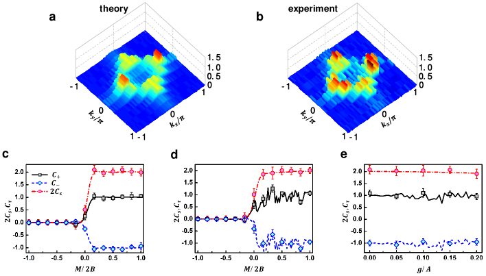
Figure 3: Spin Berry curvatures and SCNs. (a)(b) Spin Berry curvatures in the first Brillouin zone. (a) Theoretical simulation. The spin Berry curvature is computed by the difference between the Berry curvature of each pseudospin using the linear response theory with Eq. (5). (b) Experimental measurement. (c) SCNs $C_{s}$ and CN $C_{\pm}$ versus $M/2B$ with $g=0$. (d) $C_{s}$ and $C_{\pm}$ versus $M/2B$ with $g=0.15A$. A topological transition occurs at $M/2B=0$ in (c,d). (e) $C_{s}$ and $C_{\pm}$ against intermediate coupling $g$ at $M=2B$. Lines: theoretical curves computed by the linear response theory with Eq. (5). Circles, squares, and diamonds: experimental data. Red dashed-dotted lines with red circles: $C_{s}$. Black solid lines with black squares: $C_{+}$. Blue dashed lines with blue diamonds: $C_{-}$. The SCNs have been multiplied by a factor of 2. The error bars are standard error of the 4 measurements.

Measuring spin Berry curvature.– We now show that in this simulated BHZ model, the spin Berry curvature defined in the first BZ $k_{x},k_{y}\in[-\pi,\pi]$ can be detected using the linear response theory, which is given as the leading order correction to adiabatic manipulation.

Our measuring procedure is described in Fig. 2. In the experiments, we choose one $k_{y}$ in the set $\{k_{y}(q)=-\pi+\frac{\pi}{5}(q-1),q=1,...,11\}$, and then sweep $k_{x}$ (along the black arrows in Fig. 2(a)) at each $k_{y}$ with a ratio $v_{k_{x}}=2\pi/T$, i.e., $k_{x}(t)=v_{k_{x}}t-\pi$ with the time $t\in[0,T]$. The experiment sequence consists of preparation, manipulation, and detection steps, as shown in Fig. 2(b). In the preparation step, we prepare an initial state given by $|\Psi(0)\rangle=\left(\begin{array}[]{c}|\eta^{+}(0)\rangle\\ |\eta^{-}(0)\rangle\end{array}\right)$, and $\left(\begin{array}[]{c}1\\ 0\end{array}\right)\otimes|\eta^{+}(0)\rangle=|\phi_{1}(0)\rangle,\left(\begin{array}[]{c}0\\ 1\end{array}\right)\otimes|\eta^{-}(0)\rangle=|\phi_{2}(0)\rangle$, where $|\eta^{\tau}(t)\rangle$ is the wave function defined in pseudospin $S_{\tau}$ and $|\phi_{1,2}(0)\rangle$ are the two lower normalized eigenstates of the Hamiltonian $H(k_{x},k_{y})$ at $k_{x}=-\pi$ and $k_{y}=k_{y}(q)$ for a specific $q$. The whole wavefunction $|\Psi(0)\rangle$ is however normalized to $2$; that is, $\langle\Psi(t)|\Psi(t)\rangle=2$ since it is more convenient if the wavefunction of each pseudospin itself is normalized to one.

In the manipulation step, we sweep the Hamiltonian from $H(-\pi,k_{y}(q))$ to $H(k_{x}(t),k_{y}(q))$ by modulating the amplitudes, phases, and frequencies of the microwaves used to manipulate the atoms. To realize the BHZ Hamiltonian, the relative phases between the microwaves should be carefully determined by the interference of microwave driven Rabi oscillations. To mimic the non-conversing spin currents, the intermediate coupling $g$ is introduced and can be controlled by the amplitude of the microwave coupling between the pseudospins. To keep two-photon resonance condition with $B_{\pm}$, the frequencies of the intermediate coupling should also be swept. Following the method outlined in Ref.Gritsev2012 , we show in SM SM that the Berry curvature of pseudospin $S_{\tau}$ can be derived by

$$F_{k_{x}k_{y}}^{\tau}=\frac{\langle f_{k_{y}}^{\tau}\rangle-\langle f_{0}^{\tau}\rangle}{v_{k_{x}}},$$ (5)

where $\langle f_{k_{y}}^{\tau}\rangle=-\langle\partial_{k_{y}}H_{\tau}\rangle=A\cos k_{y}\langle\sigma_{y}^{\tau}\rangle+2B\sin k_{y}\langle\sigma_{z}^{\tau}\rangle$ ($\sigma^{\tau}_{x,y,z}$ are Pauli matrices for pseudospin $S_{\tau}$) and $\langle f_{0}^{\tau}\rangle=4B\sin k_{y}$. Therefore, the Berry curvature can be derived by tomographically measuring the expectation values $\langle\sigma^{\tau}_{y,z}\rangle$, which is described in detail in SM SM . As emphasized in SM SM , the expectation values $\langle\sigma^{\tau}_{x,y,z}\rangle$ are defined based on the pseudospin wavefunctions $|\eta^{\tau}(t)\rangle$.

In our experiments, the parameters are set to be $A=B=2\pi\times 24$ kHz and $T=500$ $\mu$s, which induce a nonadiabatic condition of $AT=BT=24\pi$, as discussed in SM SM . The experimental data $\langle\sigma_{x,y,z}^{\tau}\rangle$ are plotted in Fig. 2(c) when $(k_{x},k_{y})$ is swept from $(k_{x}(t=0),k_{y}(q))=(-\pi,0)$ with the parameters $M=2B$ and $g=0.15A$. From these data, we plot the evolution trajectories $\langle\sigma_{x,y,z}^{\tau}\rangle$ of $S_{\pm}$, where the red (blue) dashed lines are theoretical curves and red circles (blue diamonds) are experimental data of the pseudospins $S^{+}(S^{-})$. Since the intermediate couplings are non-vanishing, the evolution trajectories will be either inside or outside the Bloch spheres, which mimics the most interesting case of the non-conserving spin current in the BHZ model.

Here we show the results of the measuring Berry curvature. Typically, for $g=0$, the Berry curvature is symmetric along $k_{x}=0$ and $k_{y}=0$. At $q=6$, one obtain $M(k)=2B\cos k_{x}$ with zero frequency shift, and the pseudospins are driven from the north pole to the south pole (the trajectories are shown in SM SM ). By sweeping $k_{x}$ at each $k_{y}$ ($q$ from 1 to 11), the Berry curvature in the BZ can be derived from measured $\langle\sigma_{x,y,z}^{\tau}\rangle$. The theoretical simulation and experimental data of spin Berry curvature $F^{s}_{k_{x}k_{y}}=F^{+}_{k_{x}k_{y}}-F^{-}_{k_{x}k_{y}}$ under the condition of $M=2B$ and $g=0$ are plotted in Figs. 3(a) and 3(b).

SCNs and topological phase transition.– The SCN is obtained by integrating the spin Berry curvature over the first BZ with Eq. (4). In Fig. 3(c), we plot the measured $C_{s}$ and $C_{\tau}$ versus the parameter $M/2B$ with $g=0$. Theoretically, the BHZ model is in the topological insulating state when $M/2B>0$ and the trivial insulating state when $M/2B<0$. This topologically nontrivial-to-trivial transition has been confirmed in our experiments, as demonstrated in Fig. 3(c), where $C_{s}$ jumps from 1 to 0 at the critical point of $M/2B=0$. Although relatively large fluctuations are contained in the experimental results of the spin Berry curvature, the measured SCNs $C_{s}$ (red circles) and CNs $C_{\tau}$ (black squares and blue diamonds) are stable at 1 and $\pm 1$ respectively, as shown by Figs. 3(a) and 3(b). This suggests that the SCN is robust against the fluctuations introduced by the controls and measurements.

We will further demonstrate that using the linear response theory to measure the SCNs is also valid for the model with non-vanishing intermediate coupling $g$. In our experiment, the interaction strength is set to $g=0.15A$ and the method to prepare the initial state for $g\not=0$ is addressed in SM SM , while the control and measurement procedures are the same as with the case of $g=0$. As shown in Fig. 3(d), in the topological insulating region, the measured $C_{\tau}$ has large fluctuations, whereas, the SCN computed from the difference of $C_{\tau}$ is very stable. This clearly reveals that $C_{\tau}$ is not a well-defined topological invariant since it is not even an integer, but the SCN remains valid when intermediate coupling is present between the pseudospins. The above results meet the rigorous calculations using the U-linked method Fukui2007 , which confirms the validation of the linear response theory.

As demonstrated in Fig. 3(c) and 3(d), SCNs are robust against variations of the control parameters $M/2B$, and we further show that this robustness remains for the other parameter $g$. $C_{s}$ and $C_{\tau}$ versus $g$ for $M=2B$ are plotted in Fig. 3(e). As the pseudospin gap does not close, SCNs are stable with $C_{s}=1$, while $C_{\tau}$ numerically calculated with the linear response method fluctuates in this region. Therefore, combining the above results, we observe that SCNs are robust against the parameter variations ($g$ and $M$) as well as random fluctuations (i.e., fluctuations of the measured Berry curvature as shown in Fig. 3(b)).

Conclusions.– We have measured topological SCNs in a simulated BHZ model for the first time. Our observations can close the debate whether SCNs can be defined in a spin non-conserved system LFu2006 ; Fukui2007 ; Prodan2009 . The fully controllable Hamiltonian allows us to investigate other topological models, e.g., the Kane-Mele model Kane2005Z2 , by employing suitable coupling. Our work can be extended to other real or artificial atomic systems, including superconducting qubits, nitrogen-vacancy centers, quantum dots, and trapped ions Georgescu2014 . Since the linear response method used here is experimentally feasible, our work may lead to the detection of other topological invariants in condensed matter physics and artificial quantum systems. For example, with the spin Hall effect realized with ultracold atoms Beeler2013 ; SLZhu2006 , lattice extensions of our work Jotzu2014 ; LBShao2008 ; Goldman2016 ; Gianfrat2020 , together with the Feshbach resonance CChin2010 , may allow detection of topological invariants for an interacting bosonic or fermionic quantum gas in optical lattices SLZhu2013 ; QNiu1985 . Directly probing these topological invariants is essential for the advance of topological physics and its quantum simulations.

- (1) M. Z. Hasan and C. L. Kane, Rev. Mod. Phys. 82, 3045 (2010).
- (2) X. L. Qi and S. C. Zhang, Rev. Mod. Phys. 83, 1057 (2011).
- (3) D. W. Zhang, Y. Q. Zhu, Y. X. Zhao, H. Yan, and S. L. Zhu, Adv. Phys. 67, 253 (2018).
- (4) T. Ozawa, H. M. Price, A. Amo, N. Goldman, M. Hafezi, L. Lu, M. Rechtsman, D. Schuster, J. Simon, O. Zilberberg, and I. Carusotto, Rev. Mod. Phys. 91, 015006 (2019).
- (5) D. J. Thouless, M. Kohmoto, M. P. Nightingale, and M. den Nijs, Phys. Rev. Lett. 49, 405 (1982).
- (6) D. J. Thouless, Phys. Rev. B 27, 6083 (1983); Q. Niu and D. J. Thouless, J. Phys. A 17, 2453 (1984).
- (7) F. D. M. Haldane, Phys. Rev. Lett. 61, 2015 (1988).
- (8) C. L. Kane and E. J. Mele, Phys. Rev. Lett., 95, 226801 (2005).
- (9) C. L. Kane and E. J. Mele, Phys. Rev. Lett., 95, 146802 (2005).
- (10) D. N. Sheng, Z. Y. Weng, L. Sheng, and F. D. M. Haldane, Phys. Rev. Lett. 97, 036808 (2006).
- (11) L. Sheng, D. N. Sheng, C. S. Ting, and F. D. M. Haldane, Phys. Rev. Lett. 95, 136602 (2005).
- (12) L. Fu and C. L. Kane, Phys. Rev. B 74, 195312 (2006).
- (13) T. Fukui and Y. Hatsugai, Phys. Rev. B 75, 121403R (2007).
- (14) E. Prodan, Phys. Rev. B 80, 125327 (2009).
- (15) S. L. Zhu, Z.-D. Wang, Y.-H. Chan, and L.-M. Duan, Phys. Rev. Lett. 110, 075303 (2013).
- (16) L. Sheng, H. C. Li, Y. Y. Yang, D. N. Sheng, and D. Y. Xing, Chin. Phys. B 22, 067201 (2013).
- (17) D. Carpentier, P. Delplace, M. Fruchart, and K. Gawedzki, Phys. Rev. Lett. 114, 106806 (2015).
- (18) L. M. Canonico, T. G. Rappoport, and R.B. Muniz, Phys. Rev. Lett. 122, 196601 (2019).
- (19) C. Z. Chen, H. Liu, and X. C. Xie, Phys. Rev. Lett. 122, 026601 (2019).
- (20) L. Sheng, Progress in Physics, 34, 10 (2014).
- (21) B. A. Bernevig, T. L. Hughes, and S. C. Zhang, Science, 314, 1757 (2006).
- (22) M. Konig, S. Wiedmann, C. Brune, A. Roth, H. Buhmann, L. W. Molenkamp, X. L. Qi, and S. C. Zhang, Science, 318, 766 (2007).
- (23) D. Hsieh, D. Qian, L. Wray, Y. Xia, Y. S. Hor, R. J. Cava, and M. Z. Hasan, Nature, 452, 979 (2008).
- (24) D. Hsieh, Y. Xia, L. Wray, D. Qian, A. Pal, J. H. Dil, J. Osterwalder, F. Meier, G. Bihlmayer, C. L. Kane, Y. S. Hor, R. J. Cava, and M. Z. Hasan, Science, 323, 919 (2009).
- (25) M. Aidelsburger, M. Lohse, C. Schweizer, M. Atala, J. T. Barreiro, S. Nascimbène, N. R. Cooper, I. Bloch, and N. Goldman, Nat. Phys. 11, 162 (2015).
- (26) L. Duca, T. Li, M. Reitter, I. Bloch, M. Schleier-Smith, and U. Schneider, Science 347, 288 (2015).
- (27) X. Tan, D. W. Zhang, Z. Yang, J. Chu, Y. Q. Zhu, D. Li, X.Yang, S. Song, Z. Han, Z. Li, Y. Dong, H.F. Yu, H. Yan, S. L. Zhu, and Y. Yu, Phys. Rev. Lett. 122, 210401 (2019).
- (28) M. Yu, P. Yang, M. Gong, Q. Cao, Q. Lu, H. Liu, S. Zhang, M. B. Plenio, F. Jelezko, T. Ozawa, N. Goldman, and J. Cai, National Science Review 7, 254 (2020).
- (29) X. Tan, D. W. Zhang, Q. Liu, G. Xue, H. F. Yu, Y. Q. Zhu, H. Yan, S. L. Zhu, and Y. Yu, Phys. Rev. Lett. 120, 130503 (2018).
- (30) T. Li, L. Duca, M. Reitter, F. Grusdt, E. Demler, M. Endres, M. Schleier-Smith, I. Bloch and U. Schneider, Science 352 1094 (2016).
- (31) S. Sugawa, F. Salces-Carcoba, A. R. Perry, Y. C. Yue, and I. B. Spielman, Science 360, 1429 (2018).
- (32) P. Roushan, C. Neill, Y. Chen, M. Kolodrubetz, C. Quintana, N. Leung, M. Fang, R. Barends, B. Campbell, Z. Chen, B. Chiaro, A. Dunsworth, E. Jeffrey, J. Kelly, A. Megrant, J. Mutus, P. O’Malley, D. Sank, A. Vainsencher, J. Wenner, T. White, A. Polkovnikov, A. N. Cleland, and J. M. Martinis, Nature (London) 515, 241 (2014).
- (33) C. Schweizer, M. Lohse, R. Citro, and I. Bloch, Phys. Rev. Lett. 117, 170405 (2016).
- (34) M. Lohse, C. Schweizer, H. M. Price, O. Zilberberg, and I. Bloch, Nature 553, 55 (2018).
- (35) See Supplemental Material for details on the theoretical model, experimental setup, measurement and data processing.
- (36) V. Gritseva and A. Polkovnikovb, Proc. Natl. Acad. Sci. 109, 17 (2012).
- (37) I. M. Georgescu, S. Ashhab, and Franco Nori, Rev. Mod. Phys. 86, 153 (2014).
- (38) M. C. Beeler, R. A. Williams, K. Jimenez-Garcia, L. J. LeBlanc, A. R. Perry, and I. B. Spielman, Nature (London) 498, 201 (2013).
- (39) S. L. Zhu, H. Fu, C. J. Wu, S. C. Zhang, and L. M. Duan, Phys. Rev. Lett. 97, 240401 (2006).
- (40) G. Jotzu, M. Messer, R. Desbuquois, M. Lebrat, T. Uehlinger, D. Greif, and T. Esslinger, Nature (London) 515, 237 (2014).
- (41) L. B. Shao, S. L. Zhu, L. Sheng, D. Y. Xing, and Z. D. Wang, Phys. Rev. Lett. 101, 246810 (2008).
- (42) N. Goldman, J. C. Budich, and P. Zoller, Nature Phys.12, 639 (2016).
- (43) A. Gianfrate, O. Bleu, L. Dominici, V. Ardizzone, M. De Giorgi, D. Ballarini, G. Lerario, K. W. West, L. N. Pfeiffer, D. D. Solnyshkov, D. Sanvitto, and G. Malpuech, Nature 578, 381 (2020).
- (44) C. Chin, R. Grimm, P. Julienne, and E. Tiesinga, Rev. Mod. Phys. 82 1225 (2010).
- (45) Q. Niu, D.J. Thouless, and Y.S. Wu, Phys. Rev. B 31, 3372 (1985).