Discrete Lehmann representation of imaginary time Green’s functions

Abstract

We present an efficient basis for imaginary time Green’s functions based on a low rank decomposition of the spectral Lehmann representation. The basis functions are simply a set of well-chosen exponentials, so the corresponding expansion may be thought of as a discrete form of the Lehmann representation using an effective spectral density which is a sum of $\delta$ functions. The basis is determined only by an upper bound on the product $\beta\omega_{\max}$, with $\beta$ the inverse temperature and $\omega_{\max}$ an energy cutoff, and a user-defined error tolerance $\epsilon$. The number $r$ of basis functions scales as $\mathcal{O}\left(\log(\beta\omega_{\max})\log\left(1/\epsilon\right)\right)$. The discrete Lehmann representation of a particular imaginary time Green’s function can be recovered by interpolation at a set of $r$ imaginary time nodes. Both the basis functions and the interpolation nodes can be obtained rapidly using standard numerical linear algebra routines. Due to the simple form of the basis, the discrete Lehmann representation of a Green’s function can be explicitly transformed to the Matsubara frequency domain, or obtained directly by interpolation on a Matsubara frequency grid. We benchmark the efficiency of the representation on simple cases, and with a high precision solution of the Sachdev-Ye-Kitaev equation at low temperature. We compare our approach with the related intermediate representation method, and introduce an improved algorithm to build the intermediate representation basis and a corresponding sampling grid.

I Introduction

Quantum many-body physics is entering a new era, with the rise of high precision algorithms capable of obtaining controlled solutions in the strongly interacting regime. A large family of approaches concentrates on computing finite temperature correlation functions. Indeed, the imaginary time formalism in thermal equilibrium is well suited to describe both the thermodynamic and many of the equilibrium properties of a system.Abrikosov:QFT It is widely used, for example by quantum Monte Carlo algorithms, which are formulated in imaginary time.

For many applications, generic methods of representing one and two-particle imaginary time Green’s functions may be insufficient to obtain the required precision given computational cost and memory constraints. Examples include (i) the storage of one-body Green’s functions with a large number of orbitals, as in quantum chemistry applications (see Ref. GullStrand_2020, and the references therein), or on a lattice with complex momentum dependence; (ii) the high precision solution of the Dyson equation for such Green’s functions; (iii) computations in which highly accurate representations of Green’s functions are required, as for the bare propagator in some high-order perturbative expansions qqmc2020 ; and (iv) the storage of two-body Green’s functions, which depend on three time arguments shinaoka18 ; shinaoka20 .

The simplest approach is to represent a Green’s function $G$ on a uniform grid of $m$ points in imaginary time $\tau$, and by a truncated Fourier series of $m$ modes in Matsubara frequency $i\nu_{n}$. While this method offers some practical advantages, including the ability to transform between the imaginary time and Matsubara frequency domains by means of the fast Fourier transform, it is a poor choice from the point of view of efficiency, particularly when the inverse temperature $\beta$ is large. First, $m=\mathcal{O}\left(\beta\right)$ grid points are required in imaginary time to resolve sharp features caused by high energy scales. Second, since the Green’s functions are discontinuous at the endpoints $\tau=0$ and $\beta$ of the imaginary time interval, their Fourier coefficients decay as $\mathcal{O}\left(1/m\right)$, so that the representation converges with low-order accuracy.

Representing $G(\tau)$ by an orthogonal polynomial (Chebyshev or Legendre) expansion of degree $m$ yields a significant improvement.Boehnke2011 Indeed, since $G(\tau)$ is smooth on $[0,\beta]$, such a representation converges with spectral accuracy Boehnke2011 ; kananenka16 ; gull18 ; gull18 ; GullStrand_2020 ; see also Ref. trefethen19, for a thorough overview of the theory of orthogonal polynomial approximation. However, resolving the Green’s function still requires an expansion of degree $m=\mathcal{O}\left(\sqrt{\beta}\right)$. chikano18

A third idea is the “power grid” method, which uses a grid exponentially clustered towards $\tau=0$ and $\beta$. In this approach, an adaptive sequence of panels is constructed, and a polynomial interpolant used on each panel, leading to a representation requiring only $\mathcal{O}\left(\log\beta\right)$ degrees of freedom. ku00 ; ku02 ; kananenka16 However, the power grid method has been implemented using uniform grid interpolation on each panel, which can lead to numerical instability for high-order interpolants. A more stable method, using spectral grids on each panel, is incorporated as an intermediate step in our framework, but ultimately further compression of the representation can be achieved.

A newer approach is to construct highly compact representations by taking advantage of the specific structure of imaginary time Green’s functions, which satisfy the spectral Lehmann representation

$$G(\tau)=-\int_{-\infty}^{\infty}K(\tau,\omega)\rho(\omega)\,d\omega,$$ (1)

for $\tau\in[0,\beta]$. Here $\rho$ is the spectral density, $\omega$ is a real frequency variable, and the kernel $K$ is given in the fermionic case by

$$K(\tau,\omega)=\frac{e^{-\omega\tau}}{1+e^{-\beta\omega}}.$$ (2)

In our discussion, we assume that the support of $\rho$ is contained in $[-\omega_{\max},\omega_{\max}]$, for $\omega_{\max}$ a high energy cutoff; this always holds to high accuracy for sufficiently large $\omega_{\max}$. For convenience, we also define a dimensionless high energy cutoff $\Lambda\equiv\beta\omega_{\max}$.

The key observation is that the fermionic kernel $K$ can be approximated to high accuracy by a low rank decomposition. shinaoka17 The most well-known manifestation of this fact is the severe ill-conditioning of analytic continuation from the imaginary to the real time axis. However, one can take advantage of this low rank structure to obtain a compact representation of $G(\tau)$. In Refs. shinaoka17, ; chikano18, , orthogonal bases for imaginary time Green’s functions containing only $\mathcal{O}\left(\log\Lambda\right)$ basis functions are constructed from the left singular vectors in the singular value decomposition (SVD) of a discretization of $K$. This method, called the intermediate representation (IR), has been used successfully in a variety of applications, including those involving two-particle quantities shinaoka18 ; shinaoka19 ; otsuki20 ; shinaoka20 ; wallerberger20 ; wang20 ; shinaoka21 ; see also Ref. shinaoka21_2, for a useful review and further references. A related approach is the minimax isometry method, which uses similar ideas to construct optimal quadrature rules for Matsubara summation in GW applications. kaltak20

In this paper, we present a method which is related to the IR, but uses a different low rank decomposition of $K$, called the interpolative decomposition (ID). cheng05 ; liberty07 It leads to a discrete Lehmann representation (DLR) of any imaginary time Green’s function $G(\tau)$ as a linear combination of $r$ exponentials $e^{-\omega_{k}\tau}$ with a set of frequencies $\omega_{k}$ which depend only on $\Lambda$ and $\epsilon$. Like the IR basis, the DLR basis is universal in the sense that given any $\Lambda$ and $\epsilon$, it is sufficient to represent any imaginary time Green’s function obeying the energy cutoff $\Lambda$ to within accuracy $\epsilon$. The number of basis functions is observed to scale as $r=\mathcal{O}\left(\log(\Lambda)\log\left(1/\epsilon\right)\right)$, and is nearly the same as the number of IR basis functions with the same choice of $\Lambda$ and error tolerance $\epsilon$.

Our construction begins with a discretization of $K$ on a composite Chebyshev grid, designed to resolve the range of energy scales present in Green’s functions up to a given cutoff $\Lambda$. Then, instead of applying the SVD to the resulting matrix as in the IR method, we use the ID to select a set of $r$ representative frequencies $\omega_{k}$ such that the functions $K(\tau,\omega_{k})$ form the basis of exponentials. The ID also yields a set of $r$ interpolation nodes, such that the DLR of a given Green’s function $G$ can be recovered from samples at those nodes. The DLR can be explicitly transformed to the Matsubara frequency domain, where it takes the form of a linear combination of $r$ poles $(i\nu_{n}+\omega_{k})^{-1}$. As in the imaginary time domain, the DLR can also be recovered by interpolation at $r$ nodes on the Matsubara frequency axis.

Compared with the IR approach, the DLR basis exchanges orthogonality for a simple, explicit form of the basis functions. However, we show that orthogonality is not required for numerically stable recovery of the representation. On the other hand, using an explicit basis of exponentials has many advantages. In particular, it avoids the cost and complexity of working with the IR basis functions, which are themselves represented on a fine adaptive grid, and evaluated using corresponding interpolation procedures. Many standard computational tasks – such as transforming between the imaginary time and Matsubara frequency domains, and performing convolutions – are reduced to simple explicit formulas.

The algorithms which we use in the context of the DLR also carry over to the IR method, and offer two main improvements over previously established algorithms.

First, the numerical tools we describe can be used to construct an efficient sampling grid for the IR basis in a more systematic manner than the sparse sampling method, which is typically used. Sparse sampling provides a method of obtaining compact grids in imaginary time and Matsubara frequency, from which one can recover the IR coefficients. li20 The sparse sampling grid is analogous to the interpolation grid used for the DLR. However, whereas the sparse sampling method selects a grid based on a heuristic, we use a purely linear algebraic method with robust accuracy guarantees, which is also applicable to the IR.

Second, existing methods to build the IR basis functions are computationally intensive, requiring hours of computation time for large values of $\Lambda$. Furthermore, the basis functions themselves are represented using a somewhat complicated adaptive data structure. Of course, basis functions for a given choice of $\Lambda$ need only be computed once and stored, and to facilitate the process, an open source software package has been released which contains tabulated basis functions for several fixed values of $\Lambda$, as well as routines to work with them. chikano19 However, in some cases, the situation is cumbersome, for example if one wishes to converge a calculation with respect to $\Lambda$. By contrast, we present a simple discretization of $K(\tau,\omega)$, which allows us to construct either the DLR or IR basis functions from a single call to the pivoted QR and SVD algorithms, respectively, with matrices of modest size. This yields the basis functions and associated imaginary time interpolation nodes in less than a second on a laptop for $\Lambda$ as large as $10^{6}$ and $\epsilon$ near the double machine precision. The resulting DLR basis functions are characterized by a list of $r$ frequency nodes $\omega_{k}$, and the IR basis functions are represented using a simple data structure.

In addition to describing efficient algorithms to implement the DLR, we present mathematical theorems which provide error bounds and control inequalities. We illustrate the DLR approach on several simple examples, as well as on a high precision, low temperature solution of the Sachdev-Ye-Kitaev (SYK) model. SachdevYe93 ; gu20

Open source Fortran and Python implementations of the DLR are available in the library libdlr.libdlr We refer the reader to Ref. kaye21, for a detailed description.

This paper is structured as follows. In Section II, we present a short overview of the DLR with an example, leaving aside technical details. In Section III, we introduce the mathematical tools required in the rest of the paper, namely composite Chebyshev interpolation and the interpolative decomposition. In Section IV, we develop the DLR, describe our algorithm, and show some benchmarks. In Section V, we derive the IR, describe its relationship with the DLR, and present efficient algorithms to construct the IR basis functions and associated grid. We show how to solve the Dyson equation efficiently using the DLR in Section VI, and demonstrate the method by solving the SYK equation in Section VII. Section VIII contains a concluding discussion.

II Overview

We develop our method using the fermionic kernel $K$; we show in Appendix A that in fact this kernel can also be used for bosonic Green’s functions. To simplify the notation, we also restrict our discussion to scalar-valued Green’s functions, as the extension to the matrix-valued case is straightforward.

We assume the spectral density $\rho$, which may in general be a distribution, is integrable and supported in $[-\omega_{\max},\omega_{\max}]$. It is convenient to further nondimensionalize (1) by performing the change of variables $\tau\leftarrow\tau/\beta$ and $\omega\leftarrow\beta\omega$. In these variables, we have $\tau\in[0,1]$, and the support of $\rho(\omega)$ is contained in $[-\Lambda,\Lambda]$, with $\Lambda=\beta\omega_{\max}$. $\Lambda$ is a user-determined parameter. An estimate of $\omega_{\max}$, and therefore of $\Lambda$, can often be obtained on physical grounds, but in general $\Lambda$ is used as an accuracy parameter and is increased until convergence is reached. Then, assuming $\Lambda$ is taken sufficiently large, (1) is equivalent to the truncated Lehmann representation

$$G(\tau)=-\int_{-\Lambda}^{\Lambda}K(\tau,\omega)\rho(\omega)\,d\omega,$$ (3)

for $K$ given by (2) with $\beta=1$.

As for the IR, we exploit the low numerical rank of an appropriate discretization of $K$ to obtain a compact representation of $G$. We simply use the ID, rather than the SVD, after discretizing $K$ on a carefully constructed grid. We will show that $G(\tau)$ can be approximated to any fixed accuracy $\epsilon$ by a discrete sum with $r$ terms,

$$G(\tau)\approx G_{\text{DLR}}(\tau)\equiv\sum_{k=1}^{r}K(\tau,\omega_{k})\widehat{g}_{k}.$$ (4)

Here $\{\omega_{k}(\Lambda,\epsilon)\}_{k=1}^{r}$ is a collection of selected frequencies, and the spectral density $\rho$ has been replaced by a discrete set of coefficients $\widehat{g}_{k}$. A minus sign has been absorbed into the coefficients to simplify expressions. The basis functions of this representation are simply exponentials,

$$G_{\text{DLR}}(\tau)=\sum_{k=1}^{r}\frac{e^{-\omega_{k}\tau}}{1+e^{-\omega_{k}}}\widehat{g}_{k}=\sum_{k=1}^{r}\widetilde{g}_{k}e^{-\omega_{k}\tau},$$ (5)

a feature which simplifies many calculations. We refer to (4, 5) as a discrete Lehmann representation of $G$.

We emphasize that given a user-specified error tolerance $\epsilon$ and a choice of $\Lambda$, the $r$ selected frequencies $\omega_{k}$ are universal; that is, independent of $G$. Furthermore, $r$, which we refer to as the DLR rank, is close to the $\epsilon$-rank of $K(\tau,\omega)$, which is the number of IR basis functions for the same choice of $\Lambda$ and $\epsilon$, so the DLR also requires at most $\mathcal{O}\left(\log(\Lambda)\log\left(1/\epsilon\right)\right)$ degrees of freedom. The high energy cutoff $\Lambda$ plays an important role in this representation, as it controls the regularity of $G(\tau)$, allowing a representation by a finite combination of exponentials. We will prove the existence of a representation (4) with error tightly controlled by $\epsilon$, and describe a method to construct such a representation by interpolation of $G$ at $r$ selected nodes in imaginary time or Matsubara frequency.

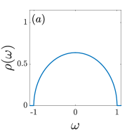
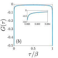
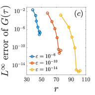
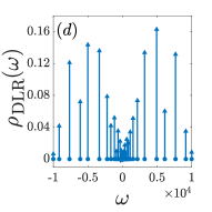
Figure 1: (a) Spectral density $\rho(\omega)=\frac{2}{\pi}\sqrt{1-\omega^{2}}\,\theta(1-\omega^{2})$. (b) Corresponding imaginary time Green’s function $G(\tau)$ with $\beta=10^{4}$. (c) $\norm{G-G_{\text{DLR}}}_{\infty}$ as a function of the number of basis functions $r$ for $\epsilon=10^{-6},10^{-10},10^{-14}$. The values of $r=r(\Lambda,\epsilon)$ correspond to $\Lambda=0.2\times 10^{4},0.4\times 10^{4},\ldots,1.2\times 10^{4}$. (d) Representation of the DLR coefficients $\widehat{g}_{k}$ as an effective spectral density which is a sum of $\delta$ functions, as in (6).

A first example is presented in Figure 1. We take $\beta=10^{4}$, and consider a particle-hole symmetric fermionic Green’s function $G(\tau)$ defined by the spectral density $\rho(\omega)=\frac{2}{\pi}\sqrt{1-\omega^{2}}\,\theta(1-\omega^{2})$, with $\theta$ the Heaviside function, as shown in Figures 1a and 1b. Figure 1c shows the error of the DLR (4, 5) as a function of $r$ for fixed $\epsilon=10^{-6},10^{-10},10^{-14}$. Here, we vary $\Lambda$ near the known sufficient value of $10^{4}$ ($\beta=10^{4}$ and $\rho$ is supported in $[-1,1]$) and plot the error here versus $r(\Lambda)$, instead of $\Lambda$, to emphasize the number of basis functions. The error decays super-exponentially at first, and reaches $\epsilon$ when $\Lambda\approx 10^{4}$. The value of $r$ at which convergence is reached depends on $\epsilon$, so that in practice, to obtain the smallest possible basis for a given accuracy, one should first choose $\epsilon$ and then increase $\Lambda$ until convergence.

The DLR can be formally interpreted as a spectral representation with an effective spectral density $\rho_{\text{DLR}}$ which is a sum of $\delta$ functions:

$$\rho_{\text{DLR}}(\omega)=-\sum_{k=1}^{r}\widehat{g}_{k}\delta(\omega-\omega_{k}).$$ (6)

Such a representation is made possible by the ill-conditioning of the integral operator defining the Lehmann representation; up to a fixed precision $\epsilon$, the spectral density corresponding to a given imaginary time Green’s function is highly non-unique. Thus, we simply pick one such spectral density with a particularly simple form, rather than attempting to reconstruct the original spectral density. Figure 1d shows a graphical representation of $\rho_{\text{DLR}}$ and hence of the coefficients $\widehat{g}_{k}$ and the selected frequencies $\omega_{k}$.

III Mathematical preliminaries

This section will review our two main numerical tools: composite Chebyshev interpolation, which will be used to obtain an accurate initial discretization of the kernel $K(\tau,\omega)$, and the interpolative decomposition, which will be used for low rank compression.

III.1 Composite Chebyshev interpolation

Polynomial interpolation at Chebyshev nodes is a well-conditioned method for the approximation of a smooth function $f$ on an interval. trefethen19 If $f$ can be analytically continued to a neighborhood of $[a,b]$, the error of the interpolant in the supremum norm decreases geometrically with its degree, and if $f$ can be analytically continued to the entire complex plane, the convergence is super-geometric; see Ref. trefethen19, (Thm. 8.2). There are fast and stable algorithms to evaluate Chebyshev interpolants, such as the method of barycentric Lagrange interpolation. berrut04 ; higham04

For functions with sharp features or variation at multiple length scales, using a single polynomial interpolant on $[a,b]$ is inefficient. A better alternative is to construct a piecewise polynomial interpolant by the method of composite Chebyshev interpolation at fixed order. To be precise, let $[a_{1},b_{1}],[a_{2},b_{2}],\ldots,[a_{n},b_{n}]$ with $a=a_{1}<b_{1}=a_{2}<b_{2}=\cdots=a_{n}<b_{n}=b$ be a collection of subintervals partitioning $[a,b]$. Let $\{x_{ij}\}_{i=1}^{p}$ be the $p$ Chebyshev nodes on $[a_{j},b_{j}]$. Then $\{x_{ij}\}_{{i,j=1}}^{p,n}$ is called a composite Chebyshev grid. Let $\ell_{ij}(x)$ be the Lagrange polynomial corresponding to the $i$th grid point on the $j$th panel; this is the polynomial of degree $p-1$ which satisfies

$$\ell_{ij}(x)=\begin{cases}1&\text{if }x=x_{ij}\\ 0&\text{if }x=x_{kj},k\neq i.\end{cases}$$

Let $\chi_{j}(x)$ be the characteristic function on the interval $[a_{j},b_{j}]$. Then the degree $p-1$ composite Chebyshev interpolant of a function $f$ on $[a,b]$ corresponding to the above partition is given by

$$\widehat{f}(x)=\sum_{j=1}^{n}\chi_{j}(x)\sum_{i=1}^{p}\ell_{ij}(x)f(x_{ij}).$$ (7)

Evidently, we have $f(x_{ij})=\widehat{f}(x_{ij})$ for each $i=1,\ldots,p$ and $j=1,\ldots,n$. The partition of $[a,b]$ should be chosen to resolve local features of $f$, and the degree $p$ should be chosen sufficiently large so that the rapidly converging Chebyshev interpolants of $f$ on each subinterval $[a_{j},b_{j}]$ are accurate.

To simplify expressions, we define the truncated Lagrange polynomial on the interval $[a_{j},b_{j}]$ by $\overline{\ell}_{ij}\equiv\ell_{ij}\chi_{j}$. It will also sometimes be convenient to cast the double index $i=1,\ldots,p$, $j=1,\ldots,n$ for the composite grid points to a single index $i=1,\ldots,p\times n$, with $x_{i}\leftarrow x_{ij}$, $\ell_{i}\leftarrow\ell_{ij}$, and $\overline{\ell}_{i}\leftarrow\overline{\ell}_{ij}$. In this notation, (7) becomes

$$\widehat{f}(x)=\sum_{i=1}^{p\times n}\overline{\ell}_{i}(x)f(x_{i}).$$ (8)

III.2 Interpolative decomposition

We say an $m\times n$ matrix $A$ is numerically low rank, or more specifically, has low $\epsilon$-rank, if $A$ has only $r\ll\min(m,n)$ singular values larger than $\epsilon$. The best rank $r$ approximation of $A$ in the spectral norm is given by its SVD truncated to the first $r$ singular values, and its error in that norm is the next singular value $\sigma_{r+1}$; see Ref. ballani16, (Sec. 2, Thm. 2). Thus, the truncated SVD (TSVD) yields an approximation with error $\epsilon$ in the spectral norm for a matrix with $\epsilon$-rank $r$.

The interpolative decomposition is an alternative to the TSVD for compressing numerically low rank matrices. It has the advantage that the column space is represented by selected columns of $A$, rather than an orthogonalization of the columns of $A$, as in the TSVD. The price is a mild and controlled loss of optimality compared with the TSVD. The ID and related algorithms are described in Refs. cheng05, ; liberty07, ; gu96, ; in particular, we make use of the form of the ID and the theoretical results summarized in Ref. liberty07, .

Given $A\in\mathbb{C}^{m\times n}$, the rank $r$ ID is given by

$$A\approx BP$$

with $B\in\mathbb{C}^{m\times r}$ a matrix containing $r$ selected columns of $A$, and $P\in\mathbb{C}^{r\times n}$, the so-called projection matrix, containing the coefficients required to approximately recover all of the columns of $A$ from the $r$ selected columns. The error of the decomposition is given by

$$\norm{A-BP}_{2}\leq\sqrt{r(n-r)+1}\,\sigma_{r+1},$$ (9)

so the ID gives a rank $r$ approximation of $A$ which is at most a factor of $\sqrt{r(n-r)+1}$ less accurate than the TSVD. The numerical stability of the ID as a representation of $A$ can also be guaranteed; in particular, we have

$$\norm{P}_{2}\leq\sqrt{r(n-r)+1}.$$ (10)

The references given above contain detailed statements of the relevant results which we have quoted here, along with the accompanying analysis.

Numerical algorithms are available which construct such a decomposition with bounds typically within a small factor of those stated above. The standard algorithm, described in Ref. cheng05, , proceeds in two steps. First, the pivoted QR process is applied to $A$, yielding a collection of $r$ columns of $A$ – corresponding to the pivot indices – which are, in a certain sense, as close as possible to being mutually orthogonal. These $r$ columns comprise the matrix $B$ in the ID. Next, a linear system is solved to determine the coefficients of the remaining columns of $A$ in the basis determined by $B$. These coefficients are stored in the matrix $P$. The cost of this algorithm is $\mathcal{O}\left(rmn\right)$. If the rank $r$ is not known a priori, it is straightforward to apply this algorithm in a rank-revealing manner, so that given an input $\epsilon$ it yields an estimated $\epsilon$-rank $r$ and a rank $r$ ID with $\norm{A-BP}_{2}\leq\epsilon$. Of course, the returned $\epsilon$-rank may be larger than the true $\epsilon$-rank, consistent with the suboptimality of the estimate (9) and the behavior of the singular values of $A$.

We remark that for several of the algorithms presented in this article – in particular for all the algorithms involving the DLR – we only ever need to perform the pivoted QR step of the ID to identify $k$ selected columns of a matrix, and in particular do not need to construct the full ID. Nevertheless, the presentation in terms of the ID is both conceptually and theoretically useful, and helps to unify our discussions of the DLR and the IR, so we adopt that language throughout. Our descriptions of algorithms in the text will make this point clear.

The Fortran library ID provides an implementation of the ID algorithm. idlib ; iddoc A Python interface is available in SciPy. idlibscipy For our numerical experiments, we use the implementation of the rank-revealing pivoted QR algorithm contained in the Fortran version of the library.

IV Discrete Lehmann representation

The DLR basis functions are built by a two-step procedure. First, we discretize $K(\tau,\omega)$ on a composite Chebyshev fine grid $\{(\tau_{i}^{f},\omega_{j}^{f})\}_{i=1,j=1}^{M,N}$, obtaining a matrix with entries $K(\tau_{i}^{f},\omega_{j}^{f})$. Then, we obtain a small subset $\{\omega_{l}\}_{l=1}^{r}$ of the fine grid points in $\omega$ from the ID of this matrix, such that

$$K(\tau,\omega)\approx\sum_{l=1}^{r}K(\tau,\omega_{l})\pi_{l}(\omega)$$ (11)

holds to high accuracy uniformly in $\tau$, for some coefficients $\pi_{l}(\omega)$. The functions $\{K(\tau,\omega_{l})\}_{l=1}^{r}$ are referred to as the DLR basis functions. Inserting (11) into the Lehmann representation (1) will establish the existence of the DLR. The discretization of $K$ will be discussed in Section IV.1, and the construction of the DLR basis in Section IV.2. In Sections IV.3 and IV.4, we will describe a stable method of constructing the DLR of a Green’s function $G$ from samples of $G$ at only $r$ selected imaginary time and Matsubara frequency nodes, respectively. In Section IV.5 we will give a practical summary of the various procedures, and we will demonstrate the DLR with a few simple examples in Section IV.6. Throughout the discussion, except when describing specific physical examples, we will work in the nondimensionalized variables described at the beginning of Section II, with $\tau\in[0,1]$, $\omega\in[-\Lambda,\Lambda]$, and $K(\tau,\omega)=e^{-\tau\omega}/(1+e^{-\omega})$.

IV.1 Discretization of $K(\tau,\omega)$

We discretize $K(\tau,\omega)$ by finding grids sufficient to resolve $K(\tau,\omega_{0})$ on $\tau\in[0,1]$ for all fixed $\omega_{0}\in[-\Lambda,\Lambda]$, and $K(\tau_{0},\omega)$ on $\omega\in[-\Lambda,\Lambda]$ for all fixed $\tau_{0}\in[0,1]$. A closely related problem was considered in Ref. gimbutas20, , in which it is shown (Lemma 4.4) that all exponentials in the family $\{e^{-\omega\tau}\}_{\omega\in[1,\Lambda]}$ can be represented to error uniformly less than $\epsilon$ on $\tau\geq 0$ in a basis of $\mathcal{O}\left(\log(\Lambda)\log\left(1/\epsilon\right)\right)$ exponentials chosen from the family. As in their proof, we will make use of dyadically refined composite Chebyshev grids. A minor modification of their proof is sufficient to give a rigorous justification of our method, though we do not discuss the details here.

We begin with the first case, for $\omega_{0}\in[0,\Lambda]$, which gives $K(\tau,\omega_{0})=ce^{-\omega_{0}\tau}$ for a constant $c$; a family of decaying exponentials. Consider the composite Chebyshev grid on $\tau\in[0,1]$ dyadically refined towards the origin; that is, with intervals given by $a_{1}=0$, $a_{i}=b_{i-1}=2^{-(m-i+1)}$ for $i=2,\ldots,m$, and $b_{m}=1$. We take $m\sim\log_{2}\Lambda$ to resolve the smallest length scale in the family of exponentials, which appears for $\omega_{0}=\Lambda$. With this choice, the degree parameter $p$ can be chosen sufficiently large so that the resulting composite Chebyshev interpolant is uniformly accurate for any $\Lambda$. Double precision machine accuracy $\epsilon_{\mbox{\tiny mach}}$ can be achieved with a moderate choice of $p$, since the Chebyshev interpolants of the exponentials converge rapidly with $p$. The accuracy of the interpolants can be checked directly, and $p$ refined to convergence.

For $\omega_{0}\in[-\Lambda,0]$, we observe that $K(\tau,\omega_{0})=ce^{\omega_{0}(1-\tau)}$, revealing a symmetry in $K$ about $\tau=1/2$. We therefore split the last interval $[1/2,1]$ in our partition into a set of subintervals dyadically refined towards $\tau=1$, in the same manner as above. The resulting composite Chebyshev grid is sufficient to resolve $K(\tau,\omega_{0})$ for all $\omega_{0}\in[-\Lambda,\Lambda]$, and contains $\mathcal{O}\left(\log\Lambda\right)$ points. An example of such a grid is shown in Figure 2a.

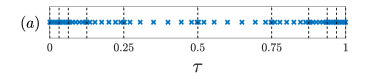
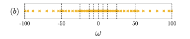
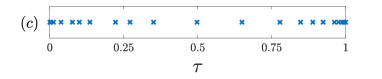
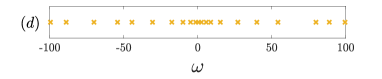
Figure 2: (a) Fine grid points $\tau_{i}^{f}$ for $p=8$ and $n=5$. Subinterval endpoints are indicated by the dashed lines. (b) Fine grid points $\omega_{k}^{f}$ for $p=8$ and $n=5$. (c) The $21$ imaginary time DLR nodes selected from the fine grid in (a) for $\Lambda=100$ and $\epsilon=10^{-6}$. For readability, we have used a smaller value of $p$ here than we do in practice. (d) The $21$ DLR frequencies selected from the fine grid in (b).

We refer to the nodes of this composite Chebyshev grid as the set of fine grid points in $\tau$, and denote them by $\{\tau_{j}^{f}\}_{j=1}^{M}$, using the single-index notation for a composite Chebyshev grid. Here, $M=p\times m$, where $m$ is the total number of subintervals in the partition of $[0,1]$. Thus we can ensure that for each fixed $\omega\in[-\Lambda,\Lambda]$, the composite Chebyshev interpolant on the fine grid in $\tau$ is uniformly accurate to $\epsilon_{\mbox{\tiny mach}}$; using the notation defined in Section III.1, we have

$$\norm{K(\tau,\omega)-\sum_{i=1}^{M}\overline{\ell}_{i}(\tau)K(\tau_{i}^{f},\omega)}_{\infty}<\epsilon_{\mbox{\tiny mach}}$$ (12)

with $M=\mathcal{O}\left(\log\Lambda\right)$.

We next consider fixed $\tau_{0}\in[0,1]$, for which we have $K(\tau_{0},\omega)=e^{-\tau_{0}\omega}/\left(1+e^{-\omega}\right)$. This is again a family of functions which are sharply peaked near the origin, and we discretize $[-\Lambda,\Lambda]$ by a composite Chebyshev grid with intervals dyadically refined towards the origin from the positive and negative direction until the smallest panels are of unit size, which again requires $n\sim\log_{2}\Lambda$. A similar choice of $p$ is again sufficient to obtain accuracy $\epsilon_{\mbox{\tiny mach}}$ for any $\Lambda$. An example of this grid is shown in Figure 2b.

The resulting fine grid points in $\omega$ are denoted by $\{\omega_{j}^{f}\}_{k=1}^{N}$, and give a composite Chebyshev interpolant of $K(\tau,\omega)$ on $\omega\in[-\Lambda,\Lambda]$ for each $\tau$ which is uniformly accurate to $\epsilon_{\mbox{\tiny mach}}$; that is

$$\norm{K(\tau,\omega)-\sum_{j=1}^{N}K(\tau,\omega_{j}^{f})\overline{\ell}_{j}(\omega)}_{\infty}<\epsilon_{\mbox{\tiny mach}}$$ (13)

with $N=\mathcal{O}\left(\log\Lambda\right)$. We note an abuse of notation: $\overline{\ell}_{i}(\tau)$ refers to the truncated Lagrange polynomials for the fine grid in $\tau$, whereas $\overline{\ell}_{j}(\omega)$ refers to those for the fine grid in $\omega$. Combining (12) and (13), and possibly increasing $p$, we obtain

$$\norm{K(\tau,\omega)-\sum_{i=1}^{M}\sum_{j=1}^{N}\overline{\ell}_{i}(\tau)K(\tau_{i}^{f},\omega_{j}^{f})\overline{\ell}_{j}(\omega)}_{\infty}<\epsilon_{\mbox{\tiny mach}}.$$ (14)

We summarize as follows. The kernel $K(\tau,\omega)$ may be represented by composite Chebyshev interpolants of $M$ and $N$ terms in $\tau$ and $\omega$, respectively, with subintervals chosen by dyadically subdivision. These representations can be constructed at a negligible cost, and directly checked for accuracy. We have $M=pm$ and $N=pn$; in practice, we find $m=n=\max\left(\log_{2}\Lambda,1\right)$ and $p=24$ to be sufficient to ensure double precision machine accuracy.

For simplicity of exposition, we will assume in the remainder of the article that the interpolation errors in (12), (13), and (14) are identically zero. Indeed, given these estimates, $K(\tau,\omega)$ is indistinguishable from its interpolants to the machine precision, and we can just as well take the interpolants as our definition of $K$.

IV.2 The DLR basis

Define $A\in\mathbb{R}^{M\times N}$ with entries given by $A_{ij}=K(\tau_{i}^{f},\omega_{j}^{f})$. Figure 3a shows the singular values of $A$ for a few choices of $\Lambda$. Evidently, the singular values decay at least exponentially, so that for each fixed $\Lambda$, the $\epsilon$-rank of $A$ is $\mathcal{O}\left(\log(1/\epsilon)\right)$. Figure 3b shows that the rate of exponential decay is proportional to $\log(\Lambda)$. It follows that the $\epsilon$-rank is $\mathcal{O}\left(\log(\Lambda)\log(1/\epsilon)\right)$. A derivation and analysis of this bound will be given in a forthcoming publication. chen_inprep

Since the column space of $A$ characterizes the subspace of imaginary time Green’s functions defined by (3), the low numerical rank of $A$ shows that this subspace is finite-dimensional to a good approximation. An equivalent observation is made in Ref. shinaoka17, , where it justifies using the left singular vectors of a discretization of $K(\tau,\omega)$ as a compressed representation of imaginary time Green’s functions. This is the IR basis, which we discuss in detail in Section V.

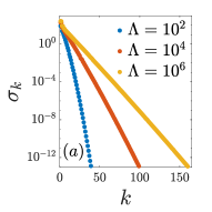
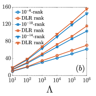
Figure 3: (a) Singular values $\sigma_{k}$ of the matrix $A_{ij}=K(\tau_{i}^{f},\omega_{j}^{f})$, for various $\Lambda$. (b) $\epsilon$-rank of $A$ against $\Lambda$ for various $\epsilon$ (blue), and the DLR rank (number of DLR basis functions) for the same choice of $\epsilon$ (orange).

Here, we use the ID to build a basis for the column space of $A$. Let $\epsilon$ be a user-provided error tolerance. We can construct a rank $r$ ID of $A$,

$$A=BP+E,$$ (15)

for $B\in\mathbb{R}^{M\times r}$, $P\in\mathbb{R}^{r\times N}$, and $E\in\mathbb{R}^{M\times N}$ an error matrix with

$$\norm{E}_{2}\leq\epsilon.$$

It follows from (9) and the rapid decay of the singular values of $A$ that $r$ will be at worst only slightly larger than the true $\epsilon$-rank of $A$. The discrepancy is shown in Figure 3b, with the blue points showing the true $\epsilon$-rank $r$ against $\Lambda$ for several $\epsilon$, and the orange points showing $r$ as obtained by the ID with the same choices of $\epsilon$, which we refer to as the DLR rank. This is a useful figure to refer to, as it shows the number of DLR basis functions required to represent any imaginary time Green’s function obeying a high energy cutoff $\Lambda$ to a given $\epsilon$ accuracy.

Writing (15) entrywise gives

$$K(\tau_{i}^{f},\omega_{j}^{f})=\sum_{l=1}^{r}K(\tau_{i}^{f},\omega_{l})P_{lj}+E_{ij}$$

for a subset $\{\omega_{l}\}_{l=1}^{r}$ of $\{\omega_{j}^{f}\}_{j=1}^{N}$. This subset corresponds to the selected columns in the ID, and we refer to it as the collection of DLR frequencies. Summing both sides against $\overline{\ell}_{i}(\tau)$ and $\overline{\ell}_{j}(\omega)$ gives

$$K(\tau,\omega)=\sum_{l=1}^{r}K(\tau,\omega_{l})\pi_{l}(\omega)+E(\tau,\omega)$$

with $\pi_{l}(\omega)=\sum_{j=1}^{n}P_{lj}\overline{\ell}_{j}(\omega)$ and $E(\tau,\omega)=\sum_{i=1}^{M}\sum_{j=1}^{N}\overline{\ell}_{i}(\tau)E_{ij}\overline{\ell}_{j}(\omega)$. Inserting this into (3), we obtain

$$\begin{multlined}G(\tau)=-\sum_{l=1}^{r}K(\tau,\omega_{l})\int_{-\Lambda}^{\Lambda}\pi_{l}(\omega)\rho(\omega)\,d\omega\\ -\int_{-\Lambda}^{\Lambda}E(\tau,\omega)\rho(\omega)\,d\omega.\end{multlined}G(\tau)=-\sum_{l=1}^{r}K(\tau,\omega_{l})\int_{-\Lambda}^{\Lambda}\pi_{l}(\omega)\rho(\omega)\,d\omega\\ -\int_{-\Lambda}^{\Lambda}E(\tau,\omega)\rho(\omega)\,d\omega.$$ (16)

Letting $\widehat{g}_{l}=-\int_{-\Lambda}^{\Lambda}\pi_{l}(\omega)\rho(\omega)\,d\omega$ gives our first main result. The bound on the error term is proven in Appendix B.

Theorem 1.

Suppose $G$ is given by its truncated Lehmann representation (3). Then there exist coefficients $\{\widehat{g}_{l}\}_{l=1}^{r}$ such that

$$G(\tau)=\sum_{l=1}^{r}K(\tau,\omega_{l})\widehat{g}_{l}+e(\tau)$$ (17)

with $\{\omega_{l}\}_{l=1}^{r}$ chosen corresponding to the selected columns of the ID (15). The error term $e(\tau)$ satisfies

$$\norm{e}_{\infty}\leq c\epsilon\norm{\rho}_{1}$$

for a constant $c$ which depends only on $p$, the Chebyshev degree parameter defined above.

The constant $c$ is mild and computable; for $p=24$, it is less than $10$. The $r$ functions $K(\tau,\omega_{l})$ are referred to as the DLR basis functions, and are characterized solely by the DLR frequencies $\omega_{l}$ selected in the ID. An example of a set of DLR frequencies, selected from the fine grid shown in Figure 2b with $\Lambda=100$ and $\epsilon=10^{-6}$, is shown in Figure 2d.

We note that in practice, it is not necessary to form the full ID in order to obtain the DLR basis, since we do not use the projection matrix $P$. Rather, we only need to identify the DLR frequencies $\{\omega_{l}\}_{l=1}^{r}$. The selection of the DLR frequencies takes place in the pivoted QR step of the ID algorithm. Thus to construct the DLR basis, we simply apply the rank-revealing pivoted QR algorithm to the columns of $A$ with a tolerance $\epsilon$.

IV.3 The imaginary time DLR grid

In general, the spectral density $\rho$ is not known a priori, so we cannot find the coefficients $\widehat{g}_{l}$ in (17) using the construction above. Rather, we will identify a set of $r$ imaginary time interpolation nodes $\tau_{k}$ so that expansion coefficients can be recovered from the values $g_{k}=G(\tau_{k})$ by solving an interpolation problem using the basis functions $K(\tau,\omega_{l})$.

Consider the matrix $B\in\mathbb{R}^{M\times r}$ introduced above, with entries $B_{il}=K(\tau_{i}^{f},\omega_{l})$. Forming the ID of $B^{T}$ gives

$$B=R\mathcal{K},$$ (18)

with $\mathcal{K}\in\mathbb{R}^{r\times r}$ consisting of selected rows of $B$, and $R\in\mathbb{R}^{M\times r}$ the associated projection matrix. The $r$ selected rows of $B$ correspond to a subset $\{\tau_{k}\}_{k=1}^{r}$ of the fine grid points $\{\tau_{i}^{f}\}_{i=1}^{M}$ in imaginary time, which we refer to as the imaginary time DLR grid. We have

$$\mathcal{K}_{kl}=K(\tau_{k},\omega_{l}).$$ (19)

Writing (18) entrywise and summing over the truncated Lagrange polynomials in $\tau$, we obtain

$$K(\tau,\omega_{l})=\sum_{k=1}^{r}\gamma_{k}(\tau)K(\tau_{k},\omega_{l})\equiv\sum_{k=1}^{r}\gamma_{k}(\tau)\mathcal{K}_{kl}$$ (20)

with $\gamma_{k}(\tau)=\sum_{i=1}^{M}\overline{\ell}_{i}(\tau)R_{ik}$. Equation (20) tells us that the DLR basis functions can be recovered from their values at the imaginary time DLR grid points. It will follow that a Green’s function can similarly be recovered from its values on this grid. An example of an imaginary time DLR grid, selected from the fine grid shown in Figure 2a with $\Lambda=100$ and $\epsilon=10^{-6}$, is shown in Figure 2c.

The recovery may be carried out in practice by computing the values $g_{k}=G(\tau_{k})$ for $k=1,\ldots,r$, solving the interpolation problem

$$g=\mathcal{K}\widehat{g}$$ (21)

for DLR coefficients $\widehat{g}_{k}$, and using

$$G_{\text{DLR}}(\tau)=\sum_{l=1}^{r}K(\tau,\omega_{l})\,\widehat{g}_{k}$$ (22)

as an approximation of $G$. Here, $g,\widehat{g}\in\mathbb{R}^{r}$. Although it is tempting to compare (22) with (17) and assume $G_{\text{DLR}}\approx G$ holds to high accuracy, this is not guaranteed a priori. Indeed, if the interpolation nodes $\tau_{k}$ were not selected carefully, this would not be the case. However, the following stability result, proven in Appendix C, leads to an accuracy guarantee.

Lemma 1.

Suppose $G_{\text{DLR}}$ and $H_{\text{DLR}}$ are given by

$$G_{\text{DLR}}(\tau)=\sum_{l=1}^{r}K(\tau,\omega_{l})\widehat{g}_{l}$$

and

$$H_{\text{DLR}}(\tau)=\sum_{l=1}^{r}K(\tau,\omega_{l})\widehat{h}_{l},$$

respectively, with $\{\omega_{l}\}_{l=1}^{r}$ chosen as above. Let $g,h\in\mathbb{R}^{r}$ be given by $g_{k}=G_{\text{DLR}}(\tau_{k})$, $h_{k}=H_{\text{DLR}}(\tau_{k})$, with $\{\tau_{k}\}_{k=1}^{r}$ the imaginary time DLR grid determined by the selected rows of the ID (18). Then

$$\norm{G_{\text{DLR}}-H_{\text{DLR}}}_{\infty}\leq\sqrt{2}\norm{R}_{2}\norm{g-h}_{2}.$$

The ID guarantees that $\norm{R}_{2}$ is controlled; in particular, we have the estimate (10). Since $M=\mathcal{O}\left(\log\Lambda\right)$ and $r$ is small, this factor in the estimate is small in practice. With Lemma 1 in hand, we consider the following practical question: if a Green’s function $G$ is sampled at the DLR grid points with some error, how accurate is the approximation $G_{\text{DLR}}$ given by (22), with the coefficients $\rho_{l}$ obtained by solving the interpolation problem (21)?

Theorem 2.

Let $G$ be a Green’s function given by a truncated Lehmann representation (3). Let $g\in\mathbb{R}^{r}$ be a vector of samples of $G$ at the imaginary time DLR grid points $\tau_{k}$, up to an error $\eta\in\mathbb{R}^{r}$: $g_{k}=G(\tau_{k})+\eta_{k}$. Suppose $\widehat{g}\in\mathbb{R}^{r}$ solves the corresponding interpolation problem (21) up to a residual error $\alpha$: $\mathcal{K}\widehat{g}-g=\alpha$, with $\alpha\in\mathbb{R}^{r}$. Let $G_{\text{DLR}}$ be given by

$$G_{\text{DLR}}(\tau)=\sum_{l=1}^{r}K(\tau,\omega_{l})\widehat{g}_{l}.$$

Then

$$\norm{G-G_{\text{DLR}}}_{\infty}\leq c\left(1+\sqrt{2r}\norm{R}_{2}\right)\norm{\rho}_{1}\epsilon\\ +\sqrt{2}\norm{R}_{2}\left(\norm{\eta}_{2}+\norm{\alpha}_{2}\right)$$

with $c$ the constant from Theorem 1.

Proof.

Theorem 1 guarantees that

$$G(\tau)=H_{\text{DLR}}(\tau)+e(\tau)$$

for $H_{\text{DLR}}$ a DLR expansion and $e$ a controlled error. We also have that

$$G_{\text{DLR}}(\tau_{k})=g_{k}+\alpha_{k}=G(\tau_{k})+\eta_{k}+\alpha_{k}.$$

These expressions, and Lemma 1, give

$$\norm{G-G_{\text{DLR}}}_{\infty} =\norm{e+H_{\text{DLR}}-G_{\text{DLR}}}_{\infty}$$

$$\leq\norm{e}_{\infty}+\sqrt{2}\norm{R}_{2}\norm{\{e(\tau_{k})\}_{k=1}^{r}+\eta+\alpha}_{2}$$

$$\begin{multlined}\leq\left(1+\sqrt{2r}\norm{R}_{2}\right)\norm{e}_{\infty}\\ +\sqrt{2}\norm{R}_{2}\left(\norm{\eta}_{2}+\norm{\alpha}_{2}\right).\end{multlined}\leq\left(1+\sqrt{2r}\norm{R}_{2}\right)\norm{e}_{\infty}\\ +\sqrt{2}\norm{R}_{2}\left(\norm{\eta}_{2}+\norm{\alpha}_{2}\right).$$

The result follows from the bound on $\norm{e}_{\infty}$ given in Theorem 1. ∎

It is expected, and our numerical experiments confirm, that typically $\norm{\alpha}_{2}\approx\norm{\eta}_{2}$. Thus the accuracy of the approximation (22) is indeed determined by the user-input error tolerance $\epsilon$, and is limited only by the accuracy to which $G$ can be evaluated. We remark that this holds true despite the fact that the matrix $\mathcal{K}$ is ill-conditioned, and therefore that the computed DLR coefficients $\widehat{g}_{l}$ are not expected to be close to those appearing in (17). Indeed, this ill-conditioning reflects a fundamental non-uniqueness in $\widehat{g}_{l}$. However, it will not prevent a standard linear solver from identifying a solution with small residual, and therefore does not imply any difficulty in accurately representing $G$.

IV.4 DLR in the Matsubara frequency domain

A DLR can be transformed to the Matsubara frequency domain analytically. Indeed, we have

$$K(i\nu_{n},\omega)=\int_{0}^{1}K(\tau,\omega)e^{-i\nu_{n}\tau}d\tau=\left(\omega+i\nu_{n}\right)^{-1},$$ (23)

with Matsubara frequency points

$$i\nu_{n}=\begin{cases}i(2n+1)\pi&\text{for fermionic Green's functions}\\ i2n\pi&\text{for bosonic Green's functions.}\end{cases}$$

A DLR expansion $G(\tau)=\sum_{l=1}^{r}K(\tau,\omega_{l})\widehat{g}_{l}$ therefore transforms to the Matsubara frequency domain as

$$G(i\nu_{n})=\sum_{l=1}^{r}K(i\nu_{n},\omega_{l})\widehat{g}_{l}.$$

We can construct a set of Matsubara frequency interpolation nodes using the ID. As in the previous section, we simply apply the ID to the rows of the matrix with entries $K(i\nu_{n},\omega_{l})$, for $n=-n_{\max},\ldots,n_{\max}$, and $l=1,\ldots,r$. Here $n_{\max}$ is a chosen Matsubara frequency cutoff. This process returns $r$ selected Matsubara frequency interpolation nodes $i\nu_{n_{k}}$. As before, it is not necessary to form the full ID, but only to use the pivoted QR algorithm to identify the selected nodes. The DLR coefficients can be recovered by solving the interpolation problem

$$G(i\nu_{n_{k}})=\sum_{l=1}^{r}K(i\nu_{n_{k}},\omega_{l})\widehat{g}_{l},$$ (24)

for $k=1,\ldots,r$, which is analogous to (21). One must ensure that the Matsubara frequency nodes have been converged with respect to $n_{\max}$, and in practice we find $n_{\max}\sim\Lambda$ is usually a sufficient cutoff.

This procedure requires carrying out the pivoted QR algorithm on the rows of a $2n_{\max}+1\times r$ matrix, and typically $n_{\max}=\mathcal{O}\left(\Lambda\right)$. It is more expensive than the procedure to select the imaginary time DLR grid points, which uses the pivoted QR algorithm on an $M\times r$ matrix, with $M=\mathcal{O}\left(\log\Lambda\right)$. However, it is still quite fast in practice for moderate values of $\Lambda$. If it were to become a bottleneck, one could design a more efficient scheme to select the Matsubara frequency interpolation nodes from a smaller subset of the full Matsubara frequency grid $-n_{\max}\leq n\leq n_{\max}$.

IV.5 Summary of DLR algorithms

We pause to summarize the practical procedures we have described to build and work with the DLR.

Construction of the DLR basis

To construct the DLR basis for a given choice of $\Lambda$ and $\epsilon$, we first discretize the kernel $K(\tau,\omega)$ on a composite Chebyshev grid to obtain the matrix with entries $A_{ij}=K(\tau_{i}^{f},\omega_{j}^{f})$. We then apply the pivoted QR algorithm, with an error tolerance $\epsilon$, to the columns of $A$. The pivots correspond to a set of $r$ DLR frequencies $\omega_{l}$, where $r$, the so-called DLR rank, is the number of basis functions required to represent the full subspace characterized by the truncated Lehmann integral operator to an accuracy approximately $\epsilon$. The DLR basis functions are simply given by $\{K(\tau,\omega_{l})\}_{l=1}^{r}$.

DLR from imaginary time values

To obtain the $r$ imaginary time interpolation nodes $\tau_{k}$, we simply apply the pivoted QR algorithm to the rows of the matrix with entries $B_{il}=K(\tau_{i}^{f},\omega_{l})$. The pivots correspond to the interpolation nodes. To obtain the DLR coefficients $\widehat{g}_{l}$ of a Green’s function $G(\tau)$, we compute the $r$ values $g_{k}=G(\tau_{k})$ and solve the $r\times r$ interpolation problem (21).

DLR from Matsubara frequency values

To obtain the $r$ Matsubara frequency interpolation nodes $i\nu_{n_{k}}$, we apply the pivoted QR algorithm in the same manner to the rows of the matrix with entries $K(i\nu_{n},\omega_{l})$, where $-n_{\max}\leq n\leq n_{\max}$ for some choice of $n_{\max}$. In practice, we find $n_{\max}=\Lambda$ to be sufficient in most cases, but $n_{\max}$ can be increased until the selected Matsubara frequency nodes no longer change. To obtain the DLR expansion coefficients $\widehat{g}_{l}$ of a Green’s function $G(i\nu_{n})$ in the Matsubara frequency domain, we solve the interpolation problem (24).

Transforming between imaginary time and Matsubara frequency domains

The DLR coefficients for the representation of a given Green’s function in the imaginary time and Matsubara frequency domains are the same; one simply takes the Fourier transform of the DLR in imaginary time explicitly using (23) to obtain the DLR in Matsubara frequency, and inverts the transform explicitly to go in the opposite direction. Thus, having obtained DLR coefficients for a Green’s function, the representation can be evaluated in either domain.

A remark on the selection of $\Lambda$ and $\epsilon$

In our framework, both $\Lambda$ and $\epsilon$ are user-determined parameters which control the accuracy of a given representation, and each choice of $\Lambda$ and $\epsilon$ yields some basis of $r$ functions which should then all be used. This is different from many typical methods, like orthogonal polynomial approximation, in which one simply converges a given calculation with respect to the number $m$ of basis functions directly. The inclusion of such a user-determined accuracy parameter $\epsilon$ is a desirable feature of many modern algorithms used in scientific computing, which enables automatic data compression with an accuracy guarantee.

In practice, to obtain a desired accuracy with the smallest possible number of basis functions, one should choose $\epsilon$ according to that desired accuracy, and not smaller. One should then converge with respect to $\Lambda$, which describes the frequency content of the problem, and is therefore more analogous to the parameter $m$ in the Legendre polynomial method. This process is illustrated, for example, by Figure 4, which is discussed in the next subsection.

IV.6 Numerical examples

We can test the algorithms described above by evaluating a known Green’s function on the imaginary time or Matsubara frequency DLR grids, recovering the corresponding DLR coefficients, and measuring the accuracy of the resulting DLR expansion by computing its error against $G(\tau)$. We use fermionic Green’s functions for all examples.

We first test the imaginary time sampling approach using the Green’s function corresponding to the spectral density $\rho(\omega)=\frac{2}{\pi}\sqrt{1-\omega^{2}}\theta\left(1-\omega^{2}\right)$. We fix $\epsilon$, and measure the $L^{\infty}$ error of the computed DLR for several choices of $\Lambda$. Results for $\beta=10^{4}$ were already presented in Figure 1c, in which we plot error against the number $r$ of basis functions obtained using $\Lambda=0.2\times 10^{4},0.4\times 10^{4},\ldots,1.2\times 10^{4}$, for $\epsilon=10^{-6}$, $10^{-10}$, and $10^{-14}$. We observe rapid convergence with $r$ to error $\epsilon$ in each case.

In Figures 4 and 5, respectively, we present similar plots for $\beta=10^{2}$ and $\beta=10^{6}$. In Figures 4c and 5c, we plot the error against $\Lambda$ directly. These plots demonstrate the method as it is used in practice; $\epsilon$ and $\Lambda$, not $r$, are chosen directly by the user in our framework. It can be seen from Figures 4b and 5b that choosing $\epsilon$ to be smaller than the actual desired accuracy simply yields a larger basis than is needed, as was discussed in Section IV.5 e.

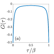
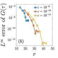
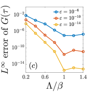
Figure 4: $L^{\infty}$ error of the DLR approximation of $G(\tau)=-\frac{2}{\pi}\int_{-1}^{1}K(\tau,\omega)\sqrt{1-\omega^{2}}\,d\omega$ obtained using imaginary time sampling for $\beta=10^{2}$ and several choices of $\epsilon$. (a) $G(\tau)$. (b) Error versus $r$, the number of basis functions. (c) Error versus $\Lambda$.

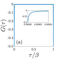
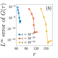
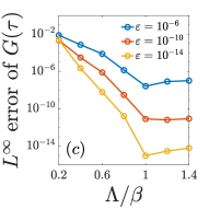
Figure 5: The same as in Figure 4, with $\beta=10^{6}$.

We next repeat the experiment using $\rho(\omega)=\left(\delta(-1/3)+\delta(1)\right)/2$ for $\beta=100$. The Green’s function is shown in Figure 6a, and the error versus $r$ in Figure 6b. The results are similar to those for the previous example. We note that the same experiments with $\beta=10^{4}$ and $\beta=10^{6}$, and $\Lambda$ adjusted accordingly, give the expected results.

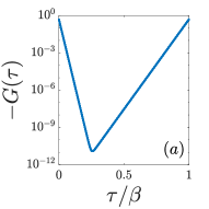
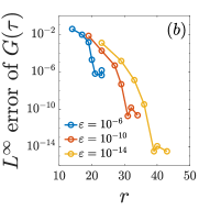
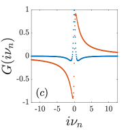
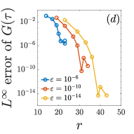
Figure 6: $L^{\infty}$ error of the DLR approximation of $G(\tau)=-\frac{1}{2}\int_{-1}^{1}K(\tau,\omega)\left(\delta(-1/3)+\delta(1)\right)\,d\omega$ for $\beta=100$ and several choices of $\epsilon$. (a) $G(\tau)$. (b) Error versus $r$ for imaginary time sampling. (c) $G(i\nu_{n})$; real part in blue, and imaginary part in orange. (d) Error versus $r$ for Matsubara frequency sampling.

To test the Matsubara frequency sampling approach, we repeat the same experiments, except that we recover the DLR coefficients from samples of the Green’s function on the Matsubara frequency DLR grid. As before, we measure the error in the imaginary time domain. Results for $\rho(\omega)=\frac{2}{\pi}\sqrt{1-\omega^{2}}\theta\left(1-\omega^{2}\right)$ with $\beta=10^{4}$ are shown in Figure 7. These can compared with Figure 1c. We observe only a mild loss of accuracy compared with the results obtained using imaginary time sampling, and we still achieve accuracy near $\epsilon$ when $\Lambda$ is increased beyond the known cutoff. Results for $\rho(\omega)=\left(\delta(-1/3)+\delta(1)\right)/2$ with $\beta=100$ are shown in Figures 6c and 6d. We have tested other choices of $\beta$ for both examples, up to $\beta=10^{6}$, with similar results.

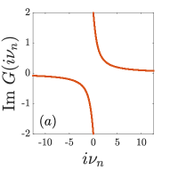
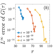
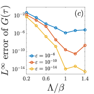
Figure 7: $L^{\infty}$ error of the DLR approximation of $G(\tau)=-\frac{2}{\pi}\int_{-1}^{1}K(\tau,\omega)\sqrt{1-\omega^{2}}\,d\omega$ obtained using Matsubara frequency sampling for $\beta=10^{4}$ and several choices of $\epsilon$. (a) $\operatorname{Im}G(i\nu_{n})$; note that $\operatorname{Re}G(i\nu_{n})=0$ by symmetry. (b) Error versus $r$. (c) Error versus $\Lambda$.

V Intermediate representation

In this section, we rederive the intermediate representation (IR) presented in Ref. shinaoka17, using the tools we have introduced to construct the DLR. The IR uses an orthonormal basis obtained from the SVD of an appropriate discretization of the kernel $K(\tau,\omega)$. It represents the same space as DLR, but has the advantage of orthogonality, at the cost of using more complicated basis functions. Our presentation of the IR differs from Refs. shinaoka17, ; chikano18, ; chikano19, ; shinaoka21_2, in two ways.

First, we show that discretizing $K$ on a composite grid like that introduced in Section IV.1 leads to an efficient construction of the IR basis. By contrast, in Ref. chikano18, , an automatic adaptive algorithm is used. The authors report in Ref. chikano19, that this algorithm takes on the order of hours to build the IR basis for $\Lambda=10^{4}$. To address this problem, the library irbasis contains precomputed basis functions for several values of $\Lambda$, and codes to work with them. chikano19 While this is a sufficient solution for many cases, it may be restrictive in others, for example in converging the IR with respect to $\Lambda$, or selecting $\Lambda$ to achieve a given accuracy with the smallest possible number of basis functions. Our approach, presented in Section V.1, does not require an expensive automatic adaptive algorithm. The IR basis is obtained by discretizing $K$ on a well-chosen grid, as before, and computing a single SVD of a matrix whose dimension grows logarithmically with $\Lambda$, and for $\Lambda$ up to $10^{6}$ is less than $1000$. As an illustration, Figure 8 contains plots of a few IR and DLR basis functions for $\Lambda=10^{4}$ and $\epsilon=10^{-14}$. Building each basis takes less than a second, despite the high resolution required.

Second, we show in Section V.2 that the interpolative decomposition of a matrix containing the $r$ IR basis functions naturally yields a set of $r$ sampling nodes for the IR, analogous to the interpolation grid for the DLR, and a transformation from values of a Green’s function at these nodes to its IR coefficients. In previous works, the sparse sampling method was used to provide such a sampling grid for the IR. li20 The sparse sampling nodes are chosen based on a heuristic, which is motivated by the relationship between orthogonal polynomials and their associated interpolation grids. While this heuristic appears to lead to a numerically stable algorithm, the procedure we have used to construct the DLR and Matsubara frequency grids is automatic and offers robust accuracy guarantees.

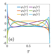
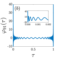
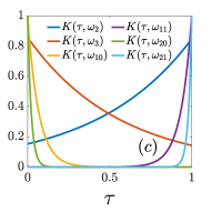
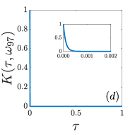
Figure 8: IR and DLR basis functions for $\Lambda=10^{4}$ and $\epsilon=10^{-14}$. (a) The first five IR basis functions. (b) The highest-degree (91st) IR basis function for the given parameters. (c) Several DLR basis functions for smaller $\omega_{l}$; we have ordered $\omega_{l}$ so that increasing $l$ corresponds to larger exponential rates. (d) The DLR basis function (96th) with the largest exponential decay rate for the given parameters.

V.1 The IR basis

The first step in constructing the IR basis is again to finely discretize $K(\tau,\omega)$. Here, to ensure that we obtain a basis which is orthogonal in the $L^{2}$ inner product, we use composite Legendre grids rather than composite Chebyshev grids. The discussion in Section IV.1 holds equally well for composite Legendre grids, with Gauss-Legendre nodes used in place of Chebyshev nodes.

In particular, let $\{\tau_{i}^{f}\}_{i=1}^{M}$ and $\{\omega_{j}^{f}\}_{j=1}^{N}$ be the nodes of the composite Legendre fine grids in $\tau$ and $\omega$, respectively, and let $A\in\mathbb{R}^{M\times N}$ be the matrix with entries $A_{ij}=K(\tau_{i}^{f},\omega_{j}^{f})$. Let $W\in\mathbb{R}^{M\times M}$ be a diagonal matrix with entries $W_{ii}=w_{i}^{f}$, the quadrature weights associated with the composite Legendre grid points $\tau_{i}^{f}$. The quadrature weights $\{w_{i}^{f}\}_{i=1}^{M}$ are obtained from the ordinary Gauss-Legendre quadrature weights at $p$ Legendre nodes, rescaled to account for the panel length.

Consider the SVD $\sqrt{W}A=U\Sigma V^{T}$ of the reweighted matrix. Truncating the SVD at rank $r$ gives

$$\sqrt{w_{i}^{f}}K(\tau_{i}^{f},\omega_{j}^{f})=\sum_{l=1}^{r}\sigma_{l}(u_{l})_{i}(v_{l})_{j}+E_{ij}$$

where $\sigma_{l}$, $\{u_{l}\}_{l=1}^{r}$, and $\{v_{l}\}_{l=1}^{r}$ are the first $r$ singular values, left singular vectors, and right singular vectors, respectively, and $E$ is an error matrix. As before, we choose $r$ so that $\norm{E}_{2}<\epsilon$, implying $r$ is the $\epsilon$-rank of $\sqrt{W}A$.

Note that the entries of each left singular vector $u_{l}$ can be interpreted as samples of a function on the fine grid in $\tau$, and similarly, the entries of $v_{l}$ as samples of a function on the fine grid in $\omega$. Summing against the corresponding truncated Lagrange polynomials, we find

$$K(\tau,\omega)=\sum_{l=1}^{r}\sigma_{l}\left(\sum_{i=1}^{M}\overline{\ell}_{i}(\tau)\frac{(u_{l})_{i}}{\sqrt{w_{i}^{f}}}\right)\left(\sum_{j=1}^{N}\overline{\ell}_{j}(\omega)(v_{l})_{j}\right)\\ +E(\tau,\omega),$$

with $E(\tau,\omega)=\sum_{i=1}^{M}\sum_{j=1}^{N}\frac{\overline{\ell}_{i}(\tau)}{\sqrt{w_{i}^{f}}}E_{ij}\overline{\ell}_{j}(\omega)$. Inserting this into the truncated Lehmann representation (3), we obtain

$$G(\tau)=-\sum_{l=1}^{r}\sigma_{l}\left(\sum_{i=1}^{M}\overline{\ell}_{i}(\tau)\frac{(u_{l})_{i}}{\sqrt{w_{i}^{f}}}\right)\\ \times\int_{-\Lambda}^{\Lambda}\left(\sum_{j=1}^{N}\overline{\ell}_{j}(\omega)(v_{l})_{j}\right)\rho(\omega)\,d\omega\\ -\int_{-\Lambda}^{\Lambda}E(\tau,\omega)\rho(\omega)\,d\omega.$$

This establishes the validity of the representation

$$G(\tau)=\sum_{l=1}^{r}\widehat{g}_{l}\varphi_{l}(\tau)+e(\tau)$$

for

$$\varphi_{l}(\tau)=\sum_{i=1}^{M}\overline{\ell}_{i}(\tau)\frac{(u_{l})_{i}}{\sqrt{w_{i}^{f}}},$$

and $e(\tau)$ an error term, analogous to the result in Theorem 1. We do not give an explicit bound on $e(\tau)$ here, but evidently it is similar to that for the DLR case.

The orthonormality of the collection $\{\varphi_{l}\}_{l=1}^{r}$ follows from that of the left singular vectors $\{u_{l}\}_{l=1}^{r}$:

$$\begin{split}\int_{0}^{1}\varphi_{k}(\tau)\varphi_{l}(\tau)\,d\tau&=\sum_{i=1}^{M}\varphi_{k}(\tau_{i}^{f})\varphi_{l}(\tau_{i}^{f})w_{i}^{f}\\ &=\sum_{i=1}^{M}(u_{k})_{i}(u_{l})_{i}=\delta_{kl}.\end{split}$$ (25)

Here, the first equality holds because the functions $\{\varphi_{l}\}_{l=1}^{r}$ are piecewise polynomials of degree $p-1$, so the Gauss-Legendre quadrature rule is exact, and the second follows from the definition of $\varphi_{l}$ and the truncated Lagrange polynomials. We define the IR basis as $\{\varphi_{l}\}_{l=1}^{r}$.

The functions $\varphi_{l}$ are represented using the singular vectors $\{u_{l}\}_{l=1}^{r}$ of $\sqrt{W}A$, so constructing them only requires forming and computing the SVD of this $M\times N$ matrix, with $M,N=\mathcal{O}\left(\log\Lambda\right)$, truncated to include only singular values larger than some desired accuracy $\epsilon$.

Operations involving the IR basis functions are straightforwardly carried out by working with the piecewise polynomial representation. For example, to evaluate $\varphi_{l}$ at a point $\tau$, we first find the subinterval in the composite Legendre grid containing $\tau$, and then evaluate a Legendre expansion on that subinterval at $\tau$. It follows from the orthonormality of the IR basis, and the exactness of Gauss-Legendre quadrature on polynomials of degree $2p-1$, that the IR coefficients of a Green’s function

$$G(\tau)=\sum_{l=1}^{r}\widehat{g}_{l}\varphi_{l}(\tau)$$ (26)

are given by

$$\begin{split}\widehat{g}_{l}&=\int_{0}^{1}\varphi_{l}(\tau)G(\tau)\,d\tau\\ &=\sum_{i=1}^{M}\varphi_{l}(\tau_{i}^{f})G(\tau_{i}^{f})w_{i}^{f}=\sum_{i=1}^{M}(u_{l})_{i}\,G(\tau_{i}^{f})\,\sqrt{w_{i}^{f}}.\end{split}$$ (27)

V.2 The imaginary time IR grid and transform matrix

Computing the IR coefficients using (27) requires sampling $G(\tau)$ at $M\gg r$ grid points. As for the imaginary time DLR grid, we show how to obtain $r$ imaginary time IR grid points $\{\tau_{i}\}_{i=1}^{r}$ and an $r\times r$ transform matrix $T$ so that given a Green’s function (26), we have $\widehat{g}_{l}\approx\sum_{k=1}^{r}T_{lk}\,G(\tau_{k})$ to high accuracy. We note that since the IR basis is orthogonal, it is natural to use projection rather than interpolation to obtain the expansion coefficients, so the procedure here is different than that for the DLR basis.

Let $\Phi$ be the matrix containing the IR basis functions on the fine grid, $\Phi_{ij}=\varphi_{j}(\tau_{i}^{f})=(u_{j})_{i}/\sqrt{w_{i}^{f}}$. The ID of $\Phi^{T}$ gives

$$\Phi=R\phi$$

with $\phi\in\mathbb{R}^{r\times r}$ consisting of selected rows of $\Phi$, and $R\in\mathbb{R}^{M\times r}$ the projection matrix. We take $\{\tau_{k}\}_{k=1}^{r}$ to be the subset of the fine grid points $\{\tau_{i}^{f}\}_{i=1}^{M}$ corresponding to the selected rows of $\Phi$, and define an $r\times r$ matrix

$$T=\Phi^{T}WR.$$ (28)

Suppose $G$ is given by (26), and let $g,\widehat{g}\in\mathbb{R}^{r}$ with $g_{k}=G(\tau_{k})$. In particular, we have $\phi\widehat{g}=g$. Then

$$Tg=\Phi^{T}WRg=\Phi^{T}WR\phi\widehat{g}=\Phi^{T}W\Phi\widehat{g}=\widehat{g}$$

since $\Phi^{T}W\Phi=I$ from (25). Thus, the imaginary time IR grid points and transform matrix can be computed directly from the ID of $\Phi$, and can be used to recover the IR coefficients from the values of a Green’s function on the IR grid.

We note that since the IR basis is orthogonal, issues of stability are more straightforward than in the DLR case, and we do not give a detailed analysis here.

V.3 IR in the Matsubara frequency domain

One can construct a Matsubara frequency grid for the IR basis using similar techniques to those presented in Section IV.4. In this case, however, we do not have simple analytical expressions for the Fourier transforms of the IR basis functions, and these have to be computed by numerical integration using the piecewise polynomial representations. This process is cumbersome compared with the analogous method for the DLR basis, and we will not describe it in detail.

As an alternative, to recover the IR coefficients from samples of a Green’s function in the Matsubara frequency domain, one could simply evaluate the Green’s function on the Matsubara frequency DLR grid, recover the DLR coefficients, evaluate the resulting DLR expansion on the IR grid, and apply the transform $T$.

VI Dyson equation in the DLR basis

We consider the Dyson equation relating a Matsubara Green’s function and self-energy,

$$G^{-1}(i\nu_{n})=G^{-1}_{0}(i\nu_{n})-\Sigma(i\nu_{n}),$$ (29)

where $G_{0}$ is a given Matsubara Green’s function. Although it is diagonal in the Matsubara frequency domain, it can also be written in the time domain as an integral equation,

$$G(\tau)-\int_{0}^{\beta}d\tau^{\prime}G_{0}(\tau-\tau^{\prime})\int_{0}^{\beta}d\tau^{\prime\prime}\Sigma(\tau^{\prime}-\tau^{\prime\prime})G(\tau^{\prime\prime})=G_{0}(\tau).$$ (30)

The functions $G$, $G_{0}$, and $\Sigma$ can be extended to $(-\beta,0)$ using the $\beta$-antiperiodicity property $f(-\tau)=-f(\beta-\tau)$ or the $\beta$-periodicity property $f(-\tau)=f(\beta-\tau)$ for fermionic and bosonic Green’s functions, respectively. Since $G(\tau)$ is an imaginary time Green’s function, it has a Lehmann spectral representation (1), and can therefore be approximated by a DLR. We assume the same is true of the self-energy $\Sigma$, and of the intermediate convolutions in (30); this can be shown in many typical cases of physical interest. For simplicity, we assume in this section that all quantities are fermionic, but our discussion is straightforwardly extended to the bosonic case.

Since $\Sigma$ in general depends on $G$, the Dyson equation must be solved self-consistently by nonlinear iteration: see for example (39) in the next section for the SYK self-energy. The standard method is to compute $\Sigma$ in the imaginary time domain, where it is typically simpler, and to solve the Dyson equation (29) in the Matsubara frequency domain where it is diagonal. This procedure can be carried out efficiently using the DLR: (i) given $G$ on the imaginary time DLR grid computed from a previous iterate, $\Sigma$ is computed on the imaginary time DLR grid; (ii) the DLR coefficients of $\Sigma$ are recovered; (iii) $\Sigma$ is evaluated on the Matsubara frequency grid; (iv) (29) is solved to obtain $G$ on the Matsubara frequency grid; (v) the DLR coefficients of $G$ are recovered; and (vi) $G$ is evaluated on the imaginary time DLR grid to prepare for the next iterate. Ref. li20, describes and demonstrates a similar procedure using the sparse sampling method for the IR.

In this section, we show how to solve the Dyson equation directly in imaginary time using the DLR basis. We note that much of the discussion holds equally well for the IR basis – or any other basis, including an orthogonal polynomial basis GullStrand_2020 – however, certain quantities which must be computed by numerical integration in that case are given analytically for the DLR basis. We will work with the integral form (30), and assume $\Sigma$ is given, as is the case within a single step of nonlinear iteration.

Let $G$ be a Green’s function given by a DLR

$$G(\tau)=\sum_{l=1}^{r}K(\tau,\omega_{l})\widehat{g}_{l}$$

and let $g_{k}=G(\tau_{k})$. We will use similar notation for other quantities. We define the convolution between $\Sigma$ and $G$ by

$$F(\tau)\equiv\int_{0}^{1}\Sigma(\tau-\tau^{\prime})G(\tau^{\prime})\,d\tau^{\prime}.$$ (31)

Let $\overline{\Sigma}\in\mathbb{R}^{r\times r}$ denote the matrix discretizing this convolution, so that

$$f=\overline{\Sigma}g$$ (32)

with $f_{k}=F(\tau_{k})$. $\overline{\Sigma}$ can be constructed by a linear transformation of the values $\sigma_{k}=\Sigma(\tau_{k})$; there is a tensor $\mathcal{C}_{ijk}$ with

$$\overline{\Sigma}_{ij}=\sum_{k=1}^{r}\mathcal{C}_{ijk}\sigma_{k}.$$ (33)

As we will see, it may be simpler to form $\overline{\Sigma}$ from its DLR coefficients $\widehat{\sigma}_{l}$, and there is a tensor $\widehat{\mathcal{C}}_{ijl}$ with

$$\overline{\Sigma}_{ij}=\sum_{l=1}^{r}\widehat{\mathcal{C}}_{ijl}\widehat{\sigma}_{l}.$$ (34)

Using this notation, the discretization of (30) in the DLR basis is given by

$$(I-\overline{G}_{0}\overline{\Sigma})g=g_{0},$$ (35)

where $\overline{G}_{0}$ can be obtained as in (33) or (34). This is simply an $r\times r$ linear system. Thus, given $\Sigma$, $\overline{\Sigma}$ can be obtained using (33) or (34), and then (35) can be solved to obtain $G$ on the imaginary time DLR grid. It remains only to discuss the construction of the tensors $\mathcal{C}$ and $\widehat{\mathcal{C}}$.

We begin by discretizing the convolution (31) on the imaginary time DLR grid:

$$f_{k} =F(\tau_{k})=\int_{0}^{1}\Sigma(\tau_{k}-\tau^{\prime})G(\tau^{\prime})d\tau^{\prime}$$

$$=\sum_{l=1}^{r}\left(\int_{0}^{1}\Sigma(\tau_{k}-\tau^{\prime})K(\tau^{\prime},\omega_{l})\,d\tau^{\prime}\right)\widehat{g}_{l}\equiv\sum_{l=1}^{r}\widehat{\Sigma}_{kl}\widehat{g}_{l}.$$

Here we have defined $\widehat{\Sigma}$ as the matrix of convolution by $\Sigma$, which takes the DLR coefficients $\widehat{g}_{l}$ to the values $f_{l}$ of the convolution at the imaginary time DLR grid points. Recall the matrix $\mathcal{K}$ defined by (19), which gives $g=\mathcal{K}\widehat{g}$. Precomposing $\widehat{\Sigma}$ with $\mathcal{K}^{-1}$, we obtain the matrix

$$\overline{\Sigma}=\widehat{\Sigma}\mathcal{K}^{-1}$$

yielding (32). We can define the matrix $\overline{G}_{0}$ of convolution by $G_{0}$ similarly.

To construct $\widehat{\Sigma}$, we take $\Sigma(\tau)=\sum_{k=1}^{r}K(\tau,\omega_{j})\widehat{\sigma}_{k}$ and write

$$\widehat{\Sigma}_{ij} =\int_{0}^{1}\Sigma(\tau_{i}-\tau^{\prime})K(\tau^{\prime},\omega_{j})\,d\tau^{\prime}$$ (36)

$$=\begin{multlined}\int_{0}^{\tau_{i}}\Sigma(\tau_{i}-\tau^{\prime})K(\tau^{\prime},\omega_{j})\,d\tau^{\prime}\\ -\int_{\tau_{i}}^{1}\Sigma(1+\tau_{i}-\tau^{\prime})K(\tau^{\prime},\omega_{j})\,d\tau^{\prime}\end{multlined}\int_{0}^{\tau_{i}}\Sigma(\tau_{i}-\tau^{\prime})K(\tau^{\prime},\omega_{j})\,d\tau^{\prime}\\ -\int_{\tau_{i}}^{1}\Sigma(1+\tau_{i}-\tau^{\prime})K(\tau^{\prime},\omega_{j})\,d\tau^{\prime}$$

$$=\begin{multlined}\sum_{k=1}^{r}\widehat{\sigma}_{k}\left(\int_{0}^{\tau_{i}}K(\tau_{i}-\tau^{\prime},\omega_{k})K(\tau^{\prime},\omega_{j})\,d\tau^{\prime}\right.\\ \left.-\int_{\tau_{i}}^{1}K(1+\tau_{i}-\tau^{\prime},\omega_{k})K(\tau^{\prime},\omega_{j})\,d\tau^{\prime}\right)\end{multlined}\sum_{k=1}^{r}\widehat{\sigma}_{k}\left(\int_{0}^{\tau_{i}}K(\tau_{i}-\tau^{\prime},\omega_{k})K(\tau^{\prime},\omega_{j})\,d\tau^{\prime}\right.\\ \left.-\int_{\tau_{i}}^{1}K(1+\tau_{i}-\tau^{\prime},\omega_{k})K(\tau^{\prime},\omega_{j})\,d\tau^{\prime}\right)$$

$$=\sum_{k=1}^{r}\widetilde{\mathcal{C}}_{ijk}\widehat{\sigma}_{k},$$

where we have used the antiperiodicity property. A straightforward calculation shows that $\widetilde{\mathcal{C}}_{ijk}$ is given explicitly by

$$\widetilde{\mathcal{C}}_{ijk}=\begin{cases}\frac{K(\tau_{i},\omega_{j})-K(\tau_{i},\omega_{k})}{\omega_{k}-\omega_{j}}&\text{if }j\neq k\\ \left(\tau_{i}-K(1,\omega_{j})\right)K(\tau_{i},\omega_{j})&\text{if }j=k.\end{cases}$$

The matrix $\overline{\Sigma}$ is then given by

$$\overline{\Sigma}_{ij}=\sum_{k=1}^{r}\widehat{\Sigma}_{ik}\mathcal{K}^{-1}_{kj}=\sum_{k,l=1}^{r}\widetilde{\mathcal{C}}_{ikl}\widehat{\sigma}_{l}\mathcal{K}^{-1}_{kj}.$$

Defining

$$\widehat{\mathcal{C}}_{ijl}\equiv\sum_{k=1}^{r}\widetilde{\mathcal{C}}_{ikl}\mathcal{K}^{-1}_{kj}$$ (37)

gives (34). We remark that in practice $\mathcal{K}^{-1}$ should be applied in a numerically stable manner, such as by LU factorization and back substitution, rather than formed explicitly.

Inserting $\widehat{\sigma}=\mathcal{K}^{-1}\sigma$ into (34), we obtain (33) with

$$\mathcal{C}_{ijk}\equiv\sum_{l=1}^{r}\widehat{\mathcal{C}}_{ijl}\mathcal{K}^{-1}_{lk}.$$ (38)

However, if this computation is not done carefully, rounding error will lead to a significant loss of precision. In order to maintain full double precision accuracy using (33), $\widetilde{\mathcal{C}}$ and $\mathcal{K}$ must be formed in quadruple precision. This is of course straightforward, since the entries of these arrays are given explicitly. Then, (37) and (38) must be computed in quadruple precision. Once $\mathcal{C}$ has been obtained, all subsequent calculations – in particular, (33) – can be carried out in double precision. Describing this phenomenon requires an analysis of floating point errors which is beyond this scope of this paper. Alternatively, one can simply obtain $\widehat{\sigma}$ from $\sigma$ first, and use (34) instead of (33); then no such issue arises, and all arrays may be formed using double precision arithmetic.

We make a brief remark on the computational complexity of solving the Dyson equation using the DLR. The more standard method, using (29), scales as $\mathcal{O}\left(r^{2}\right)$, due to the cost of transforming between the imaginary time and Matsubara frequency DLR grid representations of $G$ and $\Sigma$. The sparse sampling method is similar, and has roughly the same cost. li20 By contrast, the imaginary time domain method we have described scales as $\mathcal{O}\left(r^{3}\right)$, due to the cost of forming $\overline{\Sigma}$ (the system (35) can typically be solved at an $\mathcal{O}\left(r^{2}\right)$ cost using an iterative linear solver). Methods of reducing this cost may exist, and will be explored in the future. However, since $r$ is typically small, the discrepancy may or may not be significant in practice, and the pure imaginary time domain method may be more convenient or robust in certain applications.

VII Example: the SYK equation

To demonstrate the method described in the previous section, we consider the Sachdev-Ye-Kitaev (SYK) equations, given by SachdevYe93 ; gu20

$$\begin{cases}G^{-1}(i\nu_{n})=i\nu_{n}+\mu-\Sigma(i\nu_{n})\\ \Sigma(\tau)=J^{2}G^{2}(\tau)G(\beta-\tau),\end{cases}$$ (39)

where $\mu$ is the chemical potential, $J$ is a coupling constant, and $G$ is a fermionic Matsubara Green’s function. We fix $J=1$.

The SYK model exhibits remarkable properties, and is the subject of a large literature. chowdhury21 Here, our motivation is to illustrate the efficiency of the DLR approach in solving a nonlinear Dyson equation. In the $\beta\to\infty$ limit, it is known that solutions develop a $1/\sqrt{\omega}$ non-Fermi liquid singularity at low frequencies, or equivalently $1/\sqrt{\tau}$ decay at large imaginary times. SachdevYe93 The DLR expansion captures this behavior with excellent accuracy. Although guaranteed by our analysis, this result may appear counterintuitive, but there is in fact a significant literature on the approximation of functions with power law decay by sums of a small number of exponentials. beylkin05 ; beylkin10 ; zhang21

We solve (39) in the DLR basis using the imaginary time domain method described in Section VI. Nonlinear iteration is carried out using a weighted fixed point iteration

$$\Sigma^{(n+1)}=\Sigma[w\,G^{(n)}+(1-w)\,G^{(n-1)}],$$

with the weight $w$ chosen to ensure convergence. We terminate the iteration when the values of $G^{(n)}$ and $G^{(n-1)}$ on the imaginary time DLR grid match pointwise to within a fixed point tolerance $\epsilon_{\text{fp}}$.

We first solve (39) with $\mu=0$ and $\beta=10^{4}$, using $G(\tau)=-1/2$ as the initial guess for the weighted fixed point iteration. We take $\epsilon=10^{-14}$, $\Lambda=5\beta$, $\epsilon_{\textrm{fp}}=10^{-12}$, and $w=0.15$. The calculation involves systems of only $117$ degrees of freedom, and takes less than a second on a laptop. $G(\tau)$ is plotted in Figure 9a, along with the conformal asymptotic solution $G_{c}(\tau)$ given by PhysRevB.63.134406 ; gu20

$$G_{c}(\tau)=-\frac{\pi^{1/4}}{\sqrt{2\beta}}\left(\sin\left(\frac{\pi\tau}{\beta}\right)\right)^{-1/2}.$$ (40)

In Figure 9b, we plot the difference $G(\tau)-G_{c}(\tau)$ for $\tau\in[0,\beta/2]$. We observe the expected $\mathcal{O}\left(\tau^{-3/2}\right)$ asymptotic correction to (40). In Figure 9c, we plot the error of $G(\tau)$ as compared with a standard Legendre polynomial-based solver, GullStrand_2020 which operates according to the description in Section VI with the DLR basis and nodes replaced by a Legendre polynomial basis and Legendre nodes.

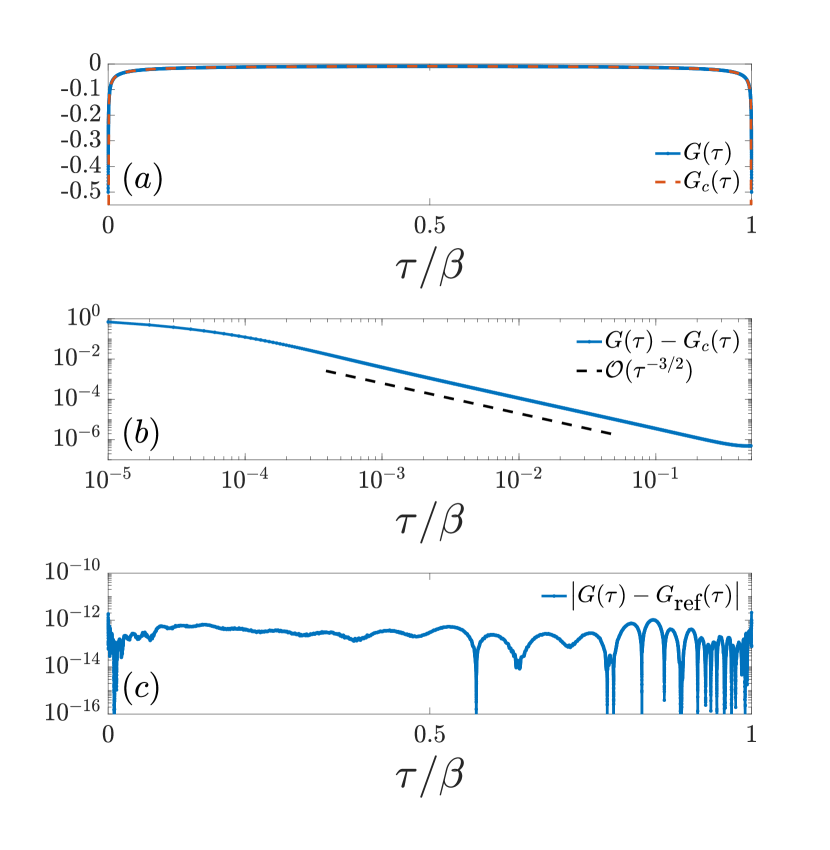
Figure 9: (a) Solution $G(\tau)$ of the SYK equation with $J=1$, $\mu=0$, and $\beta=10^{4}$, along with the conformal solution $G_{c}(\tau)$. (b) Pointwise difference $G-G_{c}$, showing the form of the higher-order correction. (c) Pointwise error of computed $G$ measured against a reference solution $G_{\text{ref}}$ obtained using Legendre polynomial-based solver.

We next carry out a high precision calculation of the compressibility in the SYK model in the zero temperature limit, following the results of Ref. gu20, (Sec. 4.2). We define the charge $Q$ (conventionally vanishing at half-filling) as

$$Q(\beta,\mu)\equiv(G_{\beta,\mu}(\beta)-G_{\beta,\mu}(0))/2,$$ (41)

where $G_{\beta,\mu}$ is the solution of (39) for fixed $\beta$ and $\mu>0$. The compressibility $K$ is defined as

$$K(T)=\left.\frac{\partial Q(\beta,\mu)}{\partial\mu}\right\rvert_{\mu=0^{+}}=\lim_{\mu\to 0^{+}}\frac{Q(\beta,\mu)}{\mu}$$ (42)

with $T=\beta^{-1}$.

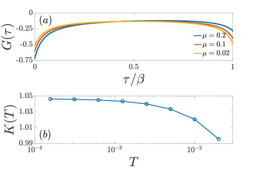
Figure 10: (a) Solution $G(\tau)$ of the SYK equation with $J=1$, $\beta=50$, and three values of $\mu$. (b) Compressibility $K(T)$ at low temperature.

Our goal is to calculate $K(0)=\lim_{T\to 0^{+}}K(T)$. $G(\beta,\mu)$ is shown for $\beta=50$ and $\mu=0.2,0.1,0.02$ in Figure 10a. As expected, $Q(\beta,\mu)$ is positive for $\mu>0$ and decreases to zero as $\mu\to 0$.

In order to calculate $K(T)$ for each fixed $T$, we could simply compute $Q(\beta,\mu)/\mu$ for a small value of $\mu$. However, this strategy suffers from rounding error due to catastrophic cancellation. To obtain a better approximation of $K(T)$, we compute $Q$ by solving the SYK equation for $\mu=\mu_{0}/2^{j}$, with $j=1,\ldots,n$, and some choice of $\mu_{0}$ and $n$. We then use Richardson extrapolation on the resulting values of $Q/\mu$ to obtain the limiting value $K(T)$; see Ref. dahlquist08, (Sec. 3.4.6) for a description of Richardson extrapolation.

We note that some care must be taken in the nonlinear iteration to avoid convergence to a spurious exponentially-decaying solution. An effective strategy is to compute the solution for a sequence of values of $\mu$: $\mu=j\mu^{*}/n$, $j=0,\ldots,n$, where $\mu^{*}$ is the desired value, and $n$ is chosen sufficiently large. For $\mu=0$, we use the initial guess $G(\tau)=-1/2$ in the nonlinear iteration, as above. For $\mu=j\mu^{*}/n$ with $j>0$, we use the solution for $\mu=(j-1)\mu^{*}/n$ as an initial guess. In many cases, taking $n=1$ is sufficient.

We carry out this procedure for $\beta=50,100,200,\ldots,6400$ with $\epsilon=10^{-14}$, $\epsilon_{\textrm{fp}}=10^{-12}$, and $w$ taken sufficiently small to ensure convergence of the nonlinear iteration. We take $\Lambda=10\beta$, and have verified that all calculations are converged with respect to this parameter. The computations involve linear systems of at most $121$ degrees of freedom.

The computed values of $K(T)$ are shown in Figure 10b. From these values, we use Richardson extrapolation to estimate $K(0)$:

$$K(0)\approx 1.0466998.$$

VIII Conclusion

We have presented an efficient discrete Lehmann representation of imaginary time Green’s functions based on the interpolative decomposition. In the low temperature regime, it requires far fewer degrees of freedom than standard discretizations, and a similar number to the recently introduced intermediate representation. The DLR basis functions are explicit; they are exponentials, carefully chosen to ensure stable and accurate approximation. This feature simplifies standard operations. We have introduced algorithms which use standard numerical linear algebra tools to efficiently build the DLR basis and corresponding imaginary time and Matsubara frequency grids. These algorithms also carry over to the intermediate representation method. We have demonstrated the DLR by solving the SYK equation to high precision at low temperatures, with calculations taking on the order of seconds on a laptop. Fortran and Python implementations of the algorithms described in this paper are available in the library libdlr. libdlr ; kaye21

Appendix A DLR for bosonic Green’s functions

In this section, we argue that the DLR, derived using the fermionic kernel $K(\tau,\omega)$ given by (2), can also be applied directly to bosonic Green’s functions.

The truncated Lehmann representation for a bosonic Green’s function is given by

$$G_{\text{B}}(\tau)=-\int_{-\Lambda}^{\Lambda}K_{\text{B}}(\tau,\omega)\rho_{\text{B}}(\omega)\,d\omega,$$ (43)

where the bosonic kernel is given in nondimensionalized variables by

$$K_{\text{B}}(\tau,\omega)=\frac{e^{-\omega\tau}}{1-e^{-\omega}}.$$ (44)

Although $K_{\text{B}}$ is singular at $\omega=0$, for systems in which the $U(1)$ symmetry $\left<\hat{a}\right>=0$ and $\left<\hat{a}^{\dagger}\right>=0$ (for $\hat{a}^{\dagger}$/$\hat{a}$ the creation/anniliation operators) is not spontaneously broken, the singularity will be exactly cancelled out by a spectral density vanishing to the appropriate order as $\omega\to 0$. Indeed, in this case, the physical spectral density of a bosonic system has an explicit expression,

$$\begin{multlined}\rho_{\text{B}}(\omega)=(1-e^{-\omega})\frac{2\pi}{Z}\\ \times\sum_{m,n}\left|\left<n|\hat{a}^{\dagger}|m\right>\right|^{2}e^{-E_{m}}\delta(E_{n}-E_{m}-\omega),\end{multlined}\rho_{\text{B}}(\omega)=(1-e^{-\omega})\frac{2\pi}{Z}\\ \times\sum_{m,n}\left|\left<n|\hat{a}^{\dagger}|m\right>\right|^{2}e^{-E_{m}}\delta(E_{n}-E_{m}-\omega),$$ (45)

where $\left|n\right>$ and $\left|m\right>$ are eigenstates of the many-body Hamiltonian with energies $E_{n}$ and $E_{m}$, respectively, and $Z=\sum_{n}e^{-E_{n}}$ is the partition sum.

To handle this case, we simply rewrite (43) as

$$G_{\text{B}}(\tau)=-\int_{-\Lambda}^{\Lambda}K(\tau,\omega)\widetilde{\rho_{\text{B}}}(\omega)\,d\omega,$$

where $K(\tau,\omega)$ is the fermionic kernel, and

$$\widetilde{\rho_{\text{B}}}(\omega)=\frac{1+e^{-\omega}}{1-e^{-\omega}}\rho_{\text{B}}(\omega).$$ (46)

The singularity in the factor $\frac{1+e^{-\omega}}{1-e^{-\omega}}$ is cancelled by the factor $1-e^{-\omega}$ in $\rho_{\text{B}}$ from (45); otherwise, it is smooth and well-behaved. Thus $\widetilde{\rho_{\text{B}}}$ is integrable, and $G_{\text{B}}$ has the same Lehmann representation as a fermionic Green’s function, but with a modified spectral density. The DLR method developed for fermionic Green’s functions can therefore be applied without modification.

Appendix B Proof of Theorem 1

• The theorem follows from (16), once we give a bound on the error term. We have

  $$\absolutevalue{e(\tau)} =\absolutevalue{\int_{-\Lambda}^{\Lambda}E(\tau,\omega)\rho(\omega)\,d\omega}$$

  $$=\absolutevalue{\sum_{i=1}^{M}\overline{\ell}_{i}(\tau)\sum_{j=1}^{N}E_{ij}\int_{-\Lambda}^{\Lambda}\overline{\ell}_{j}(\omega)\rho(\omega)\,d\omega}$$

  $$\leq\norm{E}_{2}\sqrt{\sum_{i=1}^{M}\overline{\ell}_{i}^{2}(\tau)}\sqrt{\sum_{j=1}^{N}\left(\int_{-\Lambda}^{\Lambda}\overline{\ell}_{j}(\omega)\rho(\omega)\,d\omega\right)^{2}}$$

  from the Cauchy-Schwarz inequality.

  From the definition of $\overline{\ell}_{i}$, we have $\norm{\sum_{i=1}^{M}\overline{\ell}_{i}^{2}(\tau)}_{\infty}=\norm{\sum_{k=1}^{p}\ell_{k}^{2}(x)}_{\infty}$, where $\ell_{k}(x)$ are the Lagrange polynomials at $p$ Chebyshev nodes on $[-1,1]$. It follows from Lemma 2, proven in Appendix D, that

  $$\sum_{k=1}^{p}\ell_{k}^{2}(x)\leq 2.$$

  For the last factor, we have

  $$\sum_{j=1}^{N}\left(\int_{-\Lambda}^{\Lambda}\overline{\ell}_{j}(\omega)\rho(\omega)\,d\omega\right)^{2}\leq\norm{\rho}_{1}^{2}\sum_{j=1}^{p}\left(\max_{x\in[-1,1]}\absolutevalue{\ell_{j}(x)}\right)^{2}.$$

  Combining these results, we find

  $$\norm{e}_{\infty}\leq\sqrt{2\sum_{j=1}^{p}\left(\max_{x\in[-1,1]}\absolutevalue{\ell_{j}(x)}\right)^{2}}\norm{E}_{2}\norm{\rho}_{1}=c\epsilon\norm{\rho}_{1}.$$

  We note that $\sum_{j=1}^{p}\left(\max_{x\in[-1,1]}\absolutevalue{\ell_{j}(x)}\right)^{2}$ depends only on $p$. Numerically, we find that it is approximately equal to $p$ for typical choices of $p$, implying $c\approx\sqrt{2p}.$ ∎

Appendix C Proof of Lemma 1

• From (20), we have

  $$G_{\text{DLR}}(\tau)=\sum_{l=1}^{r}\widehat{g}_{l}\sum_{k=1}^{r}\gamma_{k}(\tau)\mathcal{K}_{kl}=\sum_{k=1}^{r}\gamma_{k}(\tau)g_{k}$$

  and similarly for $H_{\text{DLR}}$, so

  $$G_{\text{DLR}}(\tau)-H_{\text{DLR}}(\tau)=\sum_{k=1}^{r}\gamma_{k}(\tau)\left(g_{k}-h_{k}\right)$$

  and

  $$\absolutevalue{G_{\text{DLR}}(\tau)-H_{\text{DLR}}(\tau)}\leq\sqrt{\sum_{k=1}^{r}\gamma_{k}^{2}(\tau)}\,\norm{g-h}_{2}.$$

  Since $\gamma_{k}(\tau)=\sum_{i=1}^{M}\overline{\ell}_{i}(\tau)R_{ik}$, we have

  $$\sum_{k=1}^{r}\gamma_{k}^{2}(\tau)\leq\norm{R}_{2}^{2}\sum_{i=1}^{M}\overline{\ell}_{i}^{2}(\tau)\leq 2\norm{R}_{2}^{2}.$$

  Here we have used Lemma 2 from Appendix D, as in Appendix B. The result follows from these estimates. ∎

Appendix D Bound on the sum of squares of Lagrange polynomials for Chebyshev nodes

The following lemma is used in Appendices B and C:

Lemma 2.

Let $\{\ell_{k}(x)\}_{k=1}^{p}$ be the Lagrange polynomials for the $p$ Chebyshev nodes of the first kind on $[-1,1]$. Then

$$\sum_{k=1}^{p}\ell_{k}^{2}(x)\leq\sum_{k=1}^{p}\ell_{k}^{2}(1)=2-1/p.$$

Proof.

The result follows from the identity

$$\sum_{k=1}^{p}\ell_{k}^{2}(x)=1+\frac{1}{2p}\left(U_{2p-2}(x)-1\right),$$ (47)

for $U_{n}(x)$ the degree $n$ Chebyshev polynomial of the second kind. Indeed, Ref. nistdlmf, (Eqn. 18.14.1) gives that

$$\absolutevalue{U_{n}(x)}\leq U_{n}(1)=n+1,$$

and the desired result follows from this and (47).

To prove (47), we note that both the left and right hand sides are polynomials of degree $2p-2$, so it suffices to show that they agree in value and derivative at the $p$ Chebyshev nodes,

$$x_{j}=\cos\left(\frac{2j-1}{2p}\pi\right),$$

for $j=1,\ldots,p$.

For the equality of values, the sine difference formula gives

$$U_{2p-2}(x_{j})=\frac{\sin\left((2p-1)\frac{2j-1}{2p}\pi\right)}{\sin\left(\frac{2j-1}{2p}\pi\right)}=1.$$

Since $\sum_{k=1}^{p}\ell_{k}^{2}(x_{j})=1$, this gives the equality.

For the equality of derivatives, we must show that

$$2\sum_{k=1}^{p}\ell_{k}(x)\ell_{k}^{\prime}(x)=\frac{1}{2p}U^{\prime}_{2p-2}(x)$$

for each $x=x_{j}$. Throughout the argument, we will use the formulas for the derivatives of the Chebyshev polynomials of the first and second kind, given by

$$T_{n}^{\prime}(x)=nU_{n-1}(x)$$

and

$$U_{n}^{\prime}(x)=\frac{(n+1)T_{n+1}(x)-xU_{n}(x)}{x^{2}-1}.$$

The cosine difference formula gives

$$\frac{U^{\prime}_{2p-2}(x_{j})}{2p} =\frac{(2p-1)T_{2p-1}(x_{j})-x_{j}U_{2p-2}(x_{j})}{2p\,(x_{j}^{2}-1)}$$

$$=\frac{(2p-1)\cos\left((2p-1)\frac{2j-1}{2p}\pi\right)-x_{j}}{2p\,(x_{j}^{2}-1)}$$

$$=\frac{x_{j}}{1-x_{j}^{2}}$$

for the right hand side. For the left hand side, we have

$$2\sum_{k=1}^{p}\ell_{k}(x_{j})\ell_{k}^{\prime}(x_{j})=2\ell_{j}^{\prime}(x_{j})=\sum_{\begin{subarray}{c}k=0\\ k\neq j\end{subarray}}^{p}\frac{2}{x_{j}-x_{k}}.$$

Our objective is therefore to show that

$$\sum_{\begin{subarray}{c}k=0\\ k\neq j\end{subarray}}^{p}\frac{2}{x_{j}-x_{k}}=\frac{x_{j}}{1-x_{j}^{2}}$$ (48)

for $j=1,\ldots,p$.

Define

$$f_{j}(x)=\sum_{\begin{subarray}{c}k=0\\ k\neq j\end{subarray}}^{p}\frac{1}{x-x_{k}},$$

so that the left hand side of (48) is equal to $f_{j}(x_{j})$. Let $\ell(x)=\prod_{k=1}^{p}(x-x_{k})$ be the node polynomial for the Chebyshev nodes $x_{j}$. Then we have

$$f_{j}(x)=\frac{d}{dx}\log\absolutevalue{\ell(x)/(x-x_{j})}.$$

We also have $\ell(x)=T_{p}(x)/2^{p-1}$, since $\ell(x)$ is a monic polynomial of degree $p$ with zeros at the Chebyshev nodes. Therefore

$$f_{j}(x) =\frac{d}{dx}\log\absolutevalue{T_{p}(x)/(x-x_{j})}$$

$$=\frac{(x-x_{j})T_{p}^{\prime}(x)-T_{p}(x)}{(x-x_{j})T_{p}(x)}$$

$$=\frac{p(x-x_{j})U_{p-1}(x)-T_{p}(x)}{(x-x_{j})T_{p}(x)}$$

and, using l’Hôpital’s rule, we find

$$\sum_{\begin{subarray}{c}k=0\\ k\neq j\end{subarray}}^{p}\frac{1}{x_{j}-x_{k}} =\lim_{x\to x_{j}}f_{j}(x)$$

$$=\lim_{x\to x_{j}}\frac{p(x-x_{j})U_{p-1}(x)-T_{p}(x)}{(x-x_{j})T_{p}(x)}$$

$$=\lim_{x\to x_{j}}\frac{p(x-x_{j})U_{p-1}^{\prime}(x)}{T_{p}(x)+p(x-x_{j})U_{p-1}(x)}$$

$$=\lim_{x\to x_{j}}\frac{p\left(pT_{p}(x)-xU_{p-1}(x)\right)/(x^{2}-1)}{T_{p}(x)/(x-x_{j})+pU_{p-1}(x)}$$

$$=\frac{x_{j}}{2(1-x_{j}^{2})}$$

as was claimed. ∎

References

- (1) A. Abrikosov, L. Gorkov, and I. Dzyaloshinski, Methods of quantum field theory in statistical physics. New York, NY: Dover, 1963.
- (2) X. Dong, D. Zgid, E. Gull, and H. U. R. Strand, “Legendre-spectral Dyson equation solver with super-exponential convergence,” J. Chem. Phys., vol. 152, no. 13, p. 134107, 2020.
- (3) M. Maček, P. T. Dumitrescu, C. Bertrand, B. Triggs, O. Parcollet, and X. Waintal, “Quantum quasi-Monte Carlo technique for many-body perturbative expansions,” Phys. Rev. Lett., vol. 125, p. 047702, 2020.
- (4) H. Shinaoka, J. Otsuki, K. Haule, M. Wallerberger, E. Gull, K. Yoshimi, and M. Ohzeki, “Overcomplete compact representation of two-particle Green’s functions,” Phys. Rev. B, vol. 97, p. 205111, 2018.
- (5) H. Shinaoka, D. Geffroy, M. Wallerberger, J. Otsuki, K. Yoshimi, E. Gull, and J. Kuneš, “Sparse sampling and tensor network representation of two-particle Green’s functions,” SciPost Phys., vol. 8, p. 12, 2020.
- (6) L. Boehnke, H. Hafermann, M. Ferrero, F. Lechermann, and O. Parcollet, “Orthogonal polynomial representation of imaginary-time Green’s functions,” Phys. Rev. B, vol. 84, p. 075145, 2011.
- (7) A. A. Kananenka, J. J. Phillips, and D. Zgid, “Efficient temperature-dependent Green’s functions methods for realistic systems: Compact grids for orthogonal polynomial transforms,” J. Chem. Theory Comput., vol. 12, no. 2, pp. 564–571, 2016.
- (8) E. Gull, S. Iskakov, I. Krivenko, A. A. Rusakov, and D. Zgid, “Chebyshev polynomial representation of imaginary-time response functions,” Phys. Rev. B, vol. 98, p. 075127, 2018.
- (9) L. N. Trefethen, Approximation theory and approximation practice, vol. 164. Philadelphia, PA: SIAM, 2019.
- (10) N. Chikano, J. Otsuki, and H. Shinaoka, “Performance analysis of a physically constructed orthogonal representation of imaginary-time Green’s function,” Phys. Rev. B, vol. 98, no. 3, p. 035104, 2018.
- (11) W. Ku, Electronic excitations in metals and semiconductors: Ab initio studies of realistic many-particle systems. PhD thesis, University of Tennessee, 2000.
- (12) W. Ku and A. G. Eguiluz, “Band-gap problem in semiconductors revisited: Effects of core states and many-body self-consistency,” Phys. Rev. Lett., vol. 89, p. 126401, 2002.
- (13) H. Shinaoka, J. Otsuki, M. Ohzeki, and K. Yoshimi, “Compressing Green’s function using intermediate representation between imaginary-time and real-frequency domains,” Phys. Rev. B, vol. 96, no. 3, p. 035147, 2017.
- (14) Y. Nagai and H. Shinaoka, “Smooth self-energy in the exact-diagonalization-based dynamical mean-field theory: Intermediate-representation filtering approach,” J. Phys. Soc. Jpn., vol. 88, no. 6, p. 064004, 2019.
- (15) J. Otsuki, M. Ohzeki, H. Shinaoka, and K. Yoshimi, “Sparse modeling in quantum many-body problems,” J. Phys. Soc. Jpn., vol. 89, no. 1, p. 012001, 2020.
- (16) M. Wallerberger, H. Shinaoka, and A. Kauch, “Solving the Bethe-Salpeter equation with exponential convergence,” 2020. arXiv:2012.05557.
- (17) T. Wang, T. Nomoto, Y. Nomura, H. Shinaoka, J. Otsuki, T. Koretsune, and R. Arita, “Efficient ab initio Migdal-Eliashberg calculation considering the retardation effect in phonon-mediated superconductors,” Phys. Rev. B, vol. 102, p. 134503, 2020.
- (18) H. Shinaoka and Y. Nagai, “Sparse modeling of large-scale quantum impurity models with low symmetries,” Phys. Rev. B, vol. 103, p. 045120, 2021.
- (19) H. Shinaoka, N. Chikano, E. Gull, J. Li, T. Nomoto, J. Otsuki, M. Wallerberger, T. Wang, and K. Yoshimi, “Efficient ab initio many-body calculations based on sparse modeling of Matsubara Green’s function,” 2021. arXiv:2106.12685.
- (20) M. Kaltak and G. Kresse, “Minimax isometry method: A compressive sensing approach for Matsubara summation in many-body perturbation theory,” Phys. Rev. B, vol. 101, no. 20, p. 205145, 2020.
- (21) H. Cheng, Z. Gimbutas, P.-G. Martinsson, and V. Rokhlin, “On the compression of low rank matrices,” SIAM J. Sci. Comput., vol. 26, no. 4, pp. 1389–1404, 2005.
- (22) E. Liberty, F. Woolfe, P.-G. Martinsson, V. Rokhlin, and M. Tygert, “Randomized algorithms for the low-rank approximation of matrices,” Proc. Natl. Acad. Sci. U.S.A., vol. 104, no. 51, pp. 20167–20172, 2007.
- (23) J. Li, M. Wallerberger, N. Chikano, C.-N. Yeh, E. Gull, and H. Shinaoka, “Sparse sampling approach to efficient ab initio calculations at finite temperature,” Phys. Rev. B, vol. 101, no. 3, p. 035144, 2020.
- (24) N. Chikano, K. Yoshimi, J. Otsuki, and H. Shinaoka, “irbasis: Open-source database and software for intermediate-representation basis functions of imaginary-time Green’s function,” Comput. Phys. Commun., vol. 240, pp. 181–188, 2019.
- (25) S. Sachdev and J. Ye, “Gapless spin-fluid ground state in a random quantum Heisenberg magnet,” Phys. Rev. Lett., vol. 70, pp. 3339–3342, 1993.
- (26) Y. Gu, A. Kitaev, S. Sachdev, and G. Tarnopolsky, “Notes on the complex Sachdev-Ye-Kitaev model,” J. High Energy Phys., vol. 2020, no. 2, pp. 1–74, 2020.
- (27) https://github.com/jasonkaye/libdlr.
- (28) J. Kaye and H. U. R. Strand, “libdlr: Efficient imaginary time calculations using the discrete Lehmann representation,” 2021. arXiv:2110.06765.
- (29) J.-P. Berrut and L. N. Trefethen, “Barycentric Lagrange interpolation,” SIAM Rev., vol. 46, no. 3, pp. 501–517, 2004.
- (30) N. J. Higham, “The numerical stability of barycentric Lagrange interpolation,” IMA J. Numer. Anal., vol. 24, no. 4, pp. 547–556, 2004.
- (31) J. Ballani and D. Kressner, Matrices with hierarchical low-rank structures, pp. 161–209. Springer, 2016.
- (32) M. Gu and S. C. Eisenstat, “Efficient algorithms for computing a strong rank-revealing qr factorization,” SIAM J. Sci. Comput., vol. 17, no. 4, pp. 848–869, 1996.
- (33) www.tygert.com/software.html.
- (34) P. Martinsson, V. Rokhlin, Y. Shkolnisky, and M. Tygert, “ID: A software package for low-rank approximation of matrices via interpolative decompositions, version 0.4.” www.tygert.com/id_doc.4.pdf.
- (35) https://docs.scipy.org/doc/scipy/reference/linalg.interpolative.html.
- (36) Z. Gimbutas, N. F. Marshall, and V. Rokhlin, “A fast simple algorithm for computing the potential of charges on a line,” Appl. Comput. Harmon. Anal., vol. 49, no. 3, pp. 815–830, 2020.
- (37) K. Chen, J. Kaye, and O. Parcollet. Manuscript in preparation.
- (38) D. Chowdhury, A. Georges, O. Parcollet, and S. Sachdev, “Sachdev-Ye-Kitaev models and beyond: A window into non-Fermi liquids,” 2021. arXiv:2109.05037.
- (39) G. Beylkin and L. Monzón, “On approximation of functions by exponential sums,” Appl. Comput. Harmon. Anal., vol. 19, no. 1, pp. 17–48, 2005.
- (40) G. Beylkin and L. Monzón, “Approximation by exponential sums revisited,” Appl. Comput. Harmon. Anal., vol. 28, no. 2, pp. 131–149, 2010.
- (41) Y. Zhang, C. Zhuang, and S. Jiang, “Fast one-dimensional convolution with general kernels using sum-of-exponential approximation,” Commun. Comput. Phys., vol. 29, no. 5, pp. 1570–1582, 2021.
- (42) A. Georges, O. Parcollet, and S. Sachdev, “Quantum fluctuations of a nearly critical Heisenberg spin glass,” Phys. Rev. B, vol. 63, p. 134406, 2001.
- (43) G. Dahlquist and A. Björck, Numerical Methods in Scientific Computing, vol. 1. Philadelphia, PA: SIAM, 2008.
- (44) “NIST Digital Library of Mathematical Functions.” http://dlmf.nist.gov/, Release 1.1.1 of 2021-03-15. F. W. J. Olver, A. B. Olde Daalhuis, D. W. Lozier, B. I. Schneider, R. F. Boisvert, C. W. Clark, B. R. Miller, B. V. Saunders, H. S. Cohl, and M. A. McClain, eds.