Normal Approximate Likelihoods to Gravitational Wave Events

Abstract

Gravitational wave observations of quasicircular compact binary mergers in principle provide an arbitrarily complex likelihood over eight independent “intrinsic” parameters: the masses and spins of the two merging objects. In this work, we demonstrate by example that a multivariate normal approximation over fewer (usually, three) effective dimensions provides a very accurate representation of the likelihood, and allows us to replicate the eight-dimensional posterior over the mass and spin degrees of freedom. Alongside this paper, we provide the parameters for multivariate normal fits for each event published in GWTC-1 and GWTC-2. The fits are available at https://gitlab.com/xevra/nal-data. We demonstrate how these normal approximations provide a highly efficient way to characterize gravitational wave observations when comparing large numbers of events to detailed formation scenarios.

I Introduction

The Advanced Laser Interferometer Gravitational Wave Observatory (LIGO)  [1] and Virgo [2, 3] detectors continue to discover gravitational waves (GW) from coalescing compact binaries consisting of either black holes (BH) or neutron stars (NS) [4, 5, 6]. Comparison of these observations to predictions derived from general relativity produce inferences about each component’s mass $m_{i}$ and dimensionless spin $\boldsymbol{\chi}_{i}$, collectively denoted by $x$. From the set of observations and survey selection effects, the underlying population of merging binaries can be reconstructed hierarchically by, for example, tuning a sufficiently generic phenomenological model to the observations; see, e.g., [7, 8, 9, 10, 11, 12] and references therein.

Hierarchical inference of the merging binary population relies critically on efficiently calculating and representing a function that characterizes how well each observation resembles a real quasicircular compact binary GW signal: the likelihood ${\cal L}(x)$.

Customarily, this function is provided indirectly, via posterior samples $x_{k}$ that are fair draws from the posterior distribution, which is proportional to ${\cal L}(x)p(x)$ where $p(x)$ is a fiducial prior distribution, $p(x)$; see, e.g, [7, 8, 9] for a discussion.

The marginal likelihood $\int{\cal L}(x)p(x|\Lambda)dx$ which measures the agreement between an observation and a proposed population model $p(x|\Lambda)$ can be evaluated many ways, customarily by weighted Monte Carlo integration using the provided samples $x_{k}$. In practice, however, this and similar reweighted Monte Carlo integrals can be either inefficient or impractical for many population models for two reasons. On the one hand, the fiducial prior can be poorly suited to the population, producing large reweighting factors $p(x)/p(x|\Lambda)$ (e.g., outlier events, narrow population features). On the other hand, the complementary strategy of deducing a continuous nonparametric approximation to ${\cal L}(x)$ can likewise introduce computational inefficiency. For example, GW190425 has 226,598 associated samples $x_{k}$ provided in GWTC-2; modeling ${\cal L}(x)$ with a kernel density estimate (KDE) based on the posterior samples requires a non-trivial amount of time to evaluate that function on even a single point. Similarly, while the likelihood can be evaluated directly on an unstructured grid and then interpolated to arbitrary $x$ [9, 13], this approach generally requires costly and carefully-tuned interpolation. For these and other reasons, the publicly available samples can be poorly suited for downstream application.

In this work, we demonstrate that a simple normal approximation can very accurately characterize the marginal likelihood ${\cal L}(x)$ for many reported gravitational wave observations. This approximation is theoretically well-motivated, being deeply connected to the well-studied Fisher matrix approximation; see, e.g., [14, 15, 16, 17, 18, 19, 20] and references therein.

This paper is organized as follows. In Section II we describe our Gaussian approximation to gravitational wave likelihoods, and describe a procedure to efficiently identify this approximation from posterior samples $x_{k}$. We discuss suitable coordinate systems in which to construct a normal approximation. In Section III we employ our procedure to observations reported in GWTC-1 and GWTC-2 [5][6]. We find a three-dimensional normal approximation in ${\cal M}_{c},\eta,\chi_{\rm eff}$ very accurately captures most information about each event, including observations where tides or transverse spins have been modestly constrained. In Section IV we demonstrate the utility of our analysis by directly comparing our GW observations to the detailed results of a binary evolution simulation’s merger rate and mass distribution. We summarize our results in Section V.

II Methods

II.1 Gravitational Wave Parameter Inference

The quasicircular-orbit coalescing compact binaries discussed in this work are fully characterized by their intrinsic parameters $x$. For black holes, this includes their masses $m_{i}$ and dimensionless spins $\boldsymbol{\chi}_{i}$. In this paper, we don’t consider additional parameters for neutron stars. To predict the response of a specific detector to the emitted gravitational wave, we also specify seven additional (extrinsic) parameters specifying the spacetime 4-coordinates of the merger event (e.g., time, distance, and two coordinates on the sky) and its orientation relative to the Earth (e.g., three Euler angles). In this work, we will also use the total mass $M=m_{1}+m_{2}$ and mass ratio $q$ defined as $q=m_{2}/m_{1}$, assuming $m_{1}\geq m_{2}$. We will also employ two other mass parameterizations: the the symmetric mass ratio $\eta=(m_{1}m_{2})M^{-2}$ and the chirp mass $\mathcal{M}_{c}=\eta^{3/5}M^{2/5}$. Finally, we also use an effective spin aligned with the orbital angular momentum, which is consistent with previous work [21, 22, 23]

$$\chi_{\textrm{eff}}=(\boldsymbol{\chi}_{1}{m_{1}}+\boldsymbol{\chi}_{2}{m_{2}})\cdot\hat{\mathbf{L}}/{M}$$ (1)

For clarity, we select a Cartesian coordinate system where $\hat{z}$ is orthogonal to the plane of the orbit, such that $\hat{z}=\hat{L}$.

For each set of gravitational wave observations $d$, one can evaluate a full 15-dimensional likelihood $\ell(d|x,\theta)$ based on an assumption of Gaussian noise, a measured noise power spectrum, and a forward model for emitted gravitational waves and the detector response in terms of the intrinsic ($x$) and extrinsic ($\theta$) parameters. The marginal posterior distribution $p(x)=[\int d\theta\ell(d|x,\theta)p(x,\theta)]/\int dxd\theta\ell(d|x,\theta)p(x,\theta)$ follows from Bayes’ theorem. In this work, we will assume a fiducial analysis has already been performed with a fiducial prior $p(x,\theta)$ on these variables, producing a sequence of independent, identically distributed samples $x_{s},\theta_{s}$ ($s=1\ldots S$) drawn from a distribution proportional to $\ell(d|x,\theta)p(x,\theta)$. In this work, we use the preferred posterior samples reported in the published LIGO catalogs for GWTC-1 [5] and GWTC-2 [6]. These calculations employ a standard prior, equivalent to the expressions provided below [24]. The mass prior is uniform in component detector-frame masses, equivalent to the following expression versus detector-frame chirp mass $\mathcal{M}_{c,z}=(1+z)\mathcal{M}_{c}$ and $\eta$:

$$p(\mathcal{M}_{c,z},\eta)d{\mathcal{M}}_{c,z}d\eta=\frac{4}{(M_{\mathrm{max}}-m_{\mathrm{min}})^{2}}\frac{\mathcal{M}_{c,z}d{\mathcal{M}}_{c,z}d\eta}{\eta^{6/5}\sqrt{1-4\eta}}$$ (2)

The spin prior is uniform in spin magnitude, $\chi_{i}$, and isotropic in orientation.

Our method can be applied to samples representing any waveform model, and will have results consistent with such a waveform. These posterior samples are independent, identically distributed random draws from a distribution $\propto\ell(x,\theta)p_{\rm ref}(x,\theta)$ where $p(x,\theta)$ is a fiducial prior distribution over extrinsic variables $\theta$ and intrinsic source-frame variables $x$. From these samples, we seek to estimate the marginal likelihood ${\cal L}(x)=[\int d\theta\,\ell(x,\theta)p_{\rm ref}(x,\theta)]/p_{\rm ref}(x)$ versus the source-frame intrinsic parameters $x$, where $p_{\rm ref}(x)$ is a fiducial prior for the source frame parameters. [We emphasize that $p_{\rm ref}(x)$ is not precisely equal to the marginal distribution of $p_{\rm ref}(x,\theta)$, insofar as detector-frame and source-frame masses differ.] We construct our estimate $\hat{\cal L}(x)$ up to an overall normalization constant using a weighted kernel density estimate:

$$\hat{q}(x)={\cal K}\sum_{k}w_{k}G(x-\mu,\Sigma_{S})$$ (3)

where $G$ is a multivariate normal distribution with covariance $\Sigma_{S}$ expressed in ${\cal M}_{c},\eta,\chi_{\rm eff}$ coordinates, and where $\Sigma_{S}$ and ${\cal K}$ are empirically determined constants that ensure $\hat{q}(x)$ approximates ${\cal L}(x)$, and that these quantities are normalized consistently over the domain of $x$, including edges. Specifically, we adopt

$$w_{k}=\frac{1}{p_{\rm ref}(x)}=\frac{1}{p(\mathcal{M}_{c,z},\eta)(1+z)p(\chi_{\textrm{eff}}|\eta)}$$

$$=\frac{1}{p(\mathcal{M}_{c},\eta)(1+z)^{2}p(\chi_{\textrm{eff}}|\eta)},$$ (4)

where $p(\mathcal{M}_{c,z},\eta)$ is given by Eq. (2). The prior $p(\chi_{\rm eff}|\eta)$ is the inferred marginal distribution of $\chi_{\rm eff}$ at fixed $q,{\cal M}_{c}$, derived assuming a uniform-magnitude/isotropic spin prior; see Appendix B of [25] for a concrete expression. In effect, this choice re-weights the posterior samples to a uniform prior in ${\cal M}_{c},\eta$ and $\chi_{\rm eff}$, so the weighted KDE is the (marginal) likelihood in this space. In this work, we retain the fiducial distance prior ($p(d_{L})\propto d_{L}^{2}$); however, we emphasize that the choice of distance prior propagates directly into any inferred Gaussian which does not include distance among its parameters, and that these calculations must be repeated with an appropriately modified weight if a different distance prior is desired. We choose a covariance matrix $\Sigma_{S}$ based on the covariance of the data, using conventional bandwidth-selection rules for kernel density estimates (Scott’s rule); see, e.g., [27, 28, 29] and references therein.

Events near equal mass have the unfortunate condition that the KDE will fall off rapidly near $\eta=1/4$, which is a hard limit on the symmetric mass ratio, $\eta$. To account for this, we mirror the posterior samples about $\eta=1/4$ when generating the KDE for such events. We never sample from the region where $\eta>1/4$, so this method is justified.

II.2 Multivariate Normal Approximations

A multivariate normal approximation is a customary and effective approximation for the gravitational wave likelihood, in suitable coordinates and accounting for the finite domain of $x$; see, e.g., [30, 14, 17, 18, 19]. Conversely, a multivariate normal approximation does not by itself arise in generic coordinates, but only in parameters particularly well-adapted to the signal, notably including (at low mass) the binary chirp mass ${\cal M}_{c}$, symmetric mass ratio $\eta$, and effective spin $\chi_{\rm eff}$. In other coordinate systems, a likelihood well-approximated by a multivariate normal will appear non-Gaussian. Similarly, a multivariate normal approximation by itself does not account for the finite domain of $x$: most notably, $\eta\leq 1/4$, so the natural multivariate normal for comparable-mass binaries is invariably truncated by the equal-mass line.

In this section, we describe how to recover the parameters $\mathbf{\mu},\mathbf{\Sigma}$ of a multivariate normal approximation $G(x-\mathbf{\mu},\mathbf{\Sigma})=(|2\pi\mathbf{\Sigma}|)^{-1/2}\exp[-1/2(x-\mathbf{\mu})^{T}\mathbf{\Sigma}^{-1}(x-\mathbf{\mu})]$.

We parameterize our multivariate Gaussian with vectors components for the mean $\mathbf{\mu}$ and standard deviations $\mathbf{\sigma}$, and the symmetric correlation matrix $\mathbf{\rho}$. The composition of the covariance from our parameterization is therefore $\mathbf{\Sigma}=\mathbf{\sigma}\mathbf{\rho}\mathbf{\sigma}$. Alternatively,

$$\mathbf{\Sigma}=\begin{pmatrix}\sigma_{1}^{2}&&\sigma_{1}\sigma_{2}\rho_{1,2}&&\cdots&&\sigma_{1}\sigma_{N}\rho_{1,N}\\ \sigma_{1}\sigma_{2}\rho_{1,2}&&\sigma_{2}^{2}&&\cdots&&\sigma_{2}\sigma_{N}\rho_{2,N}\\ \vdots&&\vdots&&\ddots&&\vdots\\ \sigma_{1}\sigma_{N}\rho_{1,N}&&\sigma_{2}\sigma_{N}\rho_{2,N}&&\cdots&&\sigma_{N}^{2}\\ \end{pmatrix}$$ (5)

For a $N$-dimensional variable space, there are $N$ mean parameters, $\mathbf{\mu}$, $N$ variance parameters, $\sigma(\mu)$, and $(N^{2}-N)/2$ correlation parameters, $\mathbf{\rho}$. Therefore, there are a total of $(N^{2}+3N)/2$ parameters.

For many problems, the mean and covariance of a set of data will provide parameters for a well-fitting Gaussian. We see that this is not true for nearly any events in the coordinates used for parameter estimation. Specifically, the symmetric mass ratio, $\eta$, approaches a limit of $1/4$ at equal mass. In this coordinate, the mean and covariance of the data will almost never provide parameters for a well-fitting Gaussian, because the limit imposed by the coordinates restricts the range of the data. We see that using the mean and covariance to construct parameters for our Gaussians will introduce a bias away from equal mass, for all but the most unequal mass events.

A Gaussian can still fit the likelihood, but the parameters can no longer be calculated directly from the mean and covariance of the data. We optimize the parameters of each Gaussian using simulated annealing [31], because it scales well as the dimensionality of our data increases.

In order to select these parameters in a more reliable way, we defined an objective function which minimized the difference between this Gaussian approximation $G(x-\mu,\Sigma)$ and a Gaussian KDE. Specifically, if $\hat{q}$ is our estimate for the KDE and $G$ is our estimate for the Gaussian, we try to minimize $\sum_{k}|\hat{q}(x_{k})-G(x_{k}-\mu,\Sigma)|^{2}$. In this expression, the points $x_{k}$ are chosen by randomly drawing from the distribution defined by $\hat{q}$, with the added requirement that $x_{k}$ lie within the finite range. This added requirement reduces the error caused by the finite range. We use simulated annealing to optimize this objective function over the parameters describing our mean $\mu$ and covariance $\Sigma$.

II.3 Measuring Similarity

To assess the reliability of our Gaussian approximations, we use the Kullback–Leibler divergence $D_{\mathrm{KL}}(p\parallel q)=\int dx\,p(x)\ln p(x)/q(x)$ applied to various one, two, and three-dimensional marginal distributions [32]. For example, we compute the KL divergence between each one-dimensional marginal distribution $D_{\mathrm{KL}}(p_{k}\parallel q_{k})$ for the parameters $k=\{{\cal M}_{c},\eta,\chi_{\rm eff}\}$, and in particular the root mean square of all these KL divergences:

$$\bar{D}_{\mathrm{KL}}=\sqrt{\sum_{k}D_{\mathrm{KL}}(p_{k}\parallel q_{k})^{2}}$$ (6)

In these expressions, the $p_{k}$ represent our (truncated) one-dimensional Gaussian distributions for each parameter in likelihood, while $q_{k}$ represent our KDE-based estimate for the likelihood. This is done in each dimension instead of using the joint three-dimensional distribution because of binning difficulties with a three-dimensional KL divergence.

To demonstrate the sufficiency of our three-dimensional Gaussian approximation to enable complete recovery of the posterior, we use RIFT [24] to generate a synthetic (intrinsic, source-frame) posterior under the assumption that the marginal likelihood is characterized by the Gaussian approximation described above. We then construct Jensen-Shannon (JS) divergences between the true posterior and our approximation, for intrinsic parameters reflecting mass as well as aligned spin degrees of freedom [33].

III Results

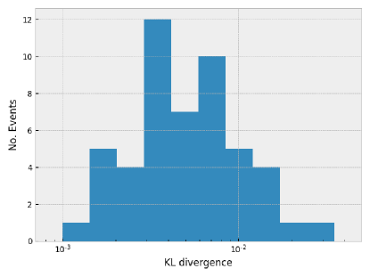
Figure 1: Histogram of KL divergences between our three-dimensional KDE $\hat{L}(x)$ and the inferred Gaussian approximation. GWTC-1 events are modeled using SEOBNRv3 (except GW180817, which uses IMRPhenomPv2NRT_lowSpin). GWTC-2 events are modeled using the preferred catalog samples.

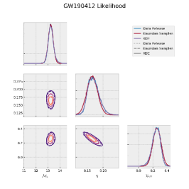
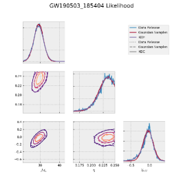
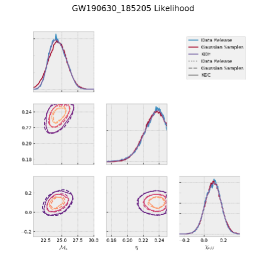
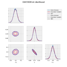
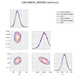
Figure 2: Illustrations of Gaussian fits for interesting events (e.g., where the peak likelihood is offset from equal mass). The one-dimensional figures along the diagonal of each corner plot show the inferred marginal likelihood Gaussian approximation (red), KDE approximation (purple), and reweighted original posterior samples (blue), where the reweighting converts to a uniform prior in ${\cal M}_{c},\eta,\chi_{\rm eff}$. The two dimensional marginalizations show the 25%, 50%, and 75% contour for the reweighted catalog (dotted), the KDE (solid), and the Gaussian (dashed). These events are all well-fit, including the high-mass event GW190521; see Figure 1 for quantitative measures of similarity.

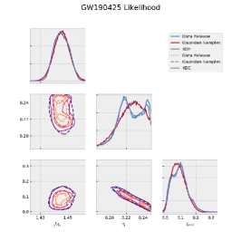
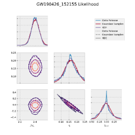
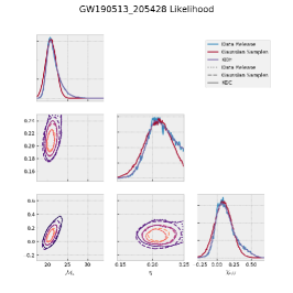
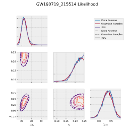
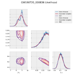
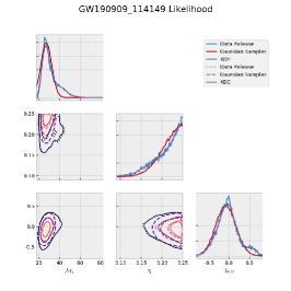
Figure 3: Selected Gaussian fits which omit some features of the estimated likelihood. The two cases of multimodal likelihoods are not well-fit by a single Gaussian, as are cases with a sharp spike or extra lump. GW190719 is interesting, in that one might expect this binary to have equal mass by visual inspection, but the peak observed in the fit is offset from $\eta=1/4$. Still, the Gaussian models presented boast a convincing goodness of fit estimate (Figure 1), and the offsets are small compared to statistical and astrophysical uncertainty.

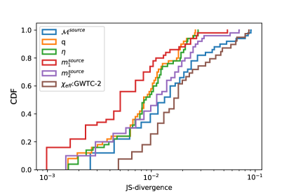
Figure 4: Cumulative distribution of JS divergences between input posterior distribution and one regenerated from the (three-dimensional) Gaussian likelihoods provided in this work.

We have evaluated our multivariate Gaussian approximations for all events, using GWTC-1 and GWTC-2 [5, 6]. For GWTC-1, SEOBNRv3 was used for each event apart from GW170817, for which IMRPhenomPv2NRT_lowSpin was used. For GWTC-2, the preferred samples from the catalog were used for each event. The parameters of these Gaussians are available at https://gitlab.com/xevra/nal-data. Figure 1 provides quantitative diagnostics of our goodness-of-fit for all events reported to date, for the three-dimensional space of fitting parameters. For almost all events, our multivariate Gaussian approximations provide an excellent approximation to the three-dimensional marginal distribution in ${\cal M}_{c},\eta,\chi_{\rm eff}$. As an illustration, Figure 2 compares our Gaussian approximations to the inferred three-dimensional marginal likelihood $\hat{L}$ for six selected events, including representative massive and low-mass compact binaries. For most events, the peak of our Gaussian approximation is consistent with equal mass; however, for many events, the Gaussian approximation is notably offset from the equal-mass line: GW170104, GW170809, GW190412, GW190426c, GW190503bf, GW190512at, GW190513bm, GW190519bj, GW190521r, GW190630ag, GW190706ai, GW190814, GW190828j, GW190929d. Given the fifty observations we focus on in this study, we would expect to find on average 2.5 events at least two standard deviations away from equal mass, even under the assumption that most events have mass ratios indistinguishable from unity. We find nine (three) events with mass ratios offset by at least one (two) standard deviation(s), which is consistent with that assumption.

Because our approximation works so well, we highlight in Figure 3 the few cases where our Gaussian approximation does not capture key features of the reported fiducial posterior. Only a handful of events at the lowest masses and/or associated with low SNR have features which are manifestly non-Gaussian in these three variables. As seen in Figure 3, only two events show notable multimodality in the inferred likelihood: the low-amplitude low-mass event (GW190425) and the oddly-behaved fiducial PE for GW190720. Even in these cases which proved difficult to fit, the Gaussian model produced has a low KL divergence relative to directly inferred Gaussian parameterizations, and we provide examples of few key events (Figure 1).

To further demonstrate the utility of these extremely simple approximations, we regenerate full six-dimensional posterior distributions, assuming the marginal likelihood only depends on ${\cal M}_{c},\eta,\chi_{\rm eff}$ according to our Gaussian approximation. We otherwise adopt comparable priors for mass and spin: uniform in (source-frame) component masses, uniform in component spin magnitudes, and isotropic in component spin directions. Figure 4 shows quantitative comparisons between our input posterior distribution and the posterior inferred from our Gaussian approximation. Precisely insofar as previous gravitational wave observations don’t constrain transverse spin, this three-dimensional likelihood approximation allows us to regenerate a full eight-dimensional posterior distribution which agrees extremely well with the full posterior distribution used to generate it. At very low mass, however, gravitational wave observations can and do modestly constrain transverse spins, so our three-dimensional approximation increasingly breaks down. In subsequent work, we will report on the agreement between ${\cal L}$ with more intrinsic and few extrinsic degrees of freedom (e.g., with all eight spin degrees of freedom, distance, and tides). However, for most applications of observations through GWTC-2, the simple three-dimensional approximation suffices.

IV Applications

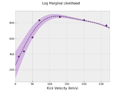
Figure 5: The likelihood that StarTrack simulations (points) represent physical assumptions, as a function of supernova natal recoil kick velocity. The dotted line is a Gaussian Process Regression (GPR) interpolation of this likelihood, and the region of one sigma is shaded.

One application of our fast normal approximate likelihoods is to quantitatively compare detailed compact binary formation models to gravitational wave observations. Simple parameterized phenomenological models can be efficiently compared to GW observations using previously-reported samples [34, 6]. By contrast, due to their computational complexity, physics-based models are customarily explored via Monte Carlo, propagating the results of many randomly selected initial conditions through their (at times stochastic) evolutionary model. Because both these simulations’ outputs and GW observations are represented by Monte Carlo samples, a continuous approximation of (at least) one set of samples is required to produce the net likelihood of the model, given GW observations. In this work, we will approximate the GW likelihood by normal distributions, and use the StarTrack binary evolution suite [35, 36, 37, 38]; see Appendix A for pertinent inputs.

Following our longer companion study [39], we evaluate the (marginal) inhomogeneous Poisson likelihood for existing GW observations, given each specific population synthesis model. We use the entire simulated merger population ($\sim 10^{8}$ samples); only a fast approximation like a multivariate normal makes calculations at this scale possible.

In this work, we report on a previously-reported and extensively-studied one-parameter family of binary evolution models, which varies only the strength of supernova natal recoil kicks on newly formed compact remnants. All input models are publicly available via www.syntheticuniverse.org [38].

Figure 5 shows our results for the M13–M19 (sub-model B) family of models. The solid lines show each model’s net likelihood. The dotted line and shaded region show the results of carefully interpolating between these models’ results with a Gaussian process, accounting for systematics in each evaluated likelihood. Consistent with several previous studies, we find the net likelihood peaks with kick velocities around $100{\rm km/s}$. Nominally, this peak reflects two factors which arise from the model’s predictions as weighted by GW search selection effects: the expected number of detections should be consistent with the observed count; and the distribution of observed masses should be consistent with the models’ selection-weighted predictions. However, in our simple application, the mass distribution of the M13–M19 models varies relatively little, so the strong peak in the overall likelihood principally reflects the point where the observed count is close to the expected count.

V Conclusions

Motivated by well-studied analytic approximations, we have introduced a straightforward but powerful technique to approximate existing posterior distributions via a Gaussian likelihood. We demonstrated this approach performs surprisingly well with just 3 key dimensions (${\cal M}_{c},\eta,\chi_{\textrm{eff}}$) for all events reported in GWTC-1 and GWTC-2.

In subsequent work, we comment on how well this approximation continues to perform when all intrinsic degrees of freedom, distance, and tides are included in previously reported-events.

The increasing degree of precision with which can be characterized may allow for better constrained parameterization for additional degrees of freedom in dimensions such as transverse spin for future events. We also expect to comment on how well this approach performs for such degrees of freedom as well in future work.

This extremely compact and analytically-tractable representation of GW observations will enable end-users to perform robust analyses with many inputs.

With modest extension to estimate the eigenvalues and eigenvectors of these Gaussians, via ansatz or interpolation, this work also provides a straightforward path toward generating extremely realistic synthetic GW catalogs. Such catalogs have wide application to investigate GW population astrophysics.

Appendix A Estimating StarTrack Model Likelihoods

In this section we briefly summarize the StarTrack simulation suite and the methods which allow us to draw conclusions from StarTrack populations [35, 36, 37, 38]. StarTrack evolves binary star systems, and considers a host of physical processes including accretion, tidal interactions, stellar wind, metallicity, gravitational radiation, magnetic braking, and supernova natal recoil kicks [35]. Populations are drawn at a distribution of redshifts, and are weighted appropriately to create accurate merger rate densities for those systems which become compact binaries that merge in cosmological time [40, 41, 42]. Cosmological postprocessing for StarTrack populations in a realistic spread of metallicities allows for the generation of a synthetic universe with a physically motivated population of compact binary merger rate densities [42]. These densities allow us to construct an estimate of the merger rate density $\rho_{i}(\mathbf{\lambda})$ for a given population (e.g., $i$ indexes M13, M14, etc), a physically scaled density function in merger parameters, $\mathbf{\lambda}$ [34].

In order to properly constrain formation parameters $\Lambda_{i}$, for a population $i$, we must calculate the joint likelihood for each population:

$$P(\{d_{j}\}|\Lambda_{i})=P(\mu_{i}|\Lambda_{i})\prod\limits_{j}P(d_{j}|\Lambda_{i})$$ (7)

Here, $\{d_{j}\}$ denotes a set of gravitational wave observations, individually $d_{j}$. The joint likelihood is derived from the marginalized event likelihood for each observation, $P(d_{j}|\Lambda_{i})$ and the inhomogeneous Poisson likelihood for the total number of observations of each type (the rate likelihood), $P(\mu_{i}|\Lambda_{i})$ [34]. In this study, the joint likelihood is dominated by the event likelihood, which changes more rapidly than the rate likelihood from one population to another. For a more diverse set of population models, both the rate likelihood and event likelihood will be important for constraining formation parameters.

A.0.1 Rate Likelihood

The probability that LIGO detection rates would match the expected rate within a population for each type of event $\alpha\in$ {BBH, BNS, NSBH} is given by the inhomogeneous Poisson likelihood [34]:

$$P(\mu_{\alpha,i}|\Lambda_{i})=\ e^{-{\mu_{\alpha,i}}}\frac{\mu_{i,\alpha}^{N_{\alpha}}}{N_{\alpha}!}$$ (8)

Here, $\mu_{\alpha,i}$ is the predicted detection rate for a population, and $N_{\alpha}$ is the number of published detections of each type for a given observing run. Therefore, the combined rate likelihood is

$$P(\mu_{i}|\Lambda_{i})=\prod\limits_{\alpha}\bigg{[}\frac{(\mu_{\alpha,i})^{N_{\alpha}}}{N_{\alpha}!}\bigg{]}e^{-\sum\limits_{\alpha}\mu_{\alpha,i}}=K_{i}e^{-\mu_{i}}$$ (9)

In our own work [39], we predict the expected detection rates for each population by the method outlined by Dominik et al. [42]

$$\mu_{det}=T_{\mathrm{obs}}\sum\frac{\mathrm{SFR}}{\Delta M_{f}}p_{\mathrm{det}}\frac{1}{1+z}\frac{dV_{c}}{dz}\frac{dz}{dt}\Delta t$$ (10)

$\mathrm{SFR}/\Delta M_{f}$ is a weighted star formation rate, and in our work is equivalent to $\rho_{i}(\mathbf{\lambda})$. $dV_{c}/dz$ is the differential comoving volume according to a conventional Planck2015 cosmology [43]. Additionally, $dz/dt=(1+z)H$, and $\Delta t=100\mathrm{Myr}$ is the cosmological time step. The detector sensitivity, $p_{\mathrm{det}}(w)$, is interpolated from results tabulated by other groups (https://pages.jh.edu/~eberti2/research/) [42]. The signal-to-noise ratio is interpolated using a sparse Gaussian process regression method, and evaluated for each merger sample [39]. All cosmological calculations are implemented with astropy [44].

A.0.2 Event Likelihood and Marginalization

The marginalized event likelihood $P(d_{j}|\Lambda_{i})$ must be calculated using the associated event likelihood $\mathcal{L}_{j}(\mathbf{\lambda})$ and normalized merger rate density function for each population, $\bar{\rho}(\mathbf{\lambda})$. For each of the $\leavevmode\nobreak\ 10^{8}$ sample binary mergers (samples are indexed by $k$) in a population with formation parameters $\Lambda_{i}$, each event likelihood must be calculated $\mathcal{L}_{j}(\lambda_{i,k})=P(d_{j}|\lambda_{i,k}\Lambda_{i})$. With the same indexing, the normalized merger rate densities for each sample are $\omega_{i,k}$. That evaluation would not be possible without an approximate model for the event likelihood which could be evaluated in a small fraction of a second. We use Normal approximations to the likelihood, such as those which appear in this publication.

The marginalization is as follows

$$P(d_{j}|\Lambda_{i})=\int\limits_{\{\mathbf{\lambda}\}}P(d_{j}|\mathbf{\lambda},\Lambda_{i})P(\mathbf{\lambda}|\Lambda_{i})\mathrm{d}\mathbf{\lambda}=\int\limits_{\{\mathbf{\lambda}\}}\bar{\rho}_{i}(\mathbf{\lambda})\mathcal{L}_{j}(\mathbf{\lambda})\mathrm{d}\mathbf{\lambda}$$ (11)

This brings us to our discrete expression [34] for the joint likelihood:

$$P(\{d_{j}\}|\Lambda_{i})\propto K_{\mathrm{rate},i}\mathrm{e}^{-\mu_{\mathrm{det},i}}\prod\limits_{j}\bigg{[}\sum\limits_{k}\mathcal{L}_{j}(\lambda_{i,k})\omega_{i,k}\bigg{]}$$ (12)