The Poissonian Origin of Power Laws in Solar Flare Waiting Time Distributions

Abstract

In this study we aim for a deeper understanding of the power law slope, $\alpha$, of waiting time distributions. Statistically independent events with linear behavior can be characterized by binomial, Gaussian, exponential, or Poissonian size distribution functions. In contrast, physical processes with nonlinear behavior exhibit spatio-temporal coherence (or memory) and “fat tails” in their size distributions that fit power law-like functions, as a consequence of the time variability of the mean event rate, as demonstrated by means of Bayesian block decomposition in the work of Wheatland et al. (1998).

In this study we conduct numerical simulations of waiting time distributions $N(\tau)$ in a large parameter space for various (polynomial, sinusoidal, Gaussian) event rate functions $\lambda(t)$, parameterized with an exponent $p$ that expresses the degree of the polynomial function $\lambda(t)\propto t^{p}$. We derive an analytical exact solution of the waiting time distribution function in terms of the incomplete gamma function, which is similar to a Pareto type-II function and has a power law slope of $\alpha=2+1/p$, in the asymptotic limit of large waiting times. Numerically simulated random distributions reproduce this theoretical prediction accurately. Numerical simulations in the nonlinear regime ($p\geq 2$) predict power law slopes in the range of $2.0\leq\alpha\leq 2.5$. The self-organized criticality model yields a prediction of $\alpha=2$. Observations of solar flares and coronal mass ejections (over at least a half solar cycle) are found in the range of $\alpha_{obs}\approx 2.1-2.4$. Deviations from strict power law functions are expected due to the variability of the flare event rate $\lambda(t)$, and deviations from theoretically predicted slope values $\alpha$ occur due to the Poissonian weighting bias of power law fits.

1 Introduction

Waiting time analysis, a branch of statistical methods to discriminate between random processes (with linear behavior) and processes with intermittence, clustering, and memory (with nonlinear behavior) has become a wide-spread industry to study astrophysical data. The hallmark of uncorrelated random processes is their characterization by binomial, Gaussian, Poissonian, or exponential distribution functions, while nonlinear avalanche-like processes reveal power law-like distribution functions. Applications of such diagnostic tests have been explored in solar flares (Wheatland et al. 1998; Boffetta et al. 1999; Wheatland 2000a; Leddon 2001; Lepreti et al. 2001; Norman et al. 2001; Wheatland and Litvinenko 2002; Grigolini et al. 2002; Aschwanden and McTiernan 2010; Gorobets and Messerotti 2012; Hudson 2020; Morales and Santos 2020), in coronal mass ejections (Wheatland 2003; Yeh et al. 2005; Wang et al. 2013, 2017); in solar energetic particle events (Li et al. 2014); in solar wind discontinuities and its intermittent turbulence (Carbone et al. 2002; Greco et al. 2009; Wanliss and Weygand 2007), in heliospheric type III radio burst storms (Eastwood et al. 2010), in solar wind switchback events (Bourouaine et al. 2020; Dudok de Wit et al. 2020; Aschwanden and Dudok de Wit 2021), in the cyclic behavior of the solar dynamo over millennia (Usoskin et al. 2017), in active and inactive M-dwarf stars (Hawley et al. 2014; Li et al. 2018), in the avalanche dynamics of radio pulsar glitches (Melatos et al. 2008; 2018), in magnetar bursts (Cheng et al. 2020), stellar gamma-ray bursts (Guidorzi et al. 2015; Yi et al. 2016), black hole systems (Wang et al. 2015, 2017), and in plasma physics experiments (Sanchez et al. 2002). For a review of waiting time distributions in astrophysics see textbook Chapter 5 in Aschwanden (2011).

The power law behavior of waiting time (or laminar time intervals) has been interpreted in terms of magnetohydrodynamic (MHD) turbulence (Boffetta et al. 1999; Carbone et al. 2002; Bourouaine et al. 2020), complementary to self-organized criticality models, since both types of models can produce bursty avalanches, intermittency, power law-like size distributions, and 1/f-spectra (Carbone et al. 1999). Alternative approaches of analyzing flare waiting times includes Bayesian decomposition (Wheatland and Litvinenko 2002; Wheatland 2004; Wheatland and Craig 2006), information theory and Shannon entropy (Snelling et al. 2020). Interestingly, the waiting time distribution of pulses from active black hole systems exhibit the same power law slopes as measured in solar flares, $\alpha\approx 2.0$, which indicates some universality (Wang et al. 2015; Yi et al. 2016).

Besides the diagnostic capability of waiting time distributions, which is exploited in many of these studies, there is almost no study that attempts to explain the numerical value of the power law slope $\alpha$ in a waiting time distribution function, which represents a statistical invariant. We cannot claim that we understand waiting time distributions as long as we do not have a physical model that predicts the observed power law slopes. Furthermore, it has not yet been demonstrated whether power laws exist at all (Stumpf and Porter 2012) in waiting time distributions, or what detailed mathematical function is to be expected. Recent studies identify Pareto type-II functions to fit waiting time distributions (Aschwanden and McTiernan 2010; Aschwanden and Freeland 2012; Aschwanden and Dudok de Wit 2021), which exhibit a power law-like part in the asymptotic limit only.

In this Paper we calculate analytical exact and approximative solutions of waiting time distributions (Section 2 and Appendices A, B, and C). We present new analytical solutions in terms of the gamma function, the incomplete gamma function, the Pareto type-II function, while another exact analytical solution was recently found in terms of Bessel functions (Nurhan et al. 2021). We test the analytical solutions with numerical simulations of random waiting times (Section 3). We explore the variability of the event rate function $\lambda(t)$, which appears to be a key parameter in the calculation of the power law slope $\alpha$ of waiting times, by performing a parametric study of the power law slope $\alpha$ and nonlinearity parameter $p$ of the event rate evolution (Section 3). In the discussion section we juxtapose observed, theoretical, and numerical waiting time distributions, examine the existence of power laws and their expected deviations, as well as their role in self-organized criticality models (Section 4). We complete the paper with a summary of conclusions (Section 5).

2 Theory

2.1 Stationary Waiting Time Distributions

Statistical probability distributions $N(\tau)d\tau$ of event waiting times, $\tau$, have distinctly different mathematicl functions, depending on whether their generation is produced by a linear or by a nonlinear process. If statistical events are produced by a linear process, the resulting size distribution $N(x)\ dx$ or waiting time distribution $N(\tau)\ d\tau$ follows Poissonian statistics, which can be fitted by an exponential function,

$$N(\tau)\ d\tau=\lambda_{0}\ \exp{\left[-\lambda_{0}\tau\right]}\ d\tau\ ,$$ (1)

where $N(\tau)d\tau$ is the number of events per bin $d\tau$, $\lambda_{0}=1/\tau_{0}$ is the mean event rate or mean reciprocal waiting time, i.e., $\tau_{0}=T/N_{0}$, with $T$ being the total duration of an observed data set, and $N_{0}$ is the total number of events detected during this time interval. The total number of events is $N_{0}$,

$$\int_{0}^{\infty}N(\tau)d\tau=N_{0}\ .$$ (2)

In contrast, if a statistical sample is produced by a nonlinear process, the “fat-tail” of their distribution function becomes important and the resulting size distribution or waiting time distribution $N(\tau)$ fits a power law distribution function,

$$N(\tau)\ d\tau\propto\ \tau^{-\alpha}\ d\tau\ ,$$ (3)

with power law slope $\alpha$. This formalism is valid for a large variety of nonlinear events, including solar and stellar flares, terrestrial catastrophes, also known as avalanche events in the parlance of self-organized criticality systems.

How do we distinguish between stationary and non-stationary statistics? Stationary Poisson processes have a constant event rate function $\lambda_{0}$ within the statistical uncertainties in any time interval of a considered data set. Non-stationary data samples have a variable mean event rate $\lambda(t)$ as a function of time $t$ (also called flare rate function). In the case of solar flares, for instance, the flare event rate varies by factors of $\approx 10^{2}-10^{3}$ between the solar cycle ($T\approx 11$ years) minimum and maximum. In the following we will use the terms event rate function and flare rate function $\lambda(t)$ interchangeably.

2.2 Non-Stationary Waiting Time Distributions

We define non-stationary waiting time distribution functions with a time-dependent flare rate function $\lambda(t)$, which is a generalization from the constant $\lambda_{0}$ (Eq. 1) to a time-dependent mean flare rate $\lambda(t)$,

$$N(\tau)\ d\tau=\lambda(t)\ \exp{[-\lambda(t)\ \tau]}\ d\tau\ .$$ (4)

Subdividing a waiting time distribution into a piece-wise constant Poisson process with rates $\lambda_{i}$ and time intervals $\tau_{i}$, it can be approximated by (Wheatland 2000b; 2001),

$$N(\tau_{i})\approx\sum_{i}\varphi_{i}\lambda_{i}\exp{[-\lambda_{i}\tau_{i}]}\ ,$$ (5)

where

$$\varphi_{i}={\lambda_{i}\tau_{i}\over\sum_{i}\lambda_{i}\tau_{i}}\ ,$$ (6)

is the fraction of events associated with a given rate $\lambda_{i}$. Inserting the fractions $\varphi_{i}$ (Eq. 6) into the waiting time probability distribution function (Eq. 5) we obtain,

$$N(\tau_{i})\approx{\sum_{i}\lambda_{i}^{2}\ \tau_{i}\ \exp{[-\lambda_{i}\tau_{i}]}\over\sum_{i}\ \lambda_{i}\ \tau_{i}}\ ,$$ (7)

which in the asymptotic limit of arbitrary small Bayesian time intervals approaches the integral $N(\tau)$,

$$N(\tau)={\int_{0}^{T}\lambda(t)^{2}\ \tau\ \exp{[-\lambda(t)\tau]\ dt}\over\int_{0}^{T}\ \lambda(t)\ \tau\ dt}={\int_{0}^{T}\lambda(t)^{2}\ \exp{[-\lambda(t)\tau]\ dt}\over\int_{0}^{T}\ \lambda(t)\ dt}\ .$$ (8)

The right-hand side equation simplifies somewhat with the cancellation of the variable $\tau$ in both the numerator and denominator.

Note that our treatment of non-stationary Poisson processes follows the previous work of Wheatland (2000b; 2001), which is related to the concepts of “mixed Poisson”, “compound Poisson”, “contagion Poisson”, “Poisson autoregression”, and “Poisson point” processes (Kingman 1993; Grandell 1997; Streit 2010).

2.3 Flare Rate Functions

In non-stationary waiting time distributions, the temporal variability of the mean event rate $\lambda(t)$ needs to be defined, in order to calculate the waiting time distribution $N(\tau)$ (Eq. 8). In order to minimize the number of free parameters, following the principle of Occam’s razor, we define here non-stationary event rate functions $\lambda(t)$ that have three parameters only $(T,\lambda_{0},p)$. These flare rate functions have: (i) a total duration $T$ and a mean event rate $\lambda_{0}$, (ii) are symmetric in the time interval before and after the peak time $t=T/2$, and (iii) vary the shape of the (flare) event rate function (as a function of time) by a single exponent $p$ (also called degree or order of polynomial), to which we refer as nonlinearity parameter also. We define three different flare rate function models, including the polynomial, sinusoidal, and Gaussian function,

$$\lambda(t)=\lambda_{0}\left\{\begin{array}[]{ll}\left({T/2-|t-T/2|\over T/2}\right)^{p}&{\rm Polynomial\ model}\\ \left(\sin{\left[\pi{t\over T}\right]}\right)^{p}&{\rm Sinusoidal\ model}\\ \left(\exp{\left[-{(T/2-t)^{2}\over 2\sigma^{2}}\right]}\right)^{p}&{\rm Gaussian\ model}\end{array}\right.\ .$$ (9)

These time-dependent functions $\lambda(t)$ are suitable to represent the time variation of a cycle, such as the solar cycle of $T\approx 11$ years. For the parameter $p=1$, the polynomial model mimics a simple triangular function with linear rise time and decay time, for $p=2$ a quadratic function, for $p=1/2$ a square root function, and for large exponents $p\gg 1$ it asymptotically approaches the Dirac delta function. The parameter space of $t$ and $\lambda(t)$ is shown in Fig. 1 for the polynomial flare rate function, which illustrates that functions $\lambda(t)$ with degree $p=0.1,...,10$ cover most of the $\lambda(t)$ parameter space.

Similar time profiles are formulated for the sinusoidal and Gaussian function (Eq. 9). The Gaussian width $\sigma$ is defined from the full width at half maximum (FWHM) being equal to the half duration, i.e., FWHM=T/2, and $\sigma=(T/4)/\sqrt{2\ln 2}$. The selection of three different functional forms (polynomial, sinusoidal, and Gaussian) allows us to explore systematic errors in the power law slope of waiting time distributions, which are generally larger than the formal errors obtained from least-square fitting. Another motivation for the choice of our selection of flare rate functions $\lambda(t)$ is the availability of analytical exact solutions, for the polynomial model (see Section 2.4 and Appendix A), for the sinusoidal flare rate model (Nurhan et al. 2021), for the Gaussian flare rate model (Appendix C), as well as for the Pareto type-II distribution function (Appendix B).

2.4 Exact Solution of Waiting Time Distribution

We derive here an analytical exact solution of the waiting time distribution $N(\tau)d\tau$ (Eq. 8),

$$N(\tau)={2\int_{0}^{T/2}\lambda(t)^{2}\ \exp{[-\lambda(t)\tau]\ dt}\over 2\int_{0}^{T/2}\ \lambda(t)\ dt}\ ,$$ (10)

for the general case of a flare rate function $\lambda(t)$, chosen symmetrically about the peak time $t=T/2$ in the time range $0\leq t\leq T$, in terms of a polynomial with degree $p$ (Eq. 9),

$$\lambda(t)=\lambda_{0}\left({t\over T/2}\right)^{p}\ .$$ (11)

Inserting Eq. (11) into Eq. (10) leads to,

$$N(\tau,p)={\int_{0}^{T/2}\lambda_{0}^{2}\ [t/(T/2)]^{2p}\ \exp{[-\lambda_{0}\ [t/(T/2)]^{p}\ \tau]\ dt}\over\int_{0}^{T/2}\ \lambda_{0}\ [t/(T/2)]^{p}\ dt}\ .$$ (12)

Substituting the variable $x=t/(T/2)$, with $dx/dt=1/(T/2)$ and $dt=dx(T/2)$, renders Eq. (12) as,

$$N(\tau,p)={\int_{0}^{1}\lambda_{0}^{2}\ x^{2p}\ \exp{[-\lambda_{0}\ x^{p}\tau]\ dx}\over\int_{0}^{1}\ \lambda_{0}\ x^{p}\ dx}\ ,$$ (13)

where the integral limits change from $t=[0,T/2]$ to $x=[0,1]$. The integral in the denominator of Eq. (13) is simply,

$$\int_{0}^{1}\lambda_{0}\ x^{p}\ dx={\lambda_{0}\over(p+1)}\ ,$$ (14)

while the integral $I(\tau,p)$ in the numerator of Eq. (10) is,

$$I(\tau,p)={\int_{0}^{1}\lambda_{0}^{2}\ x^{2p}\ \exp{[-\lambda_{0}\ x^{p}\tau]\ dx}}\ .$$ (15)

We change the variable $y=x^{p}$, or $x=y^{1/p}$, with the differential $dx=(1/p)y^{(1-p)/p}\ dy$, which yields,

$$I(\tau,p)=\int_{0}^{1}{\lambda_{0}^{2}\over p}y^{(1+p)/p}\ \exp{[-\lambda_{0}\ \tau\ y]}\ dy\ .$$ (16)

In the limit of $\tau\mapsto\infty$, the exponential factor drops very fast, so that the upper integral limit is of order $O(e^{-\beta})$, where $\beta$ is defined by

$$\beta=\lambda_{0}\tau\ ,$$ (17)

yielding,

$$I(\tau,p)=\int_{0}^{1}{\lambda_{0}^{2}\over p}y^{(1+p)/p}\ \exp{[-\beta\ y]}\ dy\ .$$ (18)

Substituting $\beta$ with $q=\beta\ y$ and $dq=\beta\ dy$,

$$I(\tau,p)\approx{\lambda_{0}^{2}\over p\ \beta^{2+1/p}}\int_{0}^{\infty}\ q^{(1+p)/p}\ \exp{[-q]}\ dy\ ,$$ (19)

leads to the gamma function $\Gamma$ (Bronstein and Semendjajew 1960),

$$\Gamma\left(\alpha\right)=\int_{0}^{\infty}q^{(\alpha-1)}\ \exp{[-q]}\ dq\ ,$$ (20)

and the integral over the range $q=[0,\infty]$ is, in the asymptotic expansion of the exact solution,

$$I(\tau,\alpha)\approx{\lambda_{0}^{2}\over p\ \beta^{\alpha}}\ \Gamma\left({\alpha}\right)\ ,$$ (21)

with the power law slope $\alpha$,

$$\alpha=2+{1\over p}\ .$$ (22)

Combining this expression with the denominator integral $\lambda_{0}/(p+1)$ (Eq. 14), we obtain an approximation of the waiting time distribution function,

$$N(\tau,\alpha)\approx\lambda_{0}\left({\alpha-1}\right)\ \Gamma{\left(\alpha\right)}\ {(\lambda_{0}\ \tau)}^{-\alpha}\ .$$ (23)

The exact solution of this integral is the incomplete gamma function (Bronstein and Semendjajew 1960),

$$\gamma\left(\alpha,\beta\right)=\int_{0}^{\beta}q^{(\alpha-1)}\ \exp{[-q]}\ dq\ ,$$ (24)

where the integral boundaries are $q=[0,\beta]$, in contrast to $q=[0,\infty]$ in the gamma function. The exact solution of the waiting time distribution as a function of the waiting time $\tau$ and nonlinearity parameter $p$ of the flare rate function $\lambda(t)\propto t$ reads then in the final form as,

$$N(\tau,\alpha)=\lambda_{0}\left({\alpha-1}\right)\gamma\left(\alpha,\lambda_{0}\tau\right)\ (\lambda_{0}\tau)^{-\alpha}\ .$$ (25)

The power law slope $\alpha=(2+1/p)$ can approximately be expressed in terms of the gamma function $\Gamma$, but the exact solution has an additional dependence of the waiting time $\tau$ in the incomplete gamma function $\gamma$ (Eq. 25).

Alternative solutions of the waiting time distribution $N(\tau)$ can be obtained also for Pareto Type-II distribution functions, which is presented in Appendix B. All solutions, the Gamma function $\Gamma$ solution (Eq. 21), the incomplete Gamma function $\gamma$ solution (Eq. 25), and the Pareto type-II distribution exhibit the same characteristics: The steepest power law slope is in the asymptotic limit of the largest waiting times, and a gradual rollover and flattening to a constant value occurs at the shortest waiting times, as illustrated in Fig. 2.

2.5 Self-Organized Criticality Model

There are very few studies that provide a prediction or physical model for the power law slope $\alpha$ of waiting time distributions. One of them is the fractal-diffusive avalanche model of a slowly-driven self-organized criticality (FD-SOC) system (Aschwanden 2012, 2014; Aschwanden and Freeland 2012; Aschwanden et al. 2016), which has has been further developed from the original version of SOC concepts (Bak et al. 1987; 1988). It is based on a scale-free (power law) size distribution function $N(L)$ of avalanche (or flare) length scales $L$,

$$N(L)\ dL\propto L^{-d}\ dL\ ,$$ (26)

with $d$ the Euclidean spatial dimension (which can have values of d=1, 2, or 3), defining a reciprocal relationship between the spatial size $L$ and the occurrence frequency $N(L)$.

In the FD-SOC model, the transport process of an avalanche is described by classical diffusion, which obeys the scaling law,

$$L\propto T^{\beta/2}\ ,$$ (27)

with $\beta=1$ for classical diffusion. Substituting the length scale $L\propto T^{\beta/2}$ with the duration $T$ of an avalanche event, using Eq. (26-27) and the derivative $dL/dT=T^{\beta/2-1}$, predicts a power law distribution function for the size distribution of time durations $T$,

$$N(T)\ dT=N(T[L])\left({dL\over dT}\right)\ dT\ \propto\ T^{-[1+(d-1)\beta/2]}dT\ \propto\ T^{-\alpha_{\tau}}\ dT\ \approx\ T^{-2}dT\ .$$ (28)

For standard parameters $d=3$ and $\beta=1$, it defines the waiting time power law slope $\alpha_{\tau}$,

$$\alpha_{\tau}=1+(d-1)\beta/2=2\ .$$ (29)

We can now estimate the size distribution of waiting times by assuming that the avalanche durations represent upper limits to the waiting times $\tau$ during flaring time intervals, while the waiting times become much larger during quiescent time periods. Such a bimodal size distribution with a power law slope of $\alpha_{\tau}\lower 1.72218pt\hbox{$\;\buildrel<\over{\scriptstyle\sim}\;$}2$ at short waiting times ($\tau\leq\tau_{e}$), and an exponential-like cutoff function at long waiting times $(\tau\geq\tau_{e})$ is approximately,

$$N(\tau)\ d\tau=\left\{\begin{array}[]{ll}\tau^{-2}&{\rm for}\ \tau\ll\tau_{e}\\ \tau^{-2}\exp(-\tau/\tau_{e})&{\rm for}\ \tau\lower 1.72218pt\hbox{$\;\buildrel>\over{\scriptstyle\sim}\;$}\tau_{e}\\ \end{array}\right.\ .$$ (30)

Thus, this FD-SOC model predicts a power law with a slope of $\alpha\approx 2.0$ in the inertial range, and a steepening cutoff function at longer waiting times.

3 Numerical Simulations and Analysis

3.1 Power Law Fitting Method

In this study we employ numerical simulations of waiting time distributions, using a random generator, a sorting algorithm, and a standard least-square minimization algorithm from the Interactive Data Language (IDL) software. For a stationary waiting time distribution we generate a random sample of $N_{0}$ values $t_{i}$, $i=1,...,N_{0}$, that are equally distributed in a unity time interval $[0,1]$. Then we run a sorting algorithm that sorts the values $t_{i}$ in a monotonically increasing rank order,

$$0<t_{1}<t_{2}<...<t_{N}$$ (31)

from which a series of $(N_{0}-1)$ positive time intervals $\tau$ can be obtained,

$$\tau_{i}=(t_{i+1}-t_{i})\ ,\quad i=1,2,...,N_{0}-1\ .$$ (32)

We sample the waiting times $\tau_{i}$ in a log-log histogram (Eq. 3) and fit the power law slope $\alpha$ in a suitable inertial (scale-free) range, using a standard least-square optimization algorithm,

$$\chi=\sqrt{{1\over(n_{bin}-n_{par})}\sum_{j=1}^{n_{bin}}{[N^{theo}(x_{j})-N^{obs}(x_{j})]^{2}\over\sigma_{j}^{2}}}\ ,$$ (33)

where $x_{j},j=1,...,n_{j}$ are the counts per bin width, $N^{theo}(x_{j})$ is the number counts of the theoretical model, $N^{obs}(x_{j})$ is the observed number counts, $n_{bin}$ is the number of the histogram bins, and $n_{par}$ is the number of free parameters of the fitted model functions. The estimated uncertainty of counts per bin, $\sigma_{j}$, is according to Poisson statistics,

$$\sigma_{j}={\sqrt{N_{j}\Delta x_{j}}\over\Delta x_{j}}\ ,$$ (34)

where $\Delta x_{j}$ is the (logarithmic) bin width. The goodness-of-fit $\chi$ quantifies which theoretical model distribution is consistent with the (observed) data. The uncertainty $\sigma_{\alpha}$ of the best-fit power law slope $\alpha$ is estimated from

$$\sigma_{\alpha}={\alpha\over\sqrt{N_{0}}}\ ,$$ (35)

with $N_{0}$ the total number of events in the entire size distribution (or in the fitted range).

The log-log histogram of the waiting times $\tau$ is sampled with a resolution of $n_{bin}=6$ bins per decade, typically for a sample of $N_{0}\approx 10^{4}$ events. The power law fit is performed with a least-square fit in the range of $[x_{0},x_{2}]$, where the lower bound $x_{0}$ is defined by the maximum of the log-log waiting time histogram, and a margin of $d_{bin}=1$ bin above $x_{0}$ is ignored in the power law fit in order to minimize the influence of the roll-over in the least-square fit of the power law slope. The upper bound $x_{2}$ of the inertial range is given by the largest waiting time. The data analysis performed here employs identical methods as in other studies (Aschwanden and McTiernan 2010; Aschwanden 2015, 2019a, 2019b; Aschwanden and Dudok de Wit 2021).

It is widely known that fitting on a log-log scale is biased and inaccurate, while using a maximum likelihood estimation is more robust (Goldstein et al. 2004; Newman 2005; Bauke 2007). We take this into account by using the Poissonian error estimate (Eq. 35). However, while this improves the formal error, there is a much larger systematic error due to deviations from ideal power laws (Stumpf and Porter 2012). One of the major goals of this paper is to pin down such systematic errors by calculating the exact analytical solutions of waiting time distributions, which are generally not ideal power laws, but rather convolutions with the (incomplete) Gamma function.

3.2 Analytical Solution Versus Numerical Simulation

In principle, there are three different methods of calculating a waiting time distribution: (i) by an analytical solution, (ii) by numerical integration of the analytical integral equation (Eq. 8), and (iii) by sampling of numerically simulated events, which essentially is a Monte Carlo simulation method. The problem is posed by the integral equation of the probability distribution function $N(\tau)$ as a function of the waiting time $\tau$ (Eq. 8) and a chosen flare rate function $\lambda(t)$ (for instance the flare rate functions given in Eq. 9).

We juxtapose the numerically simulated waiting time distributions (histogram in Fig. 2), the power law fit in the inertial range of this histogram (dashed line in Fig. 2), the exact analytical solution according to Eq. (A6) given in Appendix A (thick solid curve in Fig. 2), and the Pareto type-II approximation Eq. (B3) (thin solid curve in Fig. 2). We see that the power law slope of the exact analytical solution, $\alpha_{exact}=3.00$, is significantly steeper than the slope of the power law fit to the simulated data, $\alpha=2.67\pm 0.03$, by a factor of $\alpha_{exact}/\alpha_{fit}=1.12$ (or 12%). This occurs because of the Poissonian weighting bias, which produces the smallest uncertainties $(\sigma\propto\sqrt{N})$ in the bins at the lower bound of the inertial range (at $x_{0}$), and thus constrains the power law fit there most. We found that relatively small samples with $N_{0}\approx 10^{3}$ events provide a better overall fit (according to the goodness-of-fit criterion Eq. 33), rather than large samples of order $N_{0}\lower 1.72218pt\hbox{$\;\buildrel>\over{\scriptstyle\sim}\;$}10^{5}$, for the same reason (of the weighting by Poisson statistics). The formal error from $\chi$-square fitting is typically $\approx 1\%$ for a sample size of $N_{0}\approx 10^{4}$, according to Poisson statistics (i.e., $\sigma\propto\sqrt{N_{0}}$), which is generally smaller than the systematic errors (in the order of $\lower 1.72218pt\hbox{$\;\buildrel>\over{\scriptstyle\sim}\;$}10\%$).

3.3 Multi-Poissonian Waiting Time Distributions

We show the results of some numerical simulations in Figs. (3) and (4). In Fig. (3) we show six simulation runs with varying temporal resolution. In the first case (Fig. 3a) the time resolution is equal to the total duration of the observations, $\Delta t=T$, which corresponds to a constant flare rate $\lambda(t)=\lambda_{0}$, yielding a perfect exponential waiting time distribution (Fig. 3g), as defined in Eq. (1). When we increase the resolution to $\Delta t=T/2$ (Fig. 3b), we see that the waiting time distribution $N(\tau)$ exhibits a double hump (Fig. 3h), which is the superposition of two flare rates, one at the solar cycle minimum and one at the solar cycle maximum. This double hump structure persists on a weaker level when we increase the time resolution to $\Delta t=T/4$ and T/8 (Figs. 3i and 3j), but is morphing towards a perfect power law distribution for $\Delta t=T/16$ and T/32 (Figs. 3k and 2l). This series of simulations demonstrates most clearly the Poissonian origin of power laws. Essentially, broadening the flare rate $\lambda(t)$ transforms the waiting time distribution $N(\tau)$ from an exponential (Eq. 1) to a power law distribution function (Eq. 3). The theoretical slope of a continuous sinusoidal model with $\lambda(t)\propto\sin{(t)}^{2}$ with exponent $p=2$ is $\alpha=2+1/p=2.5$ (Eq. 22), which agrees well with the simulations with $\alpha\approx 2.5\pm 0.1$ (Fig. 3).

3.4 Variation of Flare Rate Functions

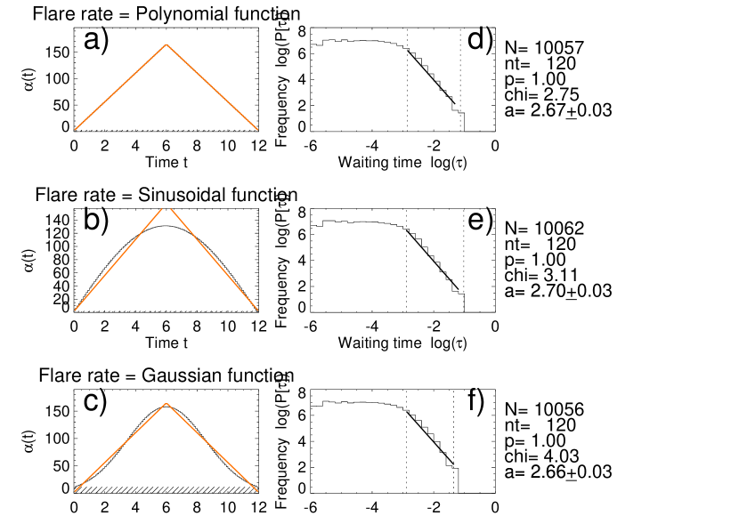
Figure 4: Three cases of numerical simulations of the time evolution of the polynomial (a,d; in red color), the sinusoidal (b,e), and the Gaussian (c,f) flare rate function $f(t)$ (left panels a-c) are shown, for linear flare rate changes ($p=1$). The corresponding waiting time distributions (right panels d-f) are computed for the exponent $p=1$, and yield a best-fit power law slope of $a\approx 2.7$. The power law slope values are not corrected for the Poissonian weighting bias.

In Fig. 4 we show three examples of simulated shapes of flare rate functions $\lambda(t)$, selecting one example (with parameter $p=1$) from each of the three (polynomial, sinusoidal, and Gaussian) model groups. The first case is generated by a linear rise time and decay time in the flare rate function $\lambda(t)\propto t$, which is simply a polynomial function with exponent $p=1$. The time evolution, analytically defined by Eq. (9), is shown in Fig. (4a), and the resulting waiting time distribution $N(\tau)$ is approximated by a power law slope with value $\alpha=2.67\pm 0.03$ (Fig. 4d), in an inertial range of $\tau\approx 10^{-3},...,10^{-1}$, from a sample of $N_{0}=1.0\times 10^{4}$ events. The same fit is shown in Fig. 2, juxtaposed to the analytical solution and the Pareto type-II approximation. The total duration of the simulation is $T=11$ years (to mimic the solar cycle), and the number of temporal Bayesian blocks in the flare rate function is chosen in $N_{t}=120$ time bins here, corresponding to a bin width of $dt=T/N_{t}\approx 0.1$ (years). Similarly, the flare rate time profiles $\lambda(t)$ is shown for a sinusoidal (Fig. 4b) and for a Gaussian model (Fig. 4c). The various models of flare rate functions $\lambda(t)$ shown in Fig. 4 illustrate that they all produce power law-like waiting time distributions $N(\tau)$ with slopes that are almost identical, in the range of $\alpha\approx 2.66-2.70$, for a nonlinearity parameter of $p=1$. Hence, the power law slopes $\alpha$ are not very sensitive to the detailed shape of the flare rate functions $\lambda(t)$, as long as a similar range of flare rates is covered. The Gaussian event rate function, however, has a finite value at $t=0$ and $t=T$, which affects the power law slope somewhat, compared with the polynomial and the sinusoidal case that have zero-values, $\lambda(t=0)=0$ and $\lambda(t=T)=0$.

3.5 Power Law Slopes of Waiting Time Distributions

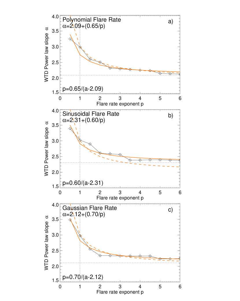
Figure 5: (a) Relationship between waiting time power law slope $\alpha$ and the flare rate function exponent $p$, computed by numerical simulations (diamonds) for three different (polynomial, sinusoidal, Gaussian) flare rate model functions, and fitted with the function $\alpha=\alpha_{0}+a_{1}/p$. The theoretical prediction $\alpha=2+1/p$ is indicated with dashed curves. The fitted power law slopes are corrected by a factor of $q_{corr}=1.12$ (Fig. 2) to compensate for the Poissonian weighting bias.

Since we are interested in quantifying the waiting time distribution $N(\tau)\propto\tau^{-\alpha}$ from first principles, we need a relationship between the power law slope $\alpha$, which is an observable, and the free parameter $p$ that characterizes the flare rate function $\lambda(t)\propto t^{p}$ (Eq. 9). We apply linear regression fits and show the values of the best-fit power law slopes $\alpha(p)$ as a function of the flare rate function exponent $p$ in Fig. (5), for a range of p=0.5 - 6.0 (tabulated in Table 1). Each value of the 36 runs corresponds to a separate numerical simulation. We find that the relationship between the two parameters $\alpha$ and $p$ can be determined by linear regression fits (Fig. 5),

$$\alpha(p)\approx\left\{\begin{array}[]{ll}2.09+0.65/p&\quad{\rm Polynomial\ model}\\ 2.31+0.60/p&\quad{\rm Sinusoidal\ model}\\ 2.12+0.70/p&\quad{\rm Gaussian\ model}\\ \end{array}\right.\ ,$$ (36)

Note that we applied the correction factor $\alpha_{corr}/\alpha_{fit}=1.12$ to the observed (or numerically simulated) power law slopes $\alpha_{fit}$ due to the Poissonian weighting bias (see Section 3.2 and Fig. 2). These best-fit relationships reproduce the chief features of the theoretical prediction ($\alpha=2+1/p$), based on the gamma function $\Gamma$ (Eq. 23) in the approximative case, or based on the incomplete gamma function $\gamma$ (Eq. 25) in the exact analytical solution: (i) An asymptotic value of $a\approx 2.0$ is obtained in the nonlinear regime ($p\mapsto\infty$), and (ii) an asymptotic value of $\alpha\lower 1.72218pt\hbox{$\;\buildrel>\over{\scriptstyle\sim}\;$}2$ is reached in the linear regime ($p\lower 1.72218pt\hbox{$\;\buildrel<\over{\scriptstyle\sim}\;$}1$). The polynomial flare rate relationship is shown in Fig. (5a), while similar values were obtained for the sinusoidal (Fig. 5b) and the Gaussian flare rate model (Fig. 5c). An exact solution for a sinusoidal flare rate function including a full period and its waiting time distribution is given in Nurhan et al. (2021) with $\alpha=2.5$.

In practice, the power law slope $\alpha_{pred}$ can now be predicted from the observed parameter $p_{obs}$ in the flare rate function $\lambda(t)\propto t^{p}$,

$$\alpha_{pred}=2+{1\over p_{obs}}\ ,$$ (37)

or vice versa, the nonlinearity parameter $p_{pred}$ can be predicted from from fitting the power law slope $\alpha_{obs}$,

$$p_{pred}={1\over\alpha_{obs}-2}\ .$$ (38)

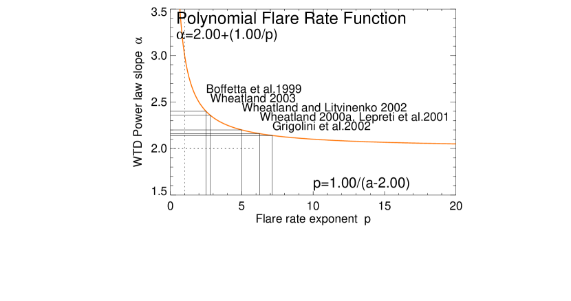
Figure 6: Inversion of the polynomial flare rate function exponents $p$ (x-axis) from the power law slope $\alpha$ (y-axis) of the theoretically predicted relationship $\alpha=2+1/p$.

Solar flare observations reveal a small range of power law slopes $\alpha\approx 2.1-2.4$ (Boffetta et al. 1999; Wheatland 2003; Wheatland and Litvinenko (2002), Wheatland 2000a; Lepreti et al. 2001; Grigolini et al. 2002; Aschwanden and McTiernan 2010), which map onto a polynomial exponent $p$ in the range of $p\approx 2.5-7.0$ (Fig. 6; Table 2). This range is expected since nonlinear processes require ($p\lower 1.72218pt\hbox{$\;\buildrel>\over{\scriptstyle\sim}\;$}2$).

3.6 Randomized Flaring

So far we modeled the time variability of the waiting time distribution on the largest scale of a full cycle, which has a typical time duration of $T\approx 11$ years, which we sampled with a time resolution of $dt=0.1$ year (or 36 days). In reality, however, there are temporal structures on much shorter time scales, down to $\tau\approx 1.0$ minute during episodes of high flaring activity, which strongly deviates from the slowly-varying solar cycle modulation of 11 years assumed in our previous modeling of the flare rate function $\lambda(t)$.

We perform an experiment of simulating the stochasticity of solar flare rates by random shuffling of the flare times $t_{i}$. The time profile $\lambda(t)$ shows a linear (positive) increase and a linear (negative) decrease in our first model (Fig. 7a). From this slowly-varying polynomial flare rate function with 24 time bins we shuffle some of the time bins arbitrarily, which mimics an irregular, stochastic, fast-varying flare rate function $\lambda(t)$ (Fig. 7b). As expected, the resulting waiting time distribution $N(\tau)$ reveals an identical power law slope, i.e., $\alpha\approx 2.2$ for both the slowly-varying and fast-varying polynomial functions over the duration of a solar cycle. This outcome is trivial, because it simply reflects the commutative property of arithmetic sums in linear algebra: The sum of the time-varying waiting time distributions is invariant to the time order. For instance, $\sum x_{1}+x_{2}+x_{3}=\sum x_{3}+x_{1}+x_{2}$, or any other permutation of values $x_{i}$. The commutative property simplifies our modeling enormously, since a simple monotonic increase of flare rates includes all possible permutations also.

A corollary of the communtative property is that the power law slope $\alpha$ is independent of the time duration of the observational sample or the time resolution, as long as the same range of flare rates is covered during the sample. Consequently, an observational sample may contain intermittent flaring of many short-duration flare bursts and still produce power law slopes of waiting times that are similar to those samples with a slowly-varying solar cycle profile. An illustration of a time profile containing multiple bursts is depicted in Fig. 7c, which again produces the same power law slope ($\alpha=2.23\pm 0.02$; Fig. 7f) as the entire solar cycle ($\alpha=2.23\pm 0.02$; Fig. 7d).

4 Discussion

4.1 Observational Constraints of Waiting Time Distributions

A comprehensive list of published waiting time distributions of solar flares has been presented in Table 1 of Aschwanden and Dudok de Wit (2021). In Table 2 of this study here we compile a subset of these observed waiting time distributions that cover at least a half solar cycle ($T/2\lower 1.72218pt\hbox{$\;\buildrel>\over{\scriptstyle\sim}\;$}5$ years), so that they contain the full flare rate variability from the solar minimum to the solar maximum (or vice versa). This selection criterion contains solar flares observed with the Hard X-ray Burst Spectrometer onboard the Solar Maximum Mission (HXRBS/SMM), the Rueven Ramaty High Energy Solar Spectrometric Imager (RHESSI), the Burst and Transient Source Experiment onboard the Compton Gamma Ray Observatory (BATSE/CGRO), the Geostationary Orbiting Earth Satellite (GOES), as well as coronal mass ejections observed with the Large Angle Solar Coronagraph onboard the Solar and Heliospheric Observatory (LASCO/SOHO). Large flare rate variability warrants power law functions for waiting time distributions, while insignificant flare rate variability renders exponential (stationary Poissonian) waiting time distributions.

What power law slopes $\alpha$ of waiting time distributions have been observed during full (or half) solar cycles ? As we show in Fig. 6, the combined range of observations narrows down to a relatively small range of power law slopes $\alpha_{obs}\approx 2.1-2.4$. These power law slopes $\alpha$ correspond to a range of $p\approx 2.5-7.0$ for the degree $p$ of the polynomial flare rate function (Fig. 6), according to the predicted relationship of $\alpha=2+1/p$ (Eq. 22). This means that the rise time of the flaring rate is not linear ($p\approx 1$), but rather is highly nonlinear ($p\lower 1.72218pt\hbox{$\;\buildrel>\over{\scriptstyle\sim}\;$}2$). Following this interpretation, all observed data sets are consistent with nonlinear behavior (Boffetta et al. 1999; Wheatland 2003, Wheatland and Litvinenko 2002; Wheatland 2000a; Lepreti et al. 2001; Grigolini et al. 2002). The nonlinear behavior is expected for solar flares because of its (nonlinear) avalanche-like growth characteristics that is typical for self-organized criticality models. The implication of this result stretches much further than to the rise time characteristics of the solar cycle, because it applies also to the average evolutionary behavior of many (clustered and intermittent) flare rate bursts, as depicted in Fig. (7c).

Interestingly, a power law slope of $\alpha=2.5$ has also been analytically derived for the case of the sinusoidal flare rate function, in terms of Bessel functions (Nurhan et al. 2021), which is identical to our derivation of the lower limit $\alpha\leq 2+1/p=2.5$ for nonlinear processes ($p\geq 2$). Theoretically, the power law slope is mostly determined by the behavior of the flare event rate function $\lambda(t)$ at the times with the slowest event rate, near $t=0$ and $t=T$, where $\lambda(t)\propto\sin{(\pi t/T)}^{2}$, and thus $\alpha=2+1/p=2.5$ for $p=2$.

4.2 Do Power Laws Exist ?

In this study we use numerical tools that can produce true random distributions of flare events (which should follow exponential functions with Poisson statistics), as well as non-stationary Poissonian distributions. The latter group produces more or less power law-like functions, but it has never been demonstrated whether we should expect an exact power law function. Since numerous deviations from exactly straight power law functions (in a log-N log-S histogram) have been noted before (Wheatland et al. 1998; Aschwanden and McTiernan 2010), some criticism has been raised whether power laws exist at all (Stumpf and Porter 2012). Here we have an answer that is summarized in Fig. 2. We calculated the analytical exact solution of a waiting time distribution for the linear case (with time evolution $\lambda(t)\propto t^{p}=t^{1}$, or $p=1$), which is derived in Appendix A, Eq. (A6). The solution contains terms of $\tau$, $\tau^{2}$, $\tau^{3}$, and $e^{-\tau}$, and therefore is of the type of an ideal power law function $\tau^{-\alpha}$ in the asymtotic limit only ($\lambda_{0}\tau\mapsto\infty$), where all other terms are exponentially small. A Pareto type-II function $(1+\tau)^{-\alpha}$ is a good approximation (Aschwanden and Dudok de Wit 2021; Aschwanden and McTiernan 2010; Aschwanden and Freeland 2012) that is accurate to first-order terms, but shows a gradual change in the power law slope with respect to the exact analytical solution. Moreover, in our numerical simulation of waiting time distributions we obtain a power law-like function too (Fig. 2), but the Poissonian weighting of a power law fit is biased towards the lower end (where the error bars are smallest and thus have the largest weight there). Thus, if a power law fit is obtained over the full inertial range, we predict that the average slope is slightly flatter than the asymptotic limit at the upper end, which is evident in the example shown in Fig. 2 (dashed line). Other examples are shown in Fig. 3, where deviations from ideal power laws show up clearly, since the non-stationary Poissonian model (with large time variability of the mean flare rate) predicts that a power law-like convolution consists of a superposition of multiple (but finite number) of exponential distributions. In summary, deviations from ideal power law functions are not significant for relatively small samples (with $N_{0}\approx 10^{1}-10^{3}$), but become significant for larger samples (with $N_{0}\lower 1.72218pt\hbox{$\;\buildrel>\over{\scriptstyle\sim}\;$}10^{4}$), as demonstrated in other works (Aschwanden 2015, 2019a, 2019b, Aschwanden and Dudok de Wit 2021), which are theoretically expected, and thus should be modeled correspondingly.

4.3 Self-Organized Criticality Models

After the previous disgression to previous observations and the discussion of whether power laws exist at all, let us come back to physical models that possibly could explain the observed power law slopes $\alpha$ of waiting time distributions.

Naively, to first order, one would expect that the distribution $N(\tau)$ is reciprocal to the mean waiting time, i.e., $N(\tau)\propto\tau^{-1}$, simply because the number of fragments is reciprocal to the length of a fragment in a one-dimensional “fragmentation” process. In other words, the product of the number $N$ multiplied with the duration of a time scale $T$ is invariant, i.e., $N_{T}\times T$ = const. However, this simplest model that predicts a scaling of $\tau^{-1}$ is not consistent with observations, which show distributions of $\approx\tau^{-2},...,\tau^{-3}$. It is likely that the one-dimensionality in the time domain is the culprit in this oversimplified model.

However, if we consider the generation of waiting times in the spatio-temporal domain, a spatial scale with length $L$ and time scale $T$ are required in a minimal model, which are coupled by the length scale distribution $N(L)dL$ and the transport equation $L(T)$. We can find such a model in the self-organized criticality concept, as briefly summarized in Section 2.5. Both relationships can be expressed with power laws, the scale-free size distribution of avalanches, $N(L)\ dL\propto L^{-d}dL$ (Eq. 26), and the diffusive transport mechanism, $L\propto T^{\beta/2}$ (Eq. 27), with $d=1,2,3$ the Euclidean dimension, and $\beta=1$ the classical transport coefficient. Taken these two relationships together, our SOC model predicts a power law distribution of flare durations $T$, i.e., $N(T)\propto T^{-\alpha}$, where the power law slope is defined as $\alpha=1+(d-1)\beta/2$ (Eq. 28). Thus, the SOC model predicts a value of $\alpha=2$ for the 3-D space geometry, while the values of $\alpha=1$ for 1-D and $\alpha=1.5$ for 2-D geometry are below the observed values, and thus can be ruled out. Interestingly, the predicted value of $\alpha=2.0$ for the 3-D world agrees with the independently calculated approximation of the Pareto type-II model (Eq. B2) in the asymptotic limit of $\tau\mapsto\infty$ (Eq. B3), which corroborates the SOC theory and the Pareto distribution function to some extent.

5 Conclusions

In this study we explore the origin of waiting time distribution functions, which provides a means to diagnose whether the events of a statistical distribution are produced by independent random events (obeying an exponential function) or by coherent clusters (obeying a power law function). This study is a follow-up on the pioneering work of Wheatland (2003) who concluded that non-stationary Poissonian processes produce power law-like distributions due to the (non-stationary) time variability of the mean flare rate. Although we find good agreement between the simulated and theoretically predicted parameters in the framework of non-stationary Poisson models postulated by Wheatland et al. (1998), the presented results do not rule out alternative interpretations, such as the nonlinear dynamics of MHD turbulence in active regions (Boffetta et al 1999; Carbone et al. 2002). Our findings and conclusions are briefly summarized in the following:

1. The theoretical calculation of a waiting time distribution function $N(\tau)\ d\tau$ represents a convolution of individual exponential distribution functions with a time-dependent flare rate function $\lambda(t)$. The flare rate function can be chosen arbitrarily, for which we choose polynomial, sinusoidal, and Gaussian functions (see 36 cases in Table 1), but we found that all three functions produce almost identical results, because their time variability is invariant to the multiplicity and temporal permutation of time structures.

2. New analytical solutions of the waiting time distribution function $N(\tau)d\tau$ have been found for polynomial flare rate functions $\lambda(t)\propto t^{p}$ in terms of the incomplete gamma function, as well as for the sinusoidal flare rate functions $\lambda(t)\propto\sin(t)^{2}$ in terms of Bessel functions (Nurham et al. 2021). Another useful approximation to polynomial flare rate functions is the Pareto type-II distribution function, $N(\tau)=N_{0}\left[1+c\tau/\alpha\right]^{-\alpha}$, with $\alpha=2+1/p$ being the (waiting time) power law slope.

3. The quadratic polynomial flare rate function, $\lambda(t)\propto t^{p}$, implies a high nonlinearity of degree $p\lower 1.72218pt\hbox{$\;\buildrel>\over{\scriptstyle\sim}\;$}2$ in the time variability of the flare rate. The nonlinear time variability applies theoretically to the long-duration variability of the solar cycle, but the real data reveal a high degree of intermittency, so that the nonlinear evolution applies to short-duration variability of active regions and to clustered flare burst episodes too.

4. We define a nonlinearity parameter $p$ (or degree of polynomial order) that characterizes the flare rate function $\lambda(t)\propto t^{p}$ in terms of its evolution, which has a theoretically predicted relationship of $\alpha\approx 2+1/p$ between the nonlinearity parameter $p$ and the waiting time power law slope $\alpha$. Thus we can predict the power law slope $\alpha$ as a function of the nonlinearity degree $p$. For instance, for linear processes ($p=1$) we expect a slope of $\alpha_{1}=3.0$, and likewise, for a nonlinear process ($p\approx 2$) we expect $\alpha_{2}=2.5$. Vice versa, we can predict the degree of nonlinearity $p$ from an observed waiting time power law slope $\alpha$, using the inverse relationship, $p=1/(\alpha-2)$.

5. A value of $\alpha=2+1/p$ has been predicted for the power law slope of waiting time distributions, based on analytical exact solutions in terms of the incomplete gamma function. The same value could be retrieved from the Pareto type-II distribution function. A fixed value of $\alpha=2.5$ has been obtained for the sinusoidal flare rate model (Nurhan et al. 2021), which is consistent with the nonlinear regime ($p\approx 2$) and would be expected for a process driven by the magnetic activity cycle of the solar dynamo. Another prediction of $\alpha=2$ has been derived from a self-organized criticality model, assuming a space-filling Euclidean dimension of ($D=3$) and classical diffusion as transport process ($\beta=1$), which occur, for instance, in chain reactions of solar flare avalanches. The agreement between the independent theoretical models corroborates our interpretation in terms of SOC models.

6. Do power laws exist ? This question is absolutely justified, as we demonstrate with three slightly different approximations in the case of waiting time distributions. Since a waiting time distribution of non-stationary Poissonian processes represents a superimposition of exponential functions, one can easily show deviations from ideal power laws. However, deviations from ideal power law functions are generally not significant for relatively small samples (with $N_{0}\approx 10^{2}-10^{3}$), but become significant for larger samples (with $N_{0}\lower 1.72218pt\hbox{$\;\buildrel>\over{\scriptstyle\sim}\;$}10^{4}$).

Future studies may investigate the predictions made for waiting time distributions by means of observational data sets, complementary to the numerical simulations demonstated here. It would be particulary important to test the clustering and sympathetic flaring on shorter time scales than the solar cycle examined here. A further benefit of this study is that the new analytic exact solutions for waiting time distributions, $N(\tau)d\tau$, could also be extended to occurrence frequency distributions of (flare) event durations, $N(T)\ dT$, which always exhibited larger deviations from strict power laws than the (flare) event size distributions, $N(S)\ dS$ (Bak et al. 1987, 1988).

APPENDIX A: Analytical Solution of Waiting Time Distribution for Case p=1

The waiting time distribution $N(\tau)\ dt$ of a Poissonian random process can be represented by an exponential distribution (Eq. 1) for the case of a stationary flare rate function $\lambda(t)=\lambda_{0}$. For a linearly increasing flare rate function $\lambda(t)=t/(T/2)$ (with $p=1$ in Eq. 9), the probability function is (Wheatland et al. 1998; Wheatland and Litvinenko (2002); Aschwanden and McTiernan (2010),

$$N(\tau)={\int_{0}^{T}\lambda(t)^{2}\exp{\left[-\lambda(t)\tau\right]}dt\over\int_{0}^{T}\ \lambda(t)\ dt}\ .$$

Inserting the flare rate function $\lambda(t)=\lambda_{0}({t/(T/2)})^{1}$ we obtain the integral,

$$N(\tau)={\int_{0}^{T/2}\lambda_{0}^{2}\left({t\over T/2}\right)^{2}\exp{\left[-\lambda_{0}\ \tau\ (t/(T/2))\right]}dt\over\int_{0}^{T/2}\lambda_{0}\left({t\over T/2}\right)dt}\ .$$

Substituting the variables $x=t/(T/2)$, $dt=(T/2)dx$, and $a=-\lambda_{0}\tau$, we obtain the integral,

$$N(\tau)={\int_{0}^{1}\lambda_{0}^{2}\ x^{2}\exp^{ax}dx\over\int_{0}^{1}x\ dx}\ ,$$

which has the analytical solution (Bronstein and Semendjajew 1960),

$$N(\tau)=\lambda_{0}\ \exp^{ax}\left({x^{2}\over a}-{2x\over a^{2}}+{2\over a^{3}}\right)_{x=0}^{x=1}$$

$$N(\tau)=2\lambda_{0}\exp^{a}\left[\left({1\over a}-{2\over a^{2}}+{2\over a^{3}}\right)-{2\over a^{3}}\right]\ ,$$

which can be expressed with $a=-\lambda_{0}\tau$ to show the explicit function of the waiting time $\tau$,

$$N(\tau)=2\lambda_{0}\left[{2\over\lambda_{0}^{3}\tau^{3}}-\exp^{-\lambda_{0}\tau}\left({1\over\lambda_{0}\tau}+{2\over\lambda_{0}^{2}\tau^{2}}+{2\over\lambda_{0}^{3}\tau^{3}}\right)\right]\ .$$

APPENDIX B: Pareto Type-II Approximation

An alternative generalization of a simple straight power law distribution function $N(\tau)\propto\tau^{-\alpha}$ is the Pareto Type-II distribution function, $N(\tau)\propto(1+\tau)^{-\alpha}$, which exhibits a power law-like function at large waiting times and becomes constant at small waiting times. Such a Pareto type-II function has been used previously to fit waiting time distributions (Aschwanden and McTiernan 2010; Aschwanden and Freeland 2012; Aschwanden and Dudok de Wit 2021). Here we present an analytical approximation of the waiting time distribution function.

We start with the expression of the waiting time distribution in terms of the gamma function (Eq. 23). In the asymptotic limit we have

$$N(\tau)\sim\lambda_{0}\ (\alpha-1)\Gamma(\alpha)\ (\lambda_{0}\tau)^{-\alpha}\ ,$$

where the slope $\alpha$ of the power law is (Eq. 22),

$$\alpha=2+{1\over p}\ .$$

This is also asymptotic to a Pareto type-II distribution of the form,

$$N_{P}(\tau)=\frac{N_{0}}{{\left(1+\frac{c\tau}{\alpha}\right)}^{\alpha}}\ .$$

Equating the two expression (Eq. B1) and (Eq. B2) yields,

$$N_{0}\left(\frac{\alpha^{\alpha}}{c^{\alpha}}\right)=\lambda_{0}\frac{(\alpha-1)\Gamma(\alpha)}{(\lambda_{0})^{\alpha}}\ .$$

Also, for a uniform approximation, we require that

$$N_{P}(0)=N_{0}(1-c\tau+...)$$

so that the constant $N_{0}$ is,

$$N_{0}=\lambda_{0}\left(\frac{p+1}{2p+1}\right)=\lambda_{0}\left(\frac{\alpha-1}{\alpha}\right)\ ,$$

which then yields the equivalence,

$$\lambda_{0}\left(\frac{\alpha-1}{\alpha}\right)\left(\frac{\alpha^{\alpha}}{c^{\alpha}}\right)=\lambda_{0}\frac{(\alpha-1)\Gamma(\alpha)}{(\lambda_{0})^{\alpha}}\ ,$$

and the constant $c$,

$$c=\frac{\alpha\lambda_{0}}{{\left(\alpha\Gamma(\alpha)\right)}^{1/\alpha}}$$

This theotetical solution has been checked numerically and compared with the exact solution based on the incomplete gamma function solution (Eq. 25), the asymptotic approximation, the Pareto distribution obtained from the power series, and the Pareto distribution obtained from the Padé approximation. The power series solution is inaccurate when $\lambda_{0}\tau>1$. The Padé approximation is reasonably accurate for all $\lambda_{0}\tau$ and matches the power law slope accurately.

APPENDIX C : Solution for Gaussian Event Rate Function

After we calculated exact solutions for the polynomial flare rate function $\lambda(t)$ (Section 2.4), while exact solutions for the sinusoidal flare rate are given in Nurhan et al. (2021), we derive here an approximate solution for the Gaussian flare rate also. The definition of the waiting time integral is (Eq. 10),

$$N(\tau)=\frac{\int_{0}^{T/2}\lambda^{2}(t)\exp(-\lambda(t)\tau)dt}{\int_{0}^{T/2}\lambda(t)dt}\ ,$$

where the Gaussian rate function is (Eq. 9),

$$\lambda(t)=\lambda_{0}\exp(-(t-T/2)^{2}/2\sigma^{2})\ .$$

We change the variables

$$y=(T/2-t)/\sqrt{2}\sigma\ ,$$

$$dy=-dt/\sqrt{2}\sigma\ ,$$

$$\lambda=\lambda_{0}e^{-y^{2}}\ ,$$

$$\beta=\frac{T}{2^{3/2}\sigma}\ ,$$

and obtain the waiting time integral in terms of the error function erf($\beta$),

$$N(\tau)=\lambda_{0}\frac{\frac{2}{\sqrt{\pi}}\int_{0}^{\beta}e^{-2y^{2}}\exp(-\lambda_{0}e^{-y^{2}}\tau)dy}{\frac{2}{\sqrt{\pi}}\int_{0}^{\beta}e^{-y^{2}}dy}=\lambda_{0}\frac{I(\tau,\beta)}{{\mathrm{e}\mathrm{r}\mathrm{f}}(\beta)}\ ,$$

where

$$I(\tau,\beta)=\frac{2}{\sqrt{\pi}}\int_{0}^{\beta}e^{-y^{2}}\exp(-\lambda_{0}e^{-y^{2}}\tau)dy\ ,$$

$${\mathrm{e}\mathrm{r}\mathrm{f}}(\beta)=\frac{2}{\sqrt{\pi}}\int_{0}^{\beta}\exp(-x^{2})dx\ ,$$

Now we have,

$$I(\tau,\beta)=\frac{1}{\lambda_{0}^{2}}\frac{d^{2}}{d\tau^{2}}\frac{2}{\sqrt{\pi}}\int_{0}^{\beta}\exp(-\lambda_{0}e^{-y^{2}}\tau)dy\ ,$$

We expand the exponential around $y=\beta$, as this will be the smallest value in the exponential and will dominate asymptotically.

$$e^{-y^{2}}=e^{-\beta^{2}}(1-2\beta(y-\beta)+...)\ ,$$

Consequently we obtain,

$$\int_{0}^{\beta}\exp(-\lambda_{0}e^{-y^{2}}\tau)dy\sim\int_{\beta-\epsilon}^{\beta}\exp(-\lambda_{0}\tau e^{-\beta^{2}}(1+2\beta(\beta-y))dy=\exp(-\lambda_{0}\tau e^{-\beta^{2}})\int_{0}^{\epsilon}\exp(-2\lambda_{0}\tau\beta e^{-\beta^{2}}q)dq\ ,$$

which introduces only an exponenitally small error, so that we can now take $\epsilon\to\infty$,

$$\int_{0}^{\beta}\exp(-\lambda_{0}e^{-y^{2}}\tau)dy\sim\frac{\exp(-\lambda_{0}\tau e^{-\beta^{2}})}{2\lambda_{0}\tau\beta e^{-\beta^{2}}}\ .$$

Taking the leading order terms,

$$-\frac{d}{d\tau}\frac{\exp(-\lambda_{0}\tau e^{-\beta^{2}})}{2\lambda_{0}\tau\beta e^{-\beta^{2}}}=\frac{\exp(-\lambda_{0}\tau e^{-\beta^{2}})}{2\beta\tau}\left(1+\frac{1}{\lambda_{0}\tau e^{-\beta^{2}}}\right)\ ,$$

$$\frac{d^{2}}{d\tau^{2}}\frac{\exp(-\lambda_{0}\tau e^{-\beta^{2}})}{2\lambda_{0}\tau\beta e^{-\beta^{2}}}=\frac{\lambda_{0}e^{-\beta^{2}}\exp(-\lambda_{0}\tau e^{-\beta^{2}})}{2\beta\tau}\left(1+\frac{2}{\lambda_{0}\tau e^{-\beta^{2}}}+O{\left(\frac{1}{\lambda_{0}\tau}\right)}^{2}\right)\ ,$$

and then obtain,

$$N(\tau)\sim\lambda_{0}\frac{e^{-\beta^{2}}\exp(-\lambda_{0}\tau e^{-\beta^{2}})}{\sqrt{\pi}\beta\lambda_{0}\tau~{}{\mathrm{e}\mathrm{r}\mathrm{f}(\beta)}}\left(1+\frac{2}{\lambda_{0}\tau e^{-\beta^{2}}}\right)\ .$$

In the $\delta$-function limit we have $\sigma\to 0$ and $\beta\to\infty$, so that the second term in the expansion will dominate and $\alpha=2$, consistent with the $\delta$-function limit we have seen as $p\to\infty$ in the polynomial case. Comparing with the numerical solution, it is apparent that a power-like form is found for $\lambda_{0}\tau\approx 5-10$ and does not apply at larger values of $\tau$. Note that power laws are generally substantially different as $\sigma$ varies.

Acknowledgements: We acknowledge valuable discussions with Dudok de Wit. Part of the work was supported by NASA contracts NNG04EA00C and NNG09FA40C. JRJ and YIN acknowledge NASA grant NNX16AQ87G.

References

Aschwanden, M.J. and McTiernan, J.M. 2010, ApJ 717, 683

Aschwanden, M.J. 2011 Self-Organized Criticality in Astrophysics. The Statistics of Nonlinear Processes in the Universe, Springer-Praxis: New York, 416p.

Aschwanden, M.J. 2012, A&A 539:A2

Aschwanden, M.J. and Freeland, S.M. 2012, ApJ 754:112

Aschwanden, M.J. 2014, ApJ 782, 54

Aschwanden, M.J. 2015, ApJ 814:19

Aschwanden, M.J., Crosby, N., Dimitropoulouy, M., et al. 2016, SSRv 198:47

Aschwanden, M.J. 2019a, ApJ 880, 105

Aschwanden, M.J. 2019b, ApJ 887:57

Aschwanden, M.J. and Dudok de Wit, T. 2021, ApJ 912:94

Bak, P., Tang, C., and Wiesenfeld, K. 1987, Physical Review Lett. 59/27, 381

Bak, P., Tang, C., and Wiesenfeld, K. 1988, Physical Rev. A 38/1, 364

Bauke, H. 2007, Eur.Phys.J.B. 58, 167

Boffetta, G., Carbone, V., Giuliani, P., Veltri, P., and Vulpiani, A. 1999, Phys.Rev.Lett. 83, 4662

Bourouaine, S., Perez, J.C., Klein, K.C., Chen, C.H.K. 2020, ApJ 904, 308

Carbone, V., Cavazzana, R., Antoni, V., Sorriso-Valvo, L. et al. 2002, Europhysics Letters 58/3, 349

Cheng, Y., Zhang, G.Q., and Wang,F.Y. 2020, MNRAS 491, 1498

Bronstein, I.N. and Semendjajev, A.K. 1960, Harry Deutsch: Zürich

Dudok de Wit, P., Krasnoselskikh, V.V., Bale, S.D., et al. 2020, ApJSS 246:39

Eastwood, J.P., Wheatland, M.S., Hudson, H.S., et al. 2010, ApJ 708, L95

Grandell, J. 1997, Mixed Poisson Processes, Chapman and Hall: London

Greco, A., Matthaeus, W.H., Servidio, S., Chuychai, P. and Dmitruk, P. 2009, ApJ 2, L111

Goldsteinm, M.L., Morris, S.A., and Yen, G.G. 2004, Eur.Phys.J.B. 41, 255

Gorobets, A. and Messerotti, M. 2012, SoPh 281, 651

Grigolini, P., Leddon,D., and Scafetta,N. 2002, Phys.Rev.Lett E, 65/4. id. 046203

Guidorzi,C., Dichiara, S., Frontera,F., et al. 2015, ApJ 801, 57

Hawley, S.L., Davenport, J.R.A., Kowalski, A.F., Wisniewski, John P. et al. 2014, ApJ 797, 12H

Hudson, H.S. 2020, MNRAS 491 4435

Kingman J.F.C. 1993, Poisson Processes, Oxford University Press

Leddon, D. 2001, eprint arXiv:cond-mat/0108062, Dissertation Abstracts International, Volume: 63-12, Section: B, page: 5891; 56 p.

Lepreti, F., Carbone, V., and Veltri,P. 2001, ApJ 555, L133

Li,C., Zhong, S.J., Xu, Z.G., et al. 2018, MNRAS 479 L139

Melatos, A., Peralta, C., and Wyithe, J.S.B. 2008, ApJ 672:1103

Melatos, A., Howitt, G. 2018, ApJ 863, 196

Morales, L.F. and Santos, N.A. 2020, SoPh 295, 155

Newman, M.E.J. 2005, Contemp.Phys. 46, 323

Norman, J.P., Charbonneau, P., McIntosh, S.W., and Liu, H. 2001, ApJ 557, 891

Nurhan, Y.I., Johnson, J.R., Homan, R., et al. (2021), GRL, (subm.)

Sanchez,R., Newman, D.E., Ferenbaugh, W., et al. 2002, Phys.Rev E 66, 036124

Streit, R.L. 2010, Poisson Point Processes, Springer: New York

Li, C., Zhong, S.J., Wang, L., et al. 2014, ApJ 792, L26

Snelling, J.M., Johnson, J., Willard, J. et al. 2020, ApJ 869, 148

Stumpf, M.P.H. and Porter, M.A. 2012, Science 335, 10 Feb 2012

Uritsky, V.M., Paczuski, M., Davila, J.M., and Jones, S.I. 2007, Phys. Rev. Lett. 99, 025001

Usoskin, I.G., Solanki, S.K., and Kovaltsov, G.A. 2007, A&A 471, 301

Wang, Y., Liu, L., Shen, C., et al. 2013, ApJ 763, L43

Wang, F.Y., Dai, Z.G., Yi, S.X., and Xi, S.Q. 2015, ApJS 216, 8

Wang, J.S., Wang, F.Y., and Dai, Z.G. 2017, MNRAS 471 2517

Wanliss, J.A. and Eygand, J.M. 2007, GRL 34, 4107

Wheatland, M.S., Sturrock,P.A., and McTiernan,J.M. 1998, ApJ 509, 448

Wheatland,M.S. 2000a, ApJ 536, L109

Wheatland,M.S. 2000b, SoPh 191, 381

Wheatland, M.S. 2001, SoPh 203, 87

Wheatland, M.S. and Litvinenko, Y.E. 2002, SoPh 211, 255

Wheatland, M.S. 2003, SoPh 214, 361

Wheatland, M.S. 2004, ApJ 609, 1134

Wheatland, M.S., and Craig, I.J.D. 2006, SoPh 238, 73

Yeh, C.T., Ding, M., and Chen, P. 2005, ChJAA 5, 193

Yi, S.X., Xi, S.Q., Yu, Hai et al. 2016, ApJS 224, 20

Table 1: Power law slopes $\alpha$ of waiting time distributions, calculated by numerical simulations for three model types (polynomial, sinusoidal, Gaussian), as a function of the model exponent $p$. The theoretically predicted slope is $\alpha=2+1/p$.

p	$\alpha_{P}$	$\alpha_{S}$	$\alpha_{G}$	$\alpha_{theo}$
	Polynomial	Sinusoidal	Gaussian	2+1/p
0.5	3.25	3.39	3.48	4.00
1.0	2.99	3.02	2.98	3.00
1.5	2.60	2.90	2.55	2.67
2.0	2.51	2.61	2.34	2.50
2.5	2.32	2.59	2.34	2.40
3.0	2.30	2.56	2.33	2.33
3.5	2.27	2.39	2.33	2.29
4.0	2.25	2.39	2.33	2.25
4.5	2.24	2.40	2.33	2.22
5.0	2.15	2.40	2.24	2.20
5.5	2.14	2.39	2.24	2.18
6.0	2.13	2.37	2.25	2.17

Table 2: Waiting time distributions measured from solar flares over at least a half solar cycle ($T\lower 1.72218pt\hbox{$\;\buildrel>\over{\scriptstyle\sim}\;$}5$ years).

Observations	Observations	Number	Waiting	WTD	Powerlaw	References
year of events	spacecraft or	range	time
	instrument		$\tau$		$\alpha_{\tau}$
1980-1989	HXRBS/SMM	12,772	$0.01-500$ hrs	PL	$\approx 2.0$	Aschwanden & McTiernan (2010)
2002-2008	RHESSI	11,594	$2-1000$ hrs	PL	$\approx 2.0$	Aschwanden & McTiernan (2010)
1991-2000	BATSE/CGRO	7212	$1-5000$ hrs	PL	$2.14\pm 0.01$	Grigolini et al. (2002)
1975-1999	GOES 1-8 A	32,563	$1-1000$ hrs	PL	$2.4\pm 0.1$	Boffetta et al. (1999)
1975-1999	GOES 1-8 A	32,563	$1-1000$ hrs	PL	$2.16\pm 0.05$	Wheatland (2000a), Lepreti et al. (2001)
1975-2001	GOES 1-8 A	…	$1-1000$ hrs	PL	$2.2\pm 0.1$	Wheatland and Litvinenko (2002)
1996-2001	SOHO/LASCO	4645	$1-1000$ hrs	PL	$2.36\pm 0.11$	Wheatland (2003)

Figure 1: Parameter range of polynomial flare rate functions $\lambda(t)$ for exponents $p=0.1,...,10$, including the linear case $p=1$ for $\lambda(t)\propto t$, or the nonlinear (quadratic) case $p=2$ for $\lambda(t)\propto t^{2}$.

Figure 2: Comparison of three different calculation methods of the waiting time distribution function: Monte Carlo simulation (histogram) with power law fit (dashed curve), analytical exact solution (thick solid curve), and Pareto approximation (thin solid curve). The fitting range is defined by the inertial range $[x_{0},x_{2}]$. The ratio of the slopes $\alpha_{exact}/\alpha_{fit}=1.12$ is attributed to the Poissonian weighting bias.

Figure 3: Six cases of numerical simulations of the waiting time distributions with different time resolutions dt=(1 year)/$n_{bin}$, $n_{bin}=1,2,4,8,16,32$. The waiting time components are shown individually for each bin (dashed curves in right panels), which sum up to the total (histograms in right panels). Note that the power law slope is almost constant and thus independent of the the time resolution. The theoretical slope of a continuous sinusoidal model with $\lambda(t)\propto\sin{(t)}^{2}$ with exponent $p=2$ is $\alpha=2+1/p=2.5$ agrees well with the simulations with $\alpha\approx 2.4-2.6$.

Figure 7: Comparison of three different flare rate functions $\lambda(t)$: (a) polynomial (linear) function, (b) flucutations simulated by random shuffling of time bins, and (c) flare clustering. Note that the wait time distribution has near identical values ($\alpha\approx 2.1-2.2$) due to the commutativity in summing the flare rates from different time bins. The power law slope values are not corrected for the Poissonian weighting bias.