Advanced modeling of materials with PAOFLOW 2.0:
New features and software design

Abstract

Recent research in materials science opens exciting perspectives to design novel quantum materials and devices, but it calls for quantitative predictions of properties which are not accessible in standard first principles packages. PAOFLOW  is a software tool that constructs tight-binding Hamiltonians from self-consistent electronic wavefunctions by projecting onto a set of atomic orbitals. The electronic structure provides numerous materials properties that otherwise would have to be calculated via phenomenological models. In this paper, we describe recent re-design of the code as well as the new features and improvements in performance. In particular, we have implemented symmetry operations for unfolding equivalent k-points, which drastically reduces the runtime requirements of first principles calculations, and we have provided internal routines of projections onto atomic orbitals enabling generation of real space atomic orbitals. Moreover, we have included models for non-constant relaxation time in electronic transport calculations, doubling the real space dimensions of the Hamiltonian as well as the construction of Hamiltonians directly from analytical models. Importantly, PAOFLOW has been now converted into a Python package, and is streamlined for use directly within other Python codes. The new object oriented design treats PAOFLOW’s computational routines as class methods, providing an API for explicit control of each calculation.

1 Introduction

Exploring phenomena and properties of novel materials requires accurate and efficient computational tools that can be easily customized and manipulated. In this context, ab initio tight-binding (TB) Hamiltonians constructed from self-consistent quantum-mechanical wavefunctions projected onto a set of atomic orbitals have been very successful, since they allow calculations for materials that cannot be properly addressed using only density functional theory (DFT) such as large moiré superstructures or properties of exotic quantum systems where spin and topology play an important role. PAOFLOW  [1] is a new software tool that employs an efficient procedure of projecting the full plane-wave solution on a reduced space of pseudoatomic orbitals [2, 3], and provides an interpolated electronic structure to promptly compute a plethora of relevant quantities, including optical and magnetic properties, charge and spin transport as well as topological invariants. Importantly, in contrast with other common approaches the projection does not require any additional inputs and can be successively integrated in high-throughput calculations of arbitrary complex materials. The code has been employed in multiple areas of materials science since its initial release in 2016. In particular, several groups used it to compute the (spin) Berry curvature as well as spin and/or anomalous Hall conductivity (SHC and AHC) in a variety of materials, ranging from $\beta$-W to magnetic antiperovskites [7, 4, 5, 6, 8]. Transport quantities, such as the electrical and thermal conductivity, were also computed in order to analyze carrier mobility in thermoelectrics [9, 10].

The software package has recently undergone a major refactor, resulting in a large variety of properties that can be calculated as well as highly improved performance. Many improvements were made to simplify the user experience, to make the package more modular, and to create an API for manipulating TB Hamiltonians. PAOFLOW, now installed as a Python package, features an object oriented design and contains an importable PAOFLOW class, allowing multiple Hamiltonians to be constructed and manipulated simultaneously. This framework enables high-throughput materials analysis within a single python file. While explicit descriptions of the code’s methodology are available in the original PAOFLOW paper [1], in this paper we outline PAOFLOW’s modified features, detail new functionalities, and provide a user manual for operating the various methods available within the package. Currently, PAOFLOW is publicly available under the terms of the GNU General Public License as published by the Free Software Foundation, either version 3 of the License, or any later version. It is also integrated in the AFLOW${{{{\pi}}}}$ high-throughput framework [11] and distributed at http://www.aflow.org/src/aflowpi and http://www.aflow.org/src/paoflow [12, 13].

2 Installation and software design

PAOFLOW is written in Python 3.8 (using the Python standard libraries, NumPy and SciPy). Parallelization on CPUs uses the openMPI protocol through the mpi4py module. The PAOFLOW package can be easily installed on any hardware. Installation directly from the Python package index (PyPi) is possible with the single command: pip install paoflow. Otherwise, one may clone the PAOFLOW repository from GitHub and install it from the root directory with the command: python setup.py install. The package requires no specific setup, provided that the prerequisite Python 3.8 modules are installed on the system. Example codes illustrating PAOFLOW’s capabilities are included on GitHub, in the examples/ directory of the PAOFLOW repository. Once installed, PAOFLOW can be imported into any Python code and used in conjunction with other software packages. It should be noted that, in PAOFLOW 1.0 two control files were required: main.py to begin the execution, and inputfile.xml to provide details of the calculation. In PAOFLOW 2.0 the desired routines are called directly from the Python code, eliminating the need for inputfile.xml. To facilitate the transition between the versions, in the examples/ directory we have provided an updated main.py file which allows use of the version 1.0 XML inputfile structure in PAOFLOW 2.0.

Generally, PAOFLOW requires a few basic calculations performed with the Quantum ESPRESSO (QE) package [14]. The first (self-consistent) run generates a converged electronic density and Kohn-Sham (KS) potential on an appropriate Monkhorst and Pack (MP) k-point mesh (pw.x). The second (non self-consistent) one (pw.x) evaluates eigenvalues and eigenfunctions on a larger MP mesh and often for an increased number of bands. In PAOFLOW 1.0 the latter required full k-point mesh without using symmetries, i.e. setting flags nosym=.true. and noinv=.true. in QE inputfile, while version 2.0 can reconstruct equivalent k-points from symmetry operations and has no such requirement, which greatly reduces the computation time at the level of DFT. As a next step, the KS wavefunctions from QE must be projected onto PAO basis functions. Also here we have introduced an important change - a new capability is the generation of real space atomic orbitals, constructed from the product of radial components from pseudopotential files and spherical harmonics specifying angular momentum dependence. The user can thus choose between two different options: project the KS wavefunctions onto this internally constructed PAO basis set (Sec. 3.2), or post-processing the QE output with projwfc.x in order to perform the projection, as it was done in version 1.0. If the projections are computed using QE, the eigenfunctions must be read by PAOFLOW before the construction of a PAO Hamiltonian (Sec. 3.3). Finally, PAOFLOW 2.0 introduces a possibility to operate with no preprocessing requirements from QE, where built-in or user-defined models serve as the recipe for building Hamiltonians. Implementing these models requires specific information about the atomic system a priori, and their usage is described in Section 4.

Central to PAOFLOW 2.0 is an internal object called the DataController, which has the sole responsibility of collecting and maintaining important information about the atomic system and its corresponding Hamiltonian. The DataController is initially populated with data from the QE calculation, providing many of PAOFLOW’s routines with required information and simplifying the way of calling functions by the user. Moreover, the DataController saves quantities needed for subsequent calculations, such as the Hamiltonian’s gradient or the adaptive smearing parameters. In fact, many routines require calculation of some quantities as a prerequisite. For example, the spin_Hall routine requires the Hamiltonian’s gradient, which means that the gradient_and_momenta should be called first to populate the DataController with the gradient and momenta. The DataController stores the system information in two dictionaries: one for strings and scalar attributes (data_attributes) and another for vector and tensor quantities (data_arrays). Such a structure allows computed quantities to be easily accessed from PAOFLOW and utilized in customized calculations defined by the user. Note that the dictionary keys are consistent with the naming conventions of PAOFLOW 1.0 to facilitate backwards compatibility with the XML inputfiles and minimize differences in the user experience when transitioning from the previous version.

3 Code description and package usage

PAOFLOW’s most fundamental procedure is the construction of accurate PAO Hamiltonians, and the code’s object-oriented design allows users to manipulate multiple Hamiltonians easily. A PAOFLOW object is responsible for a single Hamiltonian, which is constructed and operated on with PAOFLOW’s class methods. If instead of DFT electronic wavefunctions a TB model is used to construct the Hamiltonian, the new PAOFLOW object will create the Hamiltonian immediately. Otherwise, the KS wavefunctions are read from the output of QE. The atomic orbitals are constructed and the KS wavefunctions are projected onto them with the projections routine, creating the PAO basis. If the projections are performed by QE’s module projwfc.x, they must be read explicitly with read_atomic_proj_QE. Then, the Hamiltonian is constructed with build_pao_hamiltonian, which allows PAOFLOW’s other class methods to become functional. Listing 1 provides an example source code for building the PAOFLOW object, reading projections performed by QE, and constructing the PAO Hamiltonian. Listing 2 performs the same initialization procedure, but uses the internal atomic orbital projection scheme. An ellipsis appearing in any listing indicates that other PAOFLOW routines may follow.

The following subsections outline PAOFLOW’s individual routines and the arguments that they accept for control. These routines belong to the file PAOFLOW.py, located in the package’s src/ directory, and should be called directly by the user.

3.1 The constructor: PAOFLOW

The PAOFLOW constructor acquires information about the python execution, the names of input/output/working directories, and about the atomic system. It builds and populates the DataController, which will maintain the important quantities involved in calculations, handle communication in multi-core runs, and write files to disc when necessary.

For PAOFLOW to build a Hamiltonian, the constructor must be passed data with either the location of Quantum ESPRESSO’s .save directory or required specifications for an analytical TB model. The QE .save directory contain up to two files from the execution of QE: data-file-schema.xml (data-file.xml in previous versions of QE) generated by the main run with pw.x, and atomic_proj.xml generated by the post-processing tool projwfc.x, if the projections are computed with QE. To implement a TB model from scratch, rather than starting from the KS wave function solutions of DFT, a dictionary containing the model’s label and other required parameters should be passed into the model argument (see Section 4).

Arguments for the constructor, PAOFLOW:

• workpath (string) - Default: ’./’ - Path to the working directory. Defaults to the current working directory.

• outputdir (string) - Default: ’output’ - Name of the directory to store output data files. The directory is created automatically in the workpath, if it does not already exist.

• inputfile (string) - Default: None - This argument is primarily for backwards compatibility with PAOFLOW 1.0. It names the XML inputfile with control parameters described in Ref. [1]. The XML inputfile provides also a consistent descriptor format for highly automated calculations, utilized by AFLOW$\pi$.

• savedir (string) - Default: None - Name of the Quantum ESPRESSO .save directory, relative to the working directory.

• model (dict) - Default: None - Dictionary specifying parameters required to implement a TB model. See Section 4.

• npool (integer) - Default: 1 - Number of batches to process when communicating between processors. This value will be automatically increased if the Hamiltonian size exceeds mpi4py’s limit for a single cross core message.

• smearing (string) - Default: ’gauss’ - Selects the broadening technique used to smooth computed quantities. Options include ’gauss’, ’m-p’ (Methfessel-Paxton), and None.

• acbn0 (bool) - Default: False - Read overlaps to construct a non-orthogonal PAO Hamiltonian. Necessary to perform ACBN0 calculations [15, 16].

• verbose (bool) - Default: False - Flag for high verbosity. Set True to include additional information in the PAOFLOW output.

• restart (bool) - Default: False - Indicates the continuation of a previous run from the saved state. Once the PAOFLOW object is instantiated, the restart_load routine should be called with the save file’s prefix as an argument. An example is provided in listings 4 and 5.

3.2 projections

Perform projections of the KS eigenfunctions onto the pseudoatomic orbital basis which is constructed by PAOFLOW based on the information in the atomic pseudopotential files. This operation requires that PAOFLOW is instantiated by passing a QE .save directory with required XML file from the self-consistent and non self-consistent calculations. Listing 2 provides example usage of the projections routine, and a complete description of the projection methodology can be found in the Appendix of Ref. [2].

3.3 read_atomic_proj_QE

Read the projections of KS wavefunctions onto the atomic orbital basis of the pseudopotential, performed by the QE routine projwfc.x and written to atomic_proj.xml. Any time that the Hamiltonian is built directly from the projections of QE, this routine should be called immediately after the constructor.

read_atomic_proj_QE does not accept any arguments.

3.4 projectability

The projectability routine determines which bands do not meet projectability requirements, flagging them for shift into the null space. The projectability $p_{\bf k}$ is a quantity measuring how well a KS Bloch state is represented by orbitals of the PAO basis, as described in Section 3 of Ref. [1]. If $p_{\bf k}\approx 1$, the PAO basis set accurately represents that particular Bloch state for ${\bf k}$. $p_{\bf k}\ll 1$ indicates that the state is poorly represented and should be excluded. The projection threshold pthr selects the minimum allowed projectability for accepting a band. All bands which do not meet the criteria are projected to the null space during the Hamiltonian’s construction, in one of two ways. Either as

$$\hat{H}(\mathbf{k})=AEA^{\dagger}+\kappa\left(I-AA^{\dagger}\right)$$ (1)

following Ref. [17] or

$$\hat{H}(\mathbf{k})=AEA^{\dagger}+\kappa\left(I-A\left(A^{\dagger}A\right)^{-1}A^{\dagger}\right)$$ (2)

according to Ref. [2]. Unless the shift argument is explicitly set to a floating point value, the shifting parameter $\kappa$ is determined automatically by this routine. Which method is used to remove low-projectability bands during the Hamiltonian construction is selected by argument shift_type, in the pao_hamiltonian routine (Sec. 3.5).

Arguments for projectability:

• pthr (float) - Default: 0.95 - The projectability threshold. All bands with a minimum projectability of the pthr value or higher are included in the Hamiltonian.

• shift (string or float) - Default: ’auto’ - Float to indicate the value (in eV) of the null space cutoff ($\kappa$ in eqs. 1 and 2). Bands beneath the projectability threshold will be shifted to this value. Providing the default argument ’auto’ automatically sets shift’s value to the minimum energy of the first band that fails the projectability threshold.

3.5 pao_hamiltonian

This routine constructs the Hamiltonian in both real space and momentum space. After this routine is completed, the data controller will contain arrays HRs and Hks, for the respective real space and k-space Hamiltonians.

Arguments for pao_hamiltonian:

• shift_type (integer) - Default: 1 - Determines which method (Eq. 2 by default) is used to remove bands into the null space.
  0 - Eq. 1, 1 - Eq. 2, or 2 - No shift.

• insulator (bool) - Default: False - Setting this flag as True asserts that the system is insulating, setting the top of the highest occupied band to 0 eV. The Fermi energy is calculated for metallic systems, which corrects numerical discrepancies from the projection routine and irreducible wedge unfolding. This flag is set True automatically if the QE ouput does not contain smearing parameters.

• write_binary (bool) - Default: False - Flag to write the files necessary for the ACBN0 routine [18]. Overlaps from projwfc.x are required from prerequisite QE calculations, and this flag is required for further use with ACBN0.

• expand_wedge (bool) - Default: True - Applies symmetry operations to the k-mesh unfolding the irreducible wedge into the complete Brillouin zone, and evaluates the Hamiltonian matrix elements for every k-point. PAOFLOW routines act on the full grid of k-points (True), while ACBN0 only requires the irreducible wedge (False).

• symmetrize (bool) - Default: False - The Hamiltonian incurs numerical errors during the process of unfolding the wedge. Certain routines, such as find_weyl_points, are sensitive to the Hamiltonian’s symmetric components. Setting this flag to True symmetrizes the Hamiltonian with an iterative procedure to reduce numerical errors in the Hamiltonian’s symmetry.

• thresh (float) - Default: 1e-6 - The tolerance of symmetrization, if the procedure is performed.

• max_iter (integer) - Default: 16 - The maximum number of iterations that the symmetrization procedure will perform.

3.6 bands

Computes the band structure along the AFLOW standard path for the specified Bravais lattice. Alternatively, a custom path can be created by defining the high symmetry points in a dictionary and the band path as a string (see Listing 2). The path is Fourier interpolated to an arbitrary resolution, controlled by argument nk.

Arguments for bands:

• ibrav (integer) - Default: None - The Bravais lattice identifier, as specified by Quantum ESPRESSO.

• band_path (string) - Default: None - String of high symmetry point labels separated by ’-’ for a line connecting two points or ’|’ to place the points directly adjacent on the path (see Listing 2). If band_path is None the standard AFLOW path will be used [19].

• high_sym_points (dictionary) - Default: None - A dictionary mapping the string label of a high symmetry point to its three-dimensional crystal coordinate. (Listing 2)

• fname (string) - Default: ’bands’ - File name prefix for the bands. One file is written for each spin component (see listing 2).

• nk (int) - Default: 500 - Number of points to compute along the band path.

3.7 interpolated_hamiltonian

Fourier interpolation of the PAO Hamiltonian can increase the k-grid to an arbitrary density, as described and illustrated in the manuscript for PAOFLOW 1.0. The new desired dimension should be specified for nk1, nk2, and nk3. The default behaviour is to double the original nk dimension of any unspecified nfft argument. This routine populates the DataController with a new array ’Hksp’, the interpolated Hamiltonian.

Arguments for interpolated_hamiltonian:

• nfft1 (integer) - Default: None - The desired new dimension for the Hamiltonian’s previous dimension nk1. The nfft dimension should be greater than or equal to the previous nk dimension. If no argument is provided the original k-grid dimension is doubled.

• nfft2 (integer) - Default: None - New interpolated dimension for nk2, following the same scheme as nfft1.

• nfft3 (integer) - Default: None - New interpolated dimension for nk3, following the same scheme as nfft1 and nfft2.

• reshift_Ef (bool) - Default: False - Shift the Hamiltonian’s diagonal elements such that zero lies at the recomputed Fermi energy or at the top of the valence band.

3.8 spin_operator

The spin operator plays important role in several calculations performed by the PAOFLOW code. Generally, when the spin operator ${\bf S}_{j}$ is required, PAOFLOW automatically constructs it. However, ${\bf S}_{j}$ can be explicitly computed by calling this routine. The shell levels and their occupations are automatically read from pseudopotentials in the .save directory.

Arguments for spin_operator:

• spin_orbit (bool) - Default: False - Set this flag to True if spin orbit coupling is added at the PAO level (with the adhoc_spin_orbit routine).

3.9 add_external_fields

PAOFLOW supports the addition of electric fields, onsite Zeeman fields, or Hubbard corrections directly to the PAO Hamiltonian [20, 15]. Fields must be added after the Hamiltonian’s construction. Listing 3 provides an example where an electric field and Hubbard correction are simultaneously added to a Hamiltonian.

Arguments for add_external_fields:

• Efield (ndarray or list) - Default: [0.] - An array of the form [$E_{x}$,$E_{y}$,$E_{z}$], added to the diagonal elements of the Hamiltonian. Listing 3 provides an example of adding an electric field with one non-zero component.

• Bfield (ndarray or list) - Default: [0.] - An array of the form [$B_{x}$,$B_{y}$,$B_{z}$], specifying the strength and direction of an on-site magnetic field.

• HubbardU (ndarray or list) - Default: [0.] - An array with one U entry for each orbital, e.g. [$U_{1}$,$U_{2}$,…,$U_{n}$] where $n$ is the number of orbitals. An example is provided in Listing 3.

3.10 adhoc_spin_orbit

This routine allows the addition of spin-orbit coupling (SOC) at the PAO level. SOC is implemented for the following shell configurations, provided as the orb_pseudo argument: s, sp, spd, ps, ssp, sspd, & ssppd.

Arguments for adhoc_spin_orbit:

• naw (ndarray or list) - Default: [1] - List containing the number of wave functions for each pseudopotential.

• phi (flaot) - Default: 0. - Spin orbit azimuthal angle.

• theta (float) - Default: 0. - Spin orbit polar angle.

• lambda_p (ndarray or list) - Default: [0.] - Array of p-orbital coupling strengths.

• lambda_d (ndarray or list) - Default: [0.] - Array of d-orbital coupling strengths.

• orb_pseudo (list) - Default: [’s’] - List of strings, containing the orbital configuration for each pseudopotential.

3.11 doubling_Hamiltonian

Doubles the real space dimensions of the Hamiltonian, creating a supercell in any desired direction. Naturally, the number of wavefunctions in the Hamiltonian increases by a factor $2^{\bf nx}\times 2^{\bf ny}\times 2^{\bf nz}$. Doubling is performed one time in each dimension by default, and doubling can be suppressed by setting the argument for a dimension to 0.

Arguments for doubling_Hamiltonian:

• nx (int) - Default: 1 - Number of times to double the x dimension. If nx is set to 2 the resulting cell is 4 times larger in the x direction.

• ny (int) - Default: 1 - Number of times to double the y dimension.

• nz (int) - Default: 1 - Number of times to double the z dimension.

3.12 topology

The topology routine calculates various quantities along the AFLOW standard k-path. If the user generates a custom path with bands, prior to this routine, this path will be used when calculating the Z2 invariance and topological properties.

Arguments for topology:

• eff_mass (bool) - Default: False - Setting this flag True computes the Hamiltonian’s second derivative along the k-path. The effective mass is calculated and saved to file with naming convention effmass_IJ_S.dat. The indices I and J are specified by the arguments ipol and jpol. Index S is specified by spin polarization at the DFT level.

• Berry (bool) - Default: False - Set True to calculate the Berry curvature along the k-path and writes results to file as Omega_IJ.dat. Here, I and J are indices of the Berry curvature ($\Omega_{ij}$) and are specified by ipol and jpol respectively.

• spin_Hall (bool) - Default: False - Setting True calculates the spin Berry curvature ($\Omega^{s}_{ij}$) along the k-path and writes the results to files Omegaj_S_IJ.dat. Here, the indices I, J, and S are specified by the arguments ipol, jpol, and spol. This routine automatically computes the Berry curvature, but no files for Berry are written unless its flag is explicitly set True.

• spol (integer) - Default: None - Spin polarization index of the spin Berry curvature calculation. This selects which component of the spin operator is used.

• ipol (integer) - Default: None - The index $i$ in effective mass and (spin) Berry calculations.

• jpol (integer) - Default: None - The index $j$ in effective mass and (spin) Berry calculations.

3.13 pao_eigh

The routine pao_eigh computes the eigenspectrum for the entire k-grid, saving the eigen-values and -vectors as new arrays in the DataController under keys ’E_k’ and ’v_k’ respectively. Some of the previously described functions compute the eigenvalues and eigenvectors along a path, such as bands and topology. This routine replaces values computed by such routines with a new set of eigenfunctions, running across the entire Brillouin zone.

No arguments are accepted when calling pao_eigh.

3.14 trim_non_projectable_bands

Removes eigenvalues and momenta which do not meet the projectability requirement set by projectability from respective data arrays. This routine should be called after pao_eigh, if such trimming is desired.

No arguments are accepted by
trim_non_projectable_bands.

3.15 fermi_surface

Computes the bands with energies between fermi_up and fermi_dw. The results are saved in the NumPy npz format with naming convention Fermi_surf_band_N_M.npz, where N is the band index and M is the spin index. The Fermi surface is saved with resolution of the existing k-grid.

Arguments for fermi_surface:

• fermi_up (float) - Default: 1 - The upper energy bound for selecting bands. Bands within the range [fermi_dw, fermi_up] are included.

• fermi_dw (float) - Default: 1 - The lower energy bound for selecting bands.

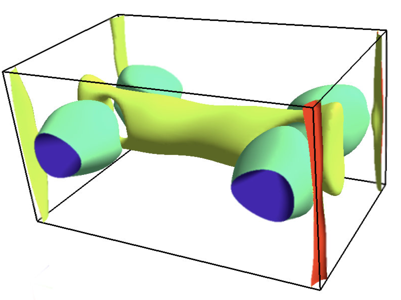
Figure 1: Fermi surface of FeP calculated on a ultra-dense k-grid in PAOFLOW and visualized in FermiSurfer [21]. For description of DFT calculations see Ref. [22].

3.16 gradient_and_momenta

The Hamiltonian’s gradient is initially calculated in real space, as it takes a simpler form. Afterward, it is Fourier transformed back into reciprocal space. Thus, the Hamiltonian’s k-space gradient is given by

$$\vec{\nabla}_{{\bf k}}\hat{H}({\bf k})=\sum_{\alpha}i{\bf R}\exp\left({i{\bf k}\cdot{\bf R}}\right)\hat{H}\left({\bf R}\right)$$ (3)

where $\hat{H}\left({\bf R}\right)$ is the real space PAO matrix and $\left|\psi_{n}({\bf k})\right>=\exp({-i{\bf k}\cdot{\bf r}})\left|u_{n}({\bf k})\right>$ are Bloch’s functions [23]. The Hamiltonian’s derivative is saved as a new array key ’dHksp’ in the DataController.

Next, the momenta are computed from the Hamiltonian’s gradient as

$${\bf p}_{nm}({\bf k}) = \left<\psi_{n}({\bf k})\right|\hat{p}\left|\psi_{m}({\bf k})\right>=$$

$$= \left<u_{n}({\bf k})\right|\frac{m_{0}}{\hbar}\vec{\nabla}_{\bf k}\hat{H}({\bf k})\left|u_{m}({\bf k})\right>$$

Additionally, the Hamiltonian’s second derivative can be computed by setting the band_curvature argument to True.

Arguments for gradient_and_momenta:

• band_curvature (bool) - Default: False - Compute the Hamiltonian’s second derivative, stored as an array in the DataController under the key ’d2Ed2k’.

3.17 adaptive_smearing

Generates the adaptive smearing parameters, stored in the DataController as ’deltakp’, used to compute quantities on energy intervals, such as the density of states or spin Hall conductivity. Allowed adaptive smearing types are gaussian (’gauss’), Methfessel-Paxton (’m-p’), or None. Implementation of the Gaussian broadening parameters are described in Section 3 of Ref [1].

Arguments for adaptive_smearing:

• smearing (string) - Default: ’gauss’ - Method of broadening used to smooth the discrete sampling of quantities computed on energy intervals.

3.18 dos

Compute the density of states (DOS) and/or projected density of states (PDOS) within a user defined energy range. If this routine is called after adaptive_smearing, the ’deltakp’ smearing parameter is used to smooth the DOS calculations.

Arguments for dos:

• do_dos (bool) - Default: True - Flag to control whether the DOS is computed.

• do_pdos (bool) - Default: True - Flag to control whether the PDOS is computed.

• delta (float) - Default: 0.01 - Width of the gaussian at each energy, used to smooth the dos curves. If it has been computed with the adaptive_smearing routine, ’deltakp’ replaces this quantity.

• emin (float) - Default: -10 - Lower limit for the energy range considered.

• emax (float) - Default: 2 - Upper limit for the energy range considered.

• ne (int) - Default: 1000 - The number of points to evaluate within the energy range [emin,emax].

3.19 z2_pack

Writes the real space Hamiltonian to a dat file, for use with the Z2Pack code [24].

Arguments for z2_pack:

• fname (string) - Default:
  ’z2pack_hamiltonian.dat’ - Name for the dat file, written to PAOFLOW’s output directory.

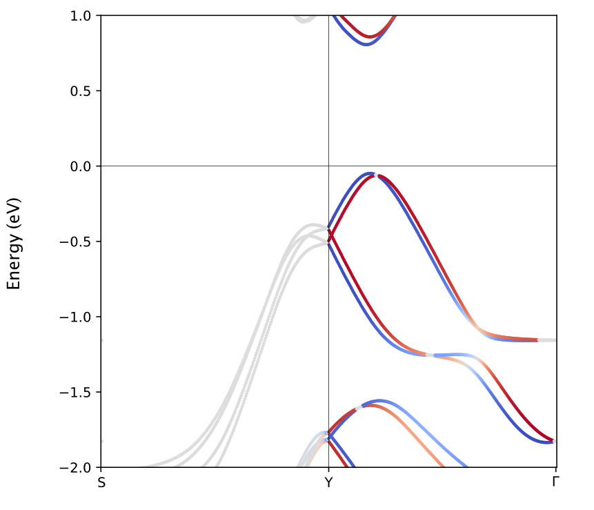
Figure 2: Spin texture ($S_{z}$) of two-dimensional ferroelectric SnTe along high-symmetry lines (example08). See Ref. [25]. for details.

3.20 spin_texture

Compute spin texture as the spin operator’s expectation value for each band and for each k-point:

$${\bf\Omega}_{n}({\bf k})=\langle\psi_{n}({\bf k})|{\bf S}_{j}|\psi_{n}({\bf k})\rangle$$ (5)

${\bf S}_{j}$ is the spin operator, and $|\psi_{n}({\bf k})\rangle$ are the momentum space PAO wavefunctions for band index $n$. The spin texture is computed for bands which have values within energy range specified by fermi_up and fermi_dw. Calling this routine after bands results in the spin texture along the same k-path as bands, while calling it after pao_eigh computes spin texture across the entire BZ. Results are written to a file named spin-texture-bands.dat for bands along a path and to NumPy .npz format with naming convention spin_text_band_N.npz for bands across the BZ. Here, N is the band index, and each file contains spin texture computed on PAOFLOW’s k-grid.

Arguments for spin_texture:

• fermi_up (float) - Default: 1 -The spin texture is computed only for bands which contain energies beneath this upper bound.

• fermi_dw (float) - Default: 1 - The spin texture is computed only for bands which contain energies above this lower bound.

3.21 anomalous_Hall

Calculating anomalous Hall conductivity (AHC, $\sigma_{ij}$) relies on accurate evaluation of the Berry curvature and requires a preliminary run of gradient_and_momenta. PAOFLOW implements a standard Kubo formula for evaluating the k-resolved Berry curvature [26]. Details are given in the previous paper and in the comprehensive reference by Gradhand et al. [27]. The AHC is computed with adaptive smearing, provided that the broadening parameters are calculated beforehand by adaptive_smearing.

Arguments for anomalous_Hall:

• do_ac (bool) - Default: False - Compute the magnetic circular dichroism (MCD) on the energy range [emin, emax].

• emin (float) - Default: -1 - The minimum energy in the range on which the AHC is computed.

• emax (float) - Default: 1 - The maximum energy in the range. 500 points are evaluated within the interval [emin, emax].

• fermi_up (float) - Default: 1 - Selects the upper energy bound for evaluating the Berry curvature.

• fermi_dw (float) - Default: -1 - Selects the lower energy bound for evaluating the Berry curvature.

• a_tensor (list) - Default: None - List of tensor elements to evalutate. For example, setting this argument to [[0,0], [1,2]] calculates the two components $\sigma_{xx}$ and $\sigma_{yz}$. All 9 components are computed, if the argument is left as None.

3.22 spin_Hall

The spin Hall conductivity (SHC, $\sigma^{k}_{ij}$) for spin polarization along k and charge (spin) current along i (j), is computed in a similar manner to AHC [28]. Here, evaluation of the spin Berry curvature is performed with the spin operator and Hamiltonian gradient as ingredients. Again, the gradient_and_momenta routine is a prerequisite, and running adaptive_smearing beforehand controls the inclusion of broadening parameters in the calculation.

Arguments for spin_Hall:

• twoD (bool) - Default: False - Setting this flag True outputs the spin_Hall quantities in 2-dimensional units $\Omega^{-1}$, removing any dependence on the sample height. It is assumed that the dimensions of interest are oriented in the x-y plane, and the slab is oriented along z.

• do_ac (bool) - Default: False - Compute the spin circular dichroism (SCD) on the energy range [emin, emax].

• emin (float) - Default: -1 - The minimum energy in the range on which the SHC and SCD are computed.

• emax (float) - Default: 1 - The maximum energy in the range. Again, 500 points are evaluated in the interval [emin, emax].

• fermi_up (float) - Default: 1 - Selects the upper energy bound for evaluating the spin Berry curvature.

• fermi_dw (float) - Default: -1 - Selects the lower energy bound for evaluating the spin Berry curvature.

• s_tensor (list) - Default: None - List of tensor elements to evalutate. To calculate $\sigma^{x}_{xx}$ and $\sigma^{z}_{xy}$ components use [[0,0,0],[0,1,2]]. If the argument is left as None, all 27 components are computed.

3.23 doping

Determine the chemical potential corresponding to a specified doping concentration and temperature range.

Arguments for doping:

• tmin (float) - Default: 300 - Minimum temperature for which to evaluate the chemical potential.

• tmax (float) - Default: 300 - Maximum temperature to compute chemical potential.

• nt (int) - Default: 1 - The number of temperatures to evaluate in the range [tmin, tmax].

• delta (float) - Default: 0.01 - Gaussian broadening width, used to smooth the density of states along the energy range. Doping calculation involves an integration over density of states and therefore includes a call to the dos module.

• emin (float) - Default: -1 - Lowest value of energy of the occupied bands.

• emax (float) - Default: 1 - At least the energy of the minimum of the conduction bands to obtain accurate results.

• ne (int) - Default: 1000 - Number of points in the energy grid.

• doping_conc (float) - Default: 0 - The doping concentration in carriers/cm³ for which to compute the chemical potential. Specify negative value for n-type doping and positive value for p-type doping.

• core_electrons (int) - Default: 0 - If the total number of electrons in the lower energy bands is known, this value can be introduced here. In this case, emin does not have to be the lowest energy value of occupied bands but can instead be set above energies of the core bands, to speed up integration.

• fname (string) - Default: ’doping_’ - Prefix for the output file containing doping versus temperature.

3.24 density

Calculate the electronic density on a real space grid, performed for silicon in Listing 4 and displayed in Figure 3. Wavefunctions in k-space (produced by pao_eigh) are required as a prerequisite, and the PAO projections must be performed by PAOFLOW’s projections method. This algorithm serves as a recipe for constructing the real space PAO wavefunctions. Although this is currently the only routine to utilize such construction, future versions of PAOFLOW will include other methods for computing spatially resolved quantities. The real space grid dimension defaults to 48x48x48 but can be specified with the optional arguments nr1, nr2, and nr3.

Arguments for density:

• nr1 (int) - Default: 48 - Number of points in the first dimension of the real space grid, over which to compute the charge density.

• nr2 (int) - Default: 48 - Number of points in the second dimension of the real space grid.

• nr3 (int) - Default: 48 - Number of points in the third dimension of the real space grid.

Figure 3: Electronic density for diamond structure of silicon on the $\langle 1,0,-1\rangle$ plane cut, calculated from the real space PAO wavefunctions (example01).

3.25 transport

Calculate the transport properties, such as electrical conductivity, Seebeck coefficients, and thermal conductivity. The transport properties are computed in the constant relaxation time approximation, unless built-in or user defined $\tau$ models are provided. See example09 for detailed information on specifying models for the relaxation time $\tau$.

Arguments for transport:

• tmin (float) - Default: 300 - Minimum temperature for which to evaluate transport properties.

• tmax (float) - Default: 300 - Maximum temperature to evaluate transport properties.

• nt (float) - Default: 1 - The number of temperatures to evaluate in the range [tmin,tmax].

• emin (float) - Default: 1 - Minimum value in the energy grid [emin,emax].

• emax (float) - Default: 10 - Maximum value of energy in the grid.

• ne (int) - Default: 1000 - Number of points in the energy range [emin,emax].

• scattering_channels (list) - Default: None - List of strings and/or TauModel objects containing the scattering models to be included in the calculation of $\tau$ .

• scattering_weights (list) - Default: None - Initial guess for the parameters $a_{imp}$, $a_{ac}$, $a_{op}$ etc to be used for the fitting procedure if fit is set to True. The default behavior with this argument set to None is to use unity as every scattering weight.

• tau_dict (dict) - Default: {} - Dictionary of parameters required for the calculation of scattering models.

• write_to_file (bool) - Default: True - Controls the output of the several data fields produced by this routine. No files are written if the flag is set to False.

• save_tensors (bool) - Default: False - Setting this flag True stores the resulting electrical conductivity, Seebeck coefficient, and thermal conductivity to the data_arrays dictionary with respective keys ’sigma’, ’S’, and ’kappa’.

3.26 find_weyl_points

Perform a search for Weyl points within the first Brillouin zone. The search identifies Weyl point candidates by utilizing Scipy’s minimize function with the ’L-BFGS-B’ algorithm.

Arguments for find_weyl_points:

• symmetrize (bool) - Default: False - Use QE symmetry operations to unfold equivalent k-points. If equivalent k-points are Weyl points, all such points are reported.

• search_grid (list) - Default: [8, 8, 8] - Dimensions of the grid on which the minimization routine is performed. Bands are Fourier interpolated on this grid to improve resolution.

3.27 restart_dump

PAOFLOW’s computational state can be saved at any time with the restart_dump routine. Data is stored in the json format, and the naming convention for such files can be chosen with the fname_prefix argument. Each processor saves a file in the workpath directory with name fname_prefix_N.json, where N is the core’s rank. For this reason, restarted calculations must be executed with the same number of cores. See Listing 5 for an example where the gradient and momenta are computed and dumped for reuse in another calculation.

Arguments for restart_dump:

• fname_prefix (string) - Default: ’paoflow_dump’ - The name prefix for the dump files, written to the working directory.

3.28 restart_load

Recover PAOFLOW’s calculation state from a previous run, saved to the json format with restart_dump. A restarted run must be executed with the same number of cores as the run which produced the dump files. Listing 6 provides example usage for restart_load.

Arguments for restart_load:

• fname_prefix (string) - Default: ’paoflow_dump’ - The name prefix for the dump files, written to the working directory.

3.29 finish_execution

Conclude the PAOFLOW run and remove references to memory intensive quantities. Details about the execution are provided, such as run duration and total memory requirements. This routine should be called once all desired calculations are performed for a given PAOFLOW object, especially if the code continues to create other PAOFLOW Hamiltonians.

finish_execution accepts no arguments.

4 Tight-binding models

PAOFLOW is capable of generating a Hamiltonian from analytical TB models, such as the Kane-Mele or Slater-Koster models [30, 29]. For each type of model, one needs to specify a few system properties, such as hopping parameters, lattice constant, etc. These parameters, including the label selecting the model to implement, should be initially stored in a dictionary, which is subsequently passed into PAOFLOW’s constructor as the model argument. Once the Hamiltonian is constructed, PAOFLOW’s class methods can be applied in the standard way to compute any desired quantities. Two examples are provided in Listing 7 and 8, and more are provided in the examples/ directory.

4.1 Cubium

Creates a Hamiltonian for a single atom in the simple-cubic geometry, containing one orbital per site. The hopping parameter is defined by including an entry in the parameters dictionary with key ’t’, and should have units of eV.

Required dictionary entries:

• Key: ’label’ - Keyword identifier for the model: ’cubium’, in this case. The labels are not case sensitive.

• Key: ’t’ - The hopping parameter for nearest neighbor interactions, in units of eV.

4.2 Cubium II

Creates a Hamiltonian for a single atom in the simple-cubic geometry, implementing the double band model with two orbitals per site. The hopping parameter and band gap energy are given by ’t’ and ’Eg’ respectively.
Required dictionary entries:

• Key: ’label’ - Keyword identifier for the model: ’cubium2’

• Key: ’t’ - The hopping parameter for nearest neighbor interactions.

• Key: ’Eg’ - Band gap energy, in eV.

4.3 Graphene

A simple TB model for graphene, considering only nearest neighbor interactions. The hopping parameter is specified with parameter ’t’. The lattice constant is taken as $a=2.46$ Å, and lattice vectors are given in a standard form: ${\bf a_{1}}=a\langle 1,0,0\rangle$, ${\bf a_{2}}=a\langle\frac{1}{2},\frac{\sqrt{3}}{2},0\rangle$, ${\bf a_{3}}=a\langle 0,0,10\rangle$.

Required dictionary entries:

• Key: ’label’ - Keyword identifier for the model: ’graphene’

• Key: ’t’ - The hopping parameter for nearest neighbor interactions.

4.4 Kane-Mele model

Constructs a Kane-Mele Hamiltonian for graphene. The first nearest neighbors are handled in the standard manner, with hopping parameter ’t’. Second nearest neighbors are treated with spin dependent amplitude, characterized by the parameter ’soc_par’. See an example in Listing 7.

Required dictionary entries:

• Key: ’label’ - Keyword identifier for the model: ’kane_mele’.

• Key: ’alat’ - The lattice parameter, $a$. The lattice vectors are the same as in section 4.3.

• Key: ’t’ - The hopping parameter for nearest neighbor interactions.

• Key: ’soc_par’ - The spin-orbit coupling parameter for second nearest neighbor interactions.

4.5 Slater-Koster model

A generalized Slater-Koster TB model in the two-center approximation, that includes only s and p orbitals of first nearest neighbors. The user must specify the lattice vectors, the atomic positions, the included orbitals for each atom, and the hopping parameters. See Listing 8 for further details.

Required dictionary entries:

• Key: ’label’ - Keyword identifier for the model: ’slater_koster’.

• Key: ’a_vectors’ - A numpy array containing the three primitive lattice vectors.

• Key: ’atoms’ - A dictionary with entries specifying atomic information for each atom. Dictionary keys label the atoms numerically with strings (e.g. the first atom has key ’0’), and the corresponding values are dictionaries with information about the atom. The species, position (in crystal coordinates), and string identifier for each represented orbital should be saved in the atomic dictionary with respective keys: ’name’, ’tau’, and ’orbitals’. The name is simply a string, the atomic position is a 3-vector, and orbitals are a list of strings denoting the orbitals belonging to each atom.

• Key: ’hoppings’ - A dictionary defining different hopping parameters, in eV. The Slater-Koster hopping parameters should be labeled: sss, sps, pps, and ppp.

5 Scattering models

PAOFLOW supports a diverse set of scattering effects by allowing users to implement temperature and energy dependent models for the relaxation time parameter $\tau$. Functional models are defined with the TauModel class. There are many built-in models, which only require the specification of empirical constants, and users can define new models to pass into PAOFLOW directly. A Python dictionary containing required parameters for any selected built-in models must be passed to the transport routine as the tau_dict argument (see Listing 9). Table 1 details the various constant parameters and their key strings for dictionary entries. Models for $\tau$ models are necessarily dependent on two quantities, the temperature and the Hamiltonian’s energy eigenvalues. Other varying parameters can be supplied to TauModels through the params dictionary. As such, a python function accepting three arguments (the temperature, the energy, and the parameters dictionary) is the required format when constructing a custom TauModel object. The $\tau$ for each included model are computed, by evaluating the TauModel functions. Then, the $\tau$s are harmonically summed to obtain the effective $\tau$ for all scattering channels. The functional form for a TauModel is presented in Listing 8 and a usage case in example10.

5.1 Charged impurity scattering

In order to include the effect of electron scattering from impurities, include ’impurity’ in the list scattering_channels [32, 31]. This calculates the relaxation time as

$$\tau_{im}(E,T)=\frac{E^{\frac{3}{2}}\sqrt{2m^{*}}4\pi\varepsilon^{2}}{(log(1+\frac{1}{x})-\frac{1}{1+x})\pi n_{I}Z_{I}^{2}e^{4}}\\$$ (6)

$$x=\frac{E}{k_{B}T}\\$$ (7)

Required parameters are $m^{*}$, $\varepsilon_{0}$, $\varepsilon_{\inf}$, $n_{I}$, $Z_{I}$.

5.2 Acoustic scattering

In order to include the effect of electron scattering from acoustic phonons, include ’acoustic’ in the list scattering_channels. This calculates the relaxation time according to [32, 31]

$$\tau_{ac}(E,T)=\frac{2\pi\hbar^{4}\rho v^{2}}{(2m^{*})^{\frac{3}{2}}k_{B}TD_{ac}^{2}\sqrt{E}}\\$$ (8)

Required parameters are $m^{*},\rho,v,D_{ac}$.

5.3 Optical scattering

In order to include the effect of electron scattering from optical phonons, include ’optical’ in the list scattering_channels. This calculates the relaxation time following [32, 31]

$$\tau_{op}(E,T)=\frac{\sqrt{2k_{B}T}\pi x_{o}\hbar^{2}\rho}{{m^{*}}^{\frac{3}{2}}{D_{op}}^{2}N_{op}\sqrt{x+x_{o}}+(N_{op}+1)\sqrt{x-x_{o}}}\\$$ (9)

$$N_{op}=\frac{1}{\exp\frac{{\hbar\omega_{l}}}{k_{B}{T}}-1},\\ x=\frac{E}{k_{B}T},\\ x_{o}=\frac{\hbar\omega_{l}}{k_{B}T},\\$$ (10)

Required parameters are $m^{*},\rho,\omega_{l},D_{op},N_{op}$.

5.4 Polar acoustic scattering

In order to include the effect of electron scattering from acoustic phonons in polar materials, include ’polar_acoustic’ in the list scattering_channels. This calculates the relaxation time following [32, 31]

$$\begin{split}\tau_{pac}(E,T)=\frac{\sqrt{2E}2\pi\varepsilon^{2}\hbar^{2}\rho v^{2}}{p^{2}e^{2}\sqrt{m^{*}}k_{B}T}\\ \times\left[1-\frac{\epsilon_{o}}{2E}\log(1+4\frac{E}{\epsilon_{o}})+\frac{1}{1+4\frac{E}{\epsilon_{o}}}\right]\end{split}$$ (11)

Required parameters are $m^{*},\varepsilon_{0},\varepsilon_{\inf},\rho,v,p$.

5.5 Polar optical scattering

In order to include the effect of electron scattering from optical phonons in polar materials, include ’polar_optical’ in the list scattering_channels. This calculates the relaxation time based on [32, 31, 33].

$$\begin{split}\tau_{pop}(E,T)=\\ \sum_{i}\frac{Z(E,T,\omega_{i}^{l})E^{\frac{3}{2}}}{C(E,T,\omega_{i}^{l})-A(E,T,\omega_{i}^{l})-B(E,T,\omega_{i}^{l})}\end{split}$$ (12)

$$A(E,T,\omega_{l})=n(\omega_{l}+1)\frac{f_{0}(E+\hbar\omega_{l})}{f_{0}(E)}[(2E+\hbar\omega_{l})$$ (13)

$$sinh^{-1}(\frac{E}{\hbar\omega_{l}})^{\frac{1}{2}}-[E(E+\hbar\omega_{l})]^{\frac{1}{2}}]$$

$$B(E,T,\omega_{l})=\theta(E-\hbar\omega_{l})n(\omega_{l})\frac{f_{0}(E-\hbar\omega_{l})}{f_{0}(E)}$$ (14)

$$[(2E-\hbar\omega_{l})cosh^{-1}(\frac{E}{\hbar\omega_{l}})^{\frac{1}{2}}$$

$$-[E(E-\hbar\omega_{l})]^{\frac{1}{2}}]$$

$$C(E,T,\omega_{l})=2E[n(\omega_{l}+1)\frac{f_{0}(E+\hbar\omega_{l})}{f_{0}(E)}$$ (15)

$$sinh^{-1}(\frac{E}{\hbar\omega_{l}})^{\frac{1}{2}}+\theta(E-\hbar\omega_{l})n(\omega_{l})$$

$$\frac{f_{0}(E-\hbar\omega_{l})}{f_{0}(E)}cosh^{-1}(\frac{E}{\hbar\omega_{l}})^{\frac{1}{2}}]$$

$$Z(\omega_{l})=\frac{2}{W_{0}(\hbar\omega_{l})^{\frac{1}{2}}},\,W_{0}(\omega_{l})=\frac{e^{2}\sqrt{2m^{*}\omega_{l}}\varepsilon^{-1}}{4\pi\hbar^{\frac{3}{2}}}$$ (16)

Required parameters are $m^{*},\varepsilon_{0},\varepsilon_{\inf},\omega_{LO}$.

Parameter	Symbol	Units	Key
Mass density	$\rho$	$kg/m^{3}$	$rho$
Low freq. dielectric constant	$\epsilon_{0}$	-	eps_0
High freq. dielectric constant	$\epsilon_{\infty}$	-	eps_inf
Acoustic velocity	$v$	m/s	v
Effective mass ratio	$m^{*}$	-	ms
Acoustic deformation potential	$D_{ac}$	eV	D_ac
Optical deformation potential	$D_{op}$	eV	D_op
Optical phonon energy	$\hbar\omega_{l}$	eV	hwlo
Number of impurities	$n_{I}$	$cm^{-3}$	nI
Charge on impurity	$Z_{I}$	-	Zi
Piezoelectric constant	$p$	$C/m^{2}$	piezo

Table 1: Symbols, units, and corresponding key in tau_dict for the parameters required in various scattering models.

5.6 Effective scattering time

$$\frac{1}{\tau_{total}(E,T)}=\frac{1}{\tau_{im}(E,T)}+\frac{1}{\tau_{ac}(E,T)}+...$$ (17)

The total scattering time is calculated as a harmonic sum of the specified scattering mechanisms, evaluated for each energy and temperature, Eq 17. The effective scattering time $\tau_{total}$ is computed for each energy and temperature during the execution of the transport routine.

6 Performance

Benchmark performance tests reveal excellent scaling for massively parallelized calculations. PAOFLOW exploits parallelization over bands whenever possible, primarily in the calculation of gradients. However, most routines are parallelized across the k-point mesh or path. PAOFLOW also possesses excellent scaling of memory requirements, in parallel runs. Increasing the number of processors can reduce the memory load on each processor, as many of the large arrays are distributed evenly among the cores. Performance is analyzed on a Dell PowerEdge R730 server with two 2.4GHz Intel Xeon E5-2680 v4 fourteen-core processors, and results for several examples are presented in Fig 4 and Fig 5. PAOFLOW demonstrates excellent scaling properties on manycore systems and possesses massively parallel capabilities.

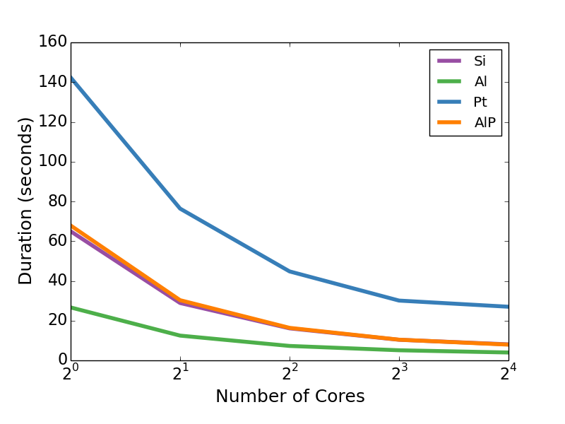
Figure 4: Selected examples (see examples/ on GitHub) performed on an increasing number of processors. Parallelized routines provide run time scaling nearly proportional to the number of cores used in a calculation, closely approaching the speed increase limit of Amdahl’s Law.

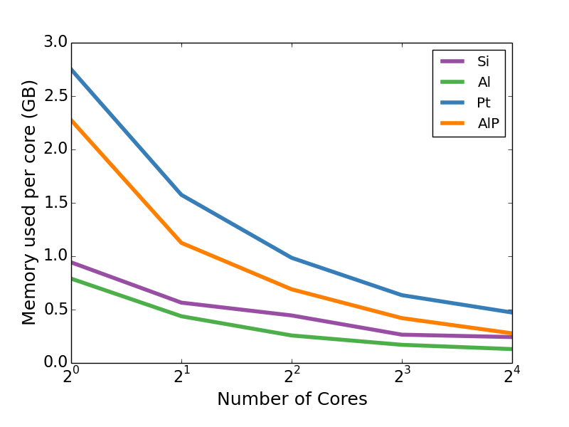
Figure 5: Memory scaling per core (in GB), for selected examples. An increasing core count reduces the memory requirements per processor.

7 Conclusions

PAOFLOW provides a lightweight, robust tool for efficient materials and Hamiltonian analysis. Continuous development of the package has streamlined its functionality and enabled many new tools for effectively characterizing the electronic properties of solids. The updated framework offers an ideal tool for high throughput condensed matter simulations and generation for materials genomics [34].

8 Acknowledgments

We are grateful for computational resources provided by the High Performance Computing Center at the University of North Texas and the Texas Advanced Computing Center at the University of Texas, Austin. The members of the AFLOW Consortium (http://www.aflow.org) acknowledge support by DOD-ONR (N00014-13-1-0635, N00014-11-1-0136, N00014-15-1-2863). The authors also acknowledge Duke University Center for Materials Genomics.

9 Data Availability

Data generated for this manuscript’s production is available on GitHub (https://github.com/marcobn/PAOFLOW), provided within the various examples directories outlined in the text above.

References

[1]
M. Buongiorno Nardelli, F. Cerasoli, M. Costa, S. Curtarolo, R. Gennaro, M. Fornari, L. Liyanage, A. Supka, and H. Wang, PAOFLOW: A utility to construct and operate on ab initio Hamiltonians from the Projections of electronic wavefunctions on Atomic Orbital bases (PAO), including characterization of topological materials, Computational Materials Science, 143, 462–472 (2018).
[2]
L. A. Agapito, S. Ismail-Beigi, S. Curtarolo, M. Fornari, and
M. Buongiorno Nardelli, Accurate tight-binding Hamiltonian matrices
from ab initio calculations: Minimal basis sets, Physical Review B
93, 035104–9 (2016).
[3]
L. A. Agapito, M. Fornari, D. Ceresoli, A. Ferretti, S. Curtarolo, and
M. Buongiorno Nardelli, Accurate tight-binding Hamiltonians for
two-dimensional and layered materials, Physical Review B 93,
125137–8 (2016).
[4]
Vu Thi Ngoc Huyen, Yuki Yanagi, and Michi-To Suzuki, Spin and anomalous Hall effects emerging from topological degeneracy in Dirac fermion system CuMnAs, Phys. Rev. B (2021).
[5]
Shao, Ding-Fu and Gurung, Gautam and Zhang, Shu-Hui and Tsymbal, Evgeny Y., Dirac Nodal Line Metal for Topological Antiferromagnetic Spintronics, Physical Review Latters 122, 077203 (2019).
[6]
T. Nan, C.X. Quintela, J. Irwin, G. Gurung, D.F. Shao, J. Gibbons, N. Campbell, K. Song, S.-Y. Choi, L. Guo, R.D. Johnson, P. Manuel, R.V. Chopdekar, I. Hallsteinsen, T. Tybell, P.J. Ryan, J.-W. Kim, Y. Choi, P.G. Radaelli, D.C. Ralph, E.Y. Tsymbal, M.S. Rzchowski, and C.B. Eom, Controlling spin current polarization through non-collinear antiferromagnetism, Nature Communications 2041-1723, 4671 (2020).
[7]
McHugh, Oliver L. W. and Goh, Wen Fong and Gradhand, Martin and Stewart, Derek A., Impact of impurities on the spin Hall conductivity in -W, Phys. Rev. Materials 4, 094404 (2020).
[8]
Gurung, Gautam and Shao, Ding-Fu and Paudel, Tula R. and Tsymbal, Evgeny Y., Anomalous Hall conductivity of noncollinear magnetic antiperovskites, Phys. Rev. Materials 3, 04409 (2019).
[9]
T. Hagiwara, K. Suekuni, P. Lemoine, A.R. Supka, R. Chetty, E. Guilmeau, B. Raveau, M. Fornari, M. Ohta, R. Al Rahal Al Orabi, H. Saito, K. Hashikuni, and M. Ohtaki
Key Role of d0 and d10 Cations for the Design of Semiconducting Colusites: Large Thermoelectric ZT in Compounds, Chemistry of Materials 33, 3449–3456 (2021).
[10]
V. Pavan Kumar, P. Lemoine, V. Carnevali, G. Guélou, O.I. Lebedev, P. Boullay, B. Raveau, R. Al Rahal Al Orabi, M. Fornari, C. Prestipino, D. Menut, C. Candolfi, B. Malaman, J. Juraszek, E. Guilmeau,
Ordered sphalerite derivative : a degenerate semiconductor with high carrier mobility in the Cu–Sn–S diagram, J. Mater. Chem. A 9, 10812–10826 (2021).
[11]
A. R. Supka, T. E. Lyons, L. Liyanage, P. D’Amico, R. Al Rahal Al Orabi,
S. Mahatara, P. Gopal, C. Toher, D. Ceresoli, A. Calzolari, S. Curtarolo,
M. Buongiorno Nardelli, and M. Fornari, AFLOW: A minimalist
approach to high-throughput ab initio calculations including the generation
of tight-binding hamiltonians, Computational Materials Science
136, 76–84 (2017).
[12]
S. Curtarolo, W. Setyawan, G. L. W. Hart, M. Jahnatek, R. V. Chepulskii, R. H.
Taylor, S. Wang, J. Xue, K. Yang, O. Levy, M. J. Mehl, H. T. Stokes, D. O.
Demchenko, and D. Morgan, AFLOW: An automatic framework for
high-throughput materials discovery, Computational Materials Science
58, 218–226 (2012).
[13]
S. Curtarolo, W. Setyawan, S. Wang, J. Xue, K. Yang, R. H. Taylor, L. J.
Nelson, G. L. W. Hart, S. Sanvito, M. Buongiorno Nardelli, N. Mingo, and
O. Levy, AFLOWLIB.ORG: A distributed materials properties repository
from high-throughput ab initio calculations, Comput. Mater. Sci.
58, 227–235 (2012).
[14]
P. Giannozzi, O. Andreussi, T. Brumme, O. Bunau, M. Buongiorno Nardelli, M. Calandra, R. Car, C. Cavazzoni, D. Ceresoli,
M. Cococcioni, N. Colonna, I. Carnimeo, A. Dal Corso, S. De Gironcoli, P. Delugas, R.A. DiStasio Jr, A. Ferretti,
A. Floris, G. Fratesi, G. Fugallo, R. Gebauer, U. Gerstmann, F. Giustino, T. Gorni, J. Jia, M. Kawamura, H.-Y. Ko,
A. Kokalj, E. Kucukbenli, M. Lazzeri, M. Marsili, N. Marzari, F. Mauri, N.L. Nguyen, H.-V. Nguyen, A. Otero-de-la-Roza,
L. Paulatto, S. Poncé, D. Rocca, R. Sabatini, B. Santra, M. Schlipf, A.P. Seitsonen, A. Smogunov, I. Timrov,
T. Thonhauser, P. Umari, N. Vast, X. Wu, and S. Baroni, Advanced capabilities for materials modelling with
Quantum ESPRESSO, Journal of Physics: Condensed Matter 29, 465901 (2017).
[15]
L. A. Agapito, S. Curtarolo, and M. Buongiorno Nardelli, Reformulation of DFT+U as a Pseudo-hybrid Hubbard Density Functional for Accelerated Materials Discovery, Physical Review X 5, 011006 (2015).
[16]
P. Gopal, M. Fornari, S. Curtarolo, L. A. Agapito, L. S. I. Liyanage, and
M. Buongiorno Nardelli, Improved predictions of the physical
properties of Zn- and Cd-based wide band-gap semiconductors: A validation of
the ACBN0 functional, Physical Review B 91, 245202 (2015).
[17]
L. A. Agapito, A. Ferretti, A. Calzolari, S. Curtarolo, and M. Buongiorno Nardelli, Effective and accurate representation of extended Bloch states on finite Hilbert spaces, Phys. Rev. B 88,
165127 (2013).
[18]
L. A. Agapito, S. Curtarolo, and M. Buongiorno Nardelli, Reformulation of as a Pseudohybrid Hubbard Density Functional for Accelerated Materials Discovery, Phys. Rev. X 5, 011006 (2015).
[19]
C. Toher, C. Oses, D. Hicks, E. Gossett, F. Rose, P. Nath, D. Usanmaz, D. C. Ford, E. Perim, E. E. Calderon, J. J. Plata, Y. Lederer, M. Jahnátek, W. Setyawan, S. Wang, J. Xue, K. Rasch, R. V. Chepulskii, R. H. Taylor, G. Gomez, H. Shi, A. R. Supka, R. Al Rahal Al Orabi, P. Gopal, F. T. Cerasoli, L. Liyanage, H. Wang, I. Siloi, L. A. Agapito, C. Nyshadham, G. L. W Hart, J. Carrete, F. Legrain, N. Mingo, E. Zurek, O. Isayev, A. Tropsha, S. Sanvito, R. M. Hanson, I. Takeuchi, M. J. Mehl, A. N. Kolmogorov, K. Yang, P. D’Amico, A. Calzolari, M. Costa, R. De Gennaro, M. Buongiorno Nardelli, M. Fornari, O. Levy, and S. Curtarolo,
The AFLOW Fleet for Materials Discovery, Springer, Cham (2017).
[20]
M. Graf and P. Vogl, Electromagnetic fields and dielectric response in empirical tight-binding theory, Physical Review B 51, 4940 (1995).
[22]
D. J. Campbell, J. Collini, J. Sławińska
and Autieri, C. Autieri, L. Wang, K. Wang, B. Wilfong, Y. S. Eo, P. Neves, D. Graf, E. E. Rodrigues, N. P. Butch, M. Buongiorno Nardelli, and J. Paglione, Topologically driven linear magnetoresistance in helimagnetic FeP, npj Quantum Materials 6, 38 (2021).
[23]
P. D’Amico, L. Agapito, A. Catellani, A. Ruini, S. Curtarolo, M. Fornari, M. Buongiorno Nardelli, and A. Calzolari, Accurate ab initio tight-binding Hamiltonians: Effective tools for electronic transport and optical spectroscopy from first principles, Phys. Rev. B 94, 165166 (2016).
[24]
D. Gresch, G. Autès, O. V. Yazyev, M. Troyer, D. Vanderbilt, B. A. Bernevig, A. A. Soluyanov,
Z2Pack: Numerical implementation of hybrid Wannier centers for identifying topological materials, Phys. Rev. B. 95, 075146 (2017).
[25]
J. Sławińska, F. T. Cerasoli, P. Gopal, M. Costa, S. Curtarolo, and M. Buongiorno Nardelli, Ultrathin SnTe films as a route towards all-in-one spintronics devices, 2D Materials 7, 025026 (2020).
[26]
Y. Yao, L. Kleinman, A. H. MacDonald, J. Sinova, T. Jungwirth, D.-s. Wang, E. Wang, and Q. Niu, First Principles Calculation of Anomalous Hall Conductivity in Ferromagnetic bcc Fe, Physical Review Lett 92, 037204–4 (2004).
[27]
M. Gradhand, D. V. Fedorov, F. Pientka, P. Zahn, I. Mertig, and B. L. Györffy, First-principle calculations of the Berry curvature of Bloch states for charge and spin transport of electrons, Journal of Physics: Condensed Matter 24, 213202–24 (2012).
[28]
G. Y. Guo, S. Murakami, T. W. Chen, and N. Nagaosa, Intrinsic Spin Hall Effect in Platinum: First-Principles Calculations, Physical Review Letters 100, 096401–4 (2008).
[29]
C. L. Kane and E. J. Mele, Quantum Spin Hall Effect in Graphene, Phys. Rev. Lett. 95, 226801 (2005).
[30]
J. C. Slater and G. F. Koster,
Simplified LCAO Method for the Periodic Potential Problem, Phys. Rev. 94, 1498–1524 (1954).
[31]
R. Farris, M. B. Maccioni, A. Filippetti, and V. Fiorentini, Theory of thermoelectricity in with an energy- and temperature-dependent relaxation time, Journal of Physics: Conference Series 1226, 012010 (2019).
[32]
C. Jacoboni, Theory of electron transport in semiconductors: a pathway from elementary physics to nonequilibrium Green functions, Journal of Physics: Cond. Matter 31, 065702 (2018).
[33]
B. Ridley, Polar-optical-phonon and electron-electron scattering in large-bandgap semiconductors, (Journal of Physics: Condensed Matter) 10, 6717 (1998).
[34]
W. Setyawan and S. Curtarolo, High-throughput electronic band structure calculations: Challenges and tools, Comput. Mater. Sci. 49,
299–312 (2010).