Free-free absorption in hot relativistic flows: application to fast radio bursts

Abstract

Magnetic flares create hot relativistic shocks outside the light cylinder radius of a magnetised star. Radio emission produced in such a shock or at a radius smaller than the shock undergoes free-free absorption while passing through the shocked medium. In this work, we demonstrate that this free-free absorption can lead to a negative drift in the frequency-time spectra. Whether it is related to the downward drift pattern observed in fast radio bursts (FRBs) is unclear. However, if the FRB down drifting is due to this mechanism then it will be pronounced in those shocks that have isotropic kinetic energies $\!\!\!\phantom{\geq}\smash{\buildrel\over{\lower 2.67502pt\hbox{$\buildrel\lower 2.14001pt\hbox{$\displaystyle>$}\over{\sim}$}}}\,\,10^{44}$ erg. In this model, for an internal shock with a Lorentz factor $\sim 100$, the normalised drift rate $|{\rm DR_{\rm obs}}|/\nu_{\rm mean}$ is $\sim 10^{-2}$ per ms, where $\nu_{\rm mean}$ is the central frequency of the radio pulses. The corresponding radius of the shocked shell is, therefore, in the range of $10^{10}$ cm and $10^{11}$ cm. This implies that, for an outflow consisting of hydrogen ion, the upper limit on the mass of the relativistic shocks is a few $\times~{}10^{-10}~{}\hbox{M${}_{\odot}$}$, which is considerably low compared to that ejected from SGR 1806-20 during the 2004 outburst.

1 Introduction

Astrophysical shocks are often considered to be associated with the most energetic events in the universe. After the death of massive stars, destruction of WDs, or mergers of compact objects, shocks are expected to be launched into the ambient medium (Chevalier, 1982; Matzner & McKee, 1999; Mészáros & Rees, 1997). For a normal core collapse supernova or thermonuclear runway explosions, these supernova-driven shocks are usually non-relativistic, expanding in the surrounding media with a speed $\sim$ a few $\times 10^{4}$  km s^-1(Chevalier & Fransson, 2017; Parrent et al., 2014). Some special supernovae and compact binary coalescence of two neutron stars (NSs) or a NS and black hole can launch relativistic outflows that power energetic gamma rays bursts (GRBs) (Mészáros, 2006; Zhang, 2018a). In the case of GRBs, both internal and external relativistic shocks are possible, with the former believed to power the observed $\gamma$-ray emission (Rees & Meszaros, 1994) and the latter believed to power the multi-wavelength afterglow (Mészáros & Rees, 1997; Sari et al., 1998). These shocks may produce low frequency radio bursts through synchrotron maser mechanisms (Usov & Katz, 2000; Sagiv & Waxman, 2002; Lyubarsky, 2014; Beloborodov, 2017; Waxman, 2017; Plotnikov & Sironi, 2019; Metzger et al., 2019; Beloborodov, 2020; Yu et al., 2021).

Fast radio bursts (FRBs) are mysterious radio transients from cosmological distances (Lorimer et al., 2007; Petroff et al., 2019; Cordes & Chatterjee, 2019). It is unclear what astrophysical objects are the main sources of FRBs and whether they are generated within the magnetosphere of a highly magnetized object (e.g. a magnetar) or from relativistic shocks (Zhang, 2020). The very high observed event rate, e.g. more than $10^{3}$ $\rm sky^{-1}$ events everyday (Petroff et al., 2019), suggests a high event rate density, i.e. $\sim 10^{4}$ $\rm Gpc^{-3}\rm yr^{-1}$ (Luo et al., 2020a; Ravi, 2019). One therefore is expected to detect a few of them from the nearby galaxies or even in Milky Way within a reasonable time interval. The discovery of the galactic FRB 200428 in association with the galactic magnetar SGR 1934+2154 (CHIME/FRB Collaboration et al., 2020; Bochenek et al., 2020; Mereghetti et al., 2020; Li et al., 2021; Ridnaia et al., 2021) confirmed this and suggested that at least magnetars can make FRBs.

The immediate surrounding of the FRB sources may cause the radio wave signal to undergo several absorption and scattering processes. For example, a radio wave may suffer from free-free absorption (Luan & Goldreich, 2014; Murase et al., 2016; Yang & Zhang, 2017; Kundu & Ferrario, 2020), induced Compton and Raman scattering (Lyubarsky, 2008; Lu & Kumar, 2018; Kumar & Lu, 2020; Ioka & Zhang, 2020), and synchrotron absorption (Yang et al., 2016) before making a way out of its production sites. Some of these conditions demand that the FRB outflow moves with a relativistic speed (e.g. Murase et al., 2016). In the following, we discuss what happens when a low frequency signal, produced by whatever physical mechanism, passes through a hot relativistic shell and undergoes free-free absorption in that medium. The applications and the consequences of this absorption process to FRBs are examined and discussed in $\S$ 3 and $\S$ 4.

2 Free-free absorption in a hot relativistic shell

We consider two shells with a relative Lorentz factor $\Gamma_{\rm rel}$ collide and drive a pair of internal shocks. If the two shells merge after the collision and have a bulk Lorentz factor $\Gamma$, the lab-frame total energy can be estimated as

$$E=N\Gamma(\Gamma_{\rm rel}-1)m_{p}c^{2},$$ (1)

where $m_{p}$ and $c$ are the proton mass and the velocity of light in vacuum, respectively, and $N=4\pi nr^{2}\Delta r$ is the total number of protons in the shell, $n$ is the number density of the protons in the lab-frame, We consider two relativistic shells with a not-too-large relative Lorentz factor, so that $r=c\Gamma^{2}t_{\rm obs}$ is the radius of the shock from the central engine, $\Delta r$ is the thickness of the shock in the lab-frame, and $t_{\rm obs}$ is the time in the observer frame. Combining these, we get

$$n=\frac{E}{4\pi m_{p}c^{4}t_{\rm obs}^{2}(\Delta r)\Gamma^{5}(\Gamma_{\rm rel}-1)},$$ (2)

The particle number density in the comoving frame, $n^{\prime}$, is related to the density in the lab frame, $n$, through $n=n^{\prime}\Gamma$. Similarly, $\Delta r=\Delta r^{\prime}/\Gamma$. The frequency in the observer frame, $\nu_{\rm obs}$, is approximately equal to $2\Gamma\nu^{\prime}$. Since the particles are relativistic in the shock comoving frame, in this frame the free-free absorption coefficient can be written as

$$\alpha_{\nu^{\prime}}^{\rm{}^{\prime}ff}=0.018Z^{2}\bar{g}^{\prime}_{\rm ff}T^{\prime-3/2}n^{\prime}_{e}n^{\prime}_{i}\nu^{\prime-2}(1+AT^{\prime})$$ (3)

(Rybicki & Lightman, 1979), with $A=4.4\times 10^{-10}$ K^-1. Here $Z$ is the atomic number of the gas. $n^{\prime}_{e}$ and $n^{\prime}_{i}$ represent the densities of electrons and ions in the shock, respectively. Again we assume that the shell is made up of hydrogen ion. Therefore, $n^{\prime}_{e}=n^{\prime}_{i}(\equiv n^{\prime})$ and $Z=1$. Also $\bar{g}^{\prime}_{\rm ff}$ represents the velocity averaged Gaunt factor and $T^{\prime}$ is the temperature of the electrons in the shock comoving frame. When the shocked energy is shared between electrons and protons, the temperature of the electrons behind the shock depends on the shock kinematics through the following relation

$$T^{\prime}=\frac{\epsilon_{e}(m_{p}/m_{e})}{k_{B}}(\Gamma_{\rm rel}-1)m_{e}c^{2},$$ (4)

(Meszaros & Rees, 1993), where $\epsilon_{e}$ is the fraction of the post shock energy that goes to electron. $k_{B}$ is the Boltzmann constant and $m_{e}$ represents electron mass. Assuming $\epsilon_{e}=0.1$, one gets $T^{\prime}\approx 1.1\times 10^{12}$ K for $(\Gamma_{\rm rel}-1)\approx 1$. Thus, $1+A~{}T^{\prime}\approx A~{}T^{\prime}$. Radio pulses remain trapped in this shock until the medium is optically thick to the waves. When it becomes transparent to a given frequency the optical depth for that frequency in the shock becomes unity, i.e.,

$$\alpha_{\nu^{\prime}}^{\rm{}^{\prime}ff}\Delta r^{\prime}=1,$$ (5)

which gives $t_{\rm obs}^{4}=AT^{\prime-1/2}~{}\nu_{\rm obs}^{-2}\eta_{1}$, with

$$\eta_{1}=0.018\frac{4}{c^{4}(\Delta r)\Gamma^{9}(\Gamma_{\rm rel}-1)^{2}}\bigg{(}\frac{E}{4\pi m_{p}c^{2}}\bigg{)}^{2}.$$ (6)

Therefore,

$$t_{\rm obs}=\frac{A^{1/4}T^{\prime-1/8}\eta}{\sqrt{\nu_{\rm obs}}},$$ (7)

where

$$\eta=\eta_{1}^{1/4}.$$ (8)

If $t_{{\rm obs},1}$ and $t_{{\rm obs},2}$ are the times when the shell becomes transparent to $\nu_{\rm obs,1}$ and $\nu_{\rm obs,2}$, then the drift rate, $\rm DR$, can be approximated as

$${\rm DR}=\frac{\nu_{\rm obs,2}-\nu_{\rm obs,1}}{t_{{\rm obs},2}-t_{{\rm obs},1}}.$$ (9)

This implies

$$\rm DR=-\frac{T^{\prime 1/8}}{A^{1/4}\eta}~{}\sqrt{\nu_{\rm obs,2}\nu_{\rm obs,1}}(\sqrt{\nu_{\rm obs,2}}+\sqrt{\nu_{\rm obs,1}}).$$ (10)

Note that the inverse scaling between $t_{\rm obs}$ and $\nu_{\rm,obs}$ in Eq.(7) stems from the $\propto\nu^{-2}$ in Eq.(3), which does not depend on whether the shock is relativistic, but a relativistic internal shock is needed to make the drift rate matching the observations. It is also needed to satisfy the duration and induced Compton scattering constraints if the shocks are the sites of FRBs. For the drift rate expressed in MHz/ms, and denoted as $\rm DR_{\rm obs}$, the above equation gives

$$\begin{split}\eta=-\frac{T^{\prime 1/8}}{A^{1/4}{\rm DR_{\rm obs}}}\sqrt{(\nu_{\rm obs,2})_{\rm MHz}(\nu_{\rm obs,1})_{\rm MHz}}~{}\\ \Bigg{[}\sqrt{(\nu_{\rm obs,2})_{\rm MHz}}+\sqrt{(\nu_{\rm obs,1})_{\rm MHz}}\Bigg{]},\end{split}$$ (11)

where $(\nu_{\rm obs})_{\rm MHz}$ represents frequency in MHz in the observer frame. Notice that when $\nu_{\rm obs,2}$ and $\nu_{\rm obs,1}$ are close to each other, their arithmetic mean would be similar to their geometric mean, so that $\eta$ is inversely proportional to the normalized drift rate ${\rm DR_{\rm obs}}/\nu_{\rm mean}$, as shown in Figure 1 (discussed below).

3 Application to Fast radio bursts

FRBs have been detected from 110 MHz (Pastor-Marazuela et al., 2020) to 8 GHz (Gajjar et al., 2018) with a minimum and maximum width of the pulses of around 30 $\mu$s (Michilli et al., 2018) and 26 ms (Farah et al., 2017) detected from FRB 121102 and FRB 170922, respectively. One interesting feature of FRBs, especially of those repeating ones, is the sub-pulse drifting of frequency. Low frequency subpulses are observed to be delayed with respect to high-frequency ones (Hessels et al., 2019; CHIME/FRB Collaboration et al., 2019a, b; Fonseca et al., 2020; Pastor-Marazuela et al., 2020; Luo et al., 2020b). The observed drift rates for CHIME FRBs are in the range 1 MHz/ms to 30 MHz/ms with one of the bursts from the second repeating FRB 180814.J0422+73 having a minimum drift rate of $\sim 1$ MHz/ms. At higher frequencies, the drift rates have increased significantly as exhibited by bursts from the first repeating FRB 121102, though some of the bursts of FRB 180916B, detected with the Apertif telescope, displays a drift rate as small as 4 MHz/ms in the L band.

We apply the free-free absorption theory discussed in Section 2 to FRBs and to investigate whether it can interpret the down-drifting feature. Since FRBs are millisecond duration transient radio pulses, one can take $\Delta t_{\rm obs}\sim 1$ ms. The millisecond duration of the bursts implies that the characteristic length scale of the emission region is $\Delta r\sim c\Delta t_{\rm obs}\sim 3\times 10^{7}$ cm. Inserting this value of $\Delta r$ in Eq. 6 and using Eq.8 we obtain

$$\Gamma^{9}(\Gamma_{\rm rel}-1)^{2}=\frac{8.3\times 10^{42}}{\eta^{4}}E_{\rm 45}^{2},$$ (12)

where $E_{\rm 45}=E(\rm erg)/10^{45}$ erg. Over the frequency range of 400 MHz to 7 GHz, the observed drift rates, $\rm DR_{\rm obs}$, of different bursts vary from $\sim-1$ MHz/ms to $-870$ MHz/ms. The emission bandwidth of most of the bursts is small: for the CHIME bursts it is around $200$ MHz. From Eq.8, the estimated values of $\eta$ for an internal shock are in the range of $2\times 10^{6}$ to $2\times 10^{8}$ ms MHz^1/2 K^-1/8, where $T^{\prime}=1.1\times 10^{12}$ K. Figure 1 displays the required $\eta$ as a function of $|{\rm DR_{\rm obs}}|/\nu_{\rm mean}$ with $\nu_{\rm mean}=(\nu_{\rm obs,2}+\nu_{\rm obs,1})/2$, which represents the central frequency of the observed radio pulse. The values of the DR of different FRBs were published in Hessels et al. (2019); CHIME/FRB Collaboration et al. (2019b); Fonseca et al. (2020); Pastor-Marazuela et al. (2020). The filled diamonds, triangles and circles represent the CHIME repeaters, FRB 121102 and FRB 180916B, respectively, where the second repeating FRB 180814.J0422+73 is included in the CHIME sample.

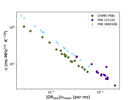
Figure 1: The required $\eta$ as a function of modulus of $\rm DR_{\rm obs}$ divided by the central frequency of the observed pulse for an internal shock. The $\rm DR_{\rm obs}$ of different FRBs are taken from Hessels et al. (2019); CHIME/FRB Collaboration et al. (2019b); Fonseca et al. (2020); Pastor-Marazuela et al. (2020). The filled diamonds, triangles and circles represent the CHIME repeaters, FRB 121102 and FRB 180916B, respectively. The CHIME sample includes the second repeating FRB 180814.J0422+73.

The magnetic energy stored in a magnetar with a radius $\sim$ 10 km and a characteristic magnetic field $B\sim 10^{15}$ G (Duncan & Thompson, 1992) is $\!\!\!\phantom{\geq}\smash{\buildrel\over{\lower 2.67502pt\hbox{$\buildrel\lower 2.14001pt\hbox{$\displaystyle>$}\over{\sim}$}}}\,\,10^{47}$ erg. For $B\!\!\!\phantom{\geq}\smash{\buildrel\over{\lower 2.67502pt\hbox{$\buildrel\lower 2.14001pt\hbox{$\displaystyle>$}\over{\sim}$}}}\,\,10^{16}$ G the dipolar magnetic energy could be as high as $10^{49}$ erg. The giant flare detected from SGR 1806-20 in 2004, during a hyperactive phase, had an isotropic flare energy of around $2\times 10^{46}$ erg (Palmer et al., 2005). Moreover, it was found that a similar amount of energy was released from a magneter in NGC 253 during an extremely bright gamma-ray burst event on 15th April 2020 (Svinkin et al., 2021). For $\eta$ in the range from $2\times 10^{6}$ to $2\times 10^{8}$ ms MHz^1/2 K^-1/8, the allowed values of $\Gamma$ (estimated using eq.12) as a function of the shock energy $E$ varying from $10^{44}$ erg to $10^{46}$ erg are shown in Fig.2. We note that free-free absorption is pronounced for shocks having higher kinetic energies, $\gtrsim 10^{44}$ erg (otherwise, $\Gamma$ is too small to satisfy the drift-rate constraint).

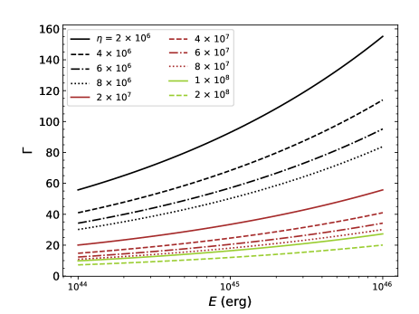
Figure 2: The allowed values of $\Gamma$ as a function of shock energy, $E$, for $\eta$ in the range $2\times 10^{6}$ to $2\times 10^{8}$ ms MHz^1/2 K^-1/8.

The particle density in the shocks is

$$n=\frac{2.4\times 10^{-25}\eta^{4}\Gamma^{4}(\Gamma_{\rm rel}-1)}{t_{\rm obs}^{2}E_{\rm 45}},$$ (13)

as obtained from Eqs.2 and 12. Assuming that shocks are solely made up of hydrogen and $t_{\rm obs}\sim 1$ ms, the mass of the shells, $M_{\rm sh}$, as a function of $E$ is depicted in Fig.3 for different values of $\eta$, estimated for an internal shock. For $E\sim 10^{44}$ erg, $M_{\rm sh}$ is around $10^{-12}$ M_⊙; and it is about two orders of magnitude higher when the shock energy is $10^{46}$ erg. For an active magnetar, the maximum mass of the ejected material during a flaring event could be $\sim 10^{-5}$ M_⊙(Beloborodov, 2017). In our model, even when the highest energy outbursts occur everyday, a magnetar would require around 100 yr to eject a total of $\sim 10^{-5}$ M_⊙matter in the surrounding medium.

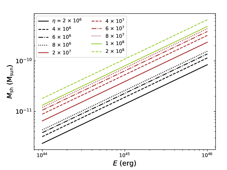
Figure 3: The mass of the shell, $M_{\rm sh}$, as a function of shock energy $E$ for different values of $\eta$ obtained for an internal shock.

The radius of the shell as a function of the shock energy $E$ for different values of $\eta$ is displayed in Fig.4. Since relativistic shocks are expected to form beyond the magnetosphere, we also draw the magnetar light cylinder (LC) radius $R_{\rm LC}\simeq cP/(2\pi)$ (which defines the outer boundary of the magnetosphere) for comparison, where $P$ is the magnetar spin period. In the figure, the cyan, red and blue horizontal lines exhibit the radii of the LC for $P=$ 1 s, 3 s and 10 s, respectively. Assuming that the spindown energy loss of a magnetar is dominated by magnetic dipole radiation, the characteristic age of the magnetar can be estimated as $\tau\simeq{P}/(2\dot{P})$, where the braking index of the magnetar is presumed to be 2, and $\dot{P}$ represents the derivative of the period. For a magnetar of mass $1.4~{}\hbox{M${}_{\odot}$}$ and radius 10 km, an upper limit on $\dot{P}$ is calculated as $\dot{P}({\rm{s\ s^{-1}}})=[B({\rm{G}})/(3\times 10^{19})]^{2}/{P(\rm{s})}$. Considering $B=10^{15}$ G, the age $\tau$ of the magnetar is found to be around 16 yr, 146 yr and 1622 yr for $P=$ 1 s, 3 s and 10 s, respectively. This implies that the older the population, the smaller the $\eta$ values for free-free absorption to be a relevant process to produce the observed down drifting in the frequency-time plane.

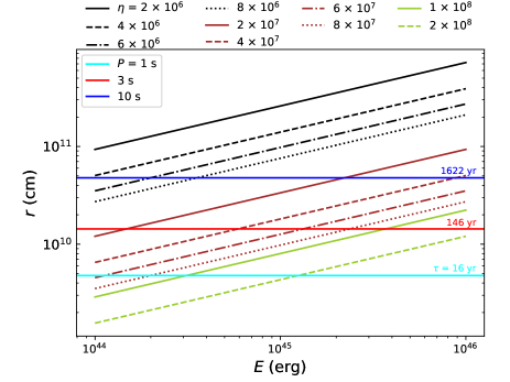
Figure 4: Radius of the shell as a function of shock energy $E$ for different values of $\eta$. The cyan, red and blue horizontal lines display the radius of the LC when the period $P$ of a magnetar is 1 s, 3 s and 10 s, respectively. The age of the magnetar corresponding to each $P$ is shown in the plot, assuming that the spindown energy loss is dominated by magnetic dipole radiation.

4 Discussion

FRBs from magnetars have been interpreted within the framework of two types of models. One group of models suggests that coherent emission originates from the magnetosphere of the neutron star (Kumar et al., 2017; Yang & Zhang, 2018, 2021; Lu & Kumar, 2018; Lu et al., 2020), while the other group of models interprets coherent emission as synchrotron maser in relativistic shocks (Lyubarsky, 2014; Beloborodov, 2017; Waxman, 2017; Plotnikov & Sironi, 2019; Metzger et al., 2019; Beloborodov, 2020). Within the magnetosphere model, the frequency down-drifting has been interpreted as a consequence of “radius-to-frequency mapping” commonly observed in radio pulsars, i.e. emission with different frequencies originate from different altitudes and the high-frequency emission is observed earlier than low-frequency one (Wang et al., 2019; Lyutikov, 2020). Within the synchrotron maser model, the drift is interpreted as due to emitting frequency decreasing with radius in relativistic shocks (Metzger et al., 2019; Beloborodov, 2020). Polarization angle swings of some FRBs favor the magnetosphere origin of FRBs (Luo et al., 2020b), but it is unclear whether the shock model may be responsible for some FRBs.

In this work, we illustrate that the free-free absorption in relativistic shocks introduces a feature of down-drifting. Whether it is related to the FRB phenomenology is unclear. However, if the FRB down drifting is due to this mechanism then the following conditions should be satisfied: i.) there should be a hot relativistic shell through which the radio waves pass through and ii.) the energy of this shock should be $\!\!\!\phantom{\geq}\smash{\buildrel\over{\lower 2.67502pt\hbox{$\buildrel\lower 2.14001pt\hbox{$\displaystyle>$}\over{\sim}$}}}\,\,10^{44}$ erg. In this model, the shell serves as the absorber of the radio waves. The radiation may originate from the shock, similar to what happens in the case of synchrotron maser model of FRBs, or could be produced at a radius smaller than the hot shell, e.g. from the magnetosphere of the central engine. These shocks are expected to have $\Gamma$ much greater than unity. In the case of an internal shock, this criteria is fulfilled except for $\eta\sim 10^{8}$ ms MHz^1/2 K^-1/8 and $E<10^{45}$ erg. The majority of the bursts (see Fig.1) require $\eta<4\times 10^{7}$ ms MHz^1/2 K^-1/8. For $\eta\sim 10^{6}$ ms MHz^1/2 K^-1/8 and $E\sim 10^{45}$ erg, $\Gamma$ is $\sim 100$ (see Fig.2). The smaller values of the $\eta$ imply larger shock radii (see Fig.4). For the shocks with a radius $\sim 10^{9}$ cm from the central engine, the magnetar that powers FRBs could be as young as a couple of decade old, as demonstrated in Fig.4 based on the assumption that the spin down energy loss is dominated by the magnetic dipole radiation. Furthermore, the mass of the shocked shell is less than a few $\times 10^{-10}$ M_⊙ as shown in Fig.3. This suggests that our model may work even for a magnetar that is active for $\!\!\!\phantom{\geq}\smash{\buildrel\over{\lower 2.67502pt\hbox{$\buildrel\lower 2.14001pt\hbox{$\displaystyle>$}\over{\sim}$}}}\,\,100$ yr and flares almost every day.

Particle-in-cell simulations of synchrotron maser emission from relativistic shocks suggests that the efficiency of this mechanism is $7\times 10^{-4}/\sigma^{2}$, for $\sigma\!\!\!\phantom{\geq}\smash{\buildrel\over{\lower 2.67502pt\hbox{$\buildrel\lower 2.14001pt\hbox{$\displaystyle>$}\over{\sim}$}}}\,\,1$, where $\sigma$ is the magnetisation parameter (Plotnikov & Sironi, 2019). This implies that the efficiency of synchrotron maser is very low requiring a large amount of energy to go to other wavelengths. The observed radio-to-X-ray flux ratio for FRB 200428 associated with the Galactic magneter SGR 1934+2154 (Mereghetti et al., 2020; Li et al., 2021; Ridnaia et al., 2021; Tavani et al., 2021; CHIME/FRB Collaboration et al., 2020; Bochenek et al., 2020) roughly satifies this constraint (Margalit et al., 2020), even though the magnetoshere model can also interpret this ratio (Lu et al., 2020; Yang & Zhang, 2021). The energy of the localised cosmological FRBs are in the range $10^{27}-10^{34}$ erg/Hz (Tendulkar et al., 2017; Bannister et al., 2019; Ravi et al., 2019; Marcote et al., 2020; Law et al., 2020; Bhandari et al., 2020a, b). Using the dispersion measure-redshift (Deng & Zhang, 2014) relation Zhang (2018b) demonstrates that the peak luminosities of the FRBs are in the range $10^{42}-10^{45}$ erg $\rm{s}^{-1}$. These imply that the radio energy of the cosmological FRBs vary between $10^{36}-10^{43}$ erg. Even though no simultaneous X-ray bursts has been detected from cosmological FRBs despite attempts (Scholz et al., 2016), if one assumes that the X-ray-to-radio luminosity ratio of these FRBs is similar to that of FRB 200428, one would expect that the total energy of these events is at least $10^{40}-10^{47}$ erg. For $E>10^{44}$ erg free-free absorption in shocks would be important in producing the downward drift in frequency-time as demonstrated in Fig.2. As a result, the mechanism discussed in this paper should be considered in FRB modeling and may be relevant to the down-drifting feature observed in at least some FRBs.

Data Availability

The data underlying this article will be shared on reasonable request to the corresponding author.

References

- Bannister et al. (2019) Bannister K. W., et al., 2019, Science, 365, 565
- Beloborodov (2017) Beloborodov A. M., 2017, ApJ, 843, L26
- Beloborodov (2020) Beloborodov A. M., 2020, ApJ, 896, 142
- Bhandari et al. (2020a) Bhandari S., et al., 2020a, ApJ, 895, L37
- Bhandari et al. (2020b) Bhandari S., et al., 2020b, ApJ, 901, L20
- Bochenek et al. (2020) Bochenek C. D., Ravi V., Belov K. V., Hallinan G., Kocz J., Kulkarni S. R., McKenna D. L., 2020, Nature, 587, 59
- CHIME/FRB Collaboration et al. (2019a) CHIME/FRB Collaboration et al., 2019a, Nature, 566, 235
- CHIME/FRB Collaboration et al. (2019b) CHIME/FRB Collaboration et al., 2019b, ApJ, 885, L24
- CHIME/FRB Collaboration et al. (2020) CHIME/FRB Collaboration et al., 2020, Nature, 587, 54
- Chevalier (1982) Chevalier R. A., 1982, ApJ, 258, 790
- Chevalier & Fransson (2017) Chevalier R. A., Fransson C., 2017, Thermal and Non-thermal Emission from Circumstellar Interaction. p. 875, doi:10.1007/978-3-319-21846-5_34
- Cordes & Chatterjee (2019) Cordes J. M., Chatterjee S., 2019, ARA&A, 57, 417
- Deng & Zhang (2014) Deng W., Zhang B., 2014, ApJ, 783, L35
- Duncan & Thompson (1992) Duncan R. C., Thompson C., 1992, ApJ, 392, L9
- Farah et al. (2017) Farah W., et al., 2017, The Astronomer’s Telegram, 10867, 1
- Fonseca et al. (2020) Fonseca E., et al., 2020, ApJ, 891, L6
- Gajjar et al. (2018) Gajjar V., et al., 2018, ApJ, 863, 2
- Granot et al. (2006) Granot J., et al., 2006, ApJ, 638, 391
- Hessels et al. (2019) Hessels J. W. T., et al., 2019, ApJ, 876, L23
- Ioka & Zhang (2020) Ioka K., Zhang B., 2020, ApJ, 893, L26
- Kumar & Lu (2020) Kumar P., Lu W., 2020, MNRAS, 494, 1217
- Kumar et al. (2017) Kumar P., Lu W., Bhattacharya M., 2017, MNRAS, 468, 2726
- Kundu & Ferrario (2020) Kundu E., Ferrario L., 2020, MNRAS, 492, 3753
- Law et al. (2020) Law C. J., et al., 2020, ApJ, 899, 161
- Li et al. (2021) Li C. K., et al., 2021, Nature Astronomy,
- Lorimer et al. (2007) Lorimer D. R., Bailes M., McLaughlin M. A., Narkevic D. J., Crawford F., 2007, Science, 318, 777
- Lu & Kumar (2018) Lu W., Kumar P., 2018, MNRAS, 477, 2470
- Lu et al. (2020) Lu W., Kumar P., Zhang B., 2020, MNRAS, 498, 1397
- Luan & Goldreich (2014) Luan J., Goldreich P., 2014, ApJ, 785, L26
- Luo et al. (2020a) Luo R., Men Y., Lee K., Wang W., Lorimer D. R., Zhang B., 2020a, MNRAS, 494, 665
- Luo et al. (2020b) Luo R., et al., 2020b, Nature, 586, 693
- Lyubarsky (2008) Lyubarsky Y., 2008, ApJ, 682, 1443
- Lyubarsky (2014) Lyubarsky Y., 2014, MNRAS, 442, L9
- Lyutikov (2020) Lyutikov M., 2020, ApJ, 889, 135
- Marcote et al. (2020) Marcote B., et al., 2020, Nature, 577, 190
- Margalit et al. (2020) Margalit B., Beniamini P., Sridhar N., Metzger B. D., 2020, ApJ, 899, L27
- Matzner & McKee (1999) Matzner C. D., McKee C. F., 1999, ApJ, 510, 379
- Mereghetti et al. (2020) Mereghetti S., et al., 2020, ApJ, 898, L29
- Mészáros (2006) Mészáros P., 2006, Reports on Progress in Physics, 69, 2259
- Meszaros & Rees (1993) Meszaros P., Rees M. J., 1993, ApJ, 418, L59
- Mészáros & Rees (1997) Mészáros P., Rees M. J., 1997, ApJ, 476, 232
- Metzger et al. (2019) Metzger B. D., Margalit B., Sironi L., 2019, MNRAS, 485, 4091
- Michilli et al. (2018) Michilli D., et al., 2018, Nature, 553, 182
- Murase et al. (2016) Murase K., Kashiyama K., Mészáros P., 2016, MNRAS, 461, 1498
- Palmer et al. (2005) Palmer D. M., et al., 2005, Nature, 434, 1107
- Parrent et al. (2014) Parrent J., Friesen B., Parthasarathy M., 2014, Ap&SS, 351, 1
- Pastor-Marazuela et al. (2020) Pastor-Marazuela I., et al., 2020, arXiv e-prints, p. arXiv:2012.08348
- Petroff et al. (2019) Petroff E., Hessels J. W. T., Lorimer D. R., 2019, A&A Rev., 27, 4
- Plotnikov & Sironi (2019) Plotnikov I., Sironi L., 2019, MNRAS, 485, 3816
- Ravi (2019) Ravi V., 2019, Nature Astronomy, 3, 928
- Ravi et al. (2019) Ravi V., et al., 2019, Nature, 572, 352
- Rees & Meszaros (1994) Rees M. J., Meszaros P., 1994, ApJ, 430, L93
- Ridnaia et al. (2021) Ridnaia A., et al., 2021, Nature Astronomy, 5, 372
- Rybicki & Lightman (1979) Rybicki G. B., Lightman A. P., 1979, Radiative processes in astrophysics
- Sagiv & Waxman (2002) Sagiv A., Waxman E., 2002, ApJ, 574, 861
- Sari et al. (1998) Sari R., Piran T., Narayan R., 1998, ApJ, 497, L17
- Scholz et al. (2016) Scholz P., et al., 2016, ApJ, 833, 177
- Svinkin et al. (2021) Svinkin D., et al., 2021, Nature, 589, 211
- Tavani et al. (2021) Tavani M., et al., 2021, Nature Astronomy, 5, 401
- Tendulkar et al. (2017) Tendulkar S. P., et al., 2017, ApJ, 834, L7
- Usov & Katz (2000) Usov V. V., Katz J. I., 2000, A&A, 364, 655
- Wang et al. (2019) Wang W., Zhang B., Chen X., Xu R., 2019, ApJ, 876, L15
- Waxman (2017) Waxman E., 2017, ApJ, 842, 34
- Yang & Zhang (2017) Yang Y.-P., Zhang B., 2017, ApJ, 847, 22
- Yang & Zhang (2018) Yang Y.-P., Zhang B., 2018, ApJ, 868, 31
- Yang & Zhang (2021) Yang Y.-P., Zhang B., 2021, arXiv e-prints, p. arXiv:2104.01925
- Yang et al. (2016) Yang Y.-P., Zhang B., Dai Z.-G., 2016, ApJ, 819, L12
- Yu et al. (2021) Yu Y.-W., Zou Y.-C., Dai Z.-G., Yu W.-F., 2021, MNRAS, 500, 2704
- Zhang (2018a) Zhang B., 2018a, The Physics of Gamma-Ray Bursts, doi:10.1017/9781139226530.
- Zhang (2018b) Zhang B., 2018b, ApJ, 867, L21
- Zhang (2020) Zhang B., 2020, Nature, 587, 45