A robust spline approach in partially linear additive models

Graciela Boente1 and Alejandra Mercedes Martínez2
1 CONICET and Universidad de Buenos Aires, Argentina
2 CONICET and Universidad Nacional de Luján, Argentina
Abstract

Partially linear additive models generalize linear ones since they model the relation between a response variable and covariates by assuming that some covariates have a linear relation with the response but each of the others enter through unknown univariate smooth functions. The harmful effect of outliers either in the residuals or in the covariates involved in the linear component has been described in the situation of partially linear models, that is, when only one nonparametric component is involved in the model. When dealing with additive components, the problem of providing reliable estimators when atypical data arise is of practical importance motivating the need of robust procedures. Hence, we propose a family of robust estimators for partially linear additive models by combining Blimit-from𝐵B-splines with robust linear regression estimators. We obtain consistency results, rates of convergence and asymptotic normality for the linear components, under mild assumptions. A Monte Carlo study is carried out to compare the performance of the robust proposal with its classical counterpart under different models and contamination schemes. The numerical experiments show the advantage of the proposed methodology for finite samples. We also illustrate the usefulness of the proposed approach on a real data set.


1 Introduction

Different approaches have been considered in the literature to deal with the well-known “curse of dimensionality” of fully nonparametric regression models. Among others, we can mention additive models, single–index models, varying coefficient models and partial linear models. Specifically, partial linear models allow the response variables to depend linearly on some covariates, while the others are modelled in a fully non-parametric way. More precisely, in such models we deal with observations (Yi,𝐙it,𝐗it)tsuperscriptsubscript𝑌𝑖superscriptsubscript𝐙𝑖tsuperscriptsubscript𝐗𝑖tt(Y_{i},\mathbf{Z}_{i}^{\mbox{\footnotesize\sc t}},\mathbf{X}_{i}^{\mbox{\footnotesize\sc t}})^{\mbox{\footnotesize\sc t}} independent and identically distributed with the same distribution as (Y,𝐙t,𝐗t)tsuperscript𝑌superscript𝐙tsuperscript𝐗tt(Y,\mathbf{Z}^{\mbox{\footnotesize\sc t}},\mathbf{X}^{\mbox{\footnotesize\sc t}})^{\mbox{\footnotesize\sc t}} where Y𝑌Y\in\mathbb{R}, 𝐙q𝐙superscript𝑞\mathbf{Z}\in\mathbb{R}^{q} and 𝐗p𝐗superscript𝑝\mathbf{X}\in\mathbb{R}^{p}. The relationship between the response and covariates is given through

Y=m(𝐙t,𝐗t)+σε=𝜷t𝐙+η(𝐗)+σε𝑌𝑚superscript𝐙tsuperscript𝐗t𝜎𝜀superscript𝜷t𝐙𝜂𝐗𝜎𝜀Y=m(\mathbf{Z}^{\mbox{\footnotesize\sc t}},\mathbf{X}^{\mbox{\footnotesize\sc t}})+\sigma\;\varepsilon=\mbox{\boldmath$\beta$}^{\mbox{\footnotesize\sc t}}\mathbf{Z}+\eta(\mathbf{X})+\sigma\;\varepsilon (1)

where the error ε𝜀\varepsilon is independent from (𝐙t,𝐗t)tsuperscriptsuperscript𝐙tsuperscript𝐗tt(\mathbf{Z}^{\mbox{\footnotesize\sc t}},\mathbf{X}^{\mbox{\footnotesize\sc t}})^{\mbox{\footnotesize\sc t}}, 𝜷q𝜷superscript𝑞\mbox{\boldmath$\beta$}\in\mathbb{R}^{q} is the regression parameter and the unknown multivariate function η:p:𝜂superscript𝑝\eta:\mathbb{R}^{p}\to\mathbb{R} is assumed to be smooth. Furthermore, in the classical setting, it is usually assumed that 𝔼(ε)=0𝔼𝜀0\mathbb{E}(\varepsilon)=0 and Var(ε)=1Var𝜀1\mbox{\sc Var}(\varepsilon)=1, so σ>0𝜎0\sigma>0 stands for the unknown scale parameter.

The particular situation where X𝑋X\in\mathbb{R} is considered in Härdle et al. (2000) and Härdle et al. (2004) who describe different procedures based on kernels or splines to estimate the unknown quantities. As in linear regression models, these estimators are very sensitive to atypical observations since they are based on least squares principle. To deal with more reliable procedures when atypical data arise, when p=1𝑝1p=1, Bianco and Boente (2004) considered robust estimators based on local Mlimit-from𝑀M-estimators, while He and Shi (1996) and He et al. (2002) studied Mlimit-from𝑀M-estimators based on splines.

It is worth mentioning that model (1) requires multivariate smoothing when p1𝑝1p\neq 1, so that the “curse of dimensionality” is not overcome in particular when p4𝑝4p\geq 4. Partially linear additive regression models (plam) provide an attempt to solve this problem, since the covariates related to the nonparametric component enter to the model through an additive structure. Hence, under a plam, the relationship between the response variable and the covariates is given through

Y=𝜷t𝐙+η(𝐗)+σε=μ+𝜷t𝐙+j=1pηj(Xj)+σε𝑌superscript𝜷t𝐙𝜂𝐗𝜎𝜀𝜇superscript𝜷t𝐙superscriptsubscript𝑗1𝑝subscript𝜂𝑗subscript𝑋𝑗𝜎𝜀Y=\mbox{\boldmath$\beta$}^{\mbox{\footnotesize\sc t}}\mathbf{Z}+\eta(\mathbf{X})+\sigma\;\varepsilon=\mu+\mbox{\boldmath$\beta$}^{\mbox{\footnotesize\sc t}}\mathbf{Z}+\sum_{j=1}^{p}\eta_{j}(X_{j})+\sigma\;\varepsilon (2)

where the univariate unknown functions ηjsubscript𝜂𝑗\eta_{j} (1jp1𝑗𝑝1\leq j\leq p), the coefficients μ𝜇\mu\in\mathbb{R}, the scale parameter σ>0𝜎0\sigma>0 and 𝜷q𝜷superscript𝑞\mbox{\boldmath$\beta$}\in\mathbb{R}^{q} are the quantities to estimate. Usually, the functions ηjsubscript𝜂𝑗\eta_{j} are assumed to be continuous with support on a compact interval jsubscript𝑗{\mathcal{I}}_{j} which is also the support of the distribution of Xjsubscript𝑋𝑗X_{j}. To guarantee identifiability, additional constraints on the functions ηjsubscript𝜂𝑗\eta_{j} are required. Some of the most common conditions consist in assuming that jηj(x)𝑑x=0subscriptsubscript𝑗subscript𝜂𝑗𝑥differential-d𝑥0\int_{{\mathcal{I}}_{j}}\eta_{j}(x)\,dx=0, for j=1,,p𝑗1𝑝j=1,\dots,p, or 𝔼ηj(Xj)=0𝔼subscript𝜂𝑗subscript𝑋𝑗0\mathbb{E}\eta_{j}(X_{j})=0, for j=1,,p𝑗1𝑝j=1,\dots,p. Härdle et al. (2004) describe a least squares kernel approach to estimate the components of the model performing sequential estimations in the direction of interest, which increases the computational cost. A different family of kernel based estimators that reduces it was studied in Manzan and Zerom (2005). A different point of view was followed by Liu et al. (2011) who developed a variable selection procedure based on least squares regression and spline approximation. All these estimators are based on a least squares approach, so, as in partial linear models, a small proportion of atypical data may seriously affect the estimations. A more resistant approach based on quantile regression and spline approximation was suggested in Guo et al. (2013) and extended to censored partially linear additive models by Liu et al. (2017). Note that quantile estimators are related to an unbounded loss function and for that reason, as in linear regression models, they may be affected by high–leverage outliers.

To define estimators robust against high-leverage outliers, we use instead a bounded loss function and a preliminary residual scale estimator. More precisely, our proposal combines Blimit-from𝐵B-splines to approximate the additive components with MMlimit-from𝑀𝑀MM-regression estimators (Yohai, 1987). Thus, in our approach, we allow the error distribution to have heavy tails and instead of requiring 𝔼(ε)=0𝔼𝜀0\mathbb{E}(\varepsilon)=0 and Var(ε)=1Var𝜀1\mbox{\sc Var}(\varepsilon)=1 as in the classical setting, we only require that the error ε𝜀\varepsilon has a symmetric distribution F()𝐹F(\cdot) with scale parameter 1. The rest of the paper is organized as follows. In Section 2, we describe the robust proposal considered, while theoretical results regarding consistency and rates of convergence are presented in Section 3. Furthermore, asymptotic normality results for the estimators of 𝜷𝜷\beta are derive in Section 4. The results of a numerical study conducted to compare the finite-sample properties of the classical least squares and the robust MMlimit-from𝑀𝑀MM-estimator are summarized in Section 5, while Section 6 contains the analysis of a real data set. Some final comments are presented in Section 7. All proofs are relegated to the Appendix.

2 The robust estimators

2.1 Preliminaries

As mentioned in the introduction, we will consider independent and identically distributed observations (Yi,𝐙it,𝐗it)tsuperscriptsubscript𝑌𝑖superscriptsubscript𝐙𝑖tsuperscriptsubscript𝐗𝑖tt(Y_{i},\mathbf{Z}_{i}^{\mbox{\footnotesize\sc t}},\mathbf{X}_{i}^{\mbox{\footnotesize\sc t}})^{\mbox{\footnotesize\sc t}} with the same distribution as (Y,𝐙t,𝐗t)tsuperscript𝑌superscript𝐙tsuperscript𝐗tt(Y,\mathbf{Z}^{\mbox{\footnotesize\sc t}},\mathbf{X}^{\mbox{\footnotesize\sc t}})^{\mbox{\footnotesize\sc t}} where Y𝑌Y\in\mathbb{R}, 𝐙q𝐙superscript𝑞\mathbf{Z}\in\mathbb{R}^{q} and 𝐗p𝐗superscript𝑝\mathbf{X}\in\mathbb{R}^{p} and the relationship between the responses and the covariates is given through (2). To ensure identifiability of the additive components ηj:j:subscript𝜂𝑗subscript𝑗\eta_{j}:{\mathcal{I}}_{j}\to\mathbb{R}, we will impose the constraint jηj(x)𝑑x=0subscriptsubscript𝑗subscript𝜂𝑗𝑥differential-d𝑥0\int_{{\mathcal{I}}_{j}}\eta_{j}(x)\,dx=0, for j=1,,p𝑗1𝑝j=1,\dots,p. The errors ε𝜀\varepsilon are assumed to be independent of the explanatory variables (𝐙t,𝐗t)tsuperscriptsuperscript𝐙tsuperscript𝐗tt(\mathbf{Z}^{\mbox{\footnotesize\sc t}},\mathbf{X}^{\mbox{\footnotesize\sc t}})^{\mbox{\footnotesize\sc t}}.

Taking into account that we intend to define robust estimators, we avoid moment conditions for the errors distribution and allow it to have heavy tails by just requiring that ε𝜀\varepsilon has a symmetric distribution F()𝐹F(\cdot) with scale parameter 1.

Our robust proposal is based on Blimit-from𝐵B-splines, that is, we use a spline basis to approximate each additive function ηjsubscript𝜂𝑗\eta_{j} in (2). To define the Blimit-from𝐵B-splines based estimators, fix the desired spline order jsubscript𝑗\ell_{j} and the number of knots Nn,jsubscript𝑁𝑛𝑗N_{n,j} used to estimate ηjsubscript𝜂𝑗\eta_{j}. Therefore, the dimension of the Blimit-from𝐵B-spline basis used in the approximation of ηjsubscript𝜂𝑗\eta_{j} has dimension kj=kn,j=Nn,j+jsubscript𝑘𝑗subscript𝑘𝑛𝑗subscript𝑁𝑛𝑗subscript𝑗k_{j}=k_{n,j}=N_{n,j}+\ell_{j} and we will denote this basis {B~s(j):1skn,j}conditional-setsuperscriptsubscript~𝐵𝑠𝑗1𝑠subscript𝑘𝑛𝑗\{\widetilde{B}_{s}^{(j)}:1\leq s\leq k_{n,j}\}.

It is worth mentioning that a spline of order \ell is a polynomial of degree 11\ell-1 within each subinterval. The results derived in Section 3 show that, when using cubic splines, consistency is obtained when the additive components are twice continuously differentiable.

The robust estimators to be defined are based on MMlimit-from𝑀𝑀MM-regression estimators after approximating the components ηjsubscript𝜂𝑗\eta_{j} by a spline. Under a linear regression model, MMlimit-from𝑀𝑀MM-estimators were introduced in Yohai (1987). To attain robustness and efficiency, a two–step procedure is implemented. In the first step, an initial robust regression estimator is used to estimate the residual scale, this initial estimator may be inefficient but it should have a high breakdown point. In the second step, a regression Mlimit-from𝑀M-estimator is computed using a bounded loss function and standardized residuals. The final estimator will retain the high breakdown of the initial one but its efficiency is improved by the use of an appropriate loss function.

To define our estimators, for any vector 𝝀(j)=(λ1(j),,λkj(j))tkjsuperscript𝝀𝑗superscriptsuperscriptsubscript𝜆1𝑗superscriptsubscript𝜆subscript𝑘𝑗𝑗tsuperscriptsubscript𝑘𝑗\mbox{\boldmath$\lambda$}^{(j)}=(\lambda_{1}^{(j)},\dots,\lambda_{k_{j}}^{(j)})^{\mbox{\footnotesize\sc t}}\in\mathbb{R}^{k_{j}}, we consider a spline s=1kjλs(j)B~s(j)(t)superscriptsubscript𝑠1subscript𝑘𝑗superscriptsubscript𝜆𝑠𝑗superscriptsubscript~𝐵𝑠𝑗𝑡\sum_{s=1}^{k_{j}}\lambda_{s}^{(j)}\widetilde{B}_{s}^{(j)}(t) to approximate ηjsubscript𝜂𝑗\eta_{j}, for 1jp1𝑗𝑝1\leq j\leq p. It is worth noticing that even when considering the classical least squares estimators, the minimization should be carried out taking into account the constraints s=1kjλs(j)jB~s(j)(x)𝑑x=0superscriptsubscript𝑠1subscript𝑘𝑗superscriptsubscript𝜆𝑠𝑗subscriptsubscript𝑗superscriptsubscript~𝐵𝑠𝑗𝑥differential-d𝑥0\sum_{s=1}^{k_{j}}\lambda_{s}^{(j)}\int_{{\mathcal{I}}_{j}}\widetilde{B}_{s}^{(j)}(x)\,dx=0, for j=1,,p𝑗1𝑝j=1,\dots,p. As in Guo et al. (2013), to deal with an unconstrained optimization problem, we center the basis functions, that is, we define Bs(j)(x)=B~s(j)(x)jB~s(j)(x)𝑑xsuperscriptsubscript𝐵𝑠𝑗𝑥superscriptsubscript~𝐵𝑠𝑗𝑥subscriptsubscript𝑗superscriptsubscript~𝐵𝑠𝑗𝑥differential-d𝑥B_{s}^{(j)}(x)=\widetilde{B}_{s}^{(j)}(x)-\int_{{\mathcal{I}}_{j}}\widetilde{B}_{s}^{(j)}(x)dx and the centered approximation candidates for ηjsubscript𝜂𝑗\eta_{j} as s=1kjλs(j)Bs(j)(t)superscriptsubscript𝑠1subscript𝑘𝑗superscriptsubscript𝜆𝑠𝑗superscriptsubscript𝐵𝑠𝑗𝑡\sum_{s=1}^{k_{j}}\lambda_{s}^{(j)}B_{s}^{(j)}(t).

For given values a𝑎a\in\mathbb{R}, 𝐛q𝐛superscript𝑞\mathbf{b}\in\mathbb{R}^{q} and 𝝀(j)kjsuperscript𝝀𝑗superscriptsubscript𝑘𝑗\mbox{\boldmath$\lambda$}^{(j)}\in\mathbb{R}^{k_{j}}, the classical least squares estimator is obtained minimizing i=1n{Yia𝐛t𝐙ij=1ps=1kjλs(j)Bs(j)(Xij)}2superscriptsubscript𝑖1𝑛superscriptsubscript𝑌𝑖𝑎superscript𝐛tsubscript𝐙𝑖superscriptsubscript𝑗1𝑝superscriptsubscript𝑠1subscript𝑘𝑗superscriptsubscript𝜆𝑠𝑗superscriptsubscript𝐵𝑠𝑗subscript𝑋𝑖𝑗2\sum_{i=1}^{n}\left\{Y_{i}-a-\mathbf{b}^{\mbox{\footnotesize\sc t}}\mathbf{Z}_{i}-\sum_{j=1}^{p}\sum_{s=1}^{k_{j}}\lambda_{s}^{(j)}B_{s}^{(j)}(X_{ij})\right\}^{2}. However, the design matrix for this problem is ill conditioned even when p=1𝑝1p=1 due to the intercept. Effectively, taking into account that s=1kjB~s(j)(x)=1superscriptsubscript𝑠1subscript𝑘𝑗superscriptsubscript~𝐵𝑠𝑗𝑥1\sum_{s=1}^{k_{j}}\widetilde{B}_{s}^{(j)}(x)=1, for all xj𝑥subscript𝑗x\in{\mathcal{I}}_{j}, we easily obtain that s=1kjBs(j)(x)=0superscriptsubscript𝑠1subscript𝑘𝑗superscriptsubscript𝐵𝑠𝑗𝑥0\sum_{s=1}^{k_{j}}B_{s}^{(j)}(x)=0. Thus, we may rewrite the approximation as

s=1kjλs(j)Bs(j)(x)=s=1kj1(λs(j)λkj(j))Bs(j)(x).superscriptsubscript𝑠1subscript𝑘𝑗superscriptsubscript𝜆𝑠𝑗superscriptsubscript𝐵𝑠𝑗𝑥superscriptsubscript𝑠1subscript𝑘𝑗1superscriptsubscript𝜆𝑠𝑗superscriptsubscript𝜆subscript𝑘𝑗𝑗superscriptsubscript𝐵𝑠𝑗𝑥\sum_{s=1}^{k_{j}}\lambda_{s}^{(j)}B_{s}^{(j)}(x)=\sum_{s=1}^{k_{j}-1}\left(\lambda_{s}^{(j)}-\lambda_{k_{j}}^{(j)}\right)B_{s}^{(j)}(x)\,.

For that reason, we define 𝐜(j)=(c1(j),,ckj1(j))tkj1superscript𝐜𝑗superscriptsuperscriptsubscript𝑐1𝑗superscriptsubscript𝑐subscript𝑘𝑗1𝑗tsuperscriptsubscript𝑘𝑗1\mathbf{c}^{(j)}=(c_{1}^{(j)},\dots,c_{k_{j}-1}^{(j)})^{\mbox{\footnotesize\sc t}}\in\mathbb{R}^{k_{j}-1} with cs(j)=λs(j)λkj(j)superscriptsubscript𝑐𝑠𝑗superscriptsubscript𝜆𝑠𝑗superscriptsubscript𝜆subscript𝑘𝑗𝑗c_{s}^{(j)}=\lambda_{s}^{(j)}-\lambda_{k_{j}}^{(j)} and for 1in1𝑖𝑛1\leq i\leq n the residuals as

ri(a,𝐛,𝐜)=ri(a,𝐛,𝐜(1),,𝐜(p))=Yia𝐛t𝐙ij=1ps=1kj1cs(j)Bs(j)(Xij)=Yia𝐛t𝐙i𝐜t𝐕i,subscript𝑟𝑖𝑎𝐛𝐜subscript𝑟𝑖𝑎𝐛superscript𝐜1superscript𝐜𝑝subscript𝑌𝑖𝑎superscript𝐛tsubscript𝐙𝑖superscriptsubscript𝑗1𝑝superscriptsubscript𝑠1subscript𝑘𝑗1superscriptsubscript𝑐𝑠𝑗superscriptsubscript𝐵𝑠𝑗subscript𝑋𝑖𝑗subscript𝑌𝑖𝑎superscript𝐛tsubscript𝐙𝑖superscript𝐜tsubscript𝐕𝑖r_{i}(a,{\mathbf{b}},\mathbf{c})=r_{i}(a,{\mathbf{b}},\mathbf{c}^{(1)},\dots,\mathbf{c}^{(p)})\,=\,Y_{i}-a-\mathbf{b}^{\mbox{\footnotesize\sc t}}\mathbf{Z}_{i}-\sum_{j=1}^{p}\sum_{s=1}^{k_{j}-1}c_{s}^{(j)}B_{s}^{(j)}(X_{ij})=\,Y_{i}-a-\mathbf{b}^{\mbox{\footnotesize\sc t}}\mathbf{Z}_{i}-\mathbf{c}^{\mbox{\footnotesize\sc t}}\mathbf{V}_{i}\,, (3)

where 𝐜=(𝐜(1)t,,𝐜(p)t)tK𝐜superscriptsuperscript𝐜1tsuperscript𝐜𝑝ttsuperscript𝐾\mathbf{c}=(\mathbf{c}^{(1)\mbox{\footnotesize{\sc t}}},\dots,\mathbf{c}^{(p)\mbox{\footnotesize{\sc t}}})^{\mbox{\footnotesize\sc t}}\in\mathbb{R}^{K}, with K=j=1pkjp𝐾superscriptsubscript𝑗1𝑝subscript𝑘𝑗𝑝K=\sum_{j=1}^{p}k_{j}-p, 𝐕i=(𝐕(1)(Xi1)t,,𝐕(p)(Xip)t)tsubscript𝐕𝑖superscriptsuperscript𝐕1superscriptsubscript𝑋𝑖1tsuperscript𝐕𝑝superscriptsubscript𝑋𝑖𝑝tt\mathbf{V}_{i}=(\mathbf{V}^{(1)}(X_{i1})^{\mbox{\footnotesize\sc t}},\dots,\mathbf{V}^{(p)}(X_{ip})^{\mbox{\footnotesize\sc t}})^{\mbox{\footnotesize\sc t}} and 𝐕(j)(t)=(B1(j)(t),,Bkj1(j)(t))tsuperscript𝐕𝑗𝑡superscriptsuperscriptsubscript𝐵1𝑗𝑡superscriptsubscript𝐵subscript𝑘𝑗1𝑗𝑡t\mathbf{V}^{(j)}(t)=(B_{1}^{(j)}(t),\dots,B_{k_{j}-1}^{(j)}(t))^{\mbox{\footnotesize\sc t}} for j=1,,p𝑗1𝑝j=1,\dots,p, which leads to a well conditioned design matrix.

2.2 The robust MMlimit-from𝑀𝑀MM-estimators

In what follows the loss functions to be considered will be bounded ρlimit-from𝜌\rho-functions as defined in Maronna et al. (2019) (see assumption C2(a)). A widely used family of bounded ρlimit-from𝜌\rho-functions the Tukey’s bisquare function defined as ρt,c(t)=min(1(1(t/c)2)3,1)subscript𝜌t𝑐𝑡1superscript1superscript𝑡𝑐231\rho_{\,\mbox{\scriptsize\sc t},\,c}(t)=\min\left(1-(1-(t/c)^{2})^{3},1\right), where c>0𝑐0c>0 is a tuning parameter that determines the robustness and efficiency properties of the associated estimators.

To define the robust estimators, as in linear regression, we first compute an Slimit-from𝑆S-estimator and its associated residual scale. For that purpose, let ρ0subscript𝜌0\rho_{0} be a bounded ρlimit-from𝜌\rho-function and sn(a,𝐛,𝐜)subscript𝑠𝑛𝑎𝐛𝐜s_{n}(a,\mathbf{b},\mathbf{c}) be the Mlimit-from𝑀M-scale estimator of the residuals given as the solution to the following equation:

1nqKi=1nρ0(ri(a,𝐛,𝐜)sn(a,𝐛,𝐜))=b,1𝑛𝑞𝐾superscriptsubscript𝑖1𝑛subscript𝜌0subscript𝑟𝑖𝑎𝐛𝐜subscript𝑠𝑛𝑎𝐛𝐜𝑏\frac{1}{n-q-K}\sum_{i=1}^{n}\rho_{0}\left(\frac{r_{i}(a,\mathbf{b},\mathbf{c})}{s_{n}(a,\mathbf{b},\mathbf{c})}\right)\,=\,b\,, (4)

where K=j=1pkjp𝐾superscriptsubscript𝑗1𝑝subscript𝑘𝑗𝑝K=\sum_{j=1}^{p}k_{j}-p and to ensure consistency of the scale estimators b=𝔼(ρ0(ε))𝑏𝔼subscript𝜌0𝜀b=\mathbb{E}(\rho_{0}(\varepsilon)). As described in Maronna et al. (2019), we use 1/(nqK)1𝑛𝑞𝐾1/(n-q-K) instead of 1/n1𝑛1/n in (4) to control the effect of a possibly large number of parameters relative to the sample size. When ρ0subscript𝜌0\rho_{0} is the Tukey’s bisquare function the choice c0=1.54764subscript𝑐01.54764c_{0}=1.54764 for the tuning constant and b=1/2𝑏12b=1/2 ensures that the scale estimator has 50% breakdown point and is Fisher-consistent when the errors have a normal distribution.

The initial Slimit-from𝑆S-estimators are defined as the minimizers of sn(a,𝐛,𝐜)subscript𝑠𝑛𝑎𝐛𝐜s_{n}(a,\mathbf{b},\mathbf{c}), that is, η^j,ini(x)=s=1kj1c^s,ini(j)Bs(j)(x)subscript^𝜂𝑗ini𝑥superscriptsubscript𝑠1subscript𝑘𝑗1superscriptsubscript^𝑐𝑠ini𝑗superscriptsubscript𝐵𝑠𝑗𝑥\widehat{\eta}_{j,\mbox{\footnotesize\sc ini}}(x)=\sum_{s=1}^{k_{j}-1}\widehat{{c}}_{s,\mbox{\footnotesize\sc ini}}^{(j)}B_{s}^{(j)}(x) where 𝐜^ini=(𝐜^ini(1)t,,𝐜^ini(p)t)tsubscript^𝐜inisuperscriptsuperscriptsubscript^𝐜ini1tsuperscriptsubscript^𝐜ini𝑝tt\widehat{\mathbf{c}}_{\mbox{\footnotesize\sc ini}}=(\widehat{\mathbf{c}}_{\mbox{\footnotesize\sc ini}}^{(1)\mbox{\footnotesize{\sc t}}},\dots,\widehat{\mathbf{c}}_{\mbox{\footnotesize\sc ini}}^{(p)\mbox{\footnotesize{\sc t}}})^{\mbox{\footnotesize\sc t}} and

(μ^ini,𝜷^ini,𝐜^ini)=argmina,𝐛q,𝐜Ksn(a,𝐛,𝐜).subscript^𝜇inisubscript^𝜷inisubscript^𝐜inisubscriptargminformulae-sequence𝑎formulae-sequence𝐛superscript𝑞𝐜superscript𝐾subscript𝑠𝑛𝑎𝐛𝐜(\widehat{\mu}_{\mbox{\footnotesize\sc ini}},\widehat{\mbox{\boldmath$\beta$}}_{\mbox{\footnotesize\sc ini}},\widehat{\mathbf{c}}_{\mbox{\footnotesize\sc ini}})\ =\ \mathop{\mbox{argmin}}_{a\in\mathbb{R},\mathbf{b}\in\mathbb{R}^{q},\mathbf{c}\in\mathbb{R}^{K}}\,s_{n}(a,\mathbf{b},\mathbf{c})\,.

The residual scale estimator equals

σ^=sn(μ^ini,𝜷^ini,𝐜^ini).^𝜎subscript𝑠𝑛subscript^𝜇inisubscript^𝜷inisubscript^𝐜ini\widehat{\sigma}\,=s_{n}(\widehat{\mu}_{\mbox{\footnotesize\sc ini}},\widehat{\mbox{\boldmath$\beta$}}_{\mbox{\footnotesize\sc ini}},\widehat{\mathbf{c}}_{\mbox{\footnotesize\sc ini}})\,. (5)

To define the final Mlimit-from𝑀M-estimator, consider a ρlimit-from𝜌\rho-function ρ1subscript𝜌1\rho_{1} such that ρ1ρ0subscript𝜌1subscript𝜌0\rho_{1}\leq\rho_{0} and suptρ1(t)=suptρ0(t)subscriptsupremum𝑡subscript𝜌1𝑡subscriptsupremum𝑡subscript𝜌0𝑡\sup_{t}\rho_{1}(t)=\sup_{t}\rho_{0}(t). For instance, when ρ0=ρt,c0subscript𝜌0subscript𝜌tsubscript𝑐0\rho_{0}=\rho_{\,\mbox{\scriptsize\sc t},\,c_{0}} and ρ1=ρt,c1subscript𝜌1subscript𝜌tsubscript𝑐1\rho_{1}=\rho_{\,\mbox{\scriptsize\sc t},\,c_{1}}, this last condition is satisfied when c1>c0subscript𝑐1subscript𝑐0c_{1}>c_{0}. We compute an Mlimit-from𝑀M-estimator with the residual scale estimator σ^^𝜎\widehat{\sigma} defined in (5) and the loss function ρ1subscript𝜌1\rho_{1}, that is,

(μ^,𝜷^,𝐜^)=argmina,𝐛q,𝐜Ki=1nρ1(ri(a,𝐛,𝐜)σ^).^𝜇^𝜷^𝐜subscriptargminformulae-sequence𝑎formulae-sequence𝐛superscript𝑞𝐜superscript𝐾superscriptsubscript𝑖1𝑛subscript𝜌1subscript𝑟𝑖𝑎𝐛𝐜^𝜎(\widehat{\mu},\widehat{\mbox{\boldmath$\beta$}},\widehat{\mathbf{c}})\ =\ \mathop{\mbox{argmin}}_{a\in\mathbb{R},\mathbf{b}\in\mathbb{R}^{q},\mathbf{c}\in\mathbb{R}^{K}}\sum_{i=1}^{n}\rho_{1}\left(\frac{r_{i}(a,\mathbf{b},\mathbf{c})}{\widehat{\sigma}}\right)\,. (6)

The resulting estimators of the additive functions ηjsubscript𝜂𝑗\eta_{j} is given by

η^j(x)=s=1kj1c^s(j)Bs(j)(x),subscript^𝜂𝑗𝑥superscriptsubscript𝑠1subscript𝑘𝑗1superscriptsubscript^𝑐𝑠𝑗superscriptsubscript𝐵𝑠𝑗𝑥\displaystyle\widehat{\eta}_{j}(x)=\sum_{s=1}^{k_{j}-1}\widehat{{c}}_{s}^{(j)}B_{s}^{(j)}(x)\,, (7)

where 𝐜^=(𝐜^(1)t,,𝐜^(p)t)t^𝐜superscriptsuperscript^𝐜1tsuperscript^𝐜𝑝tt\widehat{\mathbf{c}}=(\widehat{\mathbf{c}}^{(1)\mbox{\footnotesize{\sc t}}},\dots,\widehat{\mathbf{c}}^{(p)\mbox{\footnotesize{\sc t}}})^{\mbox{\footnotesize\sc t}} and 𝐜^(j)=(c^1(j),,c^kj1(j))tsuperscript^𝐜𝑗superscriptsuperscriptsubscript^𝑐1𝑗superscriptsubscript^𝑐subscript𝑘𝑗1𝑗t\widehat{\mathbf{c}}^{(j)}=(\widehat{{c}}_{1}^{(j)},\dots,\widehat{{c}}_{k_{j}-1}^{(j)})^{\mbox{\footnotesize\sc t}}. The estimator of the multivariate regression function is then defined as m^(𝐳,𝐱)=μ^+𝜷^t𝐳+j=1pη^j(xj)^𝑚𝐳𝐱^𝜇superscript^𝜷t𝐳superscriptsubscript𝑗1𝑝subscript^𝜂𝑗subscript𝑥𝑗\widehat{m}(\mathbf{z},\mathbf{x})=\widehat{\mu}+\widehat{\mbox{\boldmath$\beta$}}^{\mbox{\footnotesize\sc t}}\mathbf{z}+\sum_{j=1}^{p}\widehat{\eta}_{j}(x_{j}), for any 𝐳q𝐳superscript𝑞\mathbf{z}\in\mathbb{R}^{q} and 𝐱=(x1,,xp)t𝐱superscriptsubscript𝑥1subscript𝑥𝑝t\mathbf{x}=(x_{1},\dots,x_{p})^{\mbox{\footnotesize\sc t}}.

2.3 Selection of kjsubscript𝑘𝑗k_{j}

An important topic is the choice of the number of knots and their location for the space of Blimit-from𝐵B-splines. Knot selection is more important for the estimate of ηjsubscript𝜂𝑗\eta_{j} than for the estimate of 𝜷𝜷\beta. One approach is to use uniform knots, which are usually sufficient when the function ηjsubscript𝜂𝑗\eta_{j} does not exhibit dramatic changes in its derivatives. On the other hand, non–uniform knots are desirable when the function has very different local behaviours in different regions. A commonly used approach in this last situation is to consider as knots the quantiles of the observed explanatory variables Xjisubscript𝑋𝑗𝑖X_{ji}, 1in1𝑖𝑛1\leq i\leq n, with uniform percentile ranks.

The number of elements of the basis which approximates each additive function may be determined by a model selection criterion. However, it is well known that, to ensure robustness properties of the final estimator, a robust criterion is needed. A robust BIC𝐵𝐼𝐶BIC criterion may be defined as in He et al. (2002) as follows

RBIC(k)=log(σ^2i=1nρ1(riσ^))+log(n)2nj=1pkj𝑅𝐵𝐼𝐶ksuperscript^𝜎2superscriptsubscript𝑖1𝑛subscript𝜌1subscript𝑟𝑖^𝜎𝑛2𝑛superscriptsubscript𝑗1𝑝subscript𝑘𝑗RBIC(\textbf{k})=\log\left(\widehat{\sigma}^{2}\sum_{i=1}^{n}\rho_{1}\left(\frac{r_{i}}{\widehat{\sigma}}\right)\right)+\frac{\log(n)}{2n}\,\sum_{j=1}^{p}k_{j} (8)

where k=(k1,,kp)tksuperscriptsubscript𝑘1subscript𝑘𝑝t\textbf{k}=(k_{1},\dots,k_{p})^{\mbox{\footnotesize\sc t}}, ri=Yim^(𝐙i,𝐗i)subscript𝑟𝑖subscript𝑌𝑖^𝑚subscript𝐙𝑖subscript𝐗𝑖r_{i}=Y_{i}-\widehat{m}(\mathbf{Z}_{i},\mathbf{X}_{i}) are the residuals obtained using a basis of dimension kjsubscript𝑘𝑗k_{j} to compute the estimator of ηjsubscript𝜂𝑗\eta_{j}, ρ1subscript𝜌1\rho_{1} is the same ρlimit-from𝜌\rho-function used to compute the Mlimit-from𝑀M-estimator and σ^^𝜎\widehat{\sigma} is the corresponding Slimit-from𝑆S-estimator. It is worth noting that when ρ(t)=t2𝜌𝑡superscript𝑡2\rho(t)=t^{2} and p=1𝑝1p=1, the proposed generalized criteria reduces to the criteria considered in He et al. (2002). Note that, when the same number of elements of the basis is used for each additive component, the RBIC𝑅𝐵𝐼𝐶RBIC criteria reduces to

RBIC(k)=log(σ^2i=1nρ1(riσ^))+plog(n)2nk.𝑅𝐵𝐼𝐶𝑘superscript^𝜎2superscriptsubscript𝑖1𝑛subscript𝜌1subscript𝑟𝑖^𝜎𝑝𝑛2𝑛𝑘RBIC(k)=\log\left(\widehat{\sigma}^{2}\sum_{i=1}^{n}\rho_{1}\left(\frac{r_{i}}{\widehat{\sigma}}\right)\right)+p\,\frac{\log(n)}{2n}k.

3 Consistency results

In this section we will derive consistency results for the estimators defined in Section 2 under assumptions C1 to C7 below. As in Gou et al. (2003), without loss of generality, we will assume j=[0,1]subscript𝑗01{\mathcal{I}}_{j}=[0,1] for j=1,,p𝑗1𝑝j=1,\dots,p. In assumption C2 below the function ρ𝜌\rho will correspond to either ρ0subscript𝜌0\rho_{0} or ρ1subscript𝜌1\rho_{1} according to the result to be derived. From now on 𝒞r(0,1)superscript𝒞𝑟01{\mathcal{C}}^{r}(0,1) will stand for the space of functions continuously differentiable up to order r𝑟r, \|\cdot\| refers to the Euclidean norm in qsuperscript𝑞\mathbb{R}^{q} and for any continuous function v::𝑣v\,:\,\mathbb{R}\to\mathbb{R}, v=supt|v(t)|subscriptnorm𝑣subscriptsupremum𝑡𝑣𝑡\|v\|_{\infty}=\sup_{t}|v(t)|. We will denote as 𝒢𝒢{\mathcal{G}} the class of functions 𝒢={g:[0,1] such that 01g(x)𝑑x=0}𝒢conditional-set𝑔01 such that superscriptsubscript01𝑔𝑥differential-d𝑥0{\mathcal{G}}=\{g:[0,1]\to\mathbb{R}\mbox{ such that }\int_{0}^{1}g(x)dx=0\} and for any r1𝑟1r\geq 1, we define

r={η𝒞r[0,1]:η()<, 0r andsupz1z2|η(r)(z1)η(r)(z2)||z1z2|<}subscript𝑟conditional-set𝜂superscript𝒞𝑟01formulae-sequencesubscriptnormsuperscript𝜂 0𝑟 andsubscriptsupremumsubscript𝑧1subscript𝑧2superscript𝜂𝑟subscript𝑧1superscript𝜂𝑟subscript𝑧2subscript𝑧1subscript𝑧2{\mathcal{H}}_{r}=\{\eta\in{\mathcal{C}}^{r}[0,1]\,:\,\|\eta^{(\ell)}\|_{\infty}<\infty\,,\,0\leq\ell\leq{r}\,\mbox{ and}\,\sup_{z_{1}\neq z_{2}}\frac{|\eta^{(r)}(z_{1})-\eta^{(r)}(z_{2})|}{|z_{1}-z_{2}|}<\infty\}
  1. C1

    The random variable ε𝜀\varepsilon has density function f0(t)subscript𝑓0𝑡f_{0}(t) that is even, monotone non–decreasing in |t|𝑡|t|, and strictly decreasing for |t|𝑡|t| in a neighbourhood of 00.

  2. C2
    • (a)

      The function ρ:[0;+):𝜌0\rho:\mathbb{R}\to[0;+\infty) is a bounded continuous, even, non–decreasing in [0,+)0[0,+\infty) and such that ρ(0)=0𝜌00\rho(0)=0. Furthermore, limu+ρ(u)0subscript𝑢𝜌𝑢0\lim_{u\to+\infty}\rho(u)\neq 0 and if 0u<v0𝑢𝑣0\leq u<v with ρ(v)<supuρ(u)𝜌𝑣subscriptsupremum𝑢𝜌𝑢\rho(v)<\sup_{u}\rho(u) then ρ(u)<ρ(v)𝜌𝑢𝜌𝑣\rho(u)<\rho(v). Without loss of generality, since ρ𝜌\rho is bounded, we assume that supuρ(u)=1subscriptsupremum𝑢𝜌𝑢1\sup_{u}\rho(u)=1.

    • (b)

      ρ𝜌\rho is continuously differentiable with bounded derivative ψ𝜓\psi such that ζ(s)=sψ(s)𝜁𝑠𝑠𝜓𝑠\zeta(s)=s\psi(s) is bounded.

  3. C3

    For 1jp1𝑗𝑝1\leq j\leq p, the true function ηjrjsubscript𝜂𝑗subscriptsubscript𝑟𝑗\eta_{j}\in{\mathcal{H}}_{r_{j}} where rj1subscript𝑟𝑗1r_{j}\geq 1. Furthermore, the splines order used to estimate ηjsubscript𝜂𝑗\eta_{j} satisfy jrj+2subscript𝑗subscript𝑟𝑗2\ell_{j}\geq r_{j}+2.

  4. C4

    The basis dimension kjsubscript𝑘𝑗k_{j} is assumed to be of order O(nνj)𝑂superscript𝑛subscript𝜈𝑗O(n^{\nu_{j}}) with 0<νj<1/(2rj)0subscript𝜈𝑗12subscript𝑟𝑗0<\nu_{j}<1/(2r_{j}), with rjsubscript𝑟𝑗r_{j} given in C3. Moreover, the ratio of maximum and minimum spacings of knots is uniformly bounded.

  5. C5

    σ^^𝜎\widehat{\sigma} is a strong consistent estimator of σ𝜎\sigma.

  6. C6

    For almost any 𝐱0psubscript𝐱0superscript𝑝\mathbf{x}_{0}\in\mathbb{R}^{p}, (𝐛t𝐙=a|𝐗=𝐱0)<1superscript𝐛t𝐙conditional𝑎𝐗subscript𝐱01\mathbb{P}(\mathbf{b}^{\mbox{\footnotesize\sc t}}\mathbf{Z}=a|\mathbf{X}=\mathbf{x}_{0})<1, for any a𝑎a\in\mathbb{R}, 𝐛q𝐛superscript𝑞\mathbf{b}\in\mathbb{R}^{q}, (𝐛,a)0𝐛𝑎0(\mathbf{b},a)\neq 0.

  7. C7

    There exists 0<c<10𝑐10<c<1 such that (𝐛t𝐙+j=1pgj(Xj)=a)<csuperscript𝐛t𝐙superscriptsubscript𝑗1𝑝subscript𝑔𝑗subscript𝑋𝑗𝑎𝑐\mathbb{P}\left(\mathbf{b}^{\mbox{\footnotesize\sc t}}\mathbf{Z}+\sum_{j=1}^{p}g_{j}(X_{j})=a\right)<c for any a𝑎a\in\mathbb{R}, 𝐛q𝐛superscript𝑞\mathbf{b}\in\mathbb{R}^{q}, gj𝒢subscript𝑔𝑗𝒢g_{j}\in{\mathcal{G}}, (a,𝐛,g1,,gp)0𝑎𝐛subscript𝑔1subscript𝑔𝑝0(a,\mathbf{b},g_{1},\dots,g_{p})\neq 0.

Remark 3.1.

Conditions C1 and C2 are standard conditions for the errors and for the loss function, respectively. The first one is a condition assumed in the context of robustness to ensure Fisher–consistency. In this sense, C6 is also a requirement for Fisher–consistency and it is the conditional counterpart of the usual assumption in linear regression models to guarantee Fisher–consistency. Note that if, for almost any 𝐱0psubscript𝐱0superscript𝑝\mathbf{x}_{0}\in\mathbb{R}^{p}, the distribution of 𝐙𝐙\mathbf{Z} given 𝐗=𝐱0𝐗subscript𝐱0\mathbf{X}=\mathbf{x}_{0} has a density, then (𝐛t𝐙=a|𝐗=𝐱0)=0superscript𝐛t𝐙conditional𝑎𝐗subscript𝐱00\mathbb{P}(\mathbf{b}^{\mbox{\footnotesize\sc t}}\mathbf{Z}=a|\mathbf{X}=\mathbf{x}_{0})=0, for any a𝑎a\in\mathbb{R}, 𝐛q𝐛superscript𝑞\mathbf{b}\in\mathbb{R}^{q}, (𝐛,a)0𝐛𝑎0(\mathbf{b},a)\neq 0, implying that C6 and C7 hold. Furthermore, it is worth mentioning that C6 holds whenever C7 is fulfilled with c=0𝑐0c=0.

Condition C3 regards the smoothness of the additive nonparametric components and rjsubscript𝑟𝑗r_{j} corresponds to the smoothness degree of the jlimit-from𝑗j-additive true functions ηjsubscript𝜂𝑗\eta_{j}. The regularity of the additive components stated in C3 is related to the order of the Blimit-from𝐵B-splines used to approximate them, meaning that if for instance cubic splines are used, our results will be valid for twice continuously differentiable functions. As mentioned in He et al. (2002), if we think that ηjsubscript𝜂𝑗\eta_{j} is less smooth, quadratic splines can be considered.

The condition about the knots spacing given in C4 is a standard one when using Blimit-from𝐵B-spline approximations.

Strong consistency of the preliminary scale estimator is required in C5 to allow for scale estimators besides the one introduced in Section 2.2. Proposition 3.2 below states that the Slimit-from𝑆S-scale defined through (5) is indeed strongly consistent as required in C5.

The following lemma regards the Fisher-consistency of the proposed estimators. Fisher consistency guarantees that we are estimating the target quantities and is a first step when deriving consistency results.

Lemma 3.1.

Assume that C1 holds and let ρ𝜌\rho be a ρlimit-from𝜌\rho-function satisfying C2(a). Then, for any ς>0𝜍0\varsigma>0, we have that

  1. (i)

    L(μ,𝜷,η1,,ηp,ς)L(a,𝐛,g1,,gp,ς)𝐿𝜇𝜷subscript𝜂1subscript𝜂𝑝𝜍𝐿𝑎𝐛subscript𝑔1subscript𝑔𝑝𝜍L(\mu,\mbox{\boldmath$\beta$},\eta_{1},\dots,\eta_{p},\varsigma)\leq L(a,\mathbf{b},g_{1},\dots,g_{p},\varsigma), for any a𝑎a\in\mathbb{R}, 𝐛q𝐛superscript𝑞\mathbf{b}\in\mathbb{R}^{q}, g1𝒢,,gp𝒢formulae-sequencesubscript𝑔1𝒢subscript𝑔𝑝𝒢g_{1}\in{\mathcal{G}},\dots,g_{p}\in{\mathcal{G}} where

    L(a,𝐛,g1,,gp,ς)=𝔼ρ(Y1a𝐛t𝐙j=1pgj(Xj)ς).𝐿𝑎𝐛subscript𝑔1subscript𝑔𝑝𝜍𝔼𝜌subscript𝑌1𝑎superscript𝐛t𝐙superscriptsubscript𝑗1𝑝subscript𝑔𝑗subscript𝑋𝑗𝜍{}L(a,\mathbf{b},g_{1},\dots,g_{p},\varsigma)=\mathbb{E}\rho\left(\frac{Y_{1}-a-\mathbf{b}^{\mbox{\footnotesize\sc t}}\mathbf{Z}-\sum_{j=1}^{p}g_{j}(X_{j})}{\varsigma}\right)\,. (9)
  2. (ii)

    If in addition C6 holds, (μ,𝜷,η1,,ηp)𝜇𝜷subscript𝜂1subscript𝜂𝑝(\mu,\mbox{\boldmath$\beta$},\eta_{1},\dots,\eta_{p}) is the unique minimizer of L(a,𝐛,g1,,gp,ς)𝐿𝑎𝐛subscript𝑔1subscript𝑔𝑝𝜍L(a,\mathbf{b},g_{1},\dots,g_{p},\varsigma).

Proposition 3.2 derives strong consistency results for the residual scale estimator σ^^𝜎\widehat{\sigma} defined through (5) meaning that the scale estimators satisfy C5 under mild conditions. To derive this result we define the population counterpart of σ^^𝜎\widehat{\sigma}. More precisely, let S(a,𝐛,g1,,gp)𝑆𝑎𝐛subscript𝑔1subscript𝑔𝑝S(a,\mathbf{b},g_{1},\dots,g_{p}) be the Mlimit-from𝑀M-scale functional related to the residuals r(a,𝐛,g1,,gp)=Ya𝐛t𝐙j=1pgj(Xj)𝑟𝑎𝐛subscript𝑔1subscript𝑔𝑝𝑌𝑎superscript𝐛t𝐙superscriptsubscript𝑗1𝑝subscript𝑔𝑗subscript𝑋𝑗r(a,\mathbf{b},g_{1},\dots,g_{p})=Y-a-\mathbf{b}^{\mbox{\footnotesize\sc t}}\mathbf{Z}-\sum_{j=1}^{p}g_{j}(X_{j}), that is, given a𝑎a\in\mathbb{R}, 𝐛q𝐛superscript𝑞\mathbf{b}\in\mathbb{R}^{q} and gj𝒢subscript𝑔𝑗𝒢g_{j}\in{\mathcal{G}}, 1jp1𝑗𝑝1\leq j\leq p, S(a,𝐛,g1,,gp)𝑆𝑎𝐛subscript𝑔1subscript𝑔𝑝S(a,\mathbf{b},g_{1},\dots,g_{p}) satisfies

𝔼ρ0(r(a,𝐛,g1,,gp)S(a,𝐛,g1,,gp))=b.𝔼subscript𝜌0𝑟𝑎𝐛subscript𝑔1subscript𝑔𝑝𝑆𝑎𝐛subscript𝑔1subscript𝑔𝑝𝑏\mathbb{E}\rho_{0}\left(\frac{r(a,\mathbf{b},g_{1},\dots,g_{p})}{S(a,\mathbf{b},g_{1},\dots,g_{p})}\right)=b\,.

For simplicity, we will assume that the scale estimators are calibrated so that

σ=S(μ,𝜷,η1,,ηp)=argmina,𝐛q,g1𝒢,,gp𝒢S(a,𝐛,g1,,gp)𝜎𝑆𝜇𝜷subscript𝜂1subscript𝜂𝑝subscriptargminformulae-sequence𝑎formulae-sequence𝐛superscript𝑞formulae-sequencesubscript𝑔1𝒢subscript𝑔𝑝𝒢𝑆𝑎𝐛subscript𝑔1subscript𝑔𝑝\sigma=S(\mu,\mbox{\boldmath$\beta$},\eta_{1},\dots,\eta_{p})=\mathop{\mbox{argmin}}_{a\in\mathbb{R},\mathbf{b}\in\mathbb{R}^{q},g_{1}\in{\mathcal{G}},\dots,g_{p}\in{\mathcal{G}}}S(a,\mathbf{b},g_{1},\dots,g_{p})

meaning that 𝔼ρ0(ε)=b𝔼subscript𝜌0𝜀𝑏\mathbb{E}\rho_{0}(\varepsilon)=b.

Proposition 3.2.

Assume that the function ρ0subscript𝜌0\rho_{0} satisfies C2 and that C1, C3 and C4 hold. Then, we have that σ^a.s.σ\widehat{\sigma}\buildrel a.s.\over{\longrightarrow}\sigma.

Denote as 𝜽=(μ,𝜷t,η1,,ηp)t𝜽superscript𝜇superscript𝜷tsubscript𝜂1subscript𝜂𝑝t\mbox{\boldmath$\theta$}=(\mu,\mbox{\boldmath$\beta$}^{\mbox{\footnotesize\sc t}},\eta_{1},\dots,\eta_{p})^{\mbox{\footnotesize\sc t}} and 𝜽^=(μ^,𝜷^t,η^1,,η^p)t^𝜽superscript^𝜇superscript^𝜷tsubscript^𝜂1subscript^𝜂𝑝t\widehat{\mbox{\boldmath$\theta$}}=(\widehat{\mu},\widehat{\mbox{\boldmath$\beta$}}^{\mbox{\footnotesize\sc t}},\widehat{\eta}_{1},\dots,\widehat{\eta}_{p})^{\mbox{\footnotesize\sc t}}. To measure the closeness between the estimators and the parameters, given 𝜽=(a,𝐛t,g,1,,g,p)t×q×𝒞([0,1])××𝒞([0,1])subscript𝜽superscriptsubscript𝑎superscriptsubscript𝐛tsubscript𝑔1subscript𝑔𝑝tsuperscript𝑞𝒞01𝒞01\mbox{\boldmath$\theta$}_{\ell}=(a_{\ell},\mathbf{b}_{\ell}^{\mbox{\footnotesize\sc t}},g_{\ell,1},\dots,g_{\ell,p})^{\mbox{\footnotesize\sc t}}\in\mathbb{R}\times\mathbb{R}^{q}\times{\mathcal{C}}([0,1])\times\dots\times{\mathcal{C}}([0,1]), =1,212\ell=1,2, we consider the metric π(𝜽1,𝜽2)=|a1a2|+𝐛1𝐛2+j=1pg1,jg2,j𝜋subscript𝜽1subscript𝜽2subscript𝑎1subscript𝑎2normsubscript𝐛1subscript𝐛2superscriptsubscript𝑗1𝑝subscriptnormsubscript𝑔1𝑗subscript𝑔2𝑗\pi(\mbox{\boldmath$\theta$}_{1},\mbox{\boldmath$\theta$}_{2})=|a_{1}-a_{2}|+\|\mathbf{b}_{1}-\mathbf{b}_{2}\|+\sum_{j=1}^{p}\|g_{1,j}-g_{2,j}\|_{\infty} and we will use the following norm for the space rsubscript𝑟{\mathcal{H}}_{r}

ηr=max1jrη(j)+supz1z2,z1,z2(0,1)|η(r)(z1)η(r)(z2)||z1z2|.subscriptnorm𝜂subscript𝑟subscript1𝑗𝑟normsuperscript𝜂𝑗subscriptsupremumformulae-sequencesubscript𝑧1subscript𝑧2subscript𝑧1subscript𝑧201superscript𝜂𝑟subscript𝑧1superscript𝜂𝑟subscript𝑧2subscript𝑧1subscript𝑧2\|\eta\|_{{\mathcal{H}}_{r}}=\max_{1\leq j\leq r}\|\eta^{(j)}\|+\sup_{z_{1}\neq z_{2},z_{1},z_{2}\in(0,1)}\frac{|\eta^{(r)}(z_{1})-\eta^{(r)}(z_{2})|}{|z_{1}-z_{2}|}\,.
Theorem 3.3.

Let (Yi,𝐙it,𝐗it)tsuperscriptsubscript𝑌𝑖superscriptsubscript𝐙𝑖tsuperscriptsubscript𝐗𝑖tt(Y_{i},\mathbf{Z}_{i}^{\mbox{\footnotesize\sc t}},\mathbf{X}_{i}^{\mbox{\footnotesize\sc t}})^{\mbox{\footnotesize\sc t}} be i.i.d. observations satisfying (2). Assume that C1 to C5 hold and that for any M>0𝑀0M>0 and δ>0𝛿0\delta>0, inf𝐭𝒜δL(𝐭,σ)>L(𝛉,σ)subscriptinfimum𝐭subscript𝒜𝛿𝐿𝐭𝜎𝐿𝛉𝜎\inf_{\mathbf{t}\in{\mathcal{A}}_{\delta}}L(\mathbf{t},\sigma)>L(\mbox{\boldmath$\theta$},\sigma), where

𝒜δ={𝐭=(a,𝐛t,g1,,gp)t:a,𝐛q,gj𝒢rj,|aμ|+𝐛𝜷+j=1pgjηjrjM,π(𝜽,𝐭)δ}.subscript𝒜𝛿conditional-set𝐭superscript𝑎superscript𝐛tsubscript𝑔1subscript𝑔𝑝tformulae-sequence𝑎formulae-sequence𝐛superscript𝑞formulae-sequencesubscript𝑔𝑗𝒢subscriptsubscript𝑟𝑗formulae-sequence𝑎𝜇norm𝐛𝜷superscriptsubscript𝑗1𝑝subscriptnormsubscript𝑔𝑗subscript𝜂𝑗subscriptsubscript𝑟𝑗𝑀𝜋𝜽𝐭𝛿{\mathcal{A}}_{\delta}=\{\mathbf{t}=(a,\mathbf{b}^{\mbox{\footnotesize\sc t}},g_{1},\dots,g_{p})^{\mbox{\footnotesize\sc t}}:a\in\mathbb{R},\mathbf{b}\in\mathbb{R}^{q},g_{j}\in{\mathcal{G}}\cap{\mathcal{H}}_{r_{j}},|a-\mu|+\|\mathbf{b}-\mbox{\boldmath$\beta$}\|+\sum_{j=1}^{p}{\|g_{j}-\eta_{j}}\|_{{\mathcal{H}}_{r_{j}}}\leq M,\pi(\mbox{\boldmath$\theta$},\mathbf{t})\geq\delta\}\,.

Then, if in addition 𝔼𝐙2<𝔼superscriptnorm𝐙2\mathbb{E}\|\mathbf{Z}\|^{2}<\infty, we have that π(𝛉^,𝛉)a.s.0\pi(\widehat{\mbox{\boldmath$\theta$}},\mbox{\boldmath$\theta$})\buildrel a.s.\over{\longrightarrow}0.

Proposition 3.4 supplies sufficient conditions in order to ensure assumption inf𝐭𝒜δL(𝐭,σ)>L(𝜽,σ)subscriptinfimum𝐭subscript𝒜𝛿𝐿𝐭𝜎𝐿𝜽𝜎\inf_{\mathbf{t}\in{\mathcal{A}}_{\delta}}L(\mathbf{t},\sigma)>L(\mbox{\boldmath$\theta$},\sigma) in Theorem 3.3.

Proposition 3.4.

Let ρ1subscript𝜌1\rho_{1} be a function satisfying C2 and such that L(𝛉,σ)=bρ1<1𝐿𝛉𝜎subscript𝑏subscript𝜌11L(\mbox{\boldmath$\theta$},\sigma)=b_{\rho_{1}}<1, where the function L𝐿L is defined in (9) with ρ=ρ1𝜌subscript𝜌1\rho=\rho_{1}. Assume that C1 and C3 to C6 hold and that C7 holds with c<1bρ1𝑐1subscript𝑏subscript𝜌1c<1-b_{\rho_{1}}. Then, inf𝐭𝒜δL(𝐭,σ)>L(𝛉,σ)subscriptinfimum𝐭subscript𝒜𝛿𝐿𝐭𝜎𝐿𝛉𝜎\inf_{\mathbf{t}\in{\mathcal{A}}_{\delta}}L(\mathbf{t},\sigma)>L(\mbox{\boldmath$\theta$},\sigma), entailing that π(𝛉^,𝛉)a.s.0\pi(\widehat{\mbox{\boldmath$\theta$}},\mbox{\boldmath$\theta$})\buildrel a.s.\over{\longrightarrow}0 if 𝔼𝐙2<𝔼superscriptnorm𝐙2\mathbb{E}\|\mathbf{Z}\|^{2}<\infty.

3.1 Rates of convergence

In this section we show the rate of convergence of the estimators when the distance between two pairs 𝜽1=(a1,𝐛1t,g1,1,g1,p)tsubscript𝜽1superscriptsubscript𝑎1superscriptsubscript𝐛1tsubscript𝑔11subscript𝑔1𝑝t\mbox{\boldmath$\theta$}_{1}=(a_{1},\mathbf{b}_{1}^{\mbox{\footnotesize\sc t}},g_{1,1}\dots,g_{1,p})^{\mbox{\footnotesize\sc t}} and 𝜽2=(a2,𝐛2t,g2,1,g2,p)tsubscript𝜽2superscriptsubscript𝑎2superscriptsubscript𝐛2tsubscript𝑔21subscript𝑔2𝑝t\mbox{\boldmath$\theta$}_{2}=(a_{2},\mathbf{b}_{2}^{\mbox{\footnotesize\sc t}},g_{2,1}\dots,g_{2,p})^{\mbox{\footnotesize\sc t}} is measured through the mean square of the prediction differences, that is, through

π2(𝜽1,𝜽2)=𝔼[(a1a2+(𝐛1𝐛2)t𝐙+j=1p(g1,jg2,j)(Xj))2].subscriptsuperscript𝜋2subscript𝜽1subscript𝜽2𝔼delimited-[]superscriptsubscript𝑎1subscript𝑎2superscriptsubscript𝐛1subscript𝐛2t𝐙superscriptsubscript𝑗1𝑝subscript𝑔1𝑗subscript𝑔2𝑗subscript𝑋𝑗2\pi^{2}_{\mathbb{P}}(\mbox{\boldmath$\theta$}_{1},\mbox{\boldmath$\theta$}_{2})=\mathbb{E}\left[\left(a_{1}-a_{2}+(\mathbf{b}_{1}-\mathbf{b}_{2})^{\mbox{\footnotesize\sc t}}\mathbf{Z}+\sum_{j=1}^{p}(g_{1,j}-g_{2,j})(X_{j})\right)^{2}\right]\,.

Furthermore, let 𝒮jsubscript𝒮𝑗{\mathcal{S}}_{j}, 1jp1𝑗𝑝1\leq j\leq p, denote the linear spaces spanned by the centered Blimit-from𝐵B-splines bases of order jsubscript𝑗\ell_{j} and size kjsubscript𝑘𝑗k_{j}. We omit the dependence of the knots to avoid burden notation. Note that since s=1kjBs(j)(x)=0superscriptsubscript𝑠1subscript𝑘𝑗superscriptsubscript𝐵𝑠𝑗𝑥0\sum_{s=1}^{k_{j}}B_{s}^{(j)}(x)=0 for all x𝑥x, the linear spaces have dimension kj1subscript𝑘𝑗1k_{j}-1, so

𝒮j={s=1kj1csBs(j)(x),𝐜kj1},1jp.formulae-sequencesubscript𝒮𝑗superscriptsubscript𝑠1subscript𝑘𝑗1subscript𝑐𝑠superscriptsubscript𝐵𝑠𝑗𝑥𝐜superscriptsubscript𝑘𝑗11𝑗𝑝{\mathcal{S}}_{j}=\left\{\sum_{s=1}^{k_{j}-1}c_{s}\,B_{s}^{(j)}(x)\,,\,\mathbf{c}\in\mathbb{R}^{k_{j}-1}\right\}\,,\quad 1\leq j\leq p\,. (10)

For that purpose, we will need the following additional assumption.

  1. C8

    There exists a neighbourhood 𝒱𝒱{\mathcal{V}} of σ𝜎\sigma with closure 𝒱¯¯𝒱\overline{{\mathcal{V}}} strictly included in (0;+)0(0;+\infty), and constants ϵ0subscriptitalic-ϵ0\epsilon_{0} and C0subscript𝐶0C_{0} such that L(𝐭,ς)L(𝜽,ς)C0π2(𝐭,𝜽)𝐿𝐭𝜍𝐿𝜽𝜍subscript𝐶0subscriptsuperscript𝜋2𝐭𝜽L(\mathbf{t},\varsigma)-L(\mbox{\boldmath$\theta$},\varsigma)\geq C_{0}\pi^{2}_{\mathbb{P}}(\mathbf{t},\mbox{\boldmath$\theta$}) for any 𝐭=(a,𝐛t,g1,,gp)t×q×𝒮1××𝒮p𝐭superscript𝑎superscript𝐛tsubscript𝑔1subscript𝑔𝑝tsuperscript𝑞subscript𝒮1subscript𝒮𝑝\mathbf{t}=(a,\mathbf{b}^{\mbox{\footnotesize\sc t}},g_{1},\dots,g_{p})^{\mbox{\footnotesize\sc t}}\in\mathbb{R}\times\mathbb{R}^{q}\times{\mathcal{S}}_{1}\times\dots\times{\mathcal{S}}_{p} such that |aμ|+𝐛𝜷+j=1pgjηj<ϵ0𝑎𝜇norm𝐛𝜷superscriptsubscript𝑗1𝑝subscriptnormsubscript𝑔𝑗subscript𝜂𝑗subscriptitalic-ϵ0|a-\mu|+\|\mathbf{b}-\mbox{\boldmath$\beta$}\|+\sum_{j=1}^{p}\|g_{j}-\eta_{j}\|_{\infty}<\epsilon_{0} and any ς𝒱𝜍𝒱\varsigma\in{\mathcal{V}}.

The following Theorem provides converge rates in terms of the prediction distance πsubscript𝜋\pi_{\mathbb{P}}.

Theorem 3.5.

Let ρ1subscript𝜌1\rho_{1} be a function satisfying C2 and assume that ψ1subscript𝜓1\psi_{1} is continuously differentiable with bounded derivative. Assume that C1, C3 to C6 and C8 hold. Furthermore, assume that 𝔼𝐙2<𝔼superscriptnorm𝐙2\mathbb{E}\|\mathbf{Z}\|^{2}<\infty and C7 holds with c<1bρ1𝑐1subscript𝑏subscript𝜌1c<1-b_{\rho_{1}} and bρ1=L(𝛉,σ)<1subscript𝑏subscript𝜌1𝐿𝛉𝜎1b_{\rho_{1}}=L(\mbox{\boldmath$\theta$},\sigma)<1. Let 0<γn0subscript𝛾𝑛0<\gamma_{n} be such that γn=O(nλ)subscript𝛾𝑛𝑂superscript𝑛𝜆\gamma_{n}=O(n^{\lambda}) where λ=min1jp(rjνj)𝜆subscript1𝑗𝑝subscript𝑟𝑗subscript𝜈𝑗\lambda=\min_{1\leq j\leq p}(r_{j}\,\nu_{j}), γnlog(γn)=O(n(1ν)/2)subscript𝛾𝑛subscript𝛾𝑛𝑂superscript𝑛1𝜈2\gamma_{n}\,\sqrt{\log(\gamma_{n})}=O(n^{(1-\nu)/2}) with ν=max1jpνj𝜈subscript1𝑗𝑝subscript𝜈𝑗\nu=\max_{1\leq j\leq p}{\nu_{j}}. Then, we have that γnπ(𝛉^,𝛉)=O(1)subscript𝛾𝑛subscript𝜋^𝛉𝛉subscript𝑂1\gamma_{n}\pi_{\mathbb{P}}(\widehat{\mbox{\boldmath$\theta$}},\mbox{\boldmath$\theta$})=O_{\mathbb{P}}(1), where 𝛉^=(μ^,𝛃^t,η^1,,η^p)t^𝛉superscript^𝜇superscript^𝛃tsubscript^𝜂1subscript^𝜂𝑝t\widehat{\mbox{\boldmath$\theta$}}=(\widehat{\mu},\widehat{\mbox{\boldmath$\beta$}}^{\mbox{\footnotesize\sc t}},\widehat{\eta}_{1},\dots,\widehat{\eta}_{p})^{\mbox{\footnotesize\sc t}} is defined through (6) and (7). Hence, if νj=1/(1+2rj)subscript𝜈𝑗112subscript𝑟𝑗\nu_{j}=1/(1+2r_{j}) in C4, we have that we can choose γn=n(1ν)/2ωsubscript𝛾𝑛superscript𝑛1𝜈2𝜔\gamma_{n}=n^{(1-\nu)/2-\omega} for ω>0𝜔0\omega>0 arbitrarily small. Moreover, when the same smoothness degree r𝑟r is assumed for all additive components, i.e., rj=rsubscript𝑟𝑗𝑟r_{j}=r, for all 1jp1𝑗𝑝1\leq j\leq p and νj=1/(1+2rj)=1/(1+2r)subscript𝜈𝑗112subscript𝑟𝑗112𝑟\nu_{j}=1/(1+2r_{j})=1/(1+2r), a convergence rate nr/(1+2r)ωsuperscript𝑛𝑟12𝑟𝜔n^{r/(1+2r)-\omega} arbitrarily close to the optimal one is obtained.

Remark 3.2.

Analogous arguments to those considered in Lemma S.2.3 in Boente et al. (2020) allow to show that if the matrix 𝔼𝐙~𝐙~t𝔼~𝐙superscript~𝐙t\mathbb{E}\widetilde{\mathbf{Z}}\,\widetilde{\mathbf{Z}}^{\mbox{\footnotesize\sc t}} is non-singular, where 𝐙~=(1,𝐙t)tq+1~𝐙superscript1superscript𝐙ttsuperscript𝑞1\widetilde{\mathbf{Z}}=(1,\mathbf{Z}^{\mbox{\footnotesize\sc t}})^{\mbox{\footnotesize\sc t}}\in\mathbb{R}^{q+1}, and (𝐙=𝔼(𝐙|𝐗))<1𝐙𝔼conditional𝐙𝐗1\mathbb{P}(\mathbf{Z}=\mathbb{E}(\mathbf{Z}|\mathbf{X}))<1, then given 𝛉1=(a1,𝐛1t,g1,1,g1,p)tsubscript𝛉1superscriptsubscript𝑎1superscriptsubscript𝐛1tsubscript𝑔11subscript𝑔1𝑝t\mbox{\boldmath$\theta$}_{1}=(a_{1},\mathbf{b}_{1}^{\mbox{\footnotesize\sc t}},g_{1,1}\dots,g_{1,p})^{\mbox{\footnotesize\sc t}} and 𝛉2=(a2,𝐛2t,g2,1,g2,p)tsubscript𝛉2superscriptsubscript𝑎2superscriptsubscript𝐛2tsubscript𝑔21subscript𝑔2𝑝t\mbox{\boldmath$\theta$}_{2}=(a_{2},\mathbf{b}_{2}^{\mbox{\footnotesize\sc t}},g_{2,1}\dots,g_{2,p})^{\mbox{\footnotesize\sc t}}

π2(𝜽1,𝜽2)C{(a1a2)2+𝐛1𝐛22+𝔼[j=1p(g1,j(Xj)g2,j(Xj))]2}.superscriptsubscript𝜋2subscript𝜽1subscript𝜽2𝐶superscriptsubscript𝑎1subscript𝑎22superscriptnormsubscript𝐛1subscript𝐛22𝔼superscriptdelimited-[]superscriptsubscript𝑗1𝑝subscript𝑔1𝑗subscript𝑋𝑗subscript𝑔2𝑗subscript𝑋𝑗2\pi_{\mathbb{P}}^{2}(\mbox{\boldmath$\theta$}_{1},\mbox{\boldmath$\theta$}_{2})\geq C\left\{(a_{1}-a_{2})^{2}+\|\mathbf{b}_{1}-\mathbf{b}_{2}\|^{2}+\mathbb{E}\left[\sum_{j=1}^{p}\left(g_{1,j}(X_{j})-g_{2,j}(X_{j})\right)\right]^{2}\right\}\,. (11)

In this situation, Theorem 3.5 leads to convergence rates for the parametric components, i.e., we have that γn(|μ^μ|+𝛃^𝛃)=O(1)subscript𝛾𝑛^𝜇𝜇norm^𝛃𝛃subscript𝑂1\gamma_{n}\left(|\widehat{\mu}-\mu|+\|\widehat{\mbox{\boldmath$\beta$}}-\mbox{\boldmath$\beta$}\|\right)=O_{\mathbb{P}}(1).

Note that, under (11), if γnπ(𝛉^,𝛉)=O(1)subscript𝛾𝑛subscript𝜋^𝛉𝛉subscript𝑂1\gamma_{n}\pi_{\mathbb{P}}(\widehat{\mbox{\boldmath$\theta$}},\mbox{\boldmath$\theta$})=O_{\mathbb{P}}(1), then γn2𝔼[j=1p(η^j(Xj)ηj(Xj))]2=O(1)superscriptsubscript𝛾𝑛2𝔼superscriptdelimited-[]superscriptsubscript𝑗1𝑝subscript^𝜂𝑗subscript𝑋𝑗subscript𝜂𝑗subscript𝑋𝑗2subscript𝑂1\gamma_{n}^{2}\mathbb{E}\left[\sum_{j=1}^{p}\left(\widehat{\eta}_{j}(X_{j})-\eta_{j}(X_{j})\right)\right]^{2}=O_{\mathbb{P}}(1) which implies that γn2Var[j=1p(η^j(Xj)ηj(Xj))]=O(1)superscriptsubscript𝛾𝑛2Vardelimited-[]superscriptsubscript𝑗1𝑝subscript^𝜂𝑗subscript𝑋𝑗subscript𝜂𝑗subscript𝑋𝑗subscript𝑂1\gamma_{n}^{2}\mbox{\sc Var}\left[\sum_{j=1}^{p}\left(\widehat{\eta}_{j}(X_{j})-\eta_{j}(X_{j})\right)\right]=O_{\mathbb{P}}(1). Thus, if Xjsubscript𝑋𝑗X_{j} has a density fjsubscript𝑓𝑗f_{j} bounded away from 0 and infinity on jsubscript𝑗{\mathcal{I}}_{j}, for 1jp1𝑗𝑝1\leq j\leq p, Lemma 1 of Stone (1985) ensures that

γn2Var(η^j(Xj)ηj(Xj))=O(1),superscriptsubscript𝛾𝑛2Varsubscript^𝜂𝑗subscript𝑋𝑗subscript𝜂𝑗subscript𝑋𝑗subscript𝑂1\gamma_{n}^{2}\mbox{\sc Var}\left(\widehat{\eta}_{j}(X_{j})-\eta_{j}(X_{j})\right)=O_{\mathbb{P}}(1)\,, (12)

which corresponds to a convergence rate in L2(P)subscript𝐿2𝑃L_{2}(P) when the estimators and regression function are centered with respect to their expected values.

Assume in addition that γn=O(nλ)subscript𝛾𝑛𝑂superscript𝑛𝜆\gamma_{n}=O(n^{\lambda}) where λ=min1jp(rjνj)𝜆subscript1𝑗𝑝subscript𝑟𝑗subscript𝜈𝑗\lambda=\min_{1\leq j\leq p}(r_{j}\,\nu_{j}). As in the proof of Proposition 3.2, let η~~j(x)subscript~~𝜂𝑗𝑥\widetilde{\widetilde{\eta}}_{j}(x) be the centered spline such that jη~~j(x)𝑑x=0subscriptsubscript𝑗subscript~~𝜂𝑗𝑥differential-d𝑥0\int_{{\mathcal{I}}_{j}}\widetilde{\widetilde{\eta}}_{j}(x)dx=0 and η~~jηj=O(nrjνj)subscriptnormsubscript~~𝜂𝑗subscript𝜂𝑗𝑂superscript𝑛subscript𝑟𝑗subscript𝜈𝑗\|\widetilde{\widetilde{\eta}}_{j}-\eta_{j}\|_{\infty}=O(n^{-r_{j}\,\nu_{j}}). Define η^j=η^j𝔼η^j(Xj)superscriptsubscript^𝜂𝑗subscript^𝜂𝑗𝔼subscript^𝜂𝑗subscript𝑋𝑗\widehat{\eta}_{j}^{\star}=\widehat{\eta}_{j}-\mathbb{E}\widehat{\eta}_{j}(X_{j}), where the expectation is taken with respect to Xjsubscript𝑋𝑗X_{j}, conditioned on the sample, ηj=ηj𝔼ηj(Xj)superscriptsubscript𝜂𝑗subscript𝜂𝑗𝔼subscript𝜂𝑗subscript𝑋𝑗\eta_{j}^{\star}=\eta_{j}-\mathbb{E}\eta_{j}(X_{j}) and η~j=η~~j𝔼η~~j(Xj)superscriptsubscript~𝜂𝑗subscript~~𝜂𝑗𝔼subscript~~𝜂𝑗subscript𝑋𝑗\widetilde{\eta}_{j}^{\star}=\widetilde{\widetilde{\eta}}_{j}-\mathbb{E}\widetilde{\widetilde{\eta}}_{j}(X_{j}). Then, (12) and the facts that η~~jηj=O(nrjνj)subscriptnormsubscript~~𝜂𝑗subscript𝜂𝑗𝑂superscript𝑛subscript𝑟𝑗subscript𝜈𝑗\|\widetilde{\widetilde{\eta}}_{j}-\eta_{j}\|_{\infty}=O(n^{-r_{j}\,\nu_{j}}) and γn=O(nλ)subscript𝛾𝑛𝑂superscript𝑛𝜆\gamma_{n}=O(n^{\lambda}) imply that

γn2𝔼[η^j(Xj)η~j(Xj)]2=O(1).superscriptsubscript𝛾𝑛2𝔼superscriptdelimited-[]superscriptsubscript^𝜂𝑗subscript𝑋𝑗superscriptsubscript~𝜂𝑗subscript𝑋𝑗2subscript𝑂1\gamma_{n}^{2}\mathbb{E}\left[\widehat{\eta}_{j}^{\star}(X_{j})-\widetilde{\eta}_{j}^{\star}(X_{j})\right]^{2}=O_{\mathbb{P}}(1)\,.

Taking into account that both η^jsuperscriptsubscript^𝜂𝑗\widehat{\eta}_{j}^{\star} and η~jsuperscriptsubscript~𝜂𝑗\widetilde{\eta}_{j}^{\star} are linear combinations of the Blimit-from𝐵B-spline basis {B~s(j):1skj}conditional-setsuperscriptsubscript~𝐵𝑠𝑗1𝑠subscript𝑘𝑗\{\widetilde{B}_{s}^{(j)}:1\leq s\leq k_{j}\}, from Lemma 7 of Stone (1986), we obtain that for some positive constant A>0𝐴0A>0 independent of the sample size,

η^jη~j2Akj𝔼[η^j(Xj)η~j(Xj)]2superscriptsubscriptnormsuperscriptsubscript^𝜂𝑗superscriptsubscript~𝜂𝑗2𝐴subscript𝑘𝑗𝔼superscriptdelimited-[]superscriptsubscript^𝜂𝑗subscript𝑋𝑗superscriptsubscript~𝜂𝑗subscript𝑋𝑗2\|\widehat{\eta}_{j}^{\star}-\widetilde{\eta}_{j}^{\star}\|_{\infty}^{2}\leq Ak_{j}\mathbb{E}\left[\widehat{\eta}_{j}^{\star}(X_{j})-\widetilde{\eta}_{j}^{\star}(X_{j})\right]^{2}

which entails that kj1/2γnη^jη~j=O(1)superscriptsubscript𝑘𝑗12subscript𝛾𝑛subscriptnormsuperscriptsubscript^𝜂𝑗superscriptsubscript~𝜂𝑗subscript𝑂1k_{j}^{-1/2}\gamma_{n}\|\widehat{\eta}_{j}^{\star}-\widetilde{\eta}_{j}^{\star}\|_{\infty}=O_{\mathbb{P}}(1).

Assume now that νj=1/(1+2rj)subscript𝜈𝑗112subscript𝑟𝑗\nu_{j}=1/(1+2r_{j}), so λ=(1ν)/2𝜆1𝜈2\lambda=(1-\nu)/2, where ν=max1jpνj𝜈subscript1𝑗𝑝subscript𝜈𝑗\nu=\max_{1\leq j\leq p}{\nu_{j}} and ν<1/2𝜈12\nu<1/2. Choose γn=n(1ν)/2ωsubscript𝛾𝑛superscript𝑛1𝜈2𝜔\gamma_{n}=n^{(1-\nu)/2-\omega} for 0<ω<(12ν)/20𝜔12𝜈20<\omega<(1-2\nu)/2 arbitrarily small. Taking into account that kj=O(nνj)subscript𝑘𝑗𝑂superscript𝑛subscript𝜈𝑗k_{j}=O(n^{\nu_{j}}), we conclude that nαη^jη~j=O(1)superscript𝑛𝛼subscriptnormsuperscriptsubscript^𝜂𝑗superscriptsubscript~𝜂𝑗subscript𝑂1n^{\alpha}\|\widehat{\eta}_{j}^{\star}-\widetilde{\eta}_{j}^{\star}\|_{\infty}=O_{\mathbb{P}}(1), with α=(12ν)/2ω𝛼12𝜈2𝜔\alpha=(1-2\nu)/2-\omega, leading to nαη^jηj=O(1)superscript𝑛𝛼subscriptnormsuperscriptsubscript^𝜂𝑗superscriptsubscript𝜂𝑗subscript𝑂1n^{\alpha}\|\widehat{\eta}_{j}^{\star}-\eta_{j}^{\star}\|_{\infty}=O_{\mathbb{P}}(1), for 1jp1𝑗𝑝1\leq j\leq p.

It should be noticed that, if Xjsubscript𝑋𝑗X_{j} has a density fjsubscript𝑓𝑗f_{j} bounded away from 0 and infinity on jsubscript𝑗{\mathcal{I}}_{j}, for 1jp1𝑗𝑝1\leq j\leq p, and (11) holds, similar arguments to those considered in Theorem 3.5 combined with those considered in Shen and Wong (1994) when analysing the Case 3 in page 596, may allow to derive that γnη^jηjL2(P)=O(1)superscriptsubscript𝛾𝑛subscriptnormsuperscriptsubscript^𝜂𝑗superscriptsubscript𝜂𝑗subscript𝐿2𝑃subscript𝑂1\gamma_{n}^{\star}\|\widehat{\eta}_{j}^{\star}-\eta_{j}^{\star}\|_{L_{2}(P)}=O_{\mathbb{P}}(1), where γn=n(1ν)/2superscriptsubscript𝛾𝑛superscript𝑛1𝜈2\gamma_{n}^{\star}=n^{(1-\nu)/2}, obtaining the optimal rate of convergence nr/(1+2r)superscript𝑛𝑟12𝑟n^{r/(1+2r)} if rj=rsubscript𝑟𝑗𝑟r_{j}=r, for all 1jp1𝑗𝑝1\leq j\leq p and νj=1/(1+2rj)=1/(1+2r)subscript𝜈𝑗112subscript𝑟𝑗112𝑟\nu_{j}=1/(1+2r_{j})=1/(1+2r). However, in Theorem 3.5, we have tried to avoid additional assumptions regarding the distribution of the covariates and for that reason a lower rate is obtained.

4 Asymptotic normality of the regression estimators

In this section, we attempt to derive the asymptotic distribution of the estimators for the regression parameter 𝜷𝜷\beta under mild assumptions. For that purpose, define 𝐡(𝐗)=(h1(𝐗),,hq(𝐗))tsuperscript𝐡𝐗superscriptsuperscriptsubscript1𝐗superscriptsubscript𝑞𝐗t\mathbf{h}^{*}(\mathbf{X})=(h_{1}^{*}(\mathbf{X}),\dots,h_{q}^{*}(\mathbf{X}))^{\mbox{\footnotesize\sc t}} as

𝐡(𝐗)=𝔼(𝐙|𝐗)superscript𝐡𝐗𝔼conditional𝐙𝐗\mathbf{h}^{*}(\mathbf{X})=\mathbb{E}(\mathbf{Z}|\mathbf{X}) (13)

and 𝐀=𝔼[𝐙𝐡(𝐗)][𝐙𝐡(𝐗)]t𝐀𝔼delimited-[]𝐙superscript𝐡𝐗superscriptdelimited-[]𝐙superscript𝐡𝐗t\mathbf{A}=\mathbb{E}[\mathbf{Z}-\mathbf{h}^{*}(\mathbf{X})][\mathbf{Z}-\mathbf{h}^{*}(\mathbf{X})]^{\mbox{\footnotesize\sc t}}. Note that if 𝐙𝐙\mathbf{Z} and 𝐗𝐗\mathbf{X} are independent 𝐡(𝐗)=𝔼(𝐙)superscript𝐡𝐗𝔼𝐙\mathbf{h}^{*}(\mathbf{X})=\mathbb{E}(\mathbf{Z}), so that 𝐀𝐀\mathbf{A} is the covariance matrix of 𝐙𝐙\mathbf{Z}.

To obtain the asymptotic distribution of 𝜷^^𝜷\widehat{\mbox{\boldmath$\beta$}}, we will need the following additional assumptions.

  1. N1

    The matrix 𝐀𝐀\mathbf{A} is non-singular.

  2. N2

    For 1jp1𝑗𝑝1\leq j\leq p, νj=1/(2rj+1)subscript𝜈𝑗12subscript𝑟𝑗1\nu_{j}=1/(2r_{j}+1) with rj1subscript𝑟𝑗1r_{j}\geq 1. Let 𝜽^=(μ^,𝜷^t,,η^1,,η^p)t\widehat{\mbox{\boldmath$\theta$}}=(\widehat{\mu},\widehat{\mbox{\boldmath$\beta$}}^{\mbox{\footnotesize\sc t}},,\widehat{\eta}_{1},\dots,\widehat{\eta}_{p})^{\mbox{\footnotesize\sc t}} be the estimators defined through (6) and (7) and γn=n(1ν)/2ωsubscript𝛾𝑛superscript𝑛1𝜈2𝜔\gamma_{n}=n^{\,(1-\nu)/2-\omega} where ν=max1jpνj𝜈subscript1𝑗𝑝subscript𝜈𝑗\nu=\max_{1\leq j\leq p}{\nu_{j}} and 0ω<(1ν)/80𝜔1𝜈80\leq\omega<(1-\nu)/8. One of the following conditions hold

    1. a)

      rj>1subscript𝑟𝑗1r_{j}>1, for 1jp1𝑗𝑝1\leq j\leq p, 𝔼𝐙6<𝔼superscriptnorm𝐙6\mathbb{E}\|\mathbf{Z}\|^{6}<\infty, π(𝜽^,𝜽)p0superscript𝑝𝜋^𝜽𝜽0\pi(\widehat{\mbox{\boldmath$\theta$}},\mbox{\boldmath$\theta$})\buildrel p\over{\longrightarrow}0, γnπ(𝜽^,𝜽)=O(1)subscript𝛾𝑛subscript𝜋^𝜽𝜽subscript𝑂1\gamma_{n}\pi_{\mathbb{P}}(\widehat{\mbox{\boldmath$\theta$}},\mbox{\boldmath$\theta$})=O_{\mathbb{P}}(1) and 0ω<(13ν)/60𝜔13𝜈60\leq\omega<(1-3\,\nu)/6.

    2. b)

      For some j0{1,,p}subscript𝑗01𝑝j_{0}\in\{1,\cdots,p\}, rj0=1subscript𝑟subscript𝑗01r_{j_{0}}=1, 𝔼𝐙10<𝔼superscriptnorm𝐙10\mathbb{E}\|\mathbf{Z}\|^{10}<\infty, π(𝜽^,𝜽)p0superscript𝑝𝜋^𝜽𝜽0\pi(\widehat{\mbox{\boldmath$\theta$}},\mbox{\boldmath$\theta$})\buildrel p\over{\longrightarrow}0, γnπ(𝜽^,𝜽)=O(1)subscript𝛾𝑛subscript𝜋^𝜽𝜽subscript𝑂1\gamma_{n}\pi_{\mathbb{P}}(\widehat{\mbox{\boldmath$\theta$}},\mbox{\boldmath$\theta$})=O_{\mathbb{P}}(1) and 0ω<1/210𝜔1210\leq\omega<1/21.

  3. N3

    For each 1mq1𝑚𝑞1\leq m\leq q, the function hm(𝐱)superscriptsubscript𝑚𝐱h_{m}^{*}(\mathbf{x}) is an additive function in 𝐱𝐱\mathbf{x}, that is, it can be written as

    hm(𝐱)=ϕm+j=1phmj(xj),superscriptsubscript𝑚𝐱subscriptitalic-ϕ𝑚superscriptsubscript𝑗1𝑝superscriptsubscript𝑚𝑗subscript𝑥𝑗h_{m}^{*}(\mathbf{x})=\phi_{m}+\sum_{j=1}^{p}h_{mj}^{*}(x_{j})\,,

    where hmjrj𝒢superscriptsubscript𝑚𝑗subscriptsubscript𝑟𝑗𝒢h_{mj}^{*}\in{\mathcal{H}}_{r_{j}}\cap{\mathcal{G}}, for 1jp1𝑗𝑝1\leq j\leq p.

Remark 4.1.

Condition N1 prevents any element of 𝐙𝐙\mathbf{Z} from being a.s. perfectly predictable by 𝐗𝐗\mathbf{X} since, in this case, the model would be fully nonparametric. Moreover, it is a standard requirement in robust regression to obtain root-n estimators of the linear components. Assumption N1 together with N3 entail that 𝐙𝐙\mathbf{Z} should not be perfectly predictable by a linear combination of the components of 𝐗𝐗\mathbf{X}. Note that the additive structure required in assumption N3 is satisfied if, for instance, 𝐙𝐙\mathbf{Z} and 𝐗𝐗\mathbf{X} are independent in which case hmj0superscriptsubscript𝑚𝑗0h_{mj}^{*}\equiv 0 or if each covariate Zmsubscript𝑍𝑚Z_{m} of 𝐙𝐙\mathbf{Z} depends only on one covariate Xjsubscript𝑋𝑗X_{j} of 𝐗𝐗\mathbf{X}. The smoothness requirement in assumption N3 was also a condition in assumption (A8) in Ma and Yang (2011). Finally, it should be noticed that the rates of convergence required in N2 may be obtained from Theorem 3.5.

From now on, without loss of generality by eventually modifying μ𝜇\mu, we will assume that the parameter ϕmsubscriptitalic-ϕ𝑚\phi_{m} in N3 equals 0, so we have that hm(𝐱)=j=1phmj(xj)superscriptsubscript𝑚𝐱superscriptsubscript𝑗1𝑝superscriptsubscript𝑚𝑗subscript𝑥𝑗h_{m}^{*}(\mathbf{x})=\sum_{j=1}^{p}h_{mj}^{*}(x_{j}).

Theorem 4.1.

Assume that ρ1subscript𝜌1\rho_{1} satisfies C2 and that ψ1=ρ1subscript𝜓1superscriptsubscript𝜌1\psi_{1}=\rho_{1}^{\prime} is twice continuously differentiable with bounded derivative and that C1, C3 to C5 and N1 to N3 hold. Then, n(𝛃^𝛃)DN(0,𝚺)superscript𝐷𝑛^𝛃𝛃𝑁0𝚺\sqrt{n}(\widehat{\mbox{\boldmath$\beta$}}-\mbox{\boldmath$\beta$})\buildrel D\over{\longrightarrow}N\left(0,\mbox{\boldmath$\Sigma$}\right), where 𝚺=σ2𝔼ψ2(ε){𝔼ψ(ε)}2𝐀1.𝚺superscript𝜎2𝔼superscript𝜓2𝜀superscript𝔼superscript𝜓𝜀2superscript𝐀1\mbox{\boldmath$\Sigma$}=\sigma^{2}\mathbb{E}\psi^{2}(\varepsilon)\{\mathbb{E}\psi^{\prime}(\varepsilon)\}^{-2}\mathbf{A}^{-1}\,.

It is worth mentioning that, as in linear regression, the asymptotic covariance matrix 𝚺𝚺\Sigma is related to the loss function only through the expression 𝔼ψ2(ε){𝔼ψ(ε)}2𝔼superscript𝜓2𝜀superscript𝔼superscript𝜓𝜀2\mathbb{E}\psi^{2}(\varepsilon)\{\mathbb{E}\psi^{\prime}(\varepsilon)\}^{-2}. Thus, under the partial linear additive model (2), the efficiency of the robust regression estimator 𝜷^^𝜷\widehat{\mbox{\boldmath$\beta$}} is the same as in location models.

4.1 An estimator of 𝚺𝚺\Sigma

In any analysis, computing the standard errors of the considered estimators is an important task. Clearly, as in other settings, a possible estimator of 𝚺𝚺\Sigma can be obtained taking its empirical counterpart and replacing the unknown quantities by appropriate estimators. More precisely, let μ^,𝜷^,η^j^𝜇^𝜷subscript^𝜂𝑗\widehat{\mu},\widehat{\mbox{\boldmath$\beta$}},\widehat{\eta}_{j} and σ^^𝜎\widehat{\sigma} the estimators defined in (6), (7) and (5), respectively. As in linear regression models the term υ=𝔼ψ2(ε){𝔼ψ(ε)}2𝜐𝔼superscript𝜓2𝜀superscript𝔼superscript𝜓𝜀2\upsilon=\mathbb{E}\psi^{2}(\varepsilon)\{\mathbb{E}\psi^{\prime}(\varepsilon)\}^{-2} can be easily estimated by

υ^=1ni=1nψ2(ϵ^i){1ni=1nψ(ϵ^i)}2whereϵ^i=Yiμ^𝜷^t𝐙ij=1pη^j(Xij)σ^,formulae-sequence^𝜐1𝑛superscriptsubscript𝑖1𝑛superscript𝜓2subscript^italic-ϵ𝑖superscript1𝑛superscriptsubscript𝑖1𝑛superscript𝜓subscript^italic-ϵ𝑖2wheresubscript^italic-ϵ𝑖subscript𝑌𝑖^𝜇superscript^𝜷tsubscript𝐙𝑖superscriptsubscript𝑗1𝑝subscript^𝜂𝑗subscript𝑋𝑖𝑗^𝜎\widehat{\upsilon}=\frac{1}{n}\sum_{i=1}^{n}\psi^{2}(\widehat{\epsilon}_{i})\left\{\displaystyle\frac{1}{n}\sum_{i=1}^{n}\psi^{\prime}(\widehat{\epsilon}_{i})\right\}^{-2}\quad\mbox{where}\quad\widehat{\epsilon}_{i}=\frac{Y_{i}-\widehat{\mu}-\widehat{\mbox{\boldmath$\beta$}}^{\mbox{\footnotesize\sc t}}\mathbf{Z}_{i}-\sum_{j=1}^{p}\widehat{\eta}_{j}(X_{ij})}{\widehat{\sigma}}\,, (14)

while an estimator of the matrix 𝐀𝐀\mathbf{A} can be constructed as

𝐀^=1ni=1n{𝐙i𝐡^(𝐗i)}{𝐙i𝐡^(𝐗i)}t,^𝐀1𝑛superscriptsubscript𝑖1𝑛subscript𝐙𝑖superscript^𝐡subscript𝐗𝑖superscriptsubscript𝐙𝑖superscript^𝐡subscript𝐗𝑖t\widehat{\mathbf{A}}=\frac{1}{n}\sum_{i=1}^{n}\left\{\mathbf{Z}_{i}-\widehat{\mathbf{h}}^{*}(\mathbf{X}_{i})\right\}\left\{\mathbf{Z}_{i}-\widehat{\mathbf{h}}^{*}(\mathbf{X}_{i})\right\}^{\mbox{\footnotesize\sc t}}\,, (15)

for a proper estimator 𝐡^(𝐱)superscript^𝐡𝐱\widehat{\mathbf{h}}^{*}(\mathbf{x}) of 𝐡(𝐱)superscript𝐡𝐱\mathbf{h}^{*}(\mathbf{x}), leading to the plug–in estimator of

𝚺^=σ^2υ^𝐀^1.^𝚺superscript^𝜎2^𝜐superscript^𝐀1\widehat{\mbox{\boldmath$\Sigma$}}=\widehat{\sigma}^{2}\widehat{\upsilon}\;\widehat{\mathbf{A}}^{-1}\,. (16)

Some facts need to be highlighted regarding the estimator 𝐀^^𝐀\widehat{\mathbf{A}} defined in (15). Note that 𝐀^^𝐀\widehat{\mathbf{A}} is an average of the covariate residuals ri,𝐙=𝐙i𝐡^(𝐗i)subscript𝑟𝑖𝐙subscript𝐙𝑖superscript^𝐡subscript𝐗𝑖r_{i,\mathbf{Z}}=\mathbf{Z}_{i}-\widehat{\mathbf{h}}^{*}(\mathbf{X}_{i}), so that large values of them may distort its value. A similar behaviour arises in linear regression models and has been discussed in Section 5.6 in Maronna et al. (2019). In our setting, the problem is increased since high leverage observations may also affect the estimators 𝐡^superscript^𝐡\widehat{\mathbf{h}}^{*} of 𝐡superscript𝐡\mathbf{h}^{*} if not chosen appropriately (see the discussion below), in which case, all values of ri,𝐙subscript𝑟𝑖𝐙r_{i,\mathbf{Z}} will be distorted. In particular, the covariate residuals related to the outliers will be smaller than expected producing larger estimated asymptotic variances for each component of 𝜷^^𝜷\widehat{\mbox{\boldmath$\beta$}}.

In order to control this effect one may combine the ideas in Yohai et al. (1991) with a more stable estimator of 𝐡superscript𝐡\mathbf{h}^{*}. To be more precise, let w(t)=ψ(t)/t𝑤𝑡𝜓𝑡𝑡w(t)=\psi(t)/t if t0𝑡0t\neq 0 and w(0)=ψ(0)𝑤0superscript𝜓0w(0)=\psi^{\prime}(0) the weight function related to the score function ψ𝜓\psi and denote, for brevity, wi=w(ϵ^i)subscript𝑤𝑖𝑤subscript^italic-ϵ𝑖w_{i}=w(\widehat{\epsilon}_{i}), where ϵ^isubscript^italic-ϵ𝑖\widehat{\epsilon}_{i} are defined in (14). Then, given an estimator 𝐡^superscript^𝐡\widehat{\mathbf{h}}^{*} of 𝐡superscript𝐡\mathbf{h}^{*}, an estimator of 𝐀𝐀\mathbf{A} may be constructed as

𝐀^=(i=1nwi)1i=1nwi{𝐙i𝐡^(𝐗i)}{𝐙i𝐡^(𝐗i)}t.^𝐀superscriptsuperscriptsubscript𝑖1𝑛subscript𝑤𝑖1superscriptsubscript𝑖1𝑛subscript𝑤𝑖subscript𝐙𝑖superscript^𝐡subscript𝐗𝑖superscriptsubscript𝐙𝑖superscript^𝐡subscript𝐗𝑖t\widehat{\mathbf{A}}=\left(\sum_{i=1}^{n}w_{i}\right)^{-1}\sum_{i=1}^{n}w_{i}\left\{\mathbf{Z}_{i}-\widehat{\mathbf{h}}^{*}(\mathbf{X}_{i})\right\}\left\{\mathbf{Z}_{i}-\widehat{\mathbf{h}}^{*}(\mathbf{X}_{i})\right\}^{\mbox{\footnotesize\sc t}}\,. (17)

The independence between the covariates and the errors ensure that, under appropriate convergence conditions for 𝐡^superscript^𝐡\widehat{\mathbf{h}}^{*}, 𝐀^p𝐀superscript𝑝^𝐀𝐀\widehat{\mathbf{A}}\buildrel p\over{\longrightarrow}\mathbf{A}. Besides, if 𝐡^superscript^𝐡\widehat{\mathbf{h}}^{*} is a resistant estimator, an observation with high leverage will still have a large residual 𝐙i𝐡^(𝐗i)subscript𝐙𝑖superscript^𝐡subscript𝐗𝑖\mathbf{Z}_{i}-\widehat{\mathbf{h}}^{*}(\mathbf{X}_{i}). The effect of a bad leverage point will be downweighted by the weights wisubscript𝑤𝑖w_{i} which may be 0 for large values of the residuals, if for instance the bisquare loss function is chosen, controlling in this way the damaging effect on the estimated asymptotic variances. In contrast, if the ilimit-from𝑖i-th observation is such that 𝐙isubscript𝐙𝑖\mathbf{Z}_{i} is a good leverage point, that is, one with a small residual ϵ^isubscript^italic-ϵ𝑖\widehat{\epsilon}_{i}, the enlargement effect of 𝐙i𝐡^(𝐗i)subscript𝐙𝑖superscript^𝐡subscript𝐗𝑖\mathbf{Z}_{i}-\widehat{\mathbf{h}}^{*}(\mathbf{X}_{i}) will be beneficial on 𝐀^^𝐀\widehat{\mathbf{A}} reducing the asymptotic variances.

Following Markatou and He (1994), another estimator of the asymptotic covariance matrix can be implemented besides the one defined in (16) with 𝐀^^𝐀\widehat{\mathbf{A}} given in (17). Indeed, taking into account that, from the proof of Theorem 4.1, 𝚺=𝐁1𝐃𝐁1t𝚺superscript𝐁1𝐃superscript𝐁1t\mbox{\boldmath$\Sigma$}=\mathbf{B}^{-1}\;\mathbf{D}\;\mathbf{B}^{-1\,{\mbox{\footnotesize\sc t}}}, where

𝐁=1σ2𝔼{ψ(ε)(𝐙𝐡(𝐗))(𝐙𝐡(𝐗))t} and 𝐃=1σ2𝔼{ψ2(ε)(𝐙𝐡(𝐗))(𝐙𝐡(𝐗))t},formulae-sequence𝐁1superscript𝜎2𝔼superscript𝜓𝜀𝐙superscript𝐡𝐗superscript𝐙superscript𝐡𝐗t and 𝐃1superscript𝜎2𝔼superscript𝜓2𝜀𝐙superscript𝐡𝐗superscript𝐙superscript𝐡𝐗t\mathbf{B}=\,-\,\frac{1}{\sigma^{2}}\;\mathbb{E}\left\{\psi^{\prime}(\varepsilon)(\mathbf{Z}-\mathbf{h}^{*}(\mathbf{X}))(\mathbf{Z}-\mathbf{h}^{*}(\mathbf{X}))^{\mbox{\footnotesize\sc t}}\right\}\qquad\mbox{ and }\qquad\mathbf{D}=\,\frac{1}{\sigma^{2}}\;\mathbb{E}\left\{\psi^{2}\left(\varepsilon\right)(\mathbf{Z}-\mathbf{h}^{*}(\mathbf{X}))(\mathbf{Z}-\mathbf{h}^{*}(\mathbf{X}))^{\mbox{\footnotesize\sc t}}\right\}\,,

we may consider the estimator 𝚺^=𝐁^1𝐃^𝐁^1t^𝚺superscript^𝐁1^𝐃superscript^𝐁1t\widehat{\mbox{\boldmath$\Sigma$}}=\widehat{\mathbf{B}}^{-1}\widehat{\mathbf{D}}\widehat{\mathbf{B}}^{-1\,{\mbox{\footnotesize\sc t}}}, where

𝐁^=1nσ^2i=1nψ(ϵ^i)(𝐙i𝐡^(𝐗i))(𝐙i𝐡^(𝐗i))tand𝐃^=1nσ^2i=1nψ2(ϵ^i)(𝐙i𝐡^(𝐗i))(𝐙i𝐡^(𝐗i))t.^𝐁1𝑛superscript^𝜎2superscriptsubscript𝑖1𝑛superscript𝜓subscript^italic-ϵ𝑖subscript𝐙𝑖superscript^𝐡subscript𝐗𝑖superscriptsubscript𝐙𝑖superscript^𝐡subscript𝐗𝑖tand^𝐃1𝑛superscript^𝜎2superscriptsubscript𝑖1𝑛superscript𝜓2subscript^italic-ϵ𝑖subscript𝐙𝑖superscript^𝐡subscript𝐗𝑖superscriptsubscript𝐙𝑖superscript^𝐡subscript𝐗𝑖t\displaystyle\widehat{\mathbf{B}}=-\,\frac{1}{n\;\widehat{\sigma}^{2}}\;\sum_{i=1}^{n}\psi^{\prime}\left(\widehat{\epsilon}_{i}\right)(\mathbf{Z}_{i}-\widehat{\mathbf{h}}^{*}(\mathbf{X}_{i}))(\mathbf{Z}_{i}-\widehat{\mathbf{h}}^{*}(\mathbf{X}_{i}))^{\mbox{\footnotesize\sc t}}\;\mbox{and}\;\widehat{\mathbf{D}}=\frac{1}{n\;\widehat{\sigma}^{2}}\;\sum_{i=1}^{n}\psi^{2}\left(\widehat{\epsilon}_{i}\right)(\mathbf{Z}_{i}-\widehat{\mathbf{h}}^{*}(\mathbf{X}_{i}))(\mathbf{Z}_{i}-\widehat{\mathbf{h}}^{*}(\mathbf{X}_{i}))^{\mbox{\footnotesize\sc t}}\,.

Note that, when considering the bisquare function, this estimator automatically down-weights the effect of bad leverage covariates, since in such case, both ψ(ϵ^i)superscript𝜓subscript^italic-ϵ𝑖\psi^{\prime}(\widehat{\epsilon}_{i}) and ψ2(ϵ^i)superscript𝜓2subscript^italic-ϵ𝑖\psi^{2}(\widehat{\epsilon}_{i}) will be 0 for large values of the residuals.

The key point in the above discussion is that the practitioner should be able to handle an appropriate estimator of 𝐡superscript𝐡\mathbf{h}^{*}. Taking into account N3, one may estimate 𝐡(𝐱)superscript𝐡𝐱\mathbf{h}^{*}(\mathbf{x}) using additive Blimit-from𝐵B-splines, that is, for each 1mq1𝑚𝑞1\leq m\leq q and 1jp1𝑗𝑝1\leq j\leq p, the elements of 𝒮jsubscript𝒮𝑗{\mathcal{S}}_{j} defined in (10) may be used to provide an appropriate estimator. Hence, noting that 𝐡(𝐱)superscript𝐡𝐱\mathbf{h}^{*}(\mathbf{x}) minimizes 𝔼𝐙𝐡(𝐗)2𝔼superscriptnorm𝐙superscript𝐡𝐗2\mathbb{E}\|\mathbf{Z}-\mathbf{h}^{*}(\mathbf{X})\|^{2} over the space of qlimit-from𝑞q-dimensional measurable functions and that hmjrj𝒢superscriptsubscript𝑚𝑗subscriptsubscript𝑟𝑗𝒢h_{mj}^{*}\in{\mathcal{H}}_{r_{j}}\cap{\mathcal{G}}, the initial attempt is to consider the quantity

Υ(𝐚,𝝃)=i=1n𝐙i𝐡𝐚,𝝃(𝐗i)2,Υ𝐚𝝃superscriptsubscript𝑖1𝑛superscriptnormsubscript𝐙𝑖superscriptsubscript𝐡𝐚𝝃subscript𝐗𝑖2\Upsilon(\mathbf{a},\mbox{\boldmath$\xi$})=\sum_{i=1}^{n}\|\mathbf{Z}_{i}-\mathbf{h}_{\mathbf{a},\mbox{\footnotesize$\mbox{\boldmath$\xi$}$}}^{*}(\mathbf{X}_{i})\|^{2}\,, (18)

where 𝝃=(𝝃1t,,𝝃qt)t𝝃superscriptsuperscriptsubscript𝝃1tsuperscriptsubscript𝝃𝑞tt\mbox{\boldmath$\xi$}=(\mbox{\boldmath$\xi$}_{1}^{\mbox{\footnotesize\sc t}},\dots,\mbox{\boldmath$\xi$}_{q}^{\mbox{\footnotesize\sc t}})^{\mbox{\footnotesize\sc t}}, 𝐡𝐚,𝝃(𝐱)=(ha1,𝝃1(𝐱),,haq,𝝃q(𝐱))tsuperscriptsubscript𝐡𝐚𝝃𝐱superscriptsuperscriptsubscriptsubscript𝑎1subscript𝝃1𝐱superscriptsubscriptsubscript𝑎𝑞subscript𝝃𝑞𝐱t\mathbf{h}_{\mathbf{a},\mbox{\footnotesize$\mbox{\boldmath$\xi$}$}}^{*}(\mathbf{x})=(h_{a_{1},\mbox{\footnotesize$\mbox{\boldmath$\xi$}$}_{1}}^{*}(\mathbf{x}),\dots,h_{a_{q},\mbox{\footnotesize$\mbox{\boldmath$\xi$}$}_{q}}^{*}(\mathbf{x}))^{\mbox{\footnotesize\sc t}} with 𝝃m=(𝝃(m,1)t,,𝝃(m,p)t)tsubscript𝝃𝑚superscriptsuperscript𝝃𝑚1tsuperscript𝝃𝑚𝑝tt\mbox{\boldmath$\xi$}_{m}=(\mbox{\boldmath$\xi$}^{(m,1)\;{\mbox{\footnotesize\sc t}}},\dots,\mbox{\boldmath$\xi$}^{(m,p)\;{\mbox{\footnotesize\sc t}}})^{\mbox{\footnotesize\sc t}}, 𝝃(m,j)=(ξ1(m,j),,ξkj1(m,j))tsuperscript𝝃𝑚𝑗superscriptsuperscriptsubscript𝜉1𝑚𝑗superscriptsubscript𝜉subscript𝑘𝑗1𝑚𝑗t\mbox{\boldmath$\xi$}^{(m,j)}=(\xi_{1}^{(m,j)},\dots,\xi_{k_{j}-1}^{(m,j)})^{\mbox{\footnotesize\sc t}} and ham,𝝃m(𝐱)=am+j=1ps=1kj1ξs(m,j)Bs(j)(xj)superscriptsubscriptsubscript𝑎𝑚subscript𝝃𝑚𝐱subscript𝑎𝑚superscriptsubscript𝑗1𝑝superscriptsubscript𝑠1subscript𝑘𝑗1superscriptsubscript𝜉𝑠𝑚𝑗superscriptsubscript𝐵𝑠𝑗subscript𝑥𝑗h_{a_{m},\mbox{\footnotesize$\mbox{\boldmath$\xi$}$}_{m}}^{*}(\mathbf{x})=a_{m}+\sum_{j=1}^{p}\sum_{s=1}^{k_{j}-1}\xi_{s}^{(m,j)}B_{s}^{(j)}(x_{j}). An estimator 𝐡^(𝐱)=(h^1(𝐱),,\widehat{\mathbf{h}}^{*}(\mathbf{x})=(\widehat{{h}}^{*}_{1}(\mathbf{x}),\dots, h^q(𝐱))t\widehat{{h}}_{q}^{*}(\mathbf{x}))^{\mbox{\footnotesize\sc t}} of 𝐡(𝐱)superscript𝐡𝐱\mathbf{h}^{*}(\mathbf{x}) can be defined as 𝐡^(𝐱)=𝐡ϕ^,𝝃^(𝐱)superscript^𝐡𝐱superscriptsubscript𝐡^bold-italic-ϕ^𝝃𝐱\widehat{\mathbf{h}}^{*}(\mathbf{x})=\mathbf{h}_{\mbox{\footnotesize$\widehat{\mbox{\boldmath$\phi$}}$},\mbox{\footnotesize$\widehat{\mbox{\boldmath$\xi$}}$}}^{*}(\mathbf{x}), i.e., h^m(𝐱)=hϕ^m,𝝃^m(𝐱)=ϕ^m+j=1ps=1kj1ξ^s(m,j)Bs(j)(xj)superscriptsubscript^𝑚𝐱superscriptsubscriptsubscript^italic-ϕ𝑚subscript^𝝃𝑚𝐱subscript^italic-ϕ𝑚superscriptsubscript𝑗1𝑝superscriptsubscript𝑠1subscript𝑘𝑗1superscriptsubscript^𝜉𝑠𝑚𝑗superscriptsubscript𝐵𝑠𝑗subscript𝑥𝑗\widehat{{h}}_{m}^{*}(\mathbf{x})=h_{\widehat{\phi}_{m},\mbox{\footnotesize$\widehat{\mbox{\boldmath$\xi$}}$}_{m}}^{*}(\mathbf{x})=\widehat{\phi}_{m}+\sum_{j=1}^{p}\sum_{s=1}^{k_{j}-1}\widehat{\xi}_{s}^{(m,j)}B_{s}^{(j)}(x_{j}) where the vectors ϕ^^bold-italic-ϕ\widehat{\mbox{\boldmath$\phi$}} and 𝝃^^𝝃\widehat{\mbox{\boldmath$\xi$}} minimize Υ(𝐚,𝝃)Υ𝐚𝝃\Upsilon(\mathbf{a},\mbox{\boldmath$\xi$}) over 𝐚=(a1,,aq)t𝐚superscriptsubscript𝑎1subscript𝑎𝑞t\mathbf{a}=(a_{1},\dots,a_{q})^{\mbox{\footnotesize\sc t}} and 𝝃=(𝝃1t,,𝝃qt)t𝝃superscriptsuperscriptsubscript𝝃1tsuperscriptsubscript𝝃𝑞tt\mbox{\boldmath$\xi$}=(\mbox{\boldmath$\xi$}_{1}^{\mbox{\footnotesize\sc t}},\dots,\mbox{\boldmath$\xi$}_{q}^{\mbox{\footnotesize\sc t}})^{\mbox{\footnotesize\sc t}}. However, even when this estimator is appropriate when no outliers arise in the covariates related to the linear component of the model, it will not be resistant when high leverage points are present. A possible solution to solve this problem is discussed below and uses also an MMlimit-from𝑀𝑀MM-approach.

A first attempt to solve the lack of robustness of the estimator that minimizes Υ(𝐚,𝝃)Υ𝐚𝝃\Upsilon(\mathbf{a},\mbox{\boldmath$\xi$}) is to mimic the arguments considered in the construction of 𝐀^^𝐀\widehat{\mathbf{A}} and to define 𝐡^superscript^𝐡\widehat{\mathbf{h}}^{*} minimizing a weighted version of Υ(𝐚,𝝃)Υ𝐚𝝃\Upsilon(\mathbf{a},\mbox{\boldmath$\xi$}) with weights {wi}i=1nsuperscriptsubscriptsubscript𝑤𝑖𝑖1𝑛\{w_{i}\}_{i=1}^{n}. However, even though this proposal will control the effect of bad leverage points providing consistent estimators of 𝐡superscript𝐡\mathbf{h}^{*}, good leverage points will still influence the estimation producing small values of 𝐙i𝐡^(𝐗i)subscript𝐙𝑖superscript^𝐡subscript𝐗𝑖\mathbf{Z}_{i}-\widehat{\mathbf{h}}^{*}(\mathbf{X}_{i}) for these observations in detriment to the other observations that will see their covariate residual ri,𝐙subscript𝑟𝑖𝐙r_{i,\mathbf{Z}} increased. For that reason, in order to provide a proper estimator of 𝐡superscript𝐡\mathbf{h}^{*}, we will further assume that a model relates Zmsubscript𝑍𝑚Z_{m} with the covariates X1,,Xpsubscript𝑋1subscript𝑋𝑝X_{1},\dots,X_{p}, see He et al. (2002) for a related model. From now on, we assume that

Zim=ϕm+j=1phmj(Xij)+σmuim,subscript𝑍𝑖𝑚subscriptitalic-ϕ𝑚superscriptsubscript𝑗1𝑝superscriptsubscript𝑚𝑗subscript𝑋𝑖𝑗subscript𝜎𝑚subscript𝑢𝑖𝑚Z_{im}=\phi_{m}+\sum_{j=1}^{p}h_{mj}^{*}(X_{ij})+\sigma_{m}\;u_{im}\;,

where uimFm()similar-tosubscript𝑢𝑖𝑚subscript𝐹𝑚u_{im}\sim F_{m}(\cdot) are independent from 𝐗isubscript𝐗𝑖\mathbf{X}_{i} and independent from each other, σm>0subscript𝜎𝑚0\sigma_{m}>0 is the scale parameter and Fmsubscript𝐹𝑚F_{m} is symmetric around 00 with scale 1. A procedure similar to that described in section 2 can be implemented as follows leading to uniform consistent estimators. For that purpose, for 1mq1𝑚𝑞1\leq m\leq q, define

ri,m(a,𝝃m)=Zi,maj=1ps=1kj1ξs(m,j)Bs(j)(Xij)=Zi,mha,𝝃m(𝐗i),subscript𝑟𝑖𝑚𝑎subscript𝝃𝑚subscript𝑍𝑖𝑚𝑎superscriptsubscript𝑗1𝑝superscriptsubscript𝑠1subscript𝑘𝑗1superscriptsubscript𝜉𝑠𝑚𝑗superscriptsubscript𝐵𝑠𝑗subscript𝑋𝑖𝑗subscript𝑍𝑖𝑚subscriptsuperscript𝑎subscript𝝃𝑚subscript𝐗𝑖r_{i,m}(a,\mbox{\boldmath$\xi$}_{m})=Z_{i,m}-a-\sum_{j=1}^{p}\sum_{s=1}^{k_{j}-1}\xi_{s}^{(m,j)}B_{s}^{(j)}(X_{ij})=Z_{i,m}-h^{*}_{a,\mbox{\footnotesize$\mbox{\boldmath$\xi$}$}_{m}}(\mathbf{X}_{i})\;,

where for the sake of simplicity and to avoid burden notation, we have assumed that the same bases are used for each component Zmsubscript𝑍𝑚Z_{m} of 𝐙𝐙\mathbf{Z}.

For each 1mq1𝑚𝑞1\leq m\leq q, we consider a preliminary robust Slimit-from𝑆S-estimator σ^msubscript^𝜎𝑚\widehat{\sigma}_{m} computed with loss function ρ0subscript𝜌0\rho_{0}, that is, we define σ^m=sn,m(ϕ~m,𝝃~m)subscript^𝜎𝑚subscript𝑠𝑛𝑚subscript~italic-ϕ𝑚subscript~𝝃𝑚\widehat{\sigma}_{m}\,=s_{n,m}(\widetilde{\phi}_{m},\widetilde{\mbox{\boldmath$\xi$}}_{m}) where sn,m(ϕ~m,𝝃~m)subscript𝑠𝑛𝑚subscript~italic-ϕ𝑚subscript~𝝃𝑚s_{n,m}(\widetilde{\phi}_{m},\widetilde{\mbox{\boldmath$\xi$}}_{m}) minimizes over (a,𝝃m)𝑎subscript𝝃𝑚(a,\mbox{\boldmath$\xi$}_{m}) the solution sn,m(a,𝝃m)subscript𝑠𝑛𝑚𝑎subscript𝝃𝑚s_{n,m}(a,{\mbox{\boldmath$\xi$}}_{m}) of

1nKi=1nρ0(ri,m(a,𝝃m)sn,m(a,𝝃m))=b.1𝑛𝐾superscriptsubscript𝑖1𝑛subscript𝜌0subscript𝑟𝑖𝑚𝑎subscript𝝃𝑚subscript𝑠𝑛𝑚𝑎subscript𝝃𝑚𝑏\frac{1}{n-K}\sum_{i=1}^{n}\rho_{0}\left(\frac{r_{i,m}(a,\mbox{\boldmath$\xi$}_{m})}{s_{n,m}(a,\mbox{\boldmath$\xi$}_{m})}\right)\,=\,b\,.

Let ρ1subscript𝜌1\rho_{1} be such that ρ1ρ0subscript𝜌1subscript𝜌0\rho_{1}\leq\rho_{0}. The Mlimit-from𝑀M-estimator of 𝐡superscript𝐡\mathbf{h}^{*} is then obtained as 𝐡^(𝐱)=𝐡ϕ^,𝝃^(𝐱)superscript^𝐡𝐱superscriptsubscript𝐡^bold-italic-ϕ^𝝃𝐱\widehat{\mathbf{h}}^{*}(\mathbf{x})=\mathbf{h}_{\mbox{\footnotesize$\widehat{\mbox{\boldmath$\phi$}}$},\mbox{\footnotesize$\widehat{\mbox{\boldmath$\xi$}}$}}^{*}(\mathbf{x}), where

(ϕ^,𝝃^)=argmin𝐚q,𝝃=(𝝃1t,,𝝃qt)tqKm=1qi=1nρ1(ri,m(am,𝝃m)σ^m).^bold-italic-ϕ^𝝃subscriptargminformulae-sequence𝐚superscript𝑞𝝃superscriptsuperscriptsubscript𝝃1tsuperscriptsubscript𝝃𝑞ttsuperscript𝑞𝐾superscriptsubscript𝑚1𝑞superscriptsubscript𝑖1𝑛subscript𝜌1subscript𝑟𝑖𝑚subscript𝑎𝑚subscript𝝃𝑚subscript^𝜎𝑚(\widehat{\mbox{\boldmath$\phi$}},\widehat{\mbox{\boldmath$\xi$}})\ =\ \mathop{\mbox{argmin}}_{\mathbf{a}\in\mathbb{R}^{q},\mbox{\footnotesize$\mbox{\boldmath$\xi$}$}=(\mbox{\footnotesize$\mbox{\boldmath$\xi$}$}_{1}^{\mbox{\footnotesize\sc t}},\dots,\mbox{\footnotesize$\mbox{\boldmath$\xi$}$}_{q}^{\mbox{\footnotesize\sc t}})^{\mbox{\footnotesize\sc t}}\in\mathbb{R}^{qK}}\sum_{m=1}^{q}\sum_{i=1}^{n}\rho_{1}\left(\frac{r_{i,m}(a_{m},\mbox{\boldmath$\xi$}_{m})}{\widehat{\sigma}_{m}}\right)\,.

Note that, for each m𝑚m, (ϕ^m,𝝃^m)subscript^italic-ϕ𝑚subscript^𝝃𝑚(\widehat{\phi}_{m},\widehat{\mbox{\boldmath$\xi$}}_{m}) can be obtained minimizing the quantity i=1nρ1(ri,m(am,𝝃m)/σ^m)superscriptsubscript𝑖1𝑛subscript𝜌1subscript𝑟𝑖𝑚subscript𝑎𝑚subscript𝝃𝑚subscript^𝜎𝑚\sum_{i=1}^{n}\rho_{1}\left({r_{i,m}(a_{m},\mbox{\boldmath$\xi$}_{m})}/{\widehat{\sigma}_{m}}\right).

5 Monte Carlo Study

This section contains the results of a simulation study conducted to compare, under different models and contamination schemes, the performance of the robust estimators defined in Section 2 with that of their classical counterparts. All computations were carried out using an R implementation of our algorithm which is available at https://github.com/alemermartinez/rplam. The classical estimator corresponds to a linear regression least squares estimator after the Blimit-from𝐵B-splines approximation was performed for each additive component, while for the robust estimator, we considered an MMlimit-from𝑀𝑀MM-estimator based on Tukey’s bisquare functions. For the initial Slimit-from𝑆S-estimators, we choose c0=1.54764subscript𝑐01.54764c_{0}=1.54764 and b=1/2𝑏12b=1/2, while for the Mlimit-from𝑀M-step the tuning constant equals c1=4.685subscript𝑐14.685c_{1}=4.685. The values for the constants c0subscript𝑐0c_{0} and c1subscript𝑐1c_{1} are based on the performance of the MMlimit-from𝑀𝑀MM-estimators in linear regression models. Indeed, the value c0=1.54764subscript𝑐01.54764c_{0}=1.54764 ensures Fisher–consistency of the scale estimator when the errors have a normal distribution. Besides, c1=4.685subscript𝑐14.685c_{1}=4.685 corresponds to the tuning constant that guarantees, for normal errors, a 95% efficiency for the robust estimators of 𝜷𝜷\beta (see Theorem 4.1 and Maronna et al., 2019). In all tables and figures, the classical least squares estimator will be labelled as ls and the robust MMlimit-from𝑀𝑀MM-procedure proposed in this paper as mm.

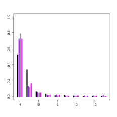
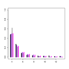
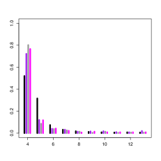
In all scenarios, we performed N=500𝑁500N=500 replications, the sample size was n=100𝑛100n=100 and we used cubic splines with equally spaced knots for all nonparametric components. For numerical simplicity, we also chose the same number of terms in the spline approximation for each additive component, that is, kj=ksubscript𝑘𝑗𝑘k_{j}=k for all j𝑗j. As in He et al. (2002), the common number of elements in the basis k𝑘k varies between max{n1/5/2;4}superscript𝑛1524\max\{n^{1/5}/2;4\} and 8+2n1/582superscript𝑛158+2n^{1/5}, which for the sample size considered leads to 4k134𝑘134\leq k\leq 13. To select the basis dimension, we minimized the RBIC𝑅𝐵𝐼𝐶RBIC criteria defined in (8) over the set {4,,13}413\{4,\dots,13\} with the same ρ𝜌\rho–function considered in the estimation step. Hence, for the robust estimator, the ρ𝜌\rho–function in (8) is the Tukey’s bisquare loss function with tuning constant c1=4.685subscript𝑐14.685c_{1}=4.685, while for the classical estimator, ρ(t)=t2𝜌𝑡superscript𝑡2\rho(t)=t^{2}. Note that for the classical procedure no scale estimator is needed.

The samples {(Yi,𝐙it,𝐗it)t}i=1nsuperscriptsubscriptsuperscriptsubscript𝑌𝑖superscriptsubscript𝐙𝑖tsuperscriptsubscript𝐗𝑖tt𝑖1𝑛\left\{(Y_{i},\mathbf{Z}_{i}^{\mbox{\footnotesize\sc t}},\mathbf{X}_{i}^{\mbox{\footnotesize\sc t}})^{\mbox{\footnotesize\sc t}}\right\}_{i=1}^{n} are generated with the same distribution as (Y,𝐙t,𝐗t)tsuperscript𝑌superscript𝐙tsuperscript𝐗tt(Y,\mathbf{Z}^{\mbox{\footnotesize\sc t}},\mathbf{X}^{\mbox{\footnotesize\sc t}})^{\mbox{\footnotesize\sc t}}, 𝐗=(X1,X2)t2𝐗superscriptsubscript𝑋1subscript𝑋2tsuperscript2\mathbf{X}=(X_{1},X_{2})^{\mbox{\footnotesize\sc t}}\in\mathbb{R}^{2}, 𝐙=(Z1,Z2)t2𝐙superscriptsubscript𝑍1subscript𝑍2tsuperscript2\mathbf{Z}=(Z_{1},Z_{2})^{\mbox{\footnotesize\sc t}}\in\mathbb{R}^{2}. In all cases, the response and the covariates are related through the partially linear additive model

Y=μ+βt𝐙+η1(X1)+η2(X2)+σε,𝑌𝜇superscript𝛽t𝐙subscript𝜂1subscript𝑋1subscript𝜂2subscript𝑋2𝜎𝜀Y=\mu+\beta^{\mbox{\footnotesize\sc t}}\mathbf{Z}+\eta_{1}(X_{1})+\eta_{2}(X_{2})+\sigma\,\varepsilon\,,

with β=(β1,β2)t=(3,3)t𝛽superscriptsubscript𝛽1subscript𝛽2tsuperscript33t\beta=(\beta_{1},\beta_{2})^{\mbox{\footnotesize\sc t}}=(3,3)^{\mbox{\footnotesize\sc t}}, μ=0𝜇0\mu=0, σ=0.2𝜎0.2\sigma=0.2, η1(x1)=2sin(πx1)4/πsubscript𝜂1subscript𝑥12𝜋subscript𝑥14𝜋\eta_{1}(x_{1})=2\sin(\pi x_{1})-{4}/{\pi} and η2(x2)=ex2(e1)subscript𝜂2subscript𝑥2superscript𝑒subscript𝑥2𝑒1\eta_{2}(x_{2})=e^{x_{2}}-(e-1), so that 01η1(x)𝑑x=01η2(x)𝑑x=0superscriptsubscript01subscript𝜂1𝑥differential-d𝑥superscriptsubscript01subscript𝜂2𝑥differential-d𝑥0\int_{0}^{1}\eta_{1}(x)\,dx=\int_{0}^{1}\eta_{2}(x)\,dx=0. Six possible models combining different choices for covariates distributions were studied. For all models X1subscript𝑋1X_{1} and X2subscript𝑋2X_{2} have marginal uniform distribution but different correlation between the covariates are allowed. In Models 4 to 6, Z1subscript𝑍1Z_{1} and Z2subscript𝑍2Z_{2} have a discrete distribution while in Models 1 to 3, they correspond to continuous random variables. For clean samples, denoted from now on as C0subscript𝐶0C_{0}, the errors distribution is εN(0,1)similar-to𝜀𝑁01\varepsilon\sim N(0,1) and the considered models for the covariates distribution are

  • Model 1: Z1,Z2,X1subscript𝑍1subscript𝑍2subscript𝑋1Z_{1},Z_{2},X_{1} and X2subscript𝑋2X_{2} are i.i.d. 𝒰(0,1)𝒰01\mathcal{U}(0,1).

  • Model 2: Z1,Z2,X1subscript𝑍1subscript𝑍2subscript𝑋1Z_{1},Z_{2},X_{1} and X2subscript𝑋2X_{2} have marginal 𝒰(0,1)𝒰01\mathcal{U}(0,1) distribution, X1subscript𝑋1X_{1} and Z1subscript𝑍1Z_{1} have correlation 0.70.70.7, while Z2subscript𝑍2Z_{2} and X2subscript𝑋2X_{2} independent and independent of Z1subscript𝑍1Z_{1} and X1subscript𝑋1X_{1}.

  • Model 3: X1subscript𝑋1X_{1} and X2subscript𝑋2X_{2} are i.i.d. 𝒰(0,1)𝒰01\mathcal{U}(0,1) and we defined Z1=X1+X22+u1subscript𝑍1subscript𝑋1superscriptsubscript𝑋22subscript𝑢1Z_{1}=X_{1}+X_{2}^{2}+u_{1}, Z2={exp(X1)1}/2+u2subscript𝑍2subscript𝑋112subscript𝑢2Z_{2}=\{\exp(X_{1})-1\}/2+u_{2}, where u1subscript𝑢1u_{1} and u2subscript𝑢2u_{2} i.i.d. ujN(0,(0.1)2)similar-tosubscript𝑢𝑗𝑁0superscript0.12u_{j}\sim N(0,(0.1)^{2}).

  • Model 4: X1subscript𝑋1X_{1} and X2subscript𝑋2X_{2} are i.i.d. with distribution 𝒰(0,1)𝒰01\mathcal{U}(0,1), Z1=W1/3subscript𝑍1subscript𝑊13Z_{1}=W_{1}/3 and Z2=W2/5subscript𝑍2subscript𝑊25Z_{2}=W_{2}/5 where W1Bi(3,1/2)similar-tosubscript𝑊1𝐵𝑖312W_{1}\sim Bi(3,1/2) and W2Bi(5,1/5)similar-tosubscript𝑊2𝐵𝑖515W_{2}\sim Bi(5,1/5) are independent of each other.

  • Model 5: X1subscript𝑋1X_{1} and X2subscript𝑋2X_{2} are i.i.d. Xj𝒰(0,1)similar-tosubscript𝑋𝑗𝒰01X_{j}\sim\mathcal{U}(0,1), Z1=W1/10subscript𝑍1subscript𝑊110Z_{1}=W_{1}/10 and Z2=W2/10subscript𝑍2subscript𝑊210Z_{2}=W_{2}/10 with (W1,W2,W3)(10,1/4,1/2,1/4)similar-tosubscript𝑊1subscript𝑊2subscript𝑊310141214(W_{1},W_{2},W_{3})\sim\mathcal{M}(10,1/4,1/2,1/4), that is, having a multinomial distribution, besides X1,X2subscript𝑋1subscript𝑋2X_{1},X_{2} and (W1,W2,W3)subscript𝑊1subscript𝑊2subscript𝑊3(W_{1},W_{2},W_{3}) are independent.

  • Model 6: X1subscript𝑋1X_{1} and X2subscript𝑋2X_{2} are i.i.d. Xj𝒰(0,1)similar-tosubscript𝑋𝑗𝒰01X_{j}\sim\mathcal{U}(0,1), Z1=W1/5subscript𝑍1subscript𝑊15Z_{1}=W_{1}/5 with W1Bi(5,1/4)similar-tosubscript𝑊1𝐵𝑖514W_{1}\sim Bi(5,1/4), X1,X2subscript𝑋1subscript𝑋2X_{1},X_{2} and W1subscript𝑊1W_{1} are independent. Moreover, Z2=(1/2){I(0;2/3)(X1)+W}subscript𝑍212subscript𝐼023subscript𝑋1𝑊Z_{2}=(1/2)\left\{I_{(0;2/3)}(X_{1})+W\right\} with WBi(1,1/2)similar-to𝑊𝐵𝑖112W\sim Bi(1,1/2) independent of X1subscript𝑋1X_{1}.

Note that all considered models satisfy the additivity required in assumption N3. However, under Model 6, h2(𝐱)=(1/2)I(0;2/3)(x1)+(1/4)superscriptsubscript2𝐱12subscript𝐼023subscript𝑥114h_{2}^{*}(\mathbf{x})=(1/2)I_{(0;2/3)}(x_{1})+(1/4) is not a smooth function.

To study the effect of atypical data on the estimators, we considered three contamination schemes which are described as

  • C1subscript𝐶1C_{1}: εi0.9N(0,1)+0.1N(0,100)similar-tosubscript𝜀𝑖0.9𝑁010.1𝑁0100\varepsilon_{i}\sim 0.9N(0,1)+0.1N(0,100).

  • C2subscript𝐶2C_{2}: ui0.85N(0,σ2)+0.15N(15,0.12)similar-tosubscript𝑢𝑖0.85𝑁0superscript𝜎20.15𝑁15superscript0.12u_{i}\sim 0.85N(0,\sigma^{2})+0.15N(15,0.1^{2}) where ui=σεisubscript𝑢𝑖𝜎subscript𝜀𝑖u_{i}=\sigma\varepsilon_{i}.

  • C3subscript𝐶3C_{3}: We divided the square [0,1]×[0,1]0101[0,1]\times[0,1] into 9 equally-sized quadrants as shown in Figure 1. In this scenario the errors are not contaminated, that is, εiN(0,1)similar-tosubscript𝜀𝑖𝑁01\varepsilon_{i}\sim N(0,1) but artificially 9 observations were modified in such a way that (Z1i,Z2i)t=(20,20)tsuperscriptsubscript𝑍1𝑖subscript𝑍2𝑖tsuperscript2020t(Z_{1i},Z_{2i})^{\mbox{\footnotesize\sc t}}=(20,20)^{\mbox{\footnotesize\sc t}} and its related pair (X1i,X2i)tsuperscriptsubscript𝑋1𝑖subscript𝑋2𝑖t(X_{1i},X_{2i})^{\mbox{\footnotesize\sc t}} of covariates belonged to a different quadrant in the square [0,1]×[0,1]0101[0,1]\times[0,1].

Contaminations C1subscript𝐶1C_{1} and C2subscript𝐶2C_{2} correspond to vertical outliers and it is expected that they will affect mainly the estimation of μ𝜇\mu and eventually that of the additive components. In particular, C1subscript𝐶1C_{1} corresponds to a 10%percent1010\% of the errors with a larger variance and will affect mainly the mean square error and not the bias of the estimates. In contrast, scenario C2subscript𝐶2C_{2} corresponds to an asymmetric gross error model in which a 15%percent1515\% of the errors are shifted in order to produce “vertical outliers” and will have more effect on the bias. In contrast, contamination C3subscript𝐶3C_{3} aims to affect the regression parameter also through the high leverage points introduced. Figure 1 shows the 100 pairs of 𝐗isubscript𝐗𝑖\mathbf{X}_{i} for one sample with X1subscript𝑋1X_{1} and X2subscript𝑋2X_{2} following a 𝒰(0,1)𝒰01\mathcal{U}(0,1) distribution. The solid blue circles correspond to the covariates 𝐗isubscript𝐗𝑖\mathbf{X}_{i} where 𝐙isubscript𝐙𝑖\mathbf{Z}_{i} has been contaminated. When no generated data points 𝐗isubscript𝐗𝑖\mathbf{X}_{i} were found in a quadrant, the observation 𝐙isubscript𝐙𝑖\mathbf{Z}_{i} was not contaminated, so the total amount of contaminated observations was less than 9.

Refer to caption
Figure 1: Scatter plot of the covariates (X1i,X2i)tsuperscriptsubscript𝑋1𝑖subscript𝑋2𝑖t(X_{1i},X_{2i})^{\mbox{\footnotesize\sc t}} corresponding to one of the samples contaminated according to scenario C3subscript𝐶3C_{3}. The solid circles indicate observations where (Z1i,Z2i)tsuperscriptsubscript𝑍1𝑖subscript𝑍2𝑖t(Z_{1i},Z_{2i})^{\mbox{\footnotesize\sc t}} is contaminated.

To study how the outliers affect the selection of the basis dimension, Figures 2 and 3 show the plots of the proportion of times that the value k𝑘k is selected by the BIC𝐵𝐼𝐶BIC criterion, under Models 3 and 4, respectively. Black bars correspond to the no contamination setting C0subscript𝐶0C_{0}, while purple, grey and magenta ones to the contamination settings C1subscript𝐶1C_{1}, C2subscript𝐶2C_{2} and C3subscript𝐶3C_{3}, respectively. The sensitivity to outliers of the classical BIC𝐵𝐼𝐶BIC criterion is reflected through the performance of the support of the selected basis dimension which is more concentrated at 4 for contaminated data. In contrast, when using the robust procedure combined with the robust BIC𝐵𝐼𝐶BIC all bars have similar heights showing the stability of the selection method. Note that for the MMlimit-from𝑀𝑀MM-estimators, only under C2subscript𝐶2C_{2}, dimension k=4𝑘4k=4 is selected more frequently than under C0subscript𝐶0C_{0}. It is also worth mentioning that the results reported in Figures 2 and 3 illustrate that, for clean samples, both the classical and the robust BIC𝐵𝐼𝐶BIC lead to similar choices for the basis dimension.

ls mm
Refer to caption Refer to caption
Figure 2: Plots of the proportion of the number of basis selected under Model 3. The black bars correspond to C0subscript𝐶0C_{0}, while the purple, grey and magenta ones to contaminations C1subscript𝐶1C_{1}, C2subscript𝐶2C_{2} and C3subscript𝐶3C_{3}, respectively.
ls mm
Refer to caption Refer to caption
Figure 3: Plots of the proportion of the number of basis selected under Model 4. The black bars correspond to C0subscript𝐶0C_{0}, while the purple, grey and magenta ones to contaminations C1subscript𝐶1C_{1}, C2subscript𝐶2C_{2} and C3subscript𝐶3C_{3}, respectively.

To evaluate the behaviour of the additive component estimators, we measured the performance of an estimator f^^𝑓\widehat{f} of a general function f:[0,1]:𝑓01f:[0,1]\to\mathbb{R} approximating the integrated squared error (ise) over an equally spaced grid of points {t}=1Msuperscriptsubscriptsubscript𝑡1𝑀\{t_{\ell}\}_{\ell=1}^{M}, 0t1<<tM10subscript𝑡1subscript𝑡𝑀10\leq t_{1}<\dots<t_{M}\leq 1 with M=1000𝑀1000M=1000, that is,

ise=1Ms=1M(f(ts)f^(ts))2.ise1𝑀superscriptsubscript𝑠1𝑀superscript𝑓subscript𝑡𝑠^𝑓subscript𝑡𝑠2\mbox{{ise}}=\frac{1}{M}\sum_{s=1}^{M}\left(f(t_{s})-\widehat{f}(t_{s})\right)^{2}\,.

Taking into account that a few large values of the ise may have a huge impact on its mean over replications and to prevent us for this distorted effect, instead of the mean integrated square error we considered two measures less affected by extreme values: the median of the ise, denoted medise and the mean of the ise obtained after trimming the 5% largest values labelled 5%-mise. The obtained results for the ise are given in Table 1.

Model 1 Model 2 Model 3 Model 4 Model 5 Model 6
ls mm ls mm ls mm ls mm ls mm ls mm
C0subscript𝐶0C_{0} 5%-mise 0.002 0.003 0.003 0.003 0.007 0.008 0.002 0.003 0.002 0.003 0.003 0.003
medise 0.002 0.002 0.002 0.003 0.005 0.006 0.002 0.002 0.002 0.002 0.003 0.003
\cdashline2-15 C1subscript𝐶1C_{1} 5%-mise 0.019 0.003 0.023 0.004 0.081 0.009 0.019 0.003 0.019 0.003 0.022 0.004
η1subscript𝜂1\eta_{1} medise 0.014 0.003 0.018 0.003 0.056 0.007 0.014 0.003 0.014 0.003 0.016 0.003
\cdashline2-15 C2subscript𝐶2C_{2} 5%-mise 1.175 0.003 1.484 0.003 4.866 0.008 1.127 0.003 1.147 0.003 1.432 0.003
medise 0.920 0.003 1.254 0.003 3.561 0.006 0.870 0.003 0.855 0.003 1.129 0.003
\cdashline2-15 C3subscript𝐶3C_{3} 5%-mise 0.063 0.003 0.660 0.004 2.553 0.009 0.038 0.003 0.009 0.003 0.281 0.003
medise 0.054 0.003 0.664 0.003 2.564 0.007 0.031 0.003 0.008 0.003 0.280 0.003
C0subscript𝐶0C_{0} 5%-mise 0.002 0.002 0.002 0.002 0.005 0.006 0.002 0.002 0.002 0.002 0.002 0.002
medise 0.001 0.002 0.002 0.002 0.003 0.004 0.001 0.002 0.001 0.002 0.002 0.002
\cdashline2-15 C1subscript𝐶1C_{1} 5%-mise 0.018 0.003 0.019 0.003 0.051 0.006 0.018 0.003 0.018 0.003 0.017 0.003
η2subscript𝜂2\eta_{2} medise 0.012 0.002 0.013 0.002 0.035 0.005 0.013 0.002 0.012 0.002 0.012 0.002
\cdashline2-15 C2subscript𝐶2C_{2} 5%-mise 1.282 0.002 1.256 0.002 3.470 0.006 1.244 0.002 1.231 0.002 1.271 0.002
medise 1.008 0.002 0.949 0.002 2.713 0.004 1.001 0.002 0.983 0.002 1.000 0.002
\cdashline2-15 C3subscript𝐶3C_{3} 5%-mise 0.063 0.002 0.046 0.002 0.793 0.006 0.038 0.002 0.009 0.002 0.047 0.002
medise 0.051 0.002 0.037 0.002 0.802 0.004 0.031 0.002 0.007 0.002 0.039 0.002
Table 1: Summary measures for the additive components estimates η^1subscript^𝜂1\widehat{\eta}_{1} and η^2subscript^𝜂2\widehat{\eta}_{2} based on the ise. The classical and robust procedures are labelled ls and mm, respectively.

Note that the ise is non-negative and expected to have a skewed distribution, for that reason, Figures 4 and 5 present skewed-adjusted boxplots, as defined in Hubert and Vandervieren (2008), to display the obtained ise results for the estimates of η1subscript𝜂1\eta_{1} and η2subscript𝜂2\eta_{2}, respectively, under Model 1. The red and blue boxes correspond to the classical and robust procedures, respectively. Similarly, Figures 6 and 7 contain the skewed-adjusted boxplots for the estimates of η1subscript𝜂1\eta_{1} and η2subscript𝜂2\eta_{2}, respectively, under Model 6.

Model 1
C0subscript𝐶0C_{0} C1subscript𝐶1C_{1}
Refer to caption Refer to caption
C2subscript𝐶2C_{2} C3subscript𝐶3C_{3}
Refer to caption Refer to caption
Figure 4: Boxplots of the ise values for estimating the additive function η1subscript𝜂1\eta_{1} for each contamination setting under Model 1, for the classical fit (in red) and for the robust fit (in blue).
Model 1
C0subscript𝐶0C_{0} C1subscript𝐶1C_{1}
Refer to caption Refer to caption
C2subscript𝐶2C_{2} C3subscript𝐶3C_{3}
Refer to caption Refer to caption
Figure 5: Boxplots of the ise values for estimating the additive function η2subscript𝜂2\eta_{2} for each contamination setting under Model 1, for the classical fit (in red) and for the robust fit (in blue).
Model 6
C0subscript𝐶0C_{0} C1subscript𝐶1C_{1}
Refer to caption Refer to caption
C2subscript𝐶2C_{2} C3subscript𝐶3C_{3}
Refer to caption Refer to caption
Figure 6: Boxplots of the ise values for estimating the additive function η1subscript𝜂1\eta_{1} for each contamination setting under Model 6, for the classical fit (in red) and for the robust fit (in blue).
Model 6
C0subscript𝐶0C_{0} C1subscript𝐶1C_{1}
Refer to caption Refer to caption
C2subscript𝐶2C_{2} C3subscript𝐶3C_{3}
Refer to caption Refer to caption
Figure 7: Boxplots of the ise values for estimating the additive function η2subscript𝜂2\eta_{2} for each contamination setting under Model 6, for the classical fit (in red) and for the robust fit (in blue).
Model 1
ls mm
η1subscript𝜂1\eta_{1} Refer to caption Refer to caption
η2subscript𝜂2\eta_{2} Refer to caption Refer to caption
Figure 8: Boxplots of the ise values obtained for the classical and robust estimations of the additive functions η1subscript𝜂1\eta_{1} and η2subscript𝜂2\eta_{2} for each contamination setting under Model 1.
Model 6
ls mm
η1subscript𝜂1\eta_{1} Refer to caption Refer to caption
η2subscript𝜂2\eta_{2} Refer to caption Refer to caption
Figure 9: Boxplots of the ise values obtained for the classical and robust estimations of the additive functions η1subscript𝜂1\eta_{1} and η2subscript𝜂2\eta_{2} for each contamination setting under Model 6.

As seen in Table 1, for clean samples, both classical and robust procedures present a similar behaviour. This fact is also reflected in the boxplots of the ise presented in Figures 4 to 7. Note that, due to the efficiency loss, the ise for the robust method are slightly larger and show more wider boxes than when considering the classical procedure. In contrast, under the contamination schemes considered, the obtained values of the ise for the classical estimates are considerably enlarged which respect to those obtained for the robust procedure. Furthermore, the boxplots under C1subscript𝐶1C_{1} to C3subscript𝐶3C_{3} for the robust method are shifted towards 00 with respect to those of the classical one. To see this effect, Figures 8 and 9 shows the same adjusted boxplots as parallel ones, for Models 1 and 6, respectively. The colours black, purple, grey and magenta identify the boxplots for the contamination settings C0subscript𝐶0C_{0}, C1subscript𝐶1C_{1}, C2subscript𝐶2C_{2} and C3subscript𝐶3C_{3}, respectively. The stability of the robust procedure is reflected in the right panel of Figures 8 and 9, since all the boxplots are very similar. On the contrary, when observing the left panel, we appreciate the sensitivity of the classical fits, in particular under C2subscript𝐶2C_{2} where the ise values are extremely large leading to boxplots which are much higher than the other ones. One of the reason of observing large values for the ise is that it may be heavily influenced by numerical errors at or near the boundaries of the grid, that is why, following He and Shi (1998), we consider a trimmed version of the ise computed without the q𝑞q first and last points on the grid, that is,

isetrsubscriptisetr\displaystyle\mbox{{ise}}_{\mbox{\footnotesize\sc tr}} =\displaystyle= 1M2qs=q+1Mq(f(ts)f^(ts))2,1𝑀2𝑞superscriptsubscript𝑠𝑞1𝑀𝑞superscript𝑓subscript𝑡𝑠^𝑓subscript𝑡𝑠2\displaystyle\frac{1}{M-2q}\sum_{s=q+1}^{M-q}\left(f(t_{s})-\widehat{f}(t_{s})\right)^{2}\,,

We chose q=[M×0.05]𝑞delimited-[]𝑀0.05q=[M\times 0.05] which uses the central 90% interior points in the grid. Table 2 reports the trimmed mean and the median of the isetrsubscriptisetr\mbox{{ise}}_{\mbox{\footnotesize\sc tr}} denoted misetrtr{}_{\mbox{\footnotesize\sc tr}} and medisetrtr{}_{\mbox{\footnotesize\sc tr}}, respectively.

Model 1 Model 2 Model 3 Model 4 Model 5 Model 6
ls mm ls mm ls mm ls mm ls mm ls mm
C0subscript𝐶0C_{0} misetrtr{}_{\mbox{\footnotesize\sc tr}} 0.002 0.007 0.002 0.003 0.007 0.008 0.002 0.002 0.002 0.006 0.002 0.003
medisetrtr{}_{\mbox{\footnotesize\sc tr}} 0.002 0.002 0.002 0.002 0.004 0.004 0.002 0.002 0.002 0.002 0.002 0.002
\cdashline2-15 C1subscript𝐶1C_{1} misetrtr{}_{\mbox{\footnotesize\sc tr}} 0.019 0.003 0.023 0.003 0.082 0.009 0.019 0.003 0.018 0.003 0.022 0.003
η1subscript𝜂1\eta_{1} medisetrtr{}_{\mbox{\footnotesize\sc tr}} 0.010 0.002 0.013 0.002 0.043 0.005 0.010 0.002 0.010 0.002 0.013 0.002
\cdashline2-15 C2subscript𝐶2C_{2} misetrtr{}_{\mbox{\footnotesize\sc tr}} 1.104 0.002 1.335 0.003 4.845 0.008 1.052 0.002 1.063 0.002 1.351 0.003
medise 0.612 0.002 0.847 0.002 2.761 0.005 0.583 0.002 0.580 0.002 0.819 0.002
\cdashline2-15 C3subscript𝐶3C_{3} misetrtr{}_{\mbox{\footnotesize\sc tr}} 0.057 0.002 0.505 0.003 2.068 0.009 0.035 0.002 0.008 0.002 0.269 0.003
medisetrtr{}_{\mbox{\footnotesize\sc tr}} 0.037 0.002 0.489 0.002 2.058 0.005 0.021 0.002 0.005 0.002 0.252 0.002
C0subscript𝐶0C_{0} misetrtr{}_{\mbox{\footnotesize\sc tr}} 0.002 0.011 0.002 0.002 0.005 0.006 0.002 0.002 0.002 0.002 0.002 0.002
medise 0.001 0.001 0.001 0.002 0.003 0.001 0.001 0.001 0.001 0.001 0.001 0.001
\cdashline2-15 C1subscript𝐶1C_{1} misetrtr{}_{\mbox{\footnotesize\sc tr}} 0.018 0.002 0.018 0.003 0.050 0.006 0.018 0.004 0.017 0.002 0.017 0.003
η2subscript𝜂2\eta_{2} medisetrtr{}_{\mbox{\footnotesize\sc tr}} 0.009 0.002 0.010 0.001 0.026 0.004 0.010 0.002 0.009 0.001 0.008 0.002
\cdashline2-15 C2subscript𝐶2C_{2} misetrtr{}_{\mbox{\footnotesize\sc tr}} 1.182 0.041 1.219 0.002 3.357 0.005 1.148 0.002 1.134 0.007 1.206 0.002
medisetrtr{}_{\mbox{\footnotesize\sc tr}} 0.707 0.001 0.679 0.001 2.075 0.003 0.679 0.001 0.704 0.001 0.708 0.001
\cdashline2-15 C3subscript𝐶3C_{3} misetrtr{}_{\mbox{\footnotesize\sc tr}} 0.058 0.068 0.043 0.002 0.651 0.006 0.036 0.002 0.008 0.002 0.042 0.002
medisetrtr{}_{\mbox{\footnotesize\sc tr}} 0.034 0.001 0.026 0.001 0.645 0.004 0.021 0.001 0.005 0.001 0.030 0.001
Table 2: Summary measures for the additive components estimates η^1subscript^𝜂1\widehat{\eta}_{1} and η^2subscript^𝜂2\widehat{\eta}_{2} based on the isetrsubscriptisetr\mbox{{ise}}_{\mbox{\footnotesize\sc tr}}. The classical and robust procedures are labelled ls and mm, respectively.

Under C0subscript𝐶0C_{0}, the trimmed mise and medise of the classical estimators of the additive components and regression function are equal or very similar to those of the robust ones. Tables 1 and 2 and also Figures 4 to 9 illustrate the damage caused to the classical estimators by contamination C2subscript𝐶2C_{2}. The ise and the trimmed ise of the least squares estimators of η1subscript𝜂1\eta_{1} and η2subscript𝜂2\eta_{2}, across all models, are consistently higher than those of the robust estimators. In particular, the 5%-mise and the misetrtr{}_{\mbox{\footnotesize\sc tr}} of the classical procedure are more than 400 times those obtained with the robust method in all models. The other two contaminations also affect the classical estimators of the additive components but in a smaller degree since the ratio between the summary measure obtained for the classical and robust estimates is close to 4. In particular, vertical outliers have a low impact on the least squares estimators of η1subscript𝜂1\eta_{1} and η2subscript𝜂2\eta_{2} only increasing their variability but not affecting their bias as it will be shown below in the functional boxplots of the estimated curves. In contrast to the described behaviour of the least squares method, our robust proposal provides more reliable estimates of the additive components which are almost unaffected by the different types of outliers, see Figures 8 and 9.

To illustrate the performance of the estimated curves η^1subscript^𝜂1\widehat{\eta}_{1} and η^2subscript^𝜂2\widehat{\eta}_{2}, Figure 11 displays their functional boxplots when using the classical and robust procedures, under Model 6. As it is well-known when using splines, for both classical and robust fits, estimating problems may arise near the boundaries, for that reason, we show here the different estimates η^1subscript^𝜂1\widehat{\eta}_{1} and η^2subscript^𝜂2\widehat{\eta}_{2} evaluated on a grid of 100 equispaced points within the interval [0.05,0.95]0.050.95[0.05,0.95]. Functional boxplots, introduced by Sun and Genton (2011), are useful to visualize a collection of curves. The area in purple represents the 50% inner band of curves, the dotted red lines correspond to outlying curves and the blue lines to the whiskers while the black line indicates the deepest function. The true functions is shown in solid green line in all plots. As it is expected, for clean samples, box and whiskers for the robust fits are slightly larger than those obtained by the classical approach. However, for contamination settings C1subscript𝐶1C_{1} to C3subscript𝐶3C_{3} the general structure of the additive functions have been better captured by the robust fit noted on narrower envelops In particular, when estimating η1subscript𝜂1\eta_{1}, contamination C3subscript𝐶3C_{3} distorts the classical estimators since the true function η1subscript𝜂1\eta_{1} is not contained in the region containing the 50% central curves.

ls mm
C0subscript𝐶0C_{0} Refer to caption Refer to caption
C1subscript𝐶1C_{1} Refer to caption Refer to caption
C2subscript𝐶2C_{2} Refer to caption Refer to caption
C3subscript𝐶3C_{3} Refer to caption Refer to caption
Figure 10: Functional boxplots of the estimated additive functions η1subscript𝜂1\eta_{1} obtained by the classical and robust fit under Model 6. The solid green line corresponds to the true function η1subscript𝜂1\eta_{1}.
ls mm
C0subscript𝐶0C_{0} Refer to caption Refer to caption
C1subscript𝐶1C_{1} Refer to caption Refer to caption
C2subscript𝐶2C_{2} Refer to caption Refer to caption
C3subscript𝐶3C_{3} Refer to caption Refer to caption
Figure 11: Functional boxplots of the estimated additive functions η2subscript𝜂2\eta_{2} obtained by the classical and robust fit under Model 6. The solid green line corresponds to the true function η2subscript𝜂2\eta_{2}.

For the estimators of the regression parameter 𝜷𝜷\beta, we considered as summary measures the bias, standard deviation and the mean square error of each component, denoted bias, sd and mse, respectively. Tables 3 and 4 report the results obtained for the estimators of β1subscript𝛽1\beta_{1} and β2subscript𝛽2\beta_{2}, respectively.

Model 1 Model 2 Model 3 Model 4 Model 5 Model 6
ls mm ls mm ls mm ls mm ls mm ls mm
bias 0.000 -0.002 0.000 0.002 -0.018 -0.016 0.000 -0.001 -0.007 -0.002 0.002 0.001
C0subscript𝐶0C_{0} sd 0.075 0.079 0.098 0.106 0.201 0.214 0.074 0.078 0.199 0.209 0.109 0.113
mse 0.006 0.006 0.010 0.011 0.040 0.046 0.005 0.006 0.040 0.044 0.012 0.013
bias -0.010 -0.004 -0.006 0.003 -0.010 -0.020 -0.011 -0.004 -0.060 -0.003 -0.013 0.001
C1subscript𝐶1C_{1} sd 0.245 0.086 0.334 0.113 0.679 0.226 0.251 0.087 0.623 0.226 0.386 0.123
mse 0.060 0.007 0.111 0.013 0.461 0.051 0.063 0.008 0.391 0.051 0.149 0.015
bias -0.087 -0.002 0.068 0.006 0.009 -0.021 -0.080 -0.001 -0.269 0.003 0.049 0.001
C2subscript𝐶2C_{2} sd 1.879 0.085 2.811 0.111 5.618 0.223 1.869 0.084 5.113 0.223 2.951 0.118
mse 3.530 0.007 7.888 0.012 31.495 0.050 3.491 0.007 26.168 0.050 8.693 0.014
bias -2.989 -0.002 -3.963 0.004 -2.975 -0.010 -1.629 -0.002 -3.287 -0.005 -3.884 0.001
C3subscript𝐶3C_{3} sd 0.231 0.082 0.272 0.111 0.317 0.224 0.287 0.080 0.184 0.218 0.270 0.119
mse 8.986 0.007 15.776 0.012 8.948 0.050 2.737 0.006 10.839 0.048 15.155 0.014
Table 3: Bias, standard deviations and mean square errors for the estimates of the first coordinate β1subscript𝛽1\beta_{1} of 𝜷𝜷\beta. The classical and robust procedures are labelled ls and mm, respectively.
Model 1 Model 2 Model 3 Model 4 Model 5 Model 6
ls mm ls mm ls mm ls mm ls mm ls mm
bias 0.002 0.001 0.002 0.001 0.002 0.003 0.002 0.001 -0.006 -0.002 0.011 0.007
C0subscript𝐶0C_{0} sd 0.076 0.081 0.075 0.078 0.210 0.215 0.123 0.128 0.172 0.179 0.087 0.091
mse 0.006 0.007 0.006 0.006 0.044 0.046 0.015 0.016 0.030 0.032 0.008 0.008
bias -0.017 -0.001 -0.002 0.002 0.004 -0.002 -0.039 -0.005 -0.029 -0.004 0.024 0.012
C1subscript𝐶1C_{1} sd 0.239 0.088 0.233 0.086 0.709 0.236 0.391 0.143 0.560 0.196 0.267 0.101
mse 0.057 0.008 0.054 0.007 0.502 0.056 0.154 0.020 0.314 0.038 0.072 0.010
bias -0.051 -0.001 -0.035 0.001 -0.218 0.003 -0.166 -0.002 -0.274 0.004 -0.006 0.012
C2subscript𝐶2C_{2} sd 2.054 0.085 2.185 0.082 5.959 0.227 3.174 0.137 4.536 0.195 2.238 0.097
mse 4.214 0.007 4.766 0.007 35.491 0.052 10.080 0.019 20.605 0.038 5.001 0.010
bias -3.005 0.001 -2.033 0.003 -3.024 0.002 -4.346 0.001 -2.709 0.001 -2.097 0.010
C3subscript𝐶3C_{3} sd 0.231 0.081 0.272 0.081 0.309 0.225 0.283 0.131 0.187 0.184 0.277 0.094
mse 9.082 0.006 4.208 0.007 9.241 0.050 18.970 0.017 7.371 0.034 4.472 0.009
Table 4: Bias, standard deviations and mean square errors for the estimates of the second coordinate β2subscript𝛽2\beta_{2} of 𝜷𝜷\beta. The classical and robust procedures are labelled ls and mm, respectively.

As expected, for clean data sets, the classical and robust estimators of the regression parameter behave similarly (see Tables 3 and 4). When estimating the regression coefficient 𝜷𝜷\beta, the less efficient robust estimator naturally results in higher standard deviations, even though the mean square error is equal to that of the classical counterpart due to a bias reduction.

Regarding the performance of the estimates of 𝜷𝜷\beta under contamination, scenario C1subscript𝐶1C_{1} mainly affects the variability of the classical regression estimator (see Tables 3 and 4). This performance is related to the fact that the errors are still centered for this scheme but with a large dispersion. Finally, the high-leverage outliers introduced under C3subscript𝐶3C_{3} have a damaging effect on the classical estimators of 𝜷𝜷\beta that become completely uninformative, see Tables 3 and 4 and Figures 12 and 15, since the absolute bias is enlarged more than 800 times affecting the mean square error. In contrast, the proposed robust estimators show a very stable behaviour across all contamination and model settings. The bias and mean square error of the estimators of 𝜷𝜷\beta, reported in Tables 3 and 4, show that the robust procedure is highly resistant against the contamination scenarios considered here, even when bad high leverage points are introduced in the sample.

ls mm
Refer to caption Refer to caption
Figure 12: Plots of the mean over replications of |β^1β1|subscript^𝛽1subscript𝛽1|\widehat{\beta}_{1}-\beta_{1}| for each contamination setting (identified through colours in the legend) and for the different models (denoted M1 to M6 in the horizontal axis). The left panel corresponds to the classical procedure, while the right one to the robust method.

With the goal of analysing the outliers impact on the bias of the estimators of β1subscript𝛽1\beta_{1}, Figure 13 shows the mean over replications of the absolute bias |β^1β1|subscript^𝛽1subscript𝛽1|\widehat{\beta}_{1}-\beta_{1}|, under the six models considered. Again, red filled triangles and blue filled circles correspond to the classical and robust estimators, respectively. The harmful effect of contamination schemes C2subscript𝐶2C_{2} and C3subscript𝐶3C_{3} on the classical procedure may be appreciate on the plots. To facilitate the comparison across contaminations, Figure 12 reports the mean over replications of the absolute bias |β^1β1|subscript^𝛽1subscript𝛽1|\widehat{\beta}_{1}-\beta_{1}| but with all contamination settings in the same plot. The different sizes of the filled circles allow to appreciate that for the robust estimators the results are almost the same. As shown in Figures 12 and 13, the impact of outliers on the bias of the classical method is particularly high under scheme C3subscript𝐶3C_{3} which corresponds to high leverage points. In contrast, the robust procedure is stable providing reliable estimations. This effect is also visualized in Figure 14 that reports the mse values obtained when estimating β1subscript𝛽1\beta_{1}. As above, the red filled triangles correspond to the classical estimators, while the blue filled circles to the robust ones. Regarding the mse, as expected, for clean samples the classical and robust approaches lead to similar results, although they are slightly higher for the robust fit due to the lack of efficiency. On the other hand, for all models and contamination settings, the classical procedure leads to values of the mse that are much larger than those obtained by the robust one. The dramatic effect of contaminations on the classical estimators is more striking in the left panel of Figure 15 which present with different colours the contamination schemes and the six models in the horizontal axis. This Figure allows to appreciate that, while for the robust approach the obtained values are close to each other, for the classical one the mse values are much higher than those obtained for clean samples, specially when considering the contamination schemes C2subscript𝐶2C_{2} and C3subscript𝐶3C_{3}.

C0subscript𝐶0C_{0} C1subscript𝐶1C_{1}
Refer to caption Refer to caption
C2subscript𝐶2C_{2} C3subscript𝐶3C_{3}
Refer to caption Refer to caption
Figure 13: Plots of the mean over replications of |β^1β1|subscript^𝛽1subscript𝛽1|\widehat{\beta}_{1}-\beta_{1}|, for each contamination setting. The red filled triangles correspond to the classical estimator, while the blue circles to the robust ones.
C0subscript𝐶0C_{0} C1subscript𝐶1C_{1}
Refer to caption Refer to caption
C2subscript𝐶2C_{2} C3subscript𝐶3C_{3}
Refer to caption Refer to caption
Figure 14: Plots of the mse error obtained when estimating β1subscript𝛽1\beta_{1} for each contamination setting. The red filled triangles correspond to the classical estimator, while the blue circles to the robust ones.
ls mm
Refer to caption Refer to caption
Figure 15: Plots of the mse error obtained when estimating β1subscript𝛽1\beta_{1} for each contamination setting (identified through colours in the legend) and for the different models (denoted as M1 to M6 in the horizontal axis). The left panel corresponds to the classical procedure, while the right one to the robust method.

With respect to the estimation of the constant μ𝜇\mu, Table 5 reports the mean and standard deviation over replications of the classical and robust estimates, for all models and contamination settings. Besides, Figure 16 shows the mean over replications of estimation of the coefficient μ𝜇\mu for all the models and contamination settings considered. Red triangles and blue circles correspond to the classical and robust estimates, respectively. The true value of the parameter (μ=0𝜇0\mu=0) is shown using an horizontal gray line. Under C0subscript𝐶0C_{0}, the mean of the classical and robust estimates are similar, however, due to the loss of efficiency of the robust proposal, the standard deviation of the classical estimator is smaller than that of the robust one. Contamination scheme C1subscript𝐶1C_{1} do not affect the bias of the classical estimates but it enlarges its variability, while the robust proposal remains stable. The only exception is Model 3, where the robust procedure presents a larger bias, see also Figure 16. Under schemes C2subscript𝐶2C_{2} and C3subscript𝐶3C_{3}, the mean of the classical estimators is distorted under the six models (see Figure 16). Besides, the standard deviations of the classical estimators are also larger than those of the robust ones under these two contamination settings, specially under C2subscript𝐶2C_{2}, except for Model 1 and C3subscript𝐶3C_{3} where the variability is smaller for the classical procedure but with a huge bias making the estimates unreliable.

Model 1 Model 2 Model 3 Model 4 Model 5 Model 6
ls mm ls mm ls mm ls mm ls mm ls mm
mean -0.001 0.002 -0.001 -0.002 0.014 0.011 -0.001 -0.000 0.004 -0.001 -0.008 -0.006
C0subscript𝐶0C_{0} sd 0.058 0.107 0.064 0.070 0.183 0.196 0.049 0.052 0.123 0.130 0.059 0.061
mean 0.010 0.003 0.007 -0.004 0.007 0.017 0.009 0.005 0.025 0.003 -0.017 -0.008
C1subscript𝐶1C_{1} sd 0.188 0.069 0.211 0.076 0.641 0.207 0.166 0.064 0.398 0.139 0.198 0.070
mean 2.322 0.012 2.258 -0.005 2.348 0.015 2.326 0.001 2.448 0.000 2.244 -0.007
C2subscript𝐶2C_{2} sd 1.586 0.185 1.928 0.072 5.161 0.202 1.326 0.056 3.263 0.155 1.530 0.066
mean 2.988 0.010 2.995 -0.003 3.564 0.006 1.675 -0.000 2.174 0.001 2.183 -0.007
C3subscript𝐶3C_{3} sd 0.143 0.231 0.123 0.074 0.166 0.207 0.152 0.053 0.072 0.133 0.160 0.064
Table 5: Mean and standard deviations for the estimates of μ𝜇\mu. The classical and robust procedures are labelled ls and mm, respectively.
C0subscript𝐶0C_{0} C1subscript𝐶1C_{1}
Refer to caption Refer to caption
C2subscript𝐶2C_{2} C3subscript𝐶3C_{3}
Refer to caption Refer to caption
Figure 16: Plots of the mean over replications of μ^^𝜇\widehat{\mu}, for each contamination setting. The red filled triangles correspond to the classical estimator, while the blue circles to the robust ones.

6 Real data example

In this section, we analyse the airquality data set available in R which considers different variables to evaluate daily air quality in the New York region between May and September, 1973 (see Chambers et al., 1983). The goal of our analysis is to model the Ozone concentration (“O3subscript𝑂3O_{3}”, measured in ppb) using as explanatory variables: the month, the temperature, the wind speed and the solar radiation labelled “Month”, “Temp”, “Wind”, and “Solar.R”, respectively. Regarding these covariates the month is a categorical variable with categories going from 5 to 9, the other variables may be considered as continuous. Temperature is measured in Fahrenheit degrees, wind speed in mph and solar radiation in Langleys in the frequency band 4000-7700. We considered n=111𝑛111n=111 observations corresponding to cases that do not contain missing values neither in the response variable nor in the covariates.

As mentioned in Boente et al. (2017), Dengyi and Kawagochi (1986) and Lacour et al. (2006) report a positive correlation between the ozone concentration and temperature in the Antarctica during Spring and also, in France during the 2003 heat wave. Besides, Cleveland (1985) finds that the relationship between ozone concentration and wind speed is nonlinear, with higher wind speeds associated to lower concentrations of ozone. Atypical data have been previously detected in this data set. Effectively, Boente et al. (2017) used a robust fit to an additive model using as covariates “Temp”, “Wind”, and “Solar.R”, while Bianco and Spano (2019) consider a robust fit for an exponential growth model that aims to explain the ozone daily behaviour in terms of wind speed. For that reason, it is important to identify possible atypical observations and evaluate the behaviour of the robust and classical estimators when all the covariates described above are included in the model. We then consider the following partially linear additive model

O3=μ+𝜷tMonth+η1(Temp)+η2(Wind)+η3(Solar.R)+usubscript𝑂3𝜇superscript𝜷tMonthsubscript𝜂1Tempsubscript𝜂2Windsubscript𝜂3Solar.R𝑢O_{3}=\mu+\mbox{\boldmath$\beta$}^{\mbox{\footnotesize\sc t}}\mbox{Month}+\eta_{1}(\mbox{Temp})+\eta_{2}(\mbox{Wind})+\eta_{3}(\mbox{Solar.R})+u

where the errors u=σε𝑢𝜎𝜀u=\sigma\;\varepsilon are assumed to be independent, homoscedastic and with location parameter 0, Month=(d6,d7,d8,d9)t4absentsuperscriptsubscript𝑑6subscript𝑑7subscript𝑑8subscript𝑑9tsuperscript4=(d_{6},d_{7},d_{8},d_{9})^{\mbox{\footnotesize\sc t}}\in\mathbb{R}^{4} with d=1subscript𝑑1d_{\ell}=1 if the month is the limit-from\ell-th one and 0 otherwise, for =6,,969\ell=6,\dots,9, and 𝜷0=(β1,β2,β3,β4)t4subscript𝜷0superscriptsubscript𝛽1subscript𝛽2subscript𝛽3subscript𝛽4tsuperscript4\mbox{\boldmath$\beta$}_{0}=(\beta_{1},\beta_{2},\beta_{3},\beta_{4})^{\mbox{\footnotesize\sc t}}\in\mathbb{R}^{4}. With this notation 𝐙=Month𝐙Month\mathbf{Z}=\mbox{Month} and 𝐗=(X1,X2,X3)t=(Temp,Wind,Solar.R)t𝐗superscriptsubscript𝑋1subscript𝑋2subscript𝑋3tsuperscriptTempWindSolar.Rt\mathbf{X}=(X_{1},X_{2},X_{3})^{\mbox{\footnotesize\sc t}}=(\mbox{Temp},\mbox{Wind},\mbox{Solar.R})^{\mbox{\footnotesize\sc t}}.

To estimate the additive components, we use cubic Blimit-from𝐵B-splines. When estimating ηjsubscript𝜂𝑗\eta_{j}, the knots are taken as the /(k+1)100%𝑘1percent100\ell/(k+1)100\% quantiles, =1,,k1𝑘\ell=1,\dots,k, of the observed values of Xjsubscript𝑋𝑗X_{j}. Taking into account that n=111𝑛111n=111, the basis dimension k𝑘k varies between 4 and 13. Both the classical and the robust BIC𝐵𝐼𝐶BIC criteria introduced in (8) selected 555 terms to approximate the additive functions. The loss function and tuning constants were selected as in the simulation study.

From now on, we label with the subscripts cl and mm the estimators obtained through the classical and robust approach, respectively. The obtained estimates of μ𝜇\mu equal μ^ls=46.054subscript^𝜇ls46.054\widehat{\mu}_{\mbox{\scriptsize\sc ls}}=46.054 and μ^mm=40.651subscript^𝜇mm40.651\widehat{\mu}_{\mbox{\scriptsize\sc m}\mbox{\scriptsize\sc m}}=40.651, while those of 𝜷𝜷\beta are 𝜷^ls=(6.736,4.614,3.907,12.008)tsubscript^𝜷lssuperscript6.7364.6143.90712.008t\widehat{\mbox{\boldmath$\beta$}}_{\mbox{\scriptsize\sc ls}}=(-6.736,-4.614,3.907,-12.008)^{\mbox{\footnotesize\sc t}} and 𝜷^mm=(5.641,0.539,5.167,5.816)tsubscript^𝜷mmsuperscript5.6410.5395.1675.816t\widehat{\mbox{\boldmath$\beta$}}_{\mbox{\scriptsize\sc m}\mbox{\scriptsize\sc m}}=(-5.641,-0.539,5.167,-5.816)^{\mbox{\footnotesize\sc t}}. The presence of possible atypical data is suspected from the differences observed between these estimates. In particular, when considering the estimators of β2subscript𝛽2\beta_{2}, the classical procedure leads to an estimate which is almost 10 times larger than the robust one and the robust estimates of β4subscript𝛽4\beta_{4} are a half than those obtained with the classical approach. The estimators of ηjsubscript𝜂𝑗\eta_{j}, j=1,2,3𝑗123j=1,2,3 are shown in Figure 17 together with the partial residuals corresponding to the robust fit. Solid blue lines are used for the robust estimator and red dashed ones for the classical one. Even though the shape of the estimates corresponding to the solar radiation is similar for both the robust and classical method, differences are observed in the estimation of η1subscript𝜂1\eta_{1} and η2subscript𝜂2\eta_{2}. In particular, the classical estimate of the additive component related to temperature has a lower peak than the robust one for high values of temperature. Note that the obtained estimates of ηjsubscript𝜂𝑗\eta_{j} have a shape quite similar to that obtained in Boente et al. (2017) who considered an additive model and use a backfitting approach without including the variable month.

η^1subscript^𝜂1\widehat{\eta}_{1}                                          η^2subscript^𝜂2\widehat{\eta}_{2}                                          η^3subscript^𝜂3\widehat{\eta}_{3}

Refer to caption
Refer to caption
Refer to caption

Temp                                       Wind                                      Solar.R

Figure 17: Estimated curves for the classical (in red dashed lines) and robust (in blue solid lines) estimators.

To identify potential outliers in the data, we use a boxplot of the residuals obtained from the robust fit. This boxplot is displayed in Figure 18 and identifies as atypical the observations 23, 34, 53 and 77. These four observations were also detected in Boente et al. (2017). We then compute the classical estimators after removing these potential atypical data. As above, the number of knots was the same for all components and a classical BIC was used to select the basis dimension k𝑘k resulting in k=5𝑘5k=5. The dashed red lines in Figure 19 correspond to the classical fit computed without these possible atypical observations. The blue solid lines correspond to the robust estimators computed with the original data set. Blue points correspond to the partial residuals obtained by the robust fit, while the black points identify the partial residuals corresponding to the four observations detected as atypical. Note that the classical estimators computed without these potential outliers are very close to the robust ones. In other words, the robust estimator behaves similarly to the classical one if one were able to manually remove suspected outliers. Besides, the classical estimates of μ𝜇\mu and 𝜷𝜷\beta after removing the four outliers, denoted μ^ls(4)superscriptsubscript^𝜇ls4\widehat{\mu}_{\mbox{\scriptsize\sc ls}}^{(-4)} and 𝜷^ls(4)superscriptsubscript^𝜷ls4\widehat{\mbox{\boldmath$\beta$}}_{\mbox{\scriptsize\sc ls}}^{(-4)}, are equal to μ^ls(4)=39.374superscriptsubscript^𝜇ls439.374\widehat{\mu}_{\mbox{\scriptsize\sc ls}}^{(-4)}=39.374 and 𝜷^ls(4)=(4.920,0.126,6.475,5.558)tsuperscriptsubscript^𝜷ls4superscript4.9200.1266.4755.558t\widehat{\mbox{\boldmath$\beta$}}_{\mbox{\scriptsize\sc ls}}^{(-4)}=(-4.920,-0.126,6.475,-5.558)^{\mbox{\footnotesize\sc t}}. Even though there is a difference between the estimates of the second component of 𝜷𝜷\beta, μ^ls(4)superscriptsubscript^𝜇ls4\widehat{\mu}_{\mbox{\scriptsize\sc ls}}^{(-4)} and 𝜷^ls(4)superscriptsubscript^𝜷ls4\widehat{\mbox{\boldmath$\beta$}}_{\mbox{\scriptsize\sc ls}}^{(-4)} have values closer to μ^mmsubscript^𝜇mm\widehat{\mu}_{\mbox{\scriptsize\sc m}\mbox{\scriptsize\sc m}} and 𝜷^mmsubscript^𝜷mm\widehat{\mbox{\boldmath$\beta$}}_{\mbox{\scriptsize\sc m}\mbox{\scriptsize\sc m}} than to μ^lssubscript^𝜇ls\widehat{\mu}_{\mbox{\scriptsize\sc ls}} and 𝜷^lssubscript^𝜷ls\widehat{\mbox{\boldmath$\beta$}}_{\mbox{\scriptsize\sc ls}}.

To conclude the robust procedure leads to more reliable results automatically down–weighting potential outliers. It also allows to identify potential atypical observations and leads to estimated components ηjsubscript𝜂𝑗\eta_{j} that are almost identical to the classical ones when these detected outliers are removed.

Refer to caption
Figure 18: Boxplot of the residuals obtained using the robust fit.

η^1subscript^𝜂1\widehat{\eta}_{1}                                          η^2subscript^𝜂2\widehat{\eta}_{2}                                          η^3subscript^𝜂3\widehat{\eta}_{3}

Refer to caption
Refer to caption
Refer to caption

Temp                                       Wind                                      Solar.R

Figure 19: Estimated curves for ηjsubscript𝜂𝑗\eta_{j}, j=1,2,3𝑗123j=1,2,3. The red dashed line corresponds to the classical estimators after the atypical data have been removed. The blue solid line indicated the robust fit computed with the whole data set.

7 Final Comments

In this paper, we presented a procedure to robustly estimate the regression parameter and the additive components under a partially linear additive model. The method combines Blimit-from𝐵B-splines to smoothly estimate the additive components and MMlimit-from𝑀𝑀MM-estimators. The use of Blimit-from𝐵B-splines avoids the higher complexity of kernels methods which require backfitting or marginal integration combined with a profile approach, see, for instance, Li (2000) or Ma and Yan (2011) for a discussion on the computational problems raising in partially linear additive model when using kernel methods. In contrast to Ma and Yan (2011), we do not consider an additional step in the procedure using kernel smoothers to obtain estimators of the nonparametric components for which the limiting distribution can be derived. However, our proposal can be extended to provide a robust spline-backfitted kernel smoother combining the ideas in Ma and Yang (2011) to construct pseudo–observations with the robust kernel smoothers defined in Boente and Fraiman (1989). This important issue is beyond the scope of the paper and will be object of future work.

For the robust Blimit-from𝐵B-spline estimators consistency results and rates of convergence are obtained. Besides, the asymptotic distribution of the linear regression estimator is derived under mild conditions. The numerical results obtained illustrate the stability of the proposed methods under the considered contaminations and allow to conclude that our proposal has good robustness and finite-sample statistical properties. We illustrate our method on the well known air quality data set. The analysis shows that the robust estimators automatically discard influential observations leading to reliable estimates.

Acknowledgements. This research was partially supported by 20020170100022ba from the Universidad de Buenos Aires and pict 2018-00740 from anpcyt at Argentina (Graciela Boente and Alejandra Martínez), the Spanish Project MTM2016-76969P from the Ministry of Economy, Industry and Competitiveness, Spain (MINECO/AEI/FEDER, UE) (Graciela Boente) and Proyectos Internos CD-CBLUJ 301/19 and CD-CBLUJ 204/19 from the Departamento de Ciencias Básicas, Universidad Nacional de Luján (Alejandra Martínez) as well as Proyecto de Investigadores en Formación RESREC-LUJ 224/19, Universidad Nacional de Luján at Argentina (Alejandra Martínez).

A Appendix

From now on, for any measure \mathbb{Q} and class of functions {\mathcal{F}}, N(ϵ,,Ls())𝑁italic-ϵsubscript𝐿𝑠N(\epsilon,{\mathcal{F}},L_{s}(\mathbb{Q})) and N[](ϵ,,Ls())subscript𝑁italic-ϵsubscript𝐿𝑠N_{[\;]}(\epsilon,{\mathcal{F}},L_{s}(\mathbb{Q})) stand for the covering and bracketing numbers of the class {\mathcal{F}} with respect to the distance in Ls()subscript𝐿𝑠L_{s}(\mathbb{Q}), as defined, for instance, in van der Vaart and Wellner (1996).

A.1 Proofs of Lemma 3.1, Proposition 3.2 and Theorem 3.3

The proof of Lemma 3.1 follows the same steps as that of Lemma A.1.1 in Boente et al. (2021).

Proof of Lemma 3.1. Note that u=σε/ς𝑢𝜎𝜀𝜍u=\sigma\varepsilon/\varsigma also satisfies C1 since ε𝜀\varepsilon does. Then, from Lemma 3.1 of Yohai (1985) we obtain that for all c0𝑐0c\neq 0

𝔼ρ(σεςc)=𝔼ρ(uc)>𝔼ρ(u)=𝔼ρ(σες).𝔼𝜌𝜎𝜀𝜍𝑐𝔼𝜌𝑢𝑐𝔼𝜌𝑢𝔼𝜌𝜎𝜀𝜍\mathbb{E}\rho\left(\frac{\sigma\varepsilon}{\varsigma}-c\right)=\mathbb{E}\rho\left(u-c\right)>\mathbb{E}\rho\left(u\right)=\mathbb{E}\rho\left(\frac{\sigma\varepsilon}{\varsigma}\right)\,. (A.1)

a) follows easily taking conditional expectation from the fact that L(μ,𝜷,η1,,ηp,ς)=𝔼ρ(u)𝐿𝜇𝜷subscript𝜂1subscript𝜂𝑝𝜍𝔼𝜌𝑢L(\mu,\mbox{\boldmath$\beta$},\eta_{1},\dots,\eta_{p},\varsigma)=\mathbb{E}\rho\left(u\right) while

L(a,𝐛,g1,,gp,ς)=𝔼ρ(u+(μa)+(𝜷𝐛)t𝐙+j=1p{ηj(Xj)gj(Xj)}ς).𝐿𝑎𝐛subscript𝑔1subscript𝑔𝑝𝜍𝔼𝜌𝑢𝜇𝑎superscript𝜷𝐛t𝐙superscriptsubscript𝑗1𝑝subscript𝜂𝑗subscript𝑋𝑗subscript𝑔𝑗subscript𝑋𝑗𝜍L(a,\mathbf{b},g_{1},\dots,g_{p},\varsigma)=\mathbb{E}\rho\left(u+\frac{(\mu-a)+(\mbox{\boldmath$\beta$}-\mathbf{b})^{\mbox{\footnotesize\sc t}}\mathbf{Z}+\sum_{j=1}^{p}\left\{\eta_{j}(X_{j})-g_{j}(X_{j})\right\}}{\varsigma}\right)\,.

To derive b), fix a𝑎a\in\mathbb{R}, 𝐛q𝐛superscript𝑞\mathbf{b}\in\mathbb{R}^{q}, g1𝒢,,gp𝒢formulae-sequencesubscript𝑔1𝒢subscript𝑔𝑝𝒢g_{1}\in{\mathcal{G}},\dots,g_{p}\in{\mathcal{G}} and define D(𝐳,𝐱)=aμ+(𝐛𝜷)t𝐳+j=1p(gjηj)(xj)𝐷𝐳𝐱𝑎𝜇superscript𝐛𝜷t𝐳superscriptsubscript𝑗1𝑝subscript𝑔𝑗subscript𝜂𝑗subscript𝑥𝑗D(\mathbf{z},\mathbf{x})=a-\mu+(\mathbf{b}-\mbox{\boldmath$\beta$})^{\mbox{\footnotesize\sc t}}\mathbf{z}+\sum_{j=1}^{p}(g_{j}-\eta_{j})(x_{j}) and H(𝐳,𝐱)=D(𝐳,𝐱)/ς𝐻𝐳𝐱𝐷𝐳𝐱𝜍H(\mathbf{z},\mathbf{x})=D(\mathbf{z},\mathbf{x})/\varsigma. Denote 𝒜0={(𝐳,𝐱):D(𝐳,𝐱)=0}subscript𝒜0conditional-set𝐳𝐱𝐷𝐳𝐱0{\mathcal{A}}_{0}=\{(\mathbf{z},\mathbf{x})\,:\,D(\mathbf{z},\mathbf{x})=0\}, then C6 entails that (𝒜0)<1subscript𝒜01\mathbb{P}({\mathcal{A}}_{0})<1 if (a,𝐛,g1,,gp)(μ,𝜷,η1,,ηp)𝑎𝐛subscript𝑔1subscript𝑔𝑝𝜇𝜷subscript𝜂1subscript𝜂𝑝(a,\mathbf{b},g_{1},\dots,g_{p})\neq(\mu,\mbox{\boldmath$\beta$},\eta_{1},\dots,\eta_{p}).

The independence between the error and the explanatory variables leads to

L(a,𝐛,g1,,gp,ς)𝐿𝑎𝐛subscript𝑔1subscript𝑔𝑝𝜍\displaystyle L(a,\mathbf{b},g_{1},\dots,g_{p},\varsigma) =\displaystyle= 𝔼ρ(uH(𝐙,𝐗))𝔼𝜌𝑢𝐻𝐙𝐗\displaystyle\mathbb{E}\rho\left(u-H(\mathbf{Z},\mathbf{X})\right)
=\displaystyle= 𝔼[ρ(u)𝕀𝒜0(𝐙,𝐗)]+𝔼[ρ(uH(𝐙,𝐗))𝕀𝒜0c(𝐙,𝐗)]𝔼delimited-[]𝜌𝑢subscript𝕀subscript𝒜0𝐙𝐗𝔼delimited-[]𝜌𝑢𝐻𝐙𝐗subscript𝕀superscriptsubscript𝒜0𝑐𝐙𝐗\displaystyle\mathbb{E}\left[\rho\left(u\right)\mathbb{I}_{{\mathcal{A}}_{0}}(\mathbf{Z},\mathbf{X})\right]+\mathbb{E}\left[\rho\left(u-H(\mathbf{Z},\mathbf{X})\right)\mathbb{I}_{{\mathcal{A}}_{0}^{c}}(\mathbf{Z},\mathbf{X})\right]
=\displaystyle= 𝔼[ρ(u)](𝒜0)+𝔼{𝕀𝒜0c(𝐙,𝐗)𝔼[ρ(uH(𝐙,𝐗))|(𝐙,𝐗)]}.𝔼delimited-[]𝜌𝑢subscript𝒜0𝔼subscript𝕀superscriptsubscript𝒜0𝑐𝐙𝐗𝔼delimited-[]conditional𝜌𝑢𝐻𝐙𝐗𝐙𝐗\displaystyle\mathbb{E}\left[\rho\left(u\right)\right]\mathbb{P}({\mathcal{A}}_{0})+\mathbb{E}\left\{\mathbb{I}_{{\mathcal{A}}_{0}^{c}}(\mathbf{Z},\mathbf{X})\mathbb{E}\left[\rho\left(u-H(\mathbf{Z},\mathbf{X})\right)\Big{|}(\mathbf{Z},\mathbf{X})\right]\right\}\,.

Take (𝐳0,𝐱0)𝒜0csubscript𝐳0subscript𝐱0superscriptsubscript𝒜0𝑐(\mathbf{z}_{0},\mathbf{x}_{0})\in{\mathcal{A}}_{0}^{c}, then (A.1) and the independence between the error and the covariates entail that

𝔼[ρ(uH(𝐙,𝐗))|(𝐙,𝐗)=(𝐳0,𝐱0)]=𝔼[ρ(uH(𝐳0,𝐱0))]>𝔼ρ(u).𝔼delimited-[]conditional𝜌𝑢𝐻𝐙𝐗𝐙𝐗subscript𝐳0subscript𝐱0𝔼delimited-[]𝜌𝑢𝐻subscript𝐳0subscript𝐱0𝔼𝜌𝑢\mathbb{E}\left[\rho\left(u-H(\mathbf{Z},\mathbf{X})\right)\Big{|}(\mathbf{Z},\mathbf{X})=(\mathbf{z}_{0},\mathbf{x}_{0})\right]=\mathbb{E}\left[\rho\left(u-H(\mathbf{z}_{0},\mathbf{x}_{0})\right)\right]>\mathbb{E}\rho\left(u\right)\,.

Then, using that (𝒜0c)>0superscriptsubscript𝒜0𝑐0\mathbb{P}({\mathcal{A}}_{0}^{c})>0 we obtain

L(a,𝐛,g1,,gp,ς)𝐿𝑎𝐛subscript𝑔1subscript𝑔𝑝𝜍\displaystyle L(a,\mathbf{b},g_{1},\dots,g_{p},\varsigma) =\displaystyle= 𝔼[ρ(u)](𝒜0)+𝔼{𝕀𝒜0c(𝐙,𝐗)𝔼[ρ(uH(𝐙,𝐗))|(𝐙,𝐗)]}𝔼delimited-[]𝜌𝑢subscript𝒜0𝔼subscript𝕀superscriptsubscript𝒜0𝑐𝐙𝐗𝔼delimited-[]conditional𝜌𝑢𝐻𝐙𝐗𝐙𝐗\displaystyle\mathbb{E}\left[\rho\left(u\right)\right]\mathbb{P}({\mathcal{A}}_{0})+\mathbb{E}\left\{\mathbb{I}_{{\mathcal{A}}_{0}^{c}}(\mathbf{Z},\mathbf{X})\mathbb{E}\left[\rho\left(u-H(\mathbf{Z},\mathbf{X})\right)\Big{|}(\mathbf{Z},\mathbf{X})\right]\right\}
>\displaystyle> 𝔼[ρ(u)](𝒜0)+𝔼{𝔼ρ(u)𝕀𝒜0c(𝐙,𝐗)}=𝔼ρ(u),𝔼delimited-[]𝜌𝑢subscript𝒜0𝔼𝔼𝜌𝑢subscript𝕀superscriptsubscript𝒜0𝑐𝐙𝐗𝔼𝜌𝑢\displaystyle\mathbb{E}\left[\rho\left(u\right)\right]\mathbb{P}({\mathcal{A}}_{0})+\mathbb{E}\left\{\mathbb{E}\rho\left(u\right)\mathbb{I}_{{\mathcal{A}}_{0}^{c}}(\mathbf{Z},\mathbf{X})\right\}=\mathbb{E}\rho\left(u\right)\,,

concluding the proof.  ∎

The following Lemmas will be needed to prove Proposition 3.2 and Theorem 3.3. We first state some notation that will be helpful in the sequel. Given a loss function ρ::𝜌\rho:\mathbb{R}\to\mathbb{R}, we define the function

Ln(a,𝐛,g1,,gp,ς)subscript𝐿𝑛𝑎𝐛subscript𝑔1subscript𝑔𝑝𝜍\displaystyle L_{n}(a,\mathbf{b},g_{1},\dots,g_{p},\varsigma) =1ni=1nρ(Yia𝐛t𝐙ij=1pgj(Xji)ς),absent1𝑛superscriptsubscript𝑖1𝑛𝜌subscript𝑌𝑖𝑎superscript𝐛tsubscript𝐙𝑖superscriptsubscript𝑗1𝑝subscript𝑔𝑗subscript𝑋𝑗𝑖𝜍\displaystyle=\frac{1}{n}\sum_{i=1}^{n}\rho\left(\frac{Y_{i}-a-\mathbf{b}^{\mbox{\footnotesize\sc t}}\mathbf{Z}_{i}-\sum_{j=1}^{p}g_{j}(X_{ji})}{\varsigma}\right)\,,

which is the sample version of the function L(a,𝐛,g1,,gp,ς)𝐿𝑎𝐛subscript𝑔1subscript𝑔𝑝𝜍L(a,\mathbf{b},g_{1},\dots,g_{p},\varsigma) defined in (9).

Recall that 𝒮jsubscript𝒮𝑗{\mathcal{S}}_{j}, 1jp1𝑗𝑝1\leq j\leq p, denote the linear spaces spanned by the centered Blimit-from𝐵B-splines bases of order jsubscript𝑗\ell_{j} and size kjsubscript𝑘𝑗k_{j} as defined in (10). From now on, for gj(x)=s=1kj1cs(j)Bs(j)(x)𝒮jsubscript𝑔𝑗𝑥superscriptsubscript𝑠1subscript𝑘𝑗1superscriptsubscript𝑐𝑠𝑗superscriptsubscript𝐵𝑠𝑗𝑥subscript𝒮𝑗g_{j}(x)=\sum_{s=1}^{k_{j}-1}c_{s}^{(j)}\,B_{s}^{(j)}(x)\in{\mathcal{S}}_{j}, 1jp1𝑗𝑝1\leq j\leq p, and identifying the functions with their coefficients, we denote sn(a,𝐛,g1,,gp)=sn(a,𝐛,𝐜(1),,𝐜(p))subscript𝑠𝑛𝑎𝐛subscript𝑔1subscript𝑔𝑝subscript𝑠𝑛𝑎𝐛superscript𝐜1superscript𝐜𝑝s_{n}(a,\mathbf{b},g_{1},\dots,g_{p})=s_{n}(a,\mathbf{b},\mathbf{c}^{(1)},\dots,\mathbf{c}^{(p)}) as defined in (4) and ri(a,𝐛,g1,,gp)=ri(a,𝐛,𝐜(1),,𝐜(p))subscript𝑟𝑖𝑎𝐛subscript𝑔1subscript𝑔𝑝subscript𝑟𝑖𝑎𝐛superscript𝐜1superscript𝐜𝑝r_{i}(a,{\mathbf{b}},g_{1},\dots,g_{p})=r_{i}(a,{\mathbf{b}},\mathbf{c}^{(1)},\dots,\mathbf{c}^{(p)}) as defined in (3) with 𝐜(1)=(c1(j),,ckj1(j))tsuperscript𝐜1superscriptsuperscriptsubscript𝑐1𝑗superscriptsubscript𝑐subscript𝑘𝑗1𝑗t\mathbf{c}^{(1)}=(c_{1}^{(j)},\dots,c_{k_{j}-1}^{(j)})^{\mbox{\footnotesize\sc t}}.

Recall that 𝐕(j)(t)=(B1(j)(t),,Bkj1(j)(t))tsuperscript𝐕𝑗𝑡superscriptsuperscriptsubscript𝐵1𝑗𝑡superscriptsubscript𝐵subscript𝑘𝑗1𝑗𝑡t\mathbf{V}^{(j)}(t)=(B_{1}^{(j)}(t),\dots,B_{k_{j}-1}^{(j)}(t))^{\mbox{\footnotesize\sc t}}. To derive uniform results, Lemma A.1 below provides a bound to the covering number of the class of functions

n={f(y,𝐳,𝐱)=ρ(ya𝐛t𝐳j=1p𝐜(j)𝐕(j)(xj)ς),a,𝐛q,𝐜(j)kj1,ς>0}subscript𝑛formulae-sequence𝑓𝑦𝐳𝐱𝜌𝑦𝑎superscript𝐛t𝐳superscriptsubscript𝑗1𝑝superscript𝐜𝑗superscript𝐕𝑗subscript𝑥𝑗𝜍formulae-sequence𝑎formulae-sequence𝐛superscript𝑞formulae-sequencesuperscript𝐜𝑗superscriptsubscript𝑘𝑗1𝜍0{}{\mathcal{F}}_{n}=\left\{f(y,\mathbf{z},\mathbf{x})=\rho\left(\frac{y-a-\mathbf{b}^{\mbox{\footnotesize\sc t}}\mathbf{z}-\sum_{j=1}^{p}\mathbf{c}^{(j)}\mathbf{V}^{(j)}(x_{j})}{\varsigma}\right)\,,\,a\in\mathbb{R},\mathbf{b}\in\mathbb{R}^{q},\mathbf{c}^{(j)}\in\mathbb{R}^{k_{j}-1},\varsigma>0\right\} (A.2)

Lemma A.1 is a direct consequence of Lemma S.2.1 in Boente et al. (2020) noting that the number of parameters involved is q+K+1=q+j=1p(kj1)+1𝑞𝐾1𝑞superscriptsubscript𝑗1𝑝subscript𝑘𝑗11q+K+1=q+\sum_{j=1}^{p}(k_{j}-1)+1 and that the class nsubscript𝑛{\mathcal{F}}_{n} has envelope 1, for that reason, its proof is omitted.

Lemma A.1.

Let ρ𝜌\rho be a function satisfying C2(a) and nsubscript𝑛{\mathcal{F}}_{n} the class of functions given in (A.2). Then, for any 0<ϵ<10italic-ϵ10<\epsilon<1, there exists some constant C>1𝐶1C>1 independent of n𝑛n and ϵitalic-ϵ\epsilon, such that

N(2ϵ,n,L1())[Cqn(16e)qn(1ϵ)qn1]2𝑁2italic-ϵsubscript𝑛subscript𝐿1superscriptdelimited-[]𝐶subscript𝑞𝑛superscript16𝑒subscript𝑞𝑛superscript1italic-ϵsubscript𝑞𝑛12N(2\,\epsilon,{\mathcal{F}}_{n},L_{1}(\mathbb{Q}))\leq\left[Cq_{n}(16\,e)^{q_{n}}\left(\frac{1}{\epsilon}\right)^{q_{n}-1}\right]^{2} (A.3)

where qn=2(q+j=1pkjp+4)1subscript𝑞𝑛2𝑞superscriptsubscript𝑗1𝑝subscript𝑘𝑗𝑝41q_{n}=2(q+\sum_{j=1}^{p}k_{j}-p+4)-1 and for any measure \mathbb{Q}, N(ε,n,Ls())𝑁𝜀subscript𝑛subscript𝐿𝑠N(\varepsilon,{\mathcal{F}}_{n},L_{s}(\mathbb{Q})) stands for the covering number of the class nsubscript𝑛{\mathcal{F}}_{n} with respect to the distance Ls()subscript𝐿𝑠L_{s}(\mathbb{Q}), as defined, in van der Vaart and Wellner (1996).

To derive consistency of the MMlimit-from𝑀𝑀MM-estimators and the Slimit-from𝑆S-scale the following Lemma will be helpful. It shows that Ln(a,𝐛,g1,,gp,ς)subscript𝐿𝑛𝑎𝐛subscript𝑔1subscript𝑔𝑝𝜍L_{n}(a,\mathbf{b},g_{1},\dots,g_{p},\varsigma) converges to L(a,𝐛,g1,,gp,ς)𝐿𝑎𝐛subscript𝑔1subscript𝑔𝑝𝜍L(a,\mathbf{b},g_{1},\dots,g_{p},\varsigma) with probability one, uniformly over a𝑎a\in\mathbb{R}, ς>0𝜍0\varsigma>0, 𝐛q𝐛superscript𝑞\mathbf{b}\in\mathbb{R}^{q} and 𝒮1××𝒮psubscript𝒮1subscript𝒮𝑝{\mathcal{S}}_{1}\times\dots\times{\mathcal{S}}_{p} and its proof uses similar arguments to those considered in the proof of Lemma A.1.2 in Boente et al. (2021). We include it for the sake of completeness.

Lemma A.2.

Let ρ𝜌\rho be a function satisfying C2 and assume that C4 holds. Then,

  • a)

    supς>0,a,𝐛q,g1𝒮1,,gp𝒮p|Ln(a,𝐛,g1,,gp,ς)L(a,𝐛,g1,,gp,ς)|a.s.0\sup_{\varsigma>0,a\in\mathbb{R},\mathbf{b}\in\mathbb{R}^{q},g_{1}\in{\mathcal{S}}_{1},\dots,g_{p}\in{\mathcal{S}}_{p}}\left|L_{n}(a,\mathbf{b},g_{1},\dots,g_{p},\varsigma)-L(a,\mathbf{b},g_{1},\dots,g_{p},\varsigma)\right|\buildrel a.s.\over{\longrightarrow}0.

  • b)

    Furthermore, if we denote K=j=1p(kj1)𝐾superscriptsubscript𝑗1𝑝subscript𝑘𝑗1K=\sum_{j=1}^{p}(k_{j}-1), we have that

    supς>0,a,𝐛qg1𝒮1,,gp𝒮p|1nqKi=1n[ρ(Yia𝐛t𝐙ij=1pg(Xij)ς)L(a,𝐛,g1,,gp,ς)]|a.s.0.\mathop{\sup_{\varsigma>0,a\in\mathbb{R},\mathbf{b}\in\mathbb{R}^{q}}}_{g_{1}\in{\mathcal{S}}_{1},\dots,g_{p}\in{\mathcal{S}}_{p}}\left|\frac{1}{n-q-K}\sum_{i=1}^{n}\left[\rho\left(\frac{Y_{i}-a-\mathbf{b}^{\mbox{\footnotesize\sc t}}\mathbf{Z}_{i}-\sum_{j=1}^{p}g(X_{ij})}{\varsigma}\right)-L(a,\mathbf{b},g_{1},\dots,g_{p},\varsigma)\right]\right|\buildrel a.s.\over{\longrightarrow}0\,.

Proof. b) follows immediately from a) noting that n/(nqK)1𝑛𝑛𝑞𝐾1n/(n-q-K)\to 1, since kj=O(nνj)subscript𝑘𝑗𝑂superscript𝑛subscript𝜈𝑗k_{j}=O(n^{\nu_{j}}) with νj<1subscript𝜈𝑗1\nu_{j}<1.

Let us show (a). First note that

supς>0,a,𝐛qg1𝒮1,,gp𝒮p|Ln(a,𝐛,g1,,gp,ς)L(a,𝐛,g1,,gp,ς)|=supfn|PnfPf|,subscriptsubscriptsupremumformulae-sequence𝜍0formulae-sequence𝑎𝐛superscript𝑞formulae-sequencesubscript𝑔1subscript𝒮1subscript𝑔𝑝subscript𝒮𝑝subscript𝐿𝑛𝑎𝐛subscript𝑔1subscript𝑔𝑝𝜍𝐿𝑎𝐛subscript𝑔1subscript𝑔𝑝𝜍subscriptsupremum𝑓subscript𝑛subscript𝑃𝑛𝑓𝑃𝑓\mathop{\sup_{\varsigma>0,a\in\mathbb{R},\mathbf{b}\in\mathbb{R}^{q}}}_{g_{1}\in{\mathcal{S}}_{1},\dots,g_{p}\in{\mathcal{S}}_{p}}\left|L_{n}(a,\mathbf{b},g_{1},\dots,g_{p},\varsigma)-L(a,\mathbf{b},g_{1},\dots,g_{p},\varsigma)\right|=\sup_{f\in{\mathcal{F}}_{n}}\left|P_{n}f-Pf\right|\,,

where the class nsubscript𝑛{\mathcal{F}}_{n} is defined in (A.2) and we have used the empirical process notation as in van der Vaart and Wellner (1996) with Pnsubscript𝑃𝑛P_{n} the empirical distribution of (Yi,𝐙it,𝐗it)subscript𝑌𝑖superscriptsubscript𝐙𝑖tsuperscriptsubscript𝐗𝑖t(Y_{i},\mathbf{Z}_{i}^{\mbox{\footnotesize\sc t}},\mathbf{X}_{i}^{\mbox{\footnotesize\sc t}}). Thus, to derive a) it will be enough to show that (1/n)logN(2ϵ,n,L1(Pn))a.s.0(1/n)\log N(2\epsilon,{\mathcal{F}}_{n},L_{1}(P_{n}))\buildrel a.s.\over{\longrightarrow}0. Using (A.3) and that log(qn)/qn<1subscript𝑞𝑛subscript𝑞𝑛1\log(q_{n})/q_{n}<1, where qn=2(q+j=1pkjp+4)1subscript𝑞𝑛2𝑞superscriptsubscript𝑗1𝑝subscript𝑘𝑗𝑝41q_{n}=2(q+\sum_{j=1}^{p}k_{j}-p+4)-1, we get easily that

log(N(2ϵ,n,L1(Pn)))𝑁2italic-ϵsubscript𝑛subscript𝐿1subscript𝑃𝑛\displaystyle\log\left(N(2\,\epsilon,{\mathcal{F}}_{n},L_{1}(P_{n}))\right) \displaystyle\leq C1qnlog(1ϵ),subscript𝐶1subscript𝑞𝑛1italic-ϵ\displaystyle C_{1}q_{n}\log\left(\frac{1}{\epsilon}\right)\,,

for ϵ<min((16e)1,eC)italic-ϵsuperscript16𝑒1superscript𝑒𝐶\epsilon<\min((16e)^{-1},e^{-C}) and some constant C1>0subscript𝐶10C_{1}>0. Assumption C4 entails that kj=O(nνj)subscript𝑘𝑗𝑂superscript𝑛subscript𝜈𝑗k_{j}=O(n^{\nu_{j}}) with νj<1subscript𝜈𝑗1\nu_{j}<1, so qn/n0subscript𝑞𝑛𝑛0q_{n}/n\to 0 leading to

1nlogN(2ϵ,n,L1(Pn))1𝑛𝑁2italic-ϵsubscript𝑛subscript𝐿1subscript𝑃𝑛\displaystyle\frac{1}{n}\log N(2\epsilon,{\mathcal{F}}_{n},L_{1}(P_{n})) \displaystyle\leq C1qnnlog(1ϵ)0,subscript𝐶1subscript𝑞𝑛𝑛1italic-ϵ0\displaystyle C_{1}\,\frac{q_{n}}{n}\,\log\left(\frac{1}{\epsilon}\right)\to 0\,,

which concludes the proof. ∎

Proof of Proposition 3.2. To avoid burden notation, we will use ρ𝜌\rho instead of ρ0subscript𝜌0\rho_{0} and μ^^𝜇\widehat{\mu}, 𝜷^^𝜷\widehat{\mbox{\boldmath$\beta$}} and η^jsubscript^𝜂𝑗\widehat{\eta}_{j}, for j=1,,p𝑗1𝑝j=1,\dots,p, instead of μ^ini,𝜷^inisubscript^𝜇inisubscript^𝜷ini\widehat{\mu}_{\mbox{\footnotesize\sc ini}},\widehat{\mbox{\boldmath$\beta$}}_{\mbox{\footnotesize\sc ini}} and η^j,inisubscript^𝜂𝑗ini\widehat{\eta}_{j,\mbox{\footnotesize\sc ini}}, respectively.

We will show that for any δ>0𝛿0\delta>0, with probability 1 there exists n01subscript𝑛01n_{0}\geq 1 such that for nn0𝑛subscript𝑛0n\geq n_{0}, we have that |σ^σ|δ^𝜎𝜎𝛿|\widehat{\sigma}-\sigma|\leq\delta. Lemma A.2 entails there exists a null probability set 𝒩1subscript𝒩1{\mathcal{N}}_{1} such that, for any ω𝒩1𝜔subscript𝒩1\omega\notin{\mathcal{N}}_{1},

supς>0,a,𝐛qg1𝒮1,,gp𝒮p|1nqKi=1n[ρ(Yia𝐛t𝐙ij=1pgj(Xij)ς)L(a,𝐛,g1,,gp,ς)]|0subscriptsubscriptsupremumformulae-sequence𝜍0formulae-sequence𝑎𝐛superscript𝑞formulae-sequencesubscript𝑔1subscript𝒮1subscript𝑔𝑝subscript𝒮𝑝1𝑛𝑞𝐾superscriptsubscript𝑖1𝑛delimited-[]𝜌subscript𝑌𝑖𝑎superscript𝐛tsubscript𝐙𝑖superscriptsubscript𝑗1𝑝subscript𝑔𝑗subscript𝑋𝑖𝑗𝜍𝐿𝑎𝐛subscript𝑔1subscript𝑔𝑝𝜍0\mathop{\sup_{\varsigma>0,a\in\mathbb{R},\mathbf{b}\in\mathbb{R}^{q}}}_{g_{1}\in{\mathcal{S}}_{1},\dots,g_{p}\in{\mathcal{S}}_{p}}\left|\frac{1}{n-q-K}\sum_{i=1}^{n}\left[\rho\left(\frac{Y_{i}-a-\mathbf{b}^{\mbox{\footnotesize\sc t}}\mathbf{Z}_{i}-\sum_{j=1}^{p}g_{j}(X_{ij})}{\varsigma}\right)-L(a,\mathbf{b},g_{1},\dots,g_{p},\varsigma)\right]\right|\to 0 (A.4)

holds. On the other hand, the boundedness of ρ𝜌\rho, the strong law of large numbers together with the fact that n/(nqK)1𝑛𝑛𝑞𝐾1n/(n-q-K)\to 1 and assumption C2(a) imply that

1nqKi=1nρ(σεiσ+δ)a.s.𝔼ρ(σεσ+δ)<𝔼ρ(ε)=b.\frac{1}{n-q-K}\sum_{i=1}^{n}\rho\left(\frac{\sigma\varepsilon_{i}}{\sigma+\delta}\right)\buildrel a.s.\over{\longrightarrow}\mathbb{E}\rho\left(\frac{\sigma\varepsilon}{\sigma+\delta}\right)<\mathbb{E}\rho(\varepsilon)=b\,.

Hence, there exists a null probability set 𝒩2subscript𝒩2{\mathcal{N}}_{2} such that, for an ω𝒩2𝜔subscript𝒩2\omega\notin{\mathcal{N}}_{2},

An(δ)=1nqKi=1nρ(σεiσ+δ)𝔼ρ(σεσ+δ)=b1<𝔼ρ(ε)=b.subscript𝐴𝑛𝛿1𝑛𝑞𝐾superscriptsubscript𝑖1𝑛𝜌𝜎subscript𝜀𝑖𝜎𝛿𝔼𝜌𝜎𝜀𝜎𝛿subscript𝑏1𝔼𝜌𝜀𝑏A_{n}(\delta)=\frac{1}{n-q-K}\sum_{i=1}^{n}\rho\left(\frac{\sigma\varepsilon_{i}}{\sigma+\delta}\right)\to\mathbb{E}\rho\left(\frac{\sigma\varepsilon}{\sigma+\delta}\right)=b_{1}<\mathbb{E}\rho(\varepsilon)=b\,. (A.5)

Fix ωi=12𝒩i𝜔superscriptsubscript𝑖12subscript𝒩𝑖\omega\notin\bigcup_{i=1}^{2}{\mathcal{N}}_{i}. For each j=1,,p𝑗1𝑝j=1,\dots,p, using C3 and Corollary 6.21 in Schumaker (1981), we obtain that there exists a spline of order jsubscript𝑗\ell_{j}, η~j(x)=j=1kjλs(j)B~s(j)(x)subscript~𝜂𝑗𝑥superscriptsubscript𝑗1subscript𝑘𝑗superscriptsubscript𝜆𝑠𝑗superscriptsubscript~𝐵𝑠𝑗𝑥\widetilde{\eta}_{j}(x)=\sum_{j=1}^{k_{j}}\lambda_{s}^{(j)}\widetilde{B}_{s}^{(j)}(x) such that η~jηj=O(nνjrj)subscriptnormsubscript~𝜂𝑗subscript𝜂𝑗𝑂superscript𝑛subscript𝜈𝑗subscript𝑟𝑗\|\widetilde{\eta}_{j}-\eta_{j}\|_{\infty}=O\left(n^{-\nu_{j}\,r_{j}}\right). First note that the fact that 01ηj(x)𝑑x=0superscriptsubscript01subscript𝜂𝑗𝑥differential-d𝑥0\int_{0}^{1}\eta_{j}(x)dx=0, entails that 01η~j(x)𝑑x=O(nνjrj)superscriptsubscript01subscript~𝜂𝑗𝑥differential-d𝑥𝑂superscript𝑛subscript𝜈𝑗subscript𝑟𝑗\int_{0}^{1}\widetilde{\eta}_{j}(x)dx=O\left(n^{-\nu_{j}\,r_{j}}\right) and denote as

η~~j(x)=η~j(x)01η~j(x)𝑑x=j=1kjλs(j)Bs(j)(x)subscript~~𝜂𝑗𝑥subscript~𝜂𝑗𝑥superscriptsubscript01subscript~𝜂𝑗𝑥differential-d𝑥superscriptsubscript𝑗1subscript𝑘𝑗superscriptsubscript𝜆𝑠𝑗superscriptsubscript𝐵𝑠𝑗𝑥\widetilde{\widetilde{\eta}}_{j}(x)=\widetilde{\eta}_{j}(x)-\int_{0}^{1}\widetilde{\eta}_{j}(x)dx=\sum_{j=1}^{k_{j}}\lambda_{s}^{(j)}B_{s}^{(j)}(x)

the centered spline. Then, we have that η~~j(x)=j=1kj1cs(j)Bs(j)(x)subscript~~𝜂𝑗𝑥superscriptsubscript𝑗1subscript𝑘𝑗1superscriptsubscript𝑐𝑠𝑗superscriptsubscript𝐵𝑠𝑗𝑥\widetilde{\widetilde{\eta}}_{j}(x)=\sum_{j=1}^{k_{j}-1}c_{s}^{(j)}B_{s}^{(j)}(x) with cs(j)=λs(j)λkj(j)superscriptsubscript𝑐𝑠𝑗superscriptsubscript𝜆𝑠𝑗superscriptsubscript𝜆subscript𝑘𝑗𝑗c_{s}^{(j)}=\lambda_{s}^{(j)}-\lambda_{k_{j}}^{(j)}, so η~~j𝒮jsubscript~~𝜂𝑗subscript𝒮𝑗\widetilde{\widetilde{\eta}}_{j}\in{\mathcal{S}}_{j} and η~~jηj=O(nνjrj)subscriptnormsubscript~~𝜂𝑗subscript𝜂𝑗𝑂superscript𝑛subscript𝜈𝑗subscript𝑟𝑗\|\widetilde{\widetilde{\eta}}_{j}-\eta_{j}\|_{\infty}=O\left(n^{-\nu_{j}\,r_{j}}\right).

A Taylor’s expansion of order one leads to

1nqKi=1nρ(Yiμ𝜷t𝐙ij=1pη~~j(Xij)σ+δ)1𝑛𝑞𝐾superscriptsubscript𝑖1𝑛𝜌subscript𝑌𝑖𝜇superscript𝜷tsubscript𝐙𝑖superscriptsubscript𝑗1𝑝subscript~~𝜂𝑗subscript𝑋𝑖𝑗𝜎𝛿\displaystyle\frac{1}{n-q-K}\sum_{i=1}^{n}\rho\left(\frac{Y_{i}-\mu-\mbox{\boldmath$\beta$}^{\mbox{\footnotesize\sc t}}\mathbf{Z}_{i}-\sum_{j=1}^{p}\widetilde{\widetilde{\eta}}_{j}(X_{ij})}{\sigma+\delta}\right) =\displaystyle= 1nqKi=1nρ(σεi+j=1p(ηjη~~j)(Xij)σ+δ)1𝑛𝑞𝐾superscriptsubscript𝑖1𝑛𝜌𝜎subscript𝜀𝑖superscriptsubscript𝑗1𝑝subscript𝜂𝑗subscript~~𝜂𝑗subscript𝑋𝑖𝑗𝜎𝛿\displaystyle\frac{1}{n-q-K}\sum_{i=1}^{n}\rho\left(\frac{\sigma\varepsilon_{i}+\sum_{j=1}^{p}(\eta_{j}-\widetilde{\widetilde{\eta}}_{j})(X_{ij})}{\sigma+\delta}\right)
=\displaystyle= 1nqKi=1nρ(σεiσ+δ)+Rn1𝑛𝑞𝐾superscriptsubscript𝑖1𝑛𝜌𝜎subscript𝜀𝑖𝜎𝛿subscript𝑅𝑛\displaystyle\frac{1}{n-q-K}\sum_{i=1}^{n}\rho\left(\frac{\sigma\varepsilon_{i}}{\sigma+\delta}\right)+R_{n}
=\displaystyle= An(δ)+Rn,subscript𝐴𝑛𝛿subscript𝑅𝑛\displaystyle A_{n}(\delta)+R_{n}\;,

where An(δ)a.s.b1A_{n}(\delta)\buildrel a.s.\over{\longrightarrow}b_{1},

Rn=1nqKi=1nψ(ξi)j=1p(ηjη~~j)(Xij)σ+δsubscript𝑅𝑛1𝑛𝑞𝐾superscriptsubscript𝑖1𝑛𝜓subscript𝜉𝑖superscriptsubscript𝑗1𝑝subscript𝜂𝑗subscript~~𝜂𝑗subscript𝑋𝑖𝑗𝜎𝛿R_{n}=\frac{1}{n-q-K}\sum_{i=1}^{n}{\psi(\xi_{i})\frac{\sum_{j=1}^{p}(\eta_{j}-\widetilde{\widetilde{\eta}}_{j})(X_{ij})}{\sigma+\delta}}

and ξisubscript𝜉𝑖\xi_{i} is an intermediate point. Using that

|Rn|1nqKψ(σ+δ)1j=1pη~~jηj=1nqKj=1pO(nνjrj)subscript𝑅𝑛1𝑛𝑞𝐾subscriptnorm𝜓superscript𝜎𝛿1superscriptsubscript𝑗1𝑝subscriptnormsubscript~~𝜂𝑗subscript𝜂𝑗1𝑛𝑞𝐾superscriptsubscript𝑗1𝑝𝑂superscript𝑛subscript𝜈𝑗subscript𝑟𝑗|R_{n}|\leq\frac{1}{n-q-K}\|\psi\|_{\infty}(\sigma+\delta)^{-1}\sum_{j=1}^{p}\|\widetilde{\widetilde{\eta}}_{j}-\eta_{j}\|_{\infty}=\frac{1}{n-q-K}\sum_{j=1}^{p}O\left(n^{-\nu_{j}\,r_{j}}\right)

and that n/(nqK)1𝑛𝑛𝑞𝐾1n/(n-q-K)\to 1, we obtain that |Rn|0subscript𝑅𝑛0|R_{n}|\to 0. Therefore, using (A.5) we conclude that

1nqKi=1nρ(Yiμ𝜷t𝐙ij=1pη~~j(Xij)σ+δ)b1.1𝑛𝑞𝐾superscriptsubscript𝑖1𝑛𝜌subscript𝑌𝑖𝜇superscript𝜷tsubscript𝐙𝑖superscriptsubscript𝑗1𝑝subscript~~𝜂𝑗subscript𝑋𝑖𝑗𝜎𝛿subscript𝑏1\frac{1}{n-q-K}\sum_{i=1}^{n}\rho\left(\frac{Y_{i}-\mu-\mbox{\boldmath$\beta$}^{\mbox{\footnotesize\sc t}}\mathbf{Z}_{i}-\sum_{j=1}^{p}\widetilde{\widetilde{\eta}}_{j}(X_{ij})}{\sigma+\delta}\right)\to b_{1}\,.

Choose δ1>0subscript𝛿10\delta_{1}>0 such that b1+δ1<bsubscript𝑏1subscript𝛿1𝑏b_{1}+\delta_{1}<b, then there exists n0subscript𝑛0n_{0}\in\mathbb{N} such that for nn0𝑛subscript𝑛0n\geq n_{0},

1nqKi=1nρ(Yiμ𝜷t𝐙ij=1pη~~j(Xij)σ+δ)<b1+δ1<b.1𝑛𝑞𝐾superscriptsubscript𝑖1𝑛𝜌subscript𝑌𝑖𝜇superscript𝜷tsubscript𝐙𝑖superscriptsubscript𝑗1𝑝subscript~~𝜂𝑗subscript𝑋𝑖𝑗𝜎𝛿subscript𝑏1subscript𝛿1𝑏\frac{1}{n-q-K}\sum_{i=1}^{n}\rho\left(\frac{Y_{i}-\mu-\mbox{\boldmath$\beta$}^{\mbox{\footnotesize\sc t}}\mathbf{Z}_{i}-\sum_{j=1}^{p}\widetilde{\widetilde{\eta}}_{j}(X_{ij})}{\sigma+\delta}\right)<b_{1}+\delta_{1}<b\,. (A.6)

Recall that

1nqKi=1nρ(Yiμ𝜷t𝐙ij=1pη~~j(Xij)sn(μ,𝜷,η~~1,,η~~p))=b.1𝑛𝑞𝐾superscriptsubscript𝑖1𝑛𝜌subscript𝑌𝑖𝜇superscript𝜷tsubscript𝐙𝑖superscriptsubscript𝑗1𝑝subscript~~𝜂𝑗subscript𝑋𝑖𝑗subscript𝑠𝑛𝜇𝜷subscript~~𝜂1subscript~~𝜂𝑝𝑏\frac{1}{n-q-K}\sum_{i=1}^{n}\rho\left(\frac{Y_{i}-\mu-\mbox{\boldmath$\beta$}^{\mbox{\footnotesize\sc t}}\mathbf{Z}_{i}-\sum_{j=1}^{p}\widetilde{\widetilde{\eta}}_{j}(X_{ij})}{s_{n}(\mu,\mbox{\boldmath$\beta$},\widetilde{\widetilde{\eta}}_{1},\dots,\widetilde{\widetilde{\eta}}_{p})}\right)=b\,.

Thus, (A.6) and the fact that ρ𝜌\rho is non-decreasing, imply that sn(μ,𝜷,η~~1,,η~~p)<σ+δsubscript𝑠𝑛𝜇𝜷subscript~~𝜂1subscript~~𝜂𝑝𝜎𝛿s_{n}(\mu,\mbox{\boldmath$\beta$},\widetilde{\widetilde{\eta}}_{1},\dots,\widetilde{\widetilde{\eta}}_{p})<\sigma+\delta.

Using that σ^=mina,𝐛q,g1𝒮1,,gp𝒮psn(a,𝐛,g1,,gp)^𝜎subscriptformulae-sequence𝑎formulae-sequence𝐛superscript𝑞formulae-sequencesubscript𝑔1subscript𝒮1subscript𝑔𝑝subscript𝒮𝑝subscript𝑠𝑛𝑎𝐛subscript𝑔1subscript𝑔𝑝\widehat{\sigma}=\min_{a\in\mathbb{R},\mathbf{b}\in\mathbb{R}^{q},g_{1}\in{\mathcal{S}}_{1},\dots,g_{p}\in{\mathcal{S}}_{p}}s_{n}(a,\mathbf{b},g_{1},\dots,g_{p}) and the fact that η~~1𝒮1,,η~~p𝒮pformulae-sequencesubscript~~𝜂1subscript𝒮1subscript~~𝜂𝑝subscript𝒮𝑝\widetilde{\widetilde{\eta}}_{1}\in{\mathcal{S}}_{1},\dots,\widetilde{\widetilde{\eta}}_{p}\in{\mathcal{S}}_{p}, we conclude that for nn0𝑛subscript𝑛0n\geq n_{0},

σ^sn(μ,𝜷,η~~1,,η~~p)<σ+δ.^𝜎subscript𝑠𝑛𝜇𝜷subscript~~𝜂1subscript~~𝜂𝑝𝜎𝛿\widehat{\sigma}\leq s_{n}(\mu,\mbox{\boldmath$\beta$},\widetilde{\widetilde{\eta}}_{1},\dots,\widetilde{\widetilde{\eta}}_{p})<\sigma+\delta\,.

It remains to show that there exists n1subscript𝑛1n_{1}\in\mathbb{N} such that for any nn1𝑛subscript𝑛1n\geq n_{1}, σ^σδ^𝜎𝜎𝛿\widehat{\sigma}\geq\sigma-\delta. Lemma 3 in Salibián-Barrera (2006) and assumptions C1 and C2(a) imply that

L(μ,𝜷,η1,,ηp,σδ)>L(μ,𝜷,η1,,ηp,σ)=b.𝐿𝜇𝜷subscript𝜂1subscript𝜂𝑝𝜎𝛿𝐿𝜇𝜷subscript𝜂1subscript𝜂𝑝𝜎𝑏L(\mu,\mbox{\boldmath$\beta$},\eta_{1},\dots,\eta_{p},\sigma-\delta)>L(\mu,\mbox{\boldmath$\beta$},\eta_{1},\dots,\eta_{p},\sigma)=b\,.

Let δ2>0subscript𝛿20\delta_{2}>0 be such that L(μ,𝜷,η1,,ηp,σδ)=b+δ2=b2𝐿𝜇𝜷subscript𝜂1subscript𝜂𝑝𝜎𝛿𝑏subscript𝛿2subscript𝑏2L(\mu,\mbox{\boldmath$\beta$},\eta_{1},\dots,\eta_{p},\sigma-\delta)=b+\delta_{2}=b_{2}. Using that (A.4) holds, n/(npK)1𝑛𝑛𝑝𝐾1n/(n-p-K)\to 1 and ρ𝜌\rho is bounded, we get that there exists n1subscript𝑛1n_{1}\in\mathbb{N} such that for any nn1𝑛subscript𝑛1n\geq n_{1},

supς>0,a,𝐛qg1𝒮1,,gp𝒮p|1nqKi=1nρ(Yia𝐛t𝐙ij=1pgj(Xij)ς)L(a,𝐛,g1,,gp,ς)|<δ2.subscriptsubscriptsupremumformulae-sequence𝜍0formulae-sequence𝑎𝐛superscript𝑞formulae-sequencesubscript𝑔1subscript𝒮1subscript𝑔𝑝subscript𝒮𝑝1𝑛𝑞𝐾superscriptsubscript𝑖1𝑛𝜌subscript𝑌𝑖𝑎superscript𝐛tsubscript𝐙𝑖superscriptsubscript𝑗1𝑝subscript𝑔𝑗subscript𝑋𝑖𝑗𝜍𝐿𝑎𝐛subscript𝑔1subscript𝑔𝑝𝜍subscript𝛿2\mathop{\sup_{\varsigma>0,a\in\mathbb{R},\mathbf{b}\in\mathbb{R}^{q}}}_{g_{1}\in{\mathcal{S}}_{1},\dots,g_{p}\in{\mathcal{S}}_{p}}\left|\frac{1}{n-q-K}\sum_{i=1}^{n}\rho\left(\frac{Y_{i}-a-\mathbf{b}^{\mbox{\footnotesize\sc t}}\mathbf{Z}_{i}-\sum_{j=1}^{p}g_{j}(X_{ij})}{\varsigma}\right)-L(a,\mathbf{b},g_{1},\dots,g_{p},\varsigma)\right|<\delta_{2}\,.

Hence,

|1nqKi=1nρ(Yiμ^𝜷^t𝐙ij=1pη^j(Xij)σ^)L(μ^,𝜷^,η^1,,η^p,σ^)|<δ21𝑛𝑞𝐾superscriptsubscript𝑖1𝑛𝜌subscript𝑌𝑖^𝜇superscript^𝜷tsubscript𝐙𝑖superscriptsubscript𝑗1𝑝subscript^𝜂𝑗subscript𝑋𝑖𝑗^𝜎𝐿^𝜇^𝜷subscript^𝜂1subscript^𝜂𝑝^𝜎subscript𝛿2\left|\frac{1}{n-q-K}\sum_{i=1}^{n}\rho\left(\frac{Y_{i}-\widehat{\mu}-\widehat{\mbox{\boldmath$\beta$}}^{\mbox{\footnotesize\sc t}}\mathbf{Z}_{i}-\sum_{j=1}^{p}\widehat{\eta}_{j}(X_{ij})}{\widehat{\sigma}}\right)-L(\widehat{\mu},\widehat{\mbox{\boldmath$\beta$}},\widehat{\eta}_{1},\dots,\widehat{\eta}_{p},\widehat{\sigma})\right|<\delta_{2}

leading to

L(μ^,𝜷^,η^1,,η^p,σ^)<1nqKi=1nρ(Yiμ^𝜷^t𝐙ij=1pη^j(Xij)σ^)+δ2=b+δ2.𝐿^𝜇^𝜷subscript^𝜂1subscript^𝜂𝑝^𝜎1𝑛𝑞𝐾superscriptsubscript𝑖1𝑛𝜌subscript𝑌𝑖^𝜇superscript^𝜷tsubscript𝐙𝑖superscriptsubscript𝑗1𝑝subscript^𝜂𝑗subscript𝑋𝑖𝑗^𝜎subscript𝛿2𝑏subscript𝛿2L(\widehat{\mu},\widehat{\mbox{\boldmath$\beta$}},\widehat{\eta}_{1},\dots,\widehat{\eta}_{p},\widehat{\sigma})<\frac{1}{n-q-K}\sum_{i=1}^{n}\rho\left(\frac{Y_{i}-\widehat{\mu}-\widehat{\mbox{\boldmath$\beta$}}^{\mbox{\footnotesize\sc t}}\mathbf{Z}_{i}-\sum_{j=1}^{p}\widehat{\eta}_{j}(X_{ij})}{\widehat{\sigma}}\right)+\delta_{2}=b+\delta_{2}\,. (A.7)

The Fisher-consistency derived in Lemma 3.1 entails that L(μ,𝜷,η1,,ηp,σ^)L(μ^,𝜷^,η^1,,η^p,σ^)𝐿𝜇𝜷subscript𝜂1subscript𝜂𝑝^𝜎𝐿^𝜇^𝜷subscript^𝜂1subscript^𝜂𝑝^𝜎L(\mu,\mbox{\boldmath$\beta$},\eta_{1},\dots,\eta_{p},\widehat{\sigma})\leq L(\widehat{\mu},\widehat{\mbox{\boldmath$\beta$}},\widehat{\eta}_{1},\dots,\widehat{\eta}_{p},\widehat{\sigma}), which together with (A.7) leads to

L(μ,𝜷,η1,,ηp,σ^)<b+δ2=L(μ,𝜷,η1,,ηp,σδ),𝐿𝜇𝜷subscript𝜂1subscript𝜂𝑝^𝜎𝑏subscript𝛿2𝐿𝜇𝜷subscript𝜂1subscript𝜂𝑝𝜎𝛿L(\mu,\mbox{\boldmath$\beta$},\eta_{1},\dots,\eta_{p},\widehat{\sigma})<b+\delta_{2}=L(\mu,\mbox{\boldmath$\beta$},\eta_{1},\dots,\eta_{p},\sigma-\delta)\,,

which entails that σ^σδ^𝜎𝜎𝛿\widehat{\sigma}\geq\sigma-\delta for any nn1𝑛subscript𝑛1n\geq n_{1}, concluding the proof.  ∎
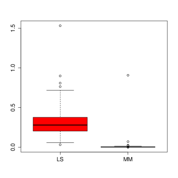
Lemma A.3.

Assume that ρ𝜌\rho satisfies C2 and let 𝒱=[σ1,σ2]𝒱subscript𝜎1subscript𝜎2{\mathcal{V}}=[\sigma_{1},\sigma_{2}] with 0<σ1<σ20subscript𝜎1subscript𝜎20<\sigma_{1}<\sigma_{2} some neighbourhood of the errors scale σ𝜎\sigma. Then, the function L(a,𝐛,g1,,gp,ς)𝐿𝑎𝐛subscript𝑔1subscript𝑔𝑝𝜍L\left(a,\mathbf{b},g_{1},\dots,g_{p},\varsigma\right) satisfies the following equicontinuity condition: for any ν>0𝜈0\nu>0 there exists δ>0𝛿0\delta>0 such that for any ς1,ς2𝒱subscript𝜍1subscript𝜍2𝒱\varsigma_{1},\varsigma_{2}\in{\mathcal{V}},

|ς1ς2|<δsupa,𝐛qg1𝒮1,,gp𝒮p|L(a,𝐛,g1,,gp,ς1)L(a,𝐛,g1,,gp,ς2)|<ν.subscript𝜍1subscript𝜍2𝛿subscriptsubscriptsupremumformulae-sequence𝑎𝐛superscript𝑞formulae-sequencesubscript𝑔1subscript𝒮1subscript𝑔𝑝subscript𝒮𝑝𝐿𝑎𝐛subscript𝑔1subscript𝑔𝑝subscript𝜍1𝐿𝑎𝐛subscript𝑔1subscript𝑔𝑝subscript𝜍2𝜈|\varsigma_{1}-\varsigma_{2}|<\delta\Rightarrow\mathop{\sup_{a\in\mathbb{R},\mathbf{b}\in\mathbb{R}^{q}}}_{g_{1}\in{\mathcal{S}}_{1},\dots,g_{p}\in{\mathcal{S}}_{p}}|L(a,\mathbf{b},g_{1},\dots,g_{p},\varsigma_{1})-L(a,\mathbf{b},g_{1},\dots,g_{p},\varsigma_{2})|<\nu\,.

Proof. Let ν>0𝜈0\nu>0 and a𝑎a\in\mathbb{R}, 𝐛q𝐛superscript𝑞\mathbf{b}\in\mathbb{R}^{q} and gj(x)=s=1kj1cs(j)Bs(j)(x)𝒮jsubscript𝑔𝑗𝑥superscriptsubscript𝑠1subscript𝑘𝑗1superscriptsubscript𝑐𝑠𝑗superscriptsubscript𝐵𝑠𝑗𝑥subscript𝒮𝑗g_{j}(x)=\sum_{s=1}^{k_{j}-1}c_{s}^{(j)}B_{s}^{(j)}(x)\in{\mathcal{S}}_{j}, 1jp1𝑗𝑝1\leq j\leq p. Using a Taylor expansion of order one and taking into account that ρ=ψsuperscript𝜌𝜓\rho^{\prime}=\psi, we have that

L(a,𝐛,g1,,gp,ς1)L(a,𝐛,g1,,gp,ς2)𝐿𝑎𝐛subscript𝑔1subscript𝑔𝑝subscript𝜍1𝐿𝑎𝐛subscript𝑔1subscript𝑔𝑝subscript𝜍2\displaystyle L(a,\mathbf{b},g_{1},\dots,g_{p},\varsigma_{1})-L(a,\mathbf{b},g_{1},\dots,g_{p},\varsigma_{2})
=𝔼[ψ(Y1a𝐛t𝐙j=1pgj(Xj)ξ)Y1a𝐛t𝐙j=1pgj(Xj)ξ2(ς2ς1)]absent𝔼delimited-[]𝜓subscript𝑌1𝑎superscript𝐛t𝐙superscriptsubscript𝑗1𝑝subscript𝑔𝑗subscript𝑋𝑗𝜉subscript𝑌1𝑎superscript𝐛t𝐙superscriptsubscript𝑗1𝑝subscript𝑔𝑗subscript𝑋𝑗superscript𝜉2subscript𝜍2subscript𝜍1\displaystyle=\mathbb{E}\left[\psi\left(\frac{Y_{1}-a-\mathbf{b}^{\mbox{\footnotesize\sc t}}\mathbf{Z}-\sum_{j=1}^{p}g_{j}(X_{j})}{\xi}\right)\,\frac{Y_{1}-a-\mathbf{b}^{\mbox{\footnotesize\sc t}}\mathbf{Z}-\sum_{j=1}^{p}g_{j}(X_{j})}{\xi^{2}}(\varsigma_{2}-\varsigma_{1})\right]

where ξ𝜉\xi is an intermediate point between ς1subscript𝜍1\varsigma_{1} and ς2subscript𝜍2\varsigma_{2}, so ξσ1>0𝜉subscript𝜎10\xi\geq\sigma_{1}>0. Using that ζ(s)=sψ(s)𝜁𝑠𝑠𝜓𝑠\zeta(s)=s\psi(s) is bounded, we get the bound

|L(a,𝐛,g1,,gp,ς1)L(a,𝐛,g1,,gp,ς2)|ζσ1|ς2ς1|.𝐿𝑎𝐛subscript𝑔1subscript𝑔𝑝subscript𝜍1𝐿𝑎𝐛subscript𝑔1subscript𝑔𝑝subscript𝜍2subscriptnorm𝜁subscript𝜎1subscript𝜍2subscript𝜍1|L(a,\mathbf{b},g_{1},\dots,g_{p},\varsigma_{1})-L(a,\mathbf{b},g_{1},\dots,g_{p},\varsigma_{2})|\leq\frac{\|\zeta\|_{\infty}}{\sigma_{1}}|\varsigma_{2}-\varsigma_{1}|\,.

Finally, by taking δ=σ1ν/(2ζ)𝛿subscript𝜎1𝜈2𝜁\delta=\sigma_{1}\nu/(2\zeta) and noting that the bound does not depend on a,𝐛,g1,,gp𝑎𝐛subscript𝑔1subscript𝑔𝑝a,\mathbf{b},g_{1},\dots,g_{p}, the result follows.  ∎

In order to prove Theorem 3.3 and Proposition 3.4, we introduce some additional notation. The unit ball in rsubscript𝑟{\mathcal{H}}_{r} will be denoted as 𝒱1(r)={ηr:ηr1}superscriptsubscript𝒱1𝑟conditional-set𝜂subscript𝑟subscriptnorm𝜂subscript𝑟1{\mathcal{V}}_{1}^{(r)}=\left\{\eta\in{\mathcal{H}}_{r}\,:\,\|\eta\|_{{\mathcal{H}}_{r}}\leq 1\right\}. Besides, denote q={𝐛q:𝐛1}subscript𝑞conditional-set𝐛superscript𝑞norm𝐛1{\mathcal{B}}_{q}=\{\mathbf{b}\in\mathbb{R}^{q}\,:\,\|\mathbf{b}\|\leq 1\} the unit ball in qsuperscript𝑞\mathbb{R}^{q}. The following result is needed to derive Theorem 3.3.

Lemma A.4.

Assume that ρ𝜌\rho satisfies C2 and that L(μ,𝛃,η1,,ηp,σ)=bρ<1𝐿𝜇𝛃subscript𝜂1subscript𝜂𝑝𝜎subscript𝑏𝜌1L(\mu,\mbox{\boldmath$\beta$},\eta_{1},\dots,\eta_{p},\sigma)=b_{\rho}<1. Let (μ^,𝛃^,η^1,,η^p)×q×𝒮1××𝒮p^𝜇^𝛃subscript^𝜂1subscript^𝜂𝑝superscript𝑞subscript𝒮1subscript𝒮𝑝(\widehat{\mu},\widehat{\mbox{\boldmath$\beta$}},\widehat{\eta}_{1},\dots,\widehat{\eta}_{p})\in\mathbb{R}\times\mathbb{R}^{q}\times{\mathcal{S}}_{1}\times\dots\times{\mathcal{S}}_{p} be such that L(μ^,𝛃^,η^1,,η^p,σ)a.s.L(μ,𝛃,η1,,ηp,σ)L(\widehat{\mu},\widehat{\mbox{\boldmath$\beta$}},\widehat{\eta}_{1},\dots,\widehat{\eta}_{p},\sigma)\buildrel a.s.\over{\longrightarrow}L(\mu,\mbox{\boldmath$\beta$},\eta_{1},\dots,\eta_{p},\sigma). Assume that 𝔼𝐙2<𝔼superscriptnorm𝐙2\mathbb{E}\|\mathbf{Z}\|^{2}<\infty and that C3 and C7 hold with c<1bρ𝑐1subscript𝑏𝜌c<1-b_{\rho}. Then, we have that there exists M𝑀M such that

(mnm{|μ^μ|+𝜷^𝜷+j=1pη^jηjjM})=1subscript𝑚subscript𝑛𝑚^𝜇𝜇norm^𝜷𝜷superscriptsubscript𝑗1𝑝subscriptnormsubscript^𝜂𝑗subscript𝜂𝑗subscript𝑗𝑀1\mathbb{P}\left(\bigcup_{m\in\mathbb{N}}\bigcap_{n\geq m}\left\{|\widehat{\mu}-\mu|+\|\widehat{\mbox{\boldmath$\beta$}}-\mbox{\boldmath$\beta$}\|+\sum_{j=1}^{p}{\|\widehat{\eta}_{j}-\eta_{j}}\|_{{\mathcal{H}}_{j}}\leq M\right\}\right)=1

Proof. Given δ>0𝛿0\delta>0, let Cδsubscript𝐶𝛿C_{\delta} be such for for any CCδ𝐶subscript𝐶𝛿C\geq C_{\delta}

(𝐙C)<δ.norm𝐙𝐶𝛿\mathbb{P}(\|\mathbf{Z}\|\geq C)<\delta\,. (A.8)

Fix 𝐭=(a,𝐛,g1,,gp)={(a,𝐛,g1,,gp)×q×C([0,1])××C([0,1]):|a|+𝐛+j=1pgj=1}[1,1]×q×𝒱1(r1)××𝒱1(1)𝐭𝑎𝐛subscript𝑔1subscript𝑔𝑝conditional-setsuperscript𝑎superscript𝐛superscriptsubscript𝑔1superscriptsubscript𝑔𝑝superscript𝑞𝐶01𝐶01superscript𝑎normsuperscript𝐛superscriptsubscript𝑗1𝑝subscriptnormsuperscriptsubscript𝑔𝑗111subscript𝑞superscriptsubscript𝒱1subscript𝑟1superscriptsubscript𝒱11\mathbf{t}=(a,\mathbf{b},g_{1},\dots,g_{p})\in{\mathcal{B}}=\{(a^{*},\mathbf{b}^{*},g_{1}^{*},\dots,g_{p}^{*})\in\mathbb{R}\times\mathbb{R}^{q}\times C([0,1])\times\dots\times C([0,1])\,:|a^{*}|+\|\mathbf{b}^{*}\|+\sum_{j=1}^{p}\|g_{j}^{*}\|_{\infty}=1\}[-1,1]\times{\mathcal{B}}_{q}\times{\mathcal{V}}_{1}^{(r_{1})}\times\dots\times{\mathcal{V}}_{1}^{(1)}. Assumption C7 allows to select a positive real number ϕ𝐭subscriptitalic-ϕ𝐭\phi_{\mathbf{t}} such that ϕ𝐭subscriptitalic-ϕ𝐭\phi_{\mathbf{t}} is a continuity point of |a+𝐛t𝐙+j=1pgj(Xj)|𝑎superscript𝐛t𝐙superscriptsubscript𝑗1𝑝subscript𝑔𝑗subscript𝑋𝑗\left|a+\mathbf{b}^{\mbox{\footnotesize\sc t}}\mathbf{Z}+\sum_{j=1}^{p}g_{j}(X_{j})\right| and

(|a+𝐛t𝐙+j=1pgj(Xj)|<ϕ𝐭)<c.𝑎superscript𝐛t𝐙superscriptsubscript𝑗1𝑝subscript𝑔𝑗subscript𝑋𝑗subscriptitalic-ϕ𝐭𝑐\mathbb{P}\left(\left|a+\mathbf{b}^{\mbox{\footnotesize\sc t}}\mathbf{Z}+\sum_{j=1}^{p}g_{j}(X_{j})\right|<\phi_{\mathbf{t}}\right)<c\,. (A.9)

Denote ϑ𝐭=ϕ𝐭/2subscriptitalic-ϑ𝐭subscriptitalic-ϕ𝐭2\vartheta_{\mathbf{t}}=\phi_{\mathbf{t}}/2 and v𝐭=ϕ𝐭/(2(C+p+1))subscript𝑣𝐭subscriptitalic-ϕ𝐭2𝐶𝑝1v_{\mathbf{t}}=\phi_{\mathbf{t}}/(2(C+p+1)). Then, if asuperscript𝑎a^{*}\in\mathbb{R}, 𝐛qsuperscript𝐛superscript𝑞\mathbf{b}^{*}\in\mathbb{R}^{q} and g1,,gpC([0,1])subscriptsuperscript𝑔1superscriptsubscript𝑔𝑝𝐶01g^{*}_{1},\dots,g_{p}^{*}\in C([0,1]) are such that |aa|+𝐛𝐛+max1jp{gjgj}<v𝐭𝑎superscript𝑎normsuperscript𝐛𝐛subscript1𝑗𝑝subscriptnormsuperscriptsubscript𝑔𝑗subscript𝑔𝑗subscript𝑣𝐭|a-a^{*}|+\|\mathbf{b}^{*}-\mathbf{b}\|+\max_{1\leq j\leq p}\{\|g_{j}^{*}-g_{j}\|_{\infty}\}<v_{\mathbf{t}}, we have that

(|a+𝐙t𝐛+j=1pgj(Xj)|ϑ𝐭)superscript𝑎superscript𝐙tsuperscript𝐛superscriptsubscript𝑗1𝑝superscriptsubscript𝑔𝑗subscript𝑋𝑗subscriptitalic-ϑ𝐭\displaystyle\mathbb{P}\left(\left|a^{*}+\mathbf{Z}^{\mbox{\footnotesize\sc t}}\mathbf{b}^{*}+\sum_{j=1}^{p}g_{j}^{*}(X_{j})\right|\geq\vartheta_{\mathbf{t}}\right) (|a+𝐛t𝐙+j=1pgj(Xj)|ϕ𝐭)absent𝑎superscript𝐛t𝐙superscriptsubscript𝑗1𝑝subscript𝑔𝑗subscript𝑋𝑗subscriptitalic-ϕ𝐭\displaystyle\geq\mathbb{P}\left(\left|a+\mathbf{b}^{\mbox{\footnotesize\sc t}}\mathbf{Z}+\sum_{j=1}^{p}g_{j}(X_{j})\right|\geq\phi_{\mathbf{t}}\right)
(|aa|+𝐛𝐛𝐙+|j=1p(gjgj)(Xj)|ϑ𝐭)𝑎superscript𝑎normsuperscript𝐛𝐛norm𝐙superscriptsubscript𝑗1𝑝superscriptsubscript𝑔𝑗subscript𝑔𝑗subscript𝑋𝑗subscriptitalic-ϑ𝐭\displaystyle-\mathbb{P}\left(|a-a^{*}|+\|\mathbf{b}^{*}-\mathbf{b}\|\|\mathbf{Z}\|+\left|\sum_{j=1}^{p}(g_{j}^{*}-g_{j})(X_{j})\right|\geq\vartheta_{\mathbf{t}}\right)
(|a+𝐛t𝐙+j=1pgj(Xj)|ϕ𝐭)(v𝐭(p+1+𝐙)ϑ𝐭)=A(𝐭)absent𝑎superscript𝐛t𝐙superscriptsubscript𝑗1𝑝subscript𝑔𝑗subscript𝑋𝑗subscriptitalic-ϕ𝐭subscript𝑣𝐭𝑝1norm𝐙subscriptitalic-ϑ𝐭𝐴𝐭\displaystyle\geq\mathbb{P}\left(\left|a+\mathbf{b}^{\mbox{\footnotesize\sc t}}\mathbf{Z}+\sum_{j=1}^{p}g_{j}(X_{j})\right|\geq\phi_{\mathbf{t}}\right)-\mathbb{P}\left(v_{\mathbf{t}}(p+1+\|\mathbf{Z}\|)\geq\vartheta_{\mathbf{t}}\right)=A(\mathbf{t})

Hence, noting that (A.9) and (A.8) imply that A(𝐭)>1cδ𝐴𝐭1𝑐𝛿A(\mathbf{t})>1-c-\delta, we conclude that

inf|aa|+𝐛𝐛+max1jp{gjgj}<v𝐭(|a+𝐙t𝐛+j=1pgj(Xj)|ϑ𝐭)1cδ.subscriptinfimum𝑎superscript𝑎normsuperscript𝐛𝐛subscript1𝑗𝑝subscriptnormsuperscriptsubscript𝑔𝑗subscript𝑔𝑗subscript𝑣𝐭superscript𝑎superscript𝐙tsuperscript𝐛superscriptsubscript𝑗1𝑝superscriptsubscript𝑔𝑗subscript𝑋𝑗subscriptitalic-ϑ𝐭1𝑐𝛿\inf_{|a-a^{*}|+\|\mathbf{b}^{*}-\mathbf{b}\|+\max_{1\leq j\leq p}\{\|g_{j}^{*}-g_{j}\|_{\infty}\}<v_{\mathbf{t}}}\mathbb{P}\left(\left|a^{*}+\mathbf{Z}^{\mbox{\footnotesize\sc t}}\mathbf{b}^{*}+\sum_{j=1}^{p}g_{j}^{*}(X_{j})\right|\geq\vartheta_{\mathbf{t}}\right)\geq 1-c-\delta\,. (A.10)

Let us considering the covering of {\mathcal{B}} given by {B(𝐭,v𝐭)}𝐭subscript𝐵𝐭subscript𝑣𝐭𝐭\{B(\mathbf{t},v_{\mathbf{t}})\}_{\mathbf{t}\in{\mathcal{B}}}, where B(𝐭,ν)𝐵𝐭𝜈B(\mathbf{t},\nu) is defined as

B(𝐭,ν)={(a,𝐛,g1,,gp)×q×C([0,1])××C([0,1]):|aa|+𝐛𝐛+max1jp{gjgj}<ν}.𝐵𝐭𝜈conditional-setsuperscript𝑎superscript𝐛superscriptsubscript𝑔1superscriptsubscript𝑔𝑝superscript𝑞𝐶01𝐶01𝑎superscript𝑎normsuperscript𝐛𝐛subscript1𝑗𝑝subscriptnormsuperscriptsubscript𝑔𝑗subscript𝑔𝑗𝜈B(\mathbf{t},\nu)=\left\{(a^{*},\mathbf{b}^{*},g_{1}^{*},\dots,g_{p}^{*})\in\mathbb{R}\times\mathbb{R}^{q}\times C([0,1])\times\dots\times C([0,1])\,:\,|a-a^{*}|+\|\mathbf{b}^{*}-\mathbf{b}\|+\max_{1\leq j\leq p}\{\|g_{j}^{*}-g_{j}\|_{\infty}\}<\nu\right\}\,.

The fact that 𝒱1(1)××𝒱1(1)superscriptsubscript𝒱11superscriptsubscript𝒱11{\mathcal{V}}_{1}^{(1)}\times\dots\times{\mathcal{V}}_{1}^{(1)} is a compact set in C([0,1])××C([0,1])𝐶01𝐶01C([0,1])\times\dots\times C([0,1]) entails that there exists 𝐭=(a,𝐛,g1,,,gp,)subscript𝐭subscript𝑎subscript𝐛subscript𝑔1subscript𝑔𝑝\mathbf{t}_{\ell}=(a_{\ell},\mathbf{b}_{\ell},g_{1,\ell},\dots,g_{p,\ell})\in{\mathcal{B}}, for 1s1𝑠1\leq\ell\leq s, such that =1sB(𝐭,v)superscriptsubscript1𝑠𝐵subscript𝐭subscript𝑣{\mathcal{B}}\subset\bigcup_{\ell=1}^{s}B(\mathbf{t}_{\ell},v_{\ell}) where we have denoted v=v𝐭subscript𝑣subscript𝑣subscript𝐭v_{\ell}=v_{\mathbf{t}_{\ell}}. Therefore, from A.10 we obtain that

min1sinf|aa|+𝐛𝐛+max{gjgj,}<v(|a+𝐛t𝐙+j=1pgj(Xj)|>ϑ)>1cδ,subscript1𝑠subscriptinfimum𝑎subscript𝑎norm𝐛subscript𝐛subscriptnormsubscript𝑔𝑗subscript𝑔𝑗subscript𝑣𝑎superscript𝐛t𝐙superscriptsubscript𝑗1𝑝subscript𝑔𝑗subscript𝑋𝑗subscriptitalic-ϑ1𝑐𝛿\min_{1\leq\ell\leq s}\,\,\inf_{|a-a_{\ell}|+\|\mathbf{b}-\mathbf{b}_{\ell}\|+\max\{\|g_{j}-g_{j,\ell}\|_{\infty}\}<v_{\ell}}\mathbb{P}\left(\left|a+\mathbf{b}^{\mbox{\footnotesize\sc t}}\mathbf{Z}+\sum_{j=1}^{p}g_{j}(X_{j})\right|>\vartheta_{\ell}\right)>1-c-\delta\,,

where ϑ=ϑ𝐭subscriptitalic-ϑsubscriptitalic-ϑsubscript𝐭\vartheta_{\ell}=\vartheta_{\mathbf{t}_{\ell}}. Henceforth, for any 𝐭=(a,𝐛,g1,,gp)𝐭𝑎𝐛subscript𝑔1subscript𝑔𝑝\mathbf{t}=(a,\mathbf{b},g_{1},\dots,g_{p})\in{\mathcal{B}}, there exists 1s1𝑠1\leq\ell\leq s such that

(|a+𝐛t𝐙+j=1pgj(Xj)|>ϑ)>1cδ.𝑎superscript𝐛t𝐙superscriptsubscript𝑗1𝑝subscript𝑔𝑗subscript𝑋𝑗subscriptitalic-ϑ1𝑐𝛿\mathbb{P}\left(\left|a+\mathbf{b}^{\mbox{\footnotesize\sc t}}\mathbf{Z}+\sum_{j=1}^{p}g_{j}(X_{j})\right|>\vartheta_{\ell}\right)>1-c-\delta\,. (A.11)

Let 𝒩𝒩{\mathcal{N}} be such that (𝒩)=0𝒩0\mathbb{P}({\mathcal{N}})=0 and for each ω𝒩𝜔𝒩\omega\notin{\mathcal{N}}, L(μ^,𝜷^,η^1,,η^p,σ)L(μ,𝜷,η1,,ηp,σ)=bρ𝐿^𝜇^𝜷subscript^𝜂1subscript^𝜂𝑝𝜎𝐿𝜇𝜷subscript𝜂1subscript𝜂𝑝𝜎subscript𝑏𝜌L(\widehat{\mu},\widehat{\mbox{\boldmath$\beta$}},\widehat{\eta}_{1},\dots,\widehat{\eta}_{p},\sigma)\to L(\mu,\mbox{\boldmath$\beta$},\eta_{1},\dots,\eta_{p},\sigma)=b_{\rho}. Fix ω𝒩𝜔𝒩\omega\notin{\mathcal{N}} and let ξ>0𝜉0\xi>0 such that bρ+ξ<1csubscript𝑏𝜌𝜉1𝑐b_{\rho}+\xi<1-c. Then, there exists n0subscript𝑛0n_{0}\in\mathbb{N} such that for all nn0𝑛subscript𝑛0n\geq n_{0}, L(μ^,𝜷^,η^1,,η^p,σ)bρ+ξ/2𝐿^𝜇^𝜷subscript^𝜂1subscript^𝜂𝑝𝜎subscript𝑏𝜌𝜉2L(\widehat{\mu},\widehat{\mbox{\boldmath$\beta$}},\widehat{\eta}_{1},\dots,\widehat{\eta}_{p},\sigma)\leq b_{\rho}+\xi/2.

We want to show that there exists M>0𝑀0M>0 such that, for ω𝒩𝜔𝒩\omega\notin{\mathcal{N}}, lim supn{|μ^μ|+𝜷^𝜷+\limsup_{n\to\infty}\left\{|\widehat{\mu}-\mu|+\|\widehat{\mbox{\boldmath$\beta$}}-\mbox{\boldmath$\beta$}\|+\right. j=1pη^jηj1}M\left.\sum_{j=1}^{p}\|\widehat{\eta}_{j}-\eta_{j}\|_{{\mathcal{H}}_{1}}\right\}\leq M. For that purpose, it will be enough to show that there exists M>0𝑀0M>0 such that

inf|aμ|+𝐛𝜷+j=1pgjηj1>ML(a,𝐛,g1,,gp)bρ+ξ.subscriptinfimum𝑎𝜇norm𝐛𝜷superscriptsubscript𝑗1𝑝subscriptnormsubscript𝑔𝑗subscript𝜂𝑗subscript1𝑀𝐿𝑎𝐛subscript𝑔1subscript𝑔𝑝subscript𝑏𝜌𝜉\inf_{|a-\mu|+\|\mathbf{b}-{\mbox{\scriptsize${\mbox{\boldmath$\beta$}}$}}\|+\sum_{j=1}^{p}\|g_{j}-\eta_{j}\|_{{\mathcal{H}}_{1}}>M}L(a,\mathbf{b},g_{1},\dots,g_{p})\geq b_{\rho}+\xi\,.

Denote as R(u)=𝔼ρ(εu/σ)𝑅𝑢𝔼𝜌𝜀𝑢𝜎R(u)=\mathbb{E}\rho\left(\varepsilon-u/\sigma\right). First note that the independence between the errors and the covariates entails that

L(a,𝐛,g1,,gp,σ)𝐿𝑎𝐛subscript𝑔1subscript𝑔𝑝𝜎\displaystyle L(a,\mathbf{b},g_{1},\dots,g_{p},\sigma) =\displaystyle= 𝔼ρ(ε+μa+(𝜷𝐛)t𝐙+j=1p(ηjgj)(Xj)σ)𝔼𝜌𝜀𝜇𝑎superscript𝜷𝐛t𝐙superscriptsubscript𝑗1𝑝subscript𝜂𝑗subscript𝑔𝑗subscript𝑋𝑗𝜎\displaystyle\mathbb{E}\rho\left(\varepsilon+\frac{\mu-a+(\mbox{\boldmath$\beta$}-\mathbf{b})^{\mbox{\footnotesize\sc t}}\mathbf{Z}+\sum_{j=1}^{p}(\eta_{j}-g_{j})(X_{j})}{\sigma}\right)
=\displaystyle= 𝔼R(aμ+(𝐛𝜷)t𝐙+j=1p(gjηj)(Xj)).𝔼𝑅𝑎𝜇superscript𝐛𝜷t𝐙superscriptsubscript𝑗1𝑝subscript𝑔𝑗subscript𝜂𝑗subscript𝑋𝑗\displaystyle\mathbb{E}R\left(a-\mu+(\mathbf{b}-\mbox{\boldmath$\beta$})^{\mbox{\footnotesize\sc t}}\mathbf{Z}+\sum_{j=1}^{p}(g_{j}-\eta_{j})(X_{j})\right)\,.

Using that lim|u|+R(u)=1subscript𝑢𝑅𝑢1\lim_{|u|\to+\infty}R(u)=1, we get that for any δ>0𝛿0\delta>0, there exists u0subscript𝑢0u_{0} such that |u|u0𝑢subscript𝑢0|u|\geq u_{0},

R(u)>1δ.𝑅𝑢1𝛿R(u)>1-\delta\,. (A.12)

Choose M>u0/(min1sϑ)𝑀subscript𝑢0subscript1𝑠subscriptitalic-ϑM>u_{0}/(\min_{1\leq\ell\leq s}\vartheta_{\ell}) and let (ak,𝐛k,g1,k,,gp,k)×q×1××1subscript𝑎𝑘subscript𝐛𝑘subscript𝑔1𝑘subscript𝑔𝑝𝑘superscript𝑞subscript1subscript1(a_{k},\mathbf{b}_{k},g_{1,k},\dots,g_{p,k})\in\mathbb{R}\times\mathbb{R}^{q}\times{\mathcal{H}}_{1}\times\dots\times{\mathcal{H}}_{1} such that νk=|akμ|+𝐛k𝜷+j=1pgj,kηj1>Msubscript𝜈𝑘subscript𝑎𝑘𝜇normsubscript𝐛𝑘𝜷superscriptsubscript𝑗1𝑝subscriptnormsubscript𝑔𝑗𝑘subscript𝜂𝑗subscript1𝑀\nu_{k}=|a_{k}-\mu|+\|\mathbf{b}_{k}-\mbox{\boldmath$\beta$}\|+\sum_{j=1}^{p}\|g_{j,k}-\eta_{j}\|_{{\mathcal{H}}_{1}}>M and

L(ak,𝐛k,g1,k,,gp,k,σ)inf|aμ|+𝐛𝜷+j=1pgjηj1>ML(a,𝐛,g1,,gp,σ).𝐿subscript𝑎𝑘subscript𝐛𝑘subscript𝑔1𝑘subscript𝑔𝑝𝑘𝜎subscriptinfimum𝑎𝜇norm𝐛𝜷superscriptsubscript𝑗1𝑝subscriptnormsubscript𝑔𝑗subscript𝜂𝑗subscript1𝑀𝐿𝑎𝐛subscript𝑔1subscript𝑔𝑝𝜎L(a_{k},\mathbf{b}_{k},g_{1,k},\dots,g_{p,k},\sigma)\to\inf_{|a-\mu|+\|\mathbf{b}-\mbox{\scriptsize${\mbox{\boldmath$\beta$}}$}\|+\sum_{j=1}^{p}\|g_{j}-\eta_{j}\|_{{\mathcal{H}}_{1}}>M}L(a,\mathbf{b},g_{1},\dots,g_{p},\sigma)\,.

Denote as a~k=(akμ)/νksubscript~𝑎𝑘subscript𝑎𝑘𝜇subscript𝜈𝑘\widetilde{a}_{k}=(a_{k}-\mu)/\nu_{k}, 𝐛~k=(𝐛k𝜷)/νksubscript~𝐛𝑘subscript𝐛𝑘𝜷subscript𝜈𝑘\widetilde{\mathbf{b}}_{k}=(\mathbf{b}_{k}-\mbox{\boldmath$\beta$})/\nu_{k} and g~j,k=(gj,kηj)/νksubscript~𝑔𝑗𝑘subscript𝑔𝑗𝑘subscript𝜂𝑗subscript𝜈𝑘\widetilde{g}_{j,k}=(g_{j,k}-\eta_{j})/\nu_{k}, for 1jp1𝑗𝑝1\leq j\leq p. Then (a~k,𝐛~k,g~1,k,,g~p,k)subscript~𝑎𝑘subscript~𝐛𝑘subscript~𝑔1𝑘subscript~𝑔𝑝𝑘(\widetilde{a}_{k},\widetilde{\mathbf{b}}_{k},\widetilde{g}_{1,k},\dots,\widetilde{g}_{p,k})\in{\mathcal{B}}. Thus, using A.11 we obtain that there exists 1=(k)s1𝑘𝑠1\leq\ell=\ell(k)\leq s such that

(|a~k+𝐛~kt𝐙+j=1pg~j,k(Xj)|>ϑ)>1cδ.subscript~𝑎𝑘superscriptsubscript~𝐛𝑘t𝐙superscriptsubscript𝑗1𝑝subscript~𝑔𝑗𝑘subscript𝑋𝑗subscriptitalic-ϑ1𝑐𝛿\mathbb{P}\left(\left|\widetilde{a}_{k}+\widetilde{\mathbf{b}}_{k}^{\mbox{\footnotesize\sc t}}\mathbf{Z}+\sum_{j=1}^{p}\widetilde{g}_{j,k}(X_{j})\right|>\vartheta_{\ell}\right)>1-c-\delta\,. (A.13)

Using that νk>M>u0/ϑsubscript𝜈𝑘𝑀subscript𝑢0subscriptitalic-ϑ\nu_{k}>M>u_{0}/\vartheta_{\ell} and denoting uk(𝐙,𝐗)=νk(a~k+𝐛~kt𝐙+j=1pg~j,k(Xj))subscript𝑢𝑘𝐙𝐗subscript𝜈𝑘subscript~𝑎𝑘superscriptsubscript~𝐛𝑘t𝐙superscriptsubscript𝑗1𝑝subscript~𝑔𝑗𝑘subscript𝑋𝑗u_{k}(\mathbf{Z},\mathbf{X})=\nu_{k}\left(\widetilde{a}_{k}+\widetilde{\mathbf{b}}_{k}^{\mbox{\footnotesize\sc t}}\mathbf{Z}+\sum_{j=1}^{p}\widetilde{g}_{j,k}(X_{j})\right), we obtain that |uk(𝐙,𝐗)|>u0subscript𝑢𝑘𝐙𝐗subscript𝑢0|u_{k}(\mathbf{Z},\mathbf{X})|>u_{0} whenever |a~k+𝐛~kt𝐙+j=1pg~j,k(Xj)|>ϑsubscript~𝑎𝑘superscriptsubscript~𝐛𝑘t𝐙superscriptsubscript𝑗1𝑝subscript~𝑔𝑗𝑘subscript𝑋𝑗subscriptitalic-ϑ\left|\widetilde{a}_{k}+\widetilde{\mathbf{b}}_{k}^{\mbox{\footnotesize\sc t}}\mathbf{Z}+\sum_{j=1}^{p}\widetilde{g}_{j,k}(X_{j})\right|>\vartheta_{\ell}, which together with A.12 leads to

L(ak,𝐛k,g1,k,,g~p,k,σ)𝐿subscript𝑎𝑘subscript𝐛𝑘subscript𝑔1𝑘subscript~𝑔𝑝𝑘𝜎\displaystyle L(a_{k},\mathbf{b}_{k},g_{1,k},\dots,\widetilde{g}_{p,k},\sigma) =\displaystyle= 𝔼R(akμ+(𝐛k𝜷)t𝐙+j=1p(gj,kηj)(Xj))𝔼𝑅subscript𝑎𝑘𝜇superscriptsubscript𝐛𝑘𝜷t𝐙superscriptsubscript𝑗1𝑝subscript𝑔𝑗𝑘subscript𝜂𝑗subscript𝑋𝑗\displaystyle\mathbb{E}R\left(a_{k}-\mu+(\mathbf{b}_{k}-\mbox{\boldmath$\beta$})^{\mbox{\footnotesize\sc t}}\mathbf{Z}+\sum_{j=1}^{p}(g_{j,k}-\eta_{j})(X_{j})\right)
=\displaystyle= 𝔼R(uk(𝐙,𝐗))𝔼𝑅subscript𝑢𝑘𝐙𝐗\displaystyle\mathbb{E}R(u_{k}(\mathbf{Z},\mathbf{X}))
\displaystyle\geq 𝔼R(uk(𝐙,𝐗))𝕀|a~k+𝐛~kt𝐙+j=1pg~j,k(Xj)|>ϑ𝔼𝑅subscript𝑢𝑘𝐙𝐗subscript𝕀subscript~𝑎𝑘superscriptsubscript~𝐛𝑘t𝐙superscriptsubscript𝑗1𝑝subscript~𝑔𝑗𝑘subscript𝑋𝑗subscriptitalic-ϑ\displaystyle\mathbb{E}R(u_{k}(\mathbf{Z},\mathbf{X}))\mathbb{I}_{|\widetilde{a}_{k}+\widetilde{\mathbf{b}}_{k}^{\mbox{\footnotesize\sc t}}\mathbf{Z}+\sum_{j=1}^{p}\widetilde{g}_{j,k}(X_{j})|>\vartheta_{\ell}}
>\displaystyle> (1δ)(|a~k+𝐛~kt𝐙+j=1pg~j,k(Xj)|>ϑ)1𝛿subscript~𝑎𝑘superscriptsubscript~𝐛𝑘t𝐙superscriptsubscript𝑗1𝑝subscript~𝑔𝑗𝑘subscript𝑋𝑗subscriptitalic-ϑ\displaystyle(1-\delta)\,\mathbb{P}\left(\left|\widetilde{a}_{k}+\widetilde{\mathbf{b}}_{k}^{\mbox{\footnotesize\sc t}}\mathbf{Z}+\sum_{j=1}^{p}\widetilde{g}_{j,k}(X_{j})\right|>\vartheta_{\ell}\right)
>\displaystyle> (1δ)(1cδ),1𝛿1𝑐𝛿\displaystyle(1-\delta)(1-c-\delta)\,,

where the last inequality follows from A.13. Therefore,

inf|aμ|+𝐛𝜷+j=1pgjηj1>ML(a,𝐛,g1,,gp,σ)(1δ)(1cδ).subscriptinfimum𝑎𝜇norm𝐛𝜷superscriptsubscript𝑗1𝑝subscriptnormsubscript𝑔𝑗subscript𝜂𝑗subscript1𝑀𝐿𝑎𝐛subscript𝑔1subscript𝑔𝑝𝜎1𝛿1𝑐𝛿\inf_{|a-\mu|+\|\mathbf{b}-\mbox{\scriptsize${\mbox{\boldmath$\beta$}}$}\|+\sum_{j=1}^{p}\|g_{j}-\eta_{j}\|_{{\mathcal{H}}_{1}}>M}L(a,\mathbf{b},g_{1},\dots,g_{p},\sigma)\geq(1-\delta)(1-c-\delta)\,.

The proof follows now easily noting that limδ0(1δ)(1cδ)=1c>bρ+ξsubscript𝛿01𝛿1𝑐𝛿1𝑐subscript𝑏𝜌𝜉\lim_{\delta\to 0}(1-\delta)(1-c-\delta)=1-c>b_{\rho}+\xi, so we can choose δ𝛿\delta and consequently M𝑀M such that

inf|aμ|+𝐛𝜷+j=1pgjηj1>ML(a,𝐛,g1,,gp,σ)>bρ+ξ>L(μ^,𝜷^,η^1,,η^p,σ)subscriptinfimum𝑎𝜇norm𝐛𝜷superscriptsubscript𝑗1𝑝subscriptnormsubscript𝑔𝑗subscript𝜂𝑗subscript1𝑀𝐿𝑎𝐛subscript𝑔1subscript𝑔𝑝𝜎subscript𝑏𝜌𝜉𝐿^𝜇^𝜷subscript^𝜂1subscript^𝜂𝑝𝜎\inf_{|a-\mu|+\|\mathbf{b}-\mbox{\scriptsize${\mbox{\boldmath$\beta$}}$}\|+\sum_{j=1}^{p}\|g_{j}-\eta_{j}\|_{{\mathcal{H}}_{1}}>M}L(a,\mathbf{b},g_{1},\dots,g_{p},\sigma)>b_{\rho}+\xi>L(\widehat{\mu},\widehat{\mbox{\boldmath$\beta$}},\widehat{\eta}_{1},\dots,\widehat{\eta}_{p},\sigma)

so |μ^μ|+𝜷^𝜷+j=1pη^jηj1M^𝜇𝜇norm^𝜷𝜷superscriptsubscript𝑗1𝑝subscriptnormsubscript^𝜂𝑗subscript𝜂𝑗subscript1𝑀|\widehat{\mu}-\mu|+\|\widehat{\mbox{\boldmath$\beta$}}-\mbox{\boldmath$\beta$}\|+\sum_{j=1}^{p}\|\widehat{\eta}_{j}-\eta_{j}\|_{{\mathcal{H}}_{1}}\leq M, concluding the proof. ∎
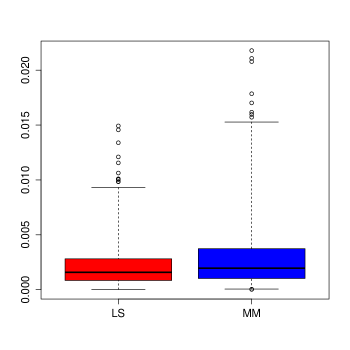
Proof of Theorem 3.3. Let Va,𝐛,g1,,gp,ς=ρ((ya𝐛t𝐳j=1pgj(xj))/ς)subscript𝑉𝑎𝐛subscript𝑔1subscript𝑔𝑝𝜍𝜌𝑦𝑎superscript𝐛t𝐳superscriptsubscript𝑗1𝑝subscript𝑔𝑗subscript𝑥𝑗𝜍V_{a,\mathbf{b},g_{1},\dots,g_{p},\varsigma}=\rho\left((y-a-\mathbf{b}^{\mbox{\footnotesize\sc t}}\mathbf{z}-\sum_{j=1}^{p}g_{j}(x_{j}))/\varsigma\right) and denote as P𝑃P the probability measure of (Y,𝐙t,𝐗t)tsuperscript𝑌superscript𝐙tsuperscript𝐗tt(Y,\mathbf{Z}^{\mbox{\footnotesize\sc t}},\mathbf{X}^{\mbox{\footnotesize\sc t}})^{\mbox{\footnotesize\sc t}} and as Pnsubscript𝑃𝑛P_{n} its corresponding empirical measure. Then, Ln(a,𝐛,g1,,gp,ς)=PnVa,𝐛,g1,,gp,ςsubscript𝐿𝑛𝑎𝐛subscript𝑔1subscript𝑔𝑝𝜍subscript𝑃𝑛subscript𝑉𝑎𝐛subscript𝑔1subscript𝑔𝑝𝜍L_{n}(a,\mathbf{b},g_{1},\dots,g_{p},\varsigma)=P_{n}V_{a,\mathbf{b},g_{1},\dots,g_{p},\varsigma} and L(a,𝐛,g1,,gp,ς)=PVa,𝐛,g1,,gp,ς𝐿𝑎𝐛subscript𝑔1subscript𝑔𝑝𝜍𝑃subscript𝑉𝑎𝐛subscript𝑔1subscript𝑔𝑝𝜍L(a,\mathbf{b},g_{1},\dots,g_{p},\varsigma)=PV_{a,\mathbf{b},g_{1},\dots,g_{p},\varsigma}.

The consistency of σ^^𝜎\widehat{\sigma} entails that given any neighbourhood 𝒱𝒱{\mathcal{V}} of σ𝜎\sigma, there exists a null set 𝒩𝒱subscript𝒩𝒱{\mathcal{N}}_{{\mathcal{V}}} such that for ω𝒩𝒱𝜔subscript𝒩𝒱\omega\notin{\mathcal{N}}_{{\mathcal{V}}}, there exists n0subscript𝑛0n_{0}\in\mathbb{N}, such that for all nn0𝑛subscript𝑛0n\geq n_{0} we have that σ^𝒱^𝜎𝒱\widehat{\sigma}\in{\mathcal{V}}.

Lemma A.2 implies that

An=supς>0,a,𝐛qg1𝒮1,,gp𝒮p|Ln(a,𝐛,g1,,gp,ς)L(a,𝐛,g1,,gp,ς)|a.s.0.A_{n}=\mathop{\sup_{\varsigma>0,a\in\mathbb{R},\mathbf{b}\in\mathbb{R}^{q}}}_{g_{1}\in{\mathcal{S}}_{1},\dots,g_{p}\in{\mathcal{S}}_{p}}|L_{n}(a,\mathbf{b},g_{1},\dots,g_{p},\varsigma)-L(a,\mathbf{b},g_{1},\dots,g_{p},\varsigma)|\buildrel a.s.\over{\longrightarrow}0\,. (A.14)

On the other hand, from Lemma 3.1 we have

L(μ,𝜷,η1,,ηp,σ)=mina,𝐛q,g1𝒢,,gp𝒢L(a,𝐛,g1,,gp,σ),𝐿𝜇𝜷subscript𝜂1subscript𝜂𝑝𝜎subscriptformulae-sequence𝑎formulae-sequence𝐛superscript𝑞formulae-sequencesubscript𝑔1𝒢subscript𝑔𝑝𝒢𝐿𝑎𝐛subscript𝑔1subscript𝑔𝑝𝜎L(\mu,\mbox{\boldmath$\beta$},\eta_{1},\dots,\eta_{p},\sigma)=\min_{a\in\mathbb{R},\mathbf{b}\in\mathbb{R}^{q}\,,g_{1}\in{\mathcal{G}},\dots,g_{p}\in{\mathcal{G}}}L(a,\mathbf{b},g_{1},\dots,g_{p},\sigma)\,,

so, we have that

0L(𝜽^,σ)L(𝜽,σ)=s=13An,s0𝐿^𝜽𝜎𝐿𝜽𝜎superscriptsubscript𝑠13subscript𝐴𝑛𝑠0\leq L(\widehat{\mbox{\boldmath$\theta$}},\sigma)-L(\mbox{\boldmath$\theta$},\sigma)=\sum_{s=1}^{3}A_{n,s} (A.15)

with An,1=L(𝜽^,σ^)Ln(𝜽^,σ^)subscript𝐴𝑛1𝐿^𝜽^𝜎subscript𝐿𝑛^𝜽^𝜎A_{n,1}=L(\widehat{\mbox{\boldmath$\theta$}},\widehat{\sigma})-L_{n}(\widehat{\mbox{\boldmath$\theta$}},\widehat{\sigma}), An,2=Ln(𝜽^,σ^)L(𝜽,σ)subscript𝐴𝑛2subscript𝐿𝑛^𝜽^𝜎𝐿𝜽𝜎A_{n,2}=L_{n}(\widehat{\mbox{\boldmath$\theta$}},\widehat{\sigma})-L(\mbox{\boldmath$\theta$},\sigma) and An,3=L(𝜽^,σ)L(𝜽^,σ^)subscript𝐴𝑛3𝐿^𝜽𝜎𝐿^𝜽^𝜎A_{n,3}=L(\widehat{\mbox{\boldmath$\theta$}},\sigma)-L(\widehat{\mbox{\boldmath$\theta$}},\widehat{\sigma}). Note that |An,1|Ansubscript𝐴𝑛1subscript𝐴𝑛|A_{n,1}|\leq A_{n}, hence An,1=oa.s.(1)subscript𝐴𝑛1subscript𝑜a.s.1A_{n,1}=o_{\mbox{\footnotesize a.s.}}(1). On the other hand, Lemma A.3 and C5 imply that An,3=oa.s.(1)subscript𝐴𝑛3subscript𝑜a.s.1A_{n,3}=o_{\mbox{\footnotesize a.s.}}(1).

It remains to see that An,2=oa.s.(1)subscript𝐴𝑛2subscript𝑜a.s.1A_{n,2}=o_{\mbox{\footnotesize a.s.}}(1). As in the proof of Proposition 3.2, Corollary 6.21 in Schumaker (1981) entails that, for 1jp1𝑗𝑝1\leq j\leq p, there exists a centered spline η~~jsubscript~~𝜂𝑗\widetilde{\widetilde{\eta}}_{j} such that η~~j𝒮jsubscript~~𝜂𝑗subscript𝒮𝑗\widetilde{\widetilde{\eta}}_{j}\in{\mathcal{S}}_{j} and η~~jηj=O(nνjrj)subscriptnormsubscript~~𝜂𝑗subscript𝜂𝑗𝑂superscript𝑛subscript𝜈𝑗subscript𝑟𝑗\|\widetilde{\widetilde{\eta}}_{j}-\eta_{j}\|_{\infty}=O\left(n^{-\nu_{j}\,r_{j}}\right).

Denote 𝜽n=(μ,𝜷,η~~1,,η~~p)subscript𝜽𝑛𝜇𝜷subscript~~𝜂1subscript~~𝜂𝑝\mbox{\boldmath$\theta$}_{n}=\left(\mu,\mbox{\boldmath$\beta$},\widetilde{\widetilde{\eta}}_{1},\dots,\widetilde{\widetilde{\eta}}_{p}\right) and let Sn,1=(PnP)Vμ,𝜷,η~~1,,η~~p,σ^=Ln(𝜽n,σ^)L(𝜽n,σ^)subscript𝑆𝑛1subscript𝑃𝑛𝑃subscript𝑉𝜇𝜷subscript~~𝜂1subscript~~𝜂𝑝^𝜎subscript𝐿𝑛subscript𝜽𝑛^𝜎𝐿subscript𝜽𝑛^𝜎S_{n,1}=(P_{n}-P)V_{\mu,\mbox{\scriptsize${\mbox{\boldmath$\beta$}}$},\widetilde{\widetilde{\eta}}_{1},\dots,\widetilde{\widetilde{\eta}}_{p},\widehat{\sigma}}=L_{n}(\mbox{\boldmath$\theta$}_{n},\widehat{\sigma})-L(\mbox{\boldmath$\theta$}_{n},\widehat{\sigma}) and Sn,2=L(𝜽n,σ^)L(𝜽,σ)subscript𝑆𝑛2𝐿subscript𝜽𝑛^𝜎𝐿𝜽𝜎S_{n,2}=L(\mbox{\boldmath$\theta$}_{n},\widehat{\sigma})-L(\mbox{\boldmath$\theta$},\sigma). Note that Sn,1Ansubscript𝑆𝑛1subscript𝐴𝑛S_{n,1}\leq A_{n}, so that from (A.14) we get that Sn,1a.s.0S_{n,1}\buildrel a.s.\over{\longrightarrow}0. On the other hand, if we write Sn,2=s=12Sn,2(s)subscript𝑆𝑛2superscriptsubscript𝑠12superscriptsubscript𝑆𝑛2𝑠S_{n,2}=\sum_{s=1}^{2}S_{n,2}^{(s)} where Sn,2(1)=L(𝜽n,σ^)L(𝜽n,σ)superscriptsubscript𝑆𝑛21𝐿subscript𝜽𝑛^𝜎𝐿subscript𝜽𝑛𝜎S_{n,2}^{(1)}=L(\mbox{\boldmath$\theta$}_{n},\widehat{\sigma})-L(\mbox{\boldmath$\theta$}_{n},\sigma) and Sn,2(2)=L(𝜽n,σ)L(𝜽,σ)superscriptsubscript𝑆𝑛22𝐿subscript𝜽𝑛𝜎𝐿𝜽𝜎S_{n,2}^{(2)}=L(\mbox{\boldmath$\theta$}_{n},\sigma)-L(\mbox{\boldmath$\theta$},\sigma), using that ρ𝜌\rho is a bounded continuous function, together with the fact that η~~jηj0subscriptnormsubscript~~𝜂𝑗subscript𝜂𝑗0\|\widetilde{\widetilde{\eta}}_{j}-\eta_{j}\|_{\infty}\to 0 for all j=1,,p𝑗1𝑝j=1,\dots,p and the dominated convergence theorem we have that Sn,2(2)=oa.s.(1)superscriptsubscript𝑆𝑛22subscript𝑜a.s.1S_{n,2}^{(2)}=o_{\mbox{\footnotesize a.s.}}(1). Besides, from Lemma A.3 and the strong consistency of σ^^𝜎\widehat{\sigma}, we obtain that Sn,2(1)=oa.s.(1)superscriptsubscript𝑆𝑛21subscript𝑜a.s.1S_{n,2}^{(1)}=o_{\mbox{\footnotesize a.s.}}(1). Then, Sn,2=oa.s.(1)subscript𝑆𝑛2subscript𝑜a.s.1S_{n,2}=o_{\mbox{\footnotesize a.s.}}(1).

Using that 𝜽^^𝜽\widehat{\mbox{\boldmath$\theta$}} minimizes Lnsubscript𝐿𝑛L_{n} over ×q×𝒮1××𝒮psuperscript𝑞subscript𝒮1subscript𝒮𝑝\mathbb{R}\times\mathbb{R}^{q}\times{\mathcal{S}}_{1}\times\dots\times{\mathcal{S}}_{p}, we obtain that

An,2=Ln(𝜽^,σ^)L(𝜽,σ)Ln(𝜽n,σ^)L(𝜽,σ)=Sn,1+Sn,2.subscript𝐴𝑛2subscript𝐿𝑛^𝜽^𝜎𝐿𝜽𝜎subscript𝐿𝑛subscript𝜽𝑛^𝜎𝐿𝜽𝜎subscript𝑆𝑛1subscript𝑆𝑛2A_{n,2}=L_{n}(\widehat{\mbox{\boldmath$\theta$}},\widehat{\sigma})-L(\mbox{\boldmath$\theta$},\sigma)\leq L_{n}(\mbox{\boldmath$\theta$}_{n},\widehat{\sigma})-L(\mbox{\boldmath$\theta$},\sigma)=S_{n,1}+S_{n,2}\,. (A.16)

Hence, from (A.15) and (A.16) and using that An,s=oa.s.(1)subscript𝐴𝑛𝑠subscript𝑜a.s.1A_{n,s}=o_{\mbox{\footnotesize a.s.}}(1) for s=1,3𝑠13s=1,3 and that Sn,s=oa.s.(1)subscript𝑆𝑛𝑠subscript𝑜a.s.1S_{n,s}=o_{\mbox{\footnotesize a.s.}}(1) for s=1,2𝑠12s=1,2, we obtain that 0L(𝜽^,σ)L(𝜽,σ)=j=13An,jAn,1+Sn,1+Sn,2+An,3=oa.s.(1)0𝐿^𝜽𝜎𝐿𝜽𝜎superscriptsubscript𝑗13subscript𝐴𝑛𝑗subscript𝐴𝑛1subscript𝑆𝑛1subscript𝑆𝑛2subscript𝐴𝑛3subscript𝑜a.s.10\leq L(\widehat{\mbox{\boldmath$\theta$}},\sigma)-L(\mbox{\boldmath$\theta$},\sigma)=\sum_{j=1}^{3}A_{n,j}\leq A_{n,1}+S_{n,1}+S_{n,2}+A_{n,3}=o_{\mbox{\footnotesize a.s.}}(1), so L(𝜽^,σ)a.s.L(𝜽,σ)L(\widehat{\mbox{\boldmath$\theta$}},\sigma)\buildrel a.s.\over{\longrightarrow}L(\mbox{\boldmath$\theta$},\sigma). Thus, Lemma A.4 implies that there exists M𝑀M such that

(mnm{|μ^μ|+𝜷^𝜷+j=1pη^jηjjM})=1,subscript𝑚subscript𝑛𝑚^𝜇𝜇norm^𝜷𝜷superscriptsubscript𝑗1𝑝subscriptnormsubscript^𝜂𝑗subscript𝜂𝑗subscript𝑗𝑀1\mathbb{P}\left(\bigcup_{m\in\mathbb{N}}\bigcap_{n\geq m}\left\{|\widehat{\mu}-\mu|+\|\widehat{\mbox{\boldmath$\beta$}}-\mbox{\boldmath$\beta$}\|+\sum_{j=1}^{p}{\|\widehat{\eta}_{j}-\eta_{j}}\|_{{\mathcal{H}}_{j}}\leq M\right\}\right)=1\,,

and the proof follows now from the fact that, for any δ>0𝛿0\delta>0, if inf𝐭𝒜δL(a,𝐛,g1,,gp,σ)>L(μ,𝜷,η1,,ηp,σ)subscriptinfimum𝐭subscript𝒜𝛿𝐿𝑎𝐛subscript𝑔1subscript𝑔𝑝𝜎𝐿𝜇𝜷subscript𝜂1subscript𝜂𝑝𝜎\inf_{\mathbf{t}\in{\mathcal{A}}_{\delta}}L(a,\mathbf{b},g_{1},\dots,g_{p},\sigma)>L(\mu,\mbox{\boldmath$\beta$},\eta_{1},\dots,\eta_{p},\sigma) then π(𝜽^,𝜽)a.s.0\pi(\widehat{\mbox{\boldmath$\theta$}},\mbox{\boldmath$\theta$})\buildrel a.s.\over{\longrightarrow}0. ∎

We now can proceed with the proof of Proposition 3.4.

Proof of Proposition 3.4. Recall that

𝒜δ={𝐭=(a,𝐛,g1,,gp):a,𝐛q,gj𝒢rj,|aμ|+𝐛𝜷+j=1pgjηjrjM,π(𝜽,𝐭)δ}subscript𝒜𝛿conditional-set𝐭𝑎𝐛subscript𝑔1subscript𝑔𝑝formulae-sequence𝑎formulae-sequence𝐛superscript𝑞formulae-sequencesubscript𝑔𝑗𝒢subscriptsubscript𝑟𝑗formulae-sequence𝑎𝜇norm𝐛𝜷superscriptsubscript𝑗1𝑝subscriptnormsubscript𝑔𝑗subscript𝜂𝑗subscriptsubscript𝑟𝑗𝑀𝜋𝜽𝐭𝛿{\mathcal{A}}_{\delta}=\{\mathbf{t}=(a,\mathbf{b},g_{1},\dots,g_{p})\,:\,a\in\mathbb{R},\mathbf{b}\in\mathbb{R}^{q},g_{j}\in{\mathcal{G}}\cap{\mathcal{H}}_{r_{j}},\,|a-\mu|+\|\mathbf{b}-\mbox{\boldmath$\beta$}\|+\sum_{j=1}^{p}{\|g_{j}-\eta_{j}}\|_{{\mathcal{H}}_{r_{j}}}\leq M,\pi(\mbox{\boldmath$\theta$},\mathbf{t})\geq\delta\}

where 𝜽=(μ,𝜷,η1,,ηp)𝜽𝜇𝜷subscript𝜂1subscript𝜂𝑝\mbox{\boldmath$\theta$}=(\mu,\mbox{\boldmath$\beta$},\eta_{1},\dots,\eta_{p}). As in Lemma A.4, let 𝐭k=(ak,𝐛k,g1,k,,gp,k)𝒜δsubscript𝐭𝑘subscript𝑎𝑘subscript𝐛𝑘subscript𝑔1𝑘subscript𝑔𝑝𝑘subscript𝒜𝛿\mathbf{t}_{k}=(a_{k},\mathbf{b}_{k},g_{1,k},\dots,g_{p,k})\in{\mathcal{A}}_{\delta} be such that

L(𝐭k,σ)inf𝐭𝒜δL(𝐭,σ)𝐿subscript𝐭𝑘𝜎subscriptinfimum𝐭subscript𝒜𝛿𝐿𝐭𝜎L(\mathbf{t}_{k},\sigma)\to\inf_{\mathbf{t}\in{\mathcal{A}}_{\delta}}L(\mathbf{t},\sigma)

and denote νk=|akμ|+𝐛k𝜷+j=1pgj,kηj1subscript𝜈𝑘subscript𝑎𝑘𝜇normsubscript𝐛𝑘𝜷superscriptsubscript𝑗1𝑝subscriptnormsubscript𝑔𝑗𝑘subscript𝜂𝑗subscript1\nu_{k}=|a_{k}-\mu|+\|\mathbf{b}_{k}-\mbox{\boldmath$\beta$}\|+\sum_{j=1}^{p}\|g_{j,k}-\eta_{j}\|_{{\mathcal{H}}_{1}}. Using that 𝐭k𝒜δsubscript𝐭𝑘subscript𝒜𝛿\mathbf{t}_{k}\in{\mathcal{A}}_{\delta}, we get that the sequences {gj,kηj}k1subscriptsubscript𝑔𝑗𝑘subscript𝜂𝑗𝑘1\{g_{j,k}-\eta_{j}\}_{k\geq 1} and their first derivatives are uniformly bounded. Hence, the compactness of {(a,𝐛)×q:|aμ|+𝐛𝜷M}conditional-set𝑎𝐛superscript𝑞𝑎𝜇norm𝐛𝜷𝑀\{(a,\mathbf{b})\in\mathbb{R}\times\mathbb{R}^{q}:|a-\mu|+\|\mathbf{b}-\mbox{\boldmath$\beta$}\|\leq M\} and the Arzela-Ascoli Theorem imply that there exists a subsequence ksubscript𝑘k_{\ell} such that d=akμdsubscript𝑑subscript𝑎subscript𝑘𝜇𝑑d_{\ell}=a_{k_{\ell}}-\mu\to d, 𝐞=𝐛k𝜷𝐞subscript𝐞subscript𝐛subscript𝑘𝜷𝐞\mathbf{e}_{\ell}=\mathbf{b}_{k_{\ell}}-\mbox{\boldmath$\beta$}\to\mathbf{e} for some d𝑑d\in\mathbb{R} and 𝐞q𝐞superscript𝑞\mathbf{e}\in\mathbb{R}^{q}, while fj,=gj,kηjsubscript𝑓𝑗subscript𝑔𝑗subscript𝑘subscript𝜂𝑗f_{j,\ell}=g_{j,k_{\ell}}-\eta_{j}, for 1jp1𝑗𝑝1\leq j\leq p, converge uniformly to some continuous functions f1,,fpsubscript𝑓1subscript𝑓𝑝f_{1},\dots,f_{p}, respectively. Denote a~=d+μ~𝑎𝑑𝜇\widetilde{a}=d+\mu, 𝐛~=𝐞+𝜷~𝐛𝐞𝜷\widetilde{\mathbf{b}}=\mathbf{e}+\mbox{\boldmath$\beta$}, g~j=fj+ηjsubscript~𝑔𝑗subscript𝑓𝑗subscript𝜂𝑗\widetilde{g}_{j}=f_{j}+\eta_{j}, 1jp1𝑗𝑝1\leq j\leq p, the uniform limit of aksubscript𝑎subscript𝑘a_{k_{\ell}}, 𝐛ksubscript𝐛subscript𝑘\mathbf{b}_{k_{\ell}} and gj,ksubscript𝑔𝑗subscript𝑘g_{j,k_{\ell}}, 1jp1𝑗𝑝1\leq j\leq p, respectively. Denote 𝐭~=(a~,𝐛~,g~1,,g~p)~𝐭~𝑎~𝐛subscript~𝑔1subscript~𝑔𝑝\widetilde{\mathbf{t}}=(\widetilde{a},\widetilde{\mathbf{b}},\widetilde{g}_{1},\dots,\widetilde{g}_{p}) and 𝐭~k=(a~k,𝐛~k,g~1,k,,g~p,k)subscript~𝐭subscript𝑘subscript~𝑎subscript𝑘subscript~𝐛subscript𝑘subscript~𝑔1subscript𝑘subscript~𝑔𝑝subscript𝑘\widetilde{\mathbf{t}}_{k_{\ell}}=(\widetilde{a}_{k_{\ell}},\widetilde{\mathbf{b}}_{k_{\ell}},\widetilde{g}_{1,k_{\ell}},\dots,\widetilde{g}_{p,k_{\ell}}). Then, we have that π(𝐭~,𝐭~k)=|aka~|+𝐛k𝐛~+j=1pgj,kg~j0𝜋~𝐭subscript~𝐭subscript𝑘subscript𝑎subscript𝑘~𝑎normsubscript𝐛subscript𝑘~𝐛superscriptsubscript𝑗1𝑝subscriptnormsubscript𝑔𝑗subscript𝑘subscript~𝑔𝑗0\pi(\widetilde{\mathbf{t}},\widetilde{\mathbf{t}}_{k_{\ell}})=|a_{k_{\ell}}-\widetilde{a}|+\|\mathbf{b}_{k_{\ell}}-\widetilde{\mathbf{b}}\|+\sum_{j=1}^{p}\|g_{j,k_{\ell}}-\widetilde{g}_{j}\|_{\infty}\to 0. The fact that ρ1subscript𝜌1\rho_{1} is a bounded continuous function and the Bounded Convergence Theorem imply that L(𝐭~k,σ)L(𝐭~,σ)𝐿subscript~𝐭subscript𝑘𝜎𝐿~𝐭𝜎L(\widetilde{\mathbf{t}}_{k_{\ell}},\sigma)\to L(\widetilde{\mathbf{t}},\sigma) which leads to inf𝐭𝒜δL(𝐭,σ)=L(𝐭~,σ)subscriptinfimum𝐭subscript𝒜𝛿𝐿𝐭𝜎𝐿~𝐭𝜎\inf_{\mathbf{t}\in{\mathcal{A}}_{\delta}}L(\mathbf{t},\sigma)=L(\widetilde{\mathbf{t}},\sigma). Furthermore, π(𝐭~,𝜽)δ𝜋~𝐭𝜽𝛿\pi(\widetilde{\mathbf{t}},\mbox{\boldmath$\theta$})\geq\delta since π(𝐭~k,,𝜽)δ𝜋subscript~𝐭𝑘𝜽𝛿\pi(\widetilde{\mathbf{t}}_{k,\ell},\mbox{\boldmath$\theta$})\geq\delta, π(𝐭~,𝐭~k)0𝜋~𝐭subscript~𝐭subscript𝑘0\pi(\widetilde{\mathbf{t}},\widetilde{\mathbf{t}}_{k_{\ell}})\to 0 and π(𝐭~,𝜽)π(𝐭~k,,𝜽)π(𝐭~,𝐭~k)𝜋~𝐭𝜽𝜋subscript~𝐭𝑘𝜽𝜋~𝐭subscript~𝐭subscript𝑘\pi(\widetilde{\mathbf{t}},\mbox{\boldmath$\theta$})\geq\pi(\widetilde{\mathbf{t}}_{k,\ell},\mbox{\boldmath$\theta$})-\pi(\widetilde{\mathbf{t}},\widetilde{\mathbf{t}}_{k_{\ell}}), hence from Lemma 3.1 we get that L(𝐭~,σ)>L(𝜽,σ)𝐿~𝐭𝜎𝐿𝜽𝜎L(\widetilde{\mathbf{t}},\sigma)>L(\mbox{\boldmath$\theta$},\sigma) concluding the proof. ∎
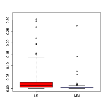
A.2 Proof of Theorem 3.5

Let denote as Θ=×q×r1××rpΘsuperscript𝑞subscriptsubscript𝑟1subscriptsubscript𝑟𝑝\Theta=\mathbb{R}\times\mathbb{R}^{q}\times{\mathcal{H}}_{r_{1}}\times\dots\times{\mathcal{H}}_{r_{p}} and as Θn={𝐭Θ:gj𝒮j,1jp,π(𝐭,𝜽)ϵ0}subscriptΘ𝑛conditional-set𝐭Θformulae-sequenceformulae-sequencesubscript𝑔𝑗subscript𝒮𝑗1𝑗𝑝𝜋𝐭𝜽subscriptitalic-ϵ0\Theta_{n}=\left\{\mathbf{t}\in\Theta:g_{j}\in{\mathcal{S}}_{j},1\leq j\leq p,\pi(\mathbf{t},\mbox{\boldmath$\theta$})\leq\epsilon_{0}\right\} where ϵ0subscriptitalic-ϵ0\epsilon_{0} is given in assumption C8. Proposition 3.4 implies that π(𝜽^,𝜽)a.s.0\pi(\widehat{\mbox{\boldmath$\theta$}},\mbox{\boldmath$\theta$})\buildrel a.s.\over{\longrightarrow}0 where 𝜽^=(μ^,𝜷^t,η^1,,η^p)t^𝜽superscript^𝜇superscript^𝜷tsubscript^𝜂1subscript^𝜂𝑝t\widehat{\mbox{\boldmath$\theta$}}=(\widehat{\mu},\widehat{\mbox{\boldmath$\beta$}}^{\mbox{\footnotesize\sc t}},\widehat{\eta}_{1},\dots,\widehat{\eta}_{p})^{\mbox{\footnotesize\sc t}} are defined through (6) and (7). Therefore, except for a null probability set, 𝜽^Θn^𝜽subscriptΘ𝑛\widehat{\mbox{\boldmath$\theta$}}\in\Theta_{n}, for n𝑛n large enough.

The following Lemma gives conditions under which C8 holds. Its proof follows the same arguments as those considered in Boente et al. (2021).

Lemma A.5.

Let ρ𝜌\rho be a function satisfying C2 and such that ρ=ψsuperscript𝜌𝜓\rho^{\prime}=\psi is continuously differentiable with bounded derivative ψsuperscript𝜓\psi^{\prime} and 𝔼ψ(ε)>0𝔼superscript𝜓𝜀0\mathbb{E}\psi^{\prime}(\varepsilon)>0. If there exists C>0𝐶0C>0 such that (𝐙C)=1norm𝐙𝐶1\mathbb{P}(\|\mathbf{Z}\|\leq C)=1, then C8 holds.

Proof. Using a Taylor expansion of order two, we have that

L(𝐭,ς)L(𝜽,ς)𝐿𝐭𝜍𝐿𝜽𝜍\displaystyle L(\mathbf{t},\varsigma)-L(\mbox{\boldmath$\theta$},\varsigma) =\displaystyle= 𝔼[ρ(Ya𝐛t𝐙j=1pgj(Xj)ς)ρ(σες)]𝔼delimited-[]𝜌𝑌𝑎superscript𝐛t𝐙superscriptsubscript𝑗1𝑝subscript𝑔𝑗subscript𝑋𝑗𝜍𝜌𝜎𝜀𝜍\displaystyle\mathbb{E}\left[\rho\left(\frac{Y-a-\mathbf{b}^{\mbox{\footnotesize\sc t}}\mathbf{Z}-\sum_{j=1}^{p}g_{j}(X_{j})}{\varsigma}\right)-\rho\left(\frac{\sigma\varepsilon}{\varsigma}\right)\right]
=\displaystyle= 𝔼[ρ(σε(aμ)(𝐛𝜷)t𝐗j=1p(gjηj)(Xj)ς)ρ(σες)]𝔼delimited-[]𝜌𝜎𝜀𝑎𝜇superscript𝐛𝜷t𝐗superscriptsubscript𝑗1𝑝subscript𝑔𝑗subscript𝜂𝑗subscript𝑋𝑗𝜍𝜌𝜎𝜀𝜍\displaystyle\mathbb{E}\left[\rho\left(\frac{\sigma\varepsilon-(a-\mu)-(\mathbf{b}-\mbox{\boldmath$\beta$})^{\mbox{\footnotesize\sc t}}\mathbf{X}-\sum_{j=1}^{p}(g_{j}-\eta_{j})(X_{j})}{\varsigma}\right)-\rho\left(\frac{\sigma\varepsilon}{\varsigma}\right)\right]
=\displaystyle= 𝔼[ψ(σες)((aμ)+(𝐛𝜷)t𝐙+j=1p(gjηj)(Xj))]𝔼delimited-[]𝜓𝜎𝜀𝜍𝑎𝜇superscript𝐛𝜷t𝐙superscriptsubscript𝑗1𝑝subscript𝑔𝑗subscript𝜂𝑗subscript𝑋𝑗\displaystyle\mathbb{E}\left[\psi\left(\frac{\sigma\varepsilon}{\varsigma}\right)\left((a-\mu)+(\mathbf{b}-\mbox{\boldmath$\beta$})^{\mbox{\footnotesize\sc t}}\mathbf{Z}+\sum_{j=1}^{p}(g_{j}-\eta_{j})(X_{j})\right)\right]
+12𝔼[ψ(σε+ξς)((aμ)+(𝐛𝜷)t𝐙+j=1p(gjηj)(Xj))2]12𝔼delimited-[]𝜓𝜎𝜀𝜉𝜍superscript𝑎𝜇superscript𝐛𝜷t𝐙superscriptsubscript𝑗1𝑝subscript𝑔𝑗subscript𝜂𝑗subscript𝑋𝑗2\displaystyle+\frac{1}{2}\mathbb{E}\left[\psi\left(\frac{\sigma\varepsilon+\xi}{\varsigma}\right)\left((a-\mu)+(\mathbf{b}-\mbox{\boldmath$\beta$})^{\mbox{\footnotesize\sc t}}\mathbf{Z}+\sum_{j=1}^{p}(g_{j}-\eta_{j})(X_{j})\right)^{2}\right]
=\displaystyle= 12𝔼[ψ(σε+ξς)((aμ)+(𝐛𝜷)t𝐙+j=1p(gjηj)(Xj))2]12𝔼delimited-[]𝜓𝜎𝜀𝜉𝜍superscript𝑎𝜇superscript𝐛𝜷t𝐙superscriptsubscript𝑗1𝑝subscript𝑔𝑗subscript𝜂𝑗subscript𝑋𝑗2\displaystyle\frac{1}{2}\mathbb{E}\left[\psi\left(\frac{\sigma\varepsilon+\xi}{\varsigma}\right)\left((a-\mu)+(\mathbf{b}-\mbox{\boldmath$\beta$})^{\mbox{\footnotesize\sc t}}\mathbf{Z}+\sum_{j=1}^{p}(g_{j}-\eta_{j})(X_{j})\right)^{2}\right]

where ξ𝜉\xi is an intermmediate point between G(𝐙,𝐗)=aμ+(𝐛𝜷)t𝐙+j=1p(gjηj)(Xj)𝐺𝐙𝐗𝑎𝜇superscript𝐛𝜷t𝐙superscriptsubscript𝑗1𝑝subscript𝑔𝑗subscript𝜂𝑗subscript𝑋𝑗G(\mathbf{Z},\mathbf{X})=a-\mu+(\mathbf{b}-\mbox{\boldmath$\beta$})^{\mbox{\footnotesize\sc t}}\mathbf{Z}+\sum_{j=1}^{p}(g_{j}-\eta_{j})(X_{j}) and 00. Noting that |(aμ)+(𝐛𝜷)t𝐙+j=1p(gjηj)(Xj)||aμ|+𝐛𝜷𝐙+j=1pgjηj𝑎𝜇superscript𝐛𝜷t𝐙superscriptsubscript𝑗1𝑝subscript𝑔𝑗subscript𝜂𝑗subscript𝑋𝑗𝑎𝜇norm𝐛𝜷norm𝐙superscriptsubscript𝑗1𝑝subscriptnormsubscript𝑔𝑗subscript𝜂𝑗|(a-\mu)+(\mathbf{b}-\mbox{\boldmath$\beta$})^{\mbox{\footnotesize\sc t}}\mathbf{Z}+\sum_{j=1}^{p}(g_{j}-\eta_{j})(X_{j})|\leq|a-\mu|+\|\mathbf{b}-\mbox{\boldmath$\beta$}\|\|\mathbf{Z}\|+\sum_{j=1}^{p}\|g_{j}-\eta_{j}\|_{\infty}, if |aμ|+𝐛𝜷+j=1pgjηj<ϵ0𝑎𝜇norm𝐛𝜷superscriptsubscript𝑗1𝑝subscriptnormsubscript𝑔𝑗subscript𝜂𝑗subscriptitalic-ϵ0|a-\mu|+\|\mathbf{b}-\mbox{\boldmath$\beta$}\|+\sum_{j=1}^{p}\|g_{j}-\eta_{j}\|_{\infty}<\epsilon_{0} and recalling that P(𝐙C)=1𝑃norm𝐙𝐶1P(\|\mathbf{Z}\|\leq C)=1, we get that |ξ|<(C+2)ϵ0𝜉𝐶2subscriptitalic-ϵ0|\xi|<(C+2)\epsilon_{0} with probability 111.

The fact that φ=𝔼ψ(ε)>0𝜑𝔼superscript𝜓𝜀0\varphi=\mathbb{E}\psi^{\prime}(\varepsilon)>0 and the continuity of ψsuperscript𝜓\psi^{\prime} entail that for δ𝛿\delta small enough

infς>0,|ςσ|<δ,|d|<δ𝔼ψ(σε+dς)>φ2>0.subscriptinfimumformulae-sequence𝜍0formulae-sequence𝜍𝜎𝛿𝑑𝛿𝔼superscript𝜓𝜎𝜀𝑑𝜍𝜑20\inf_{\varsigma>0,\,|\varsigma-\sigma|<\delta,\,|d|<\delta}\mathbb{E}\psi^{\prime}\left(\frac{\sigma\varepsilon+d}{\varsigma}\right)>\frac{\varphi}{2}>0\,.

Hence, if 𝒱={ς>0:|ςσ|<δ}𝒱conditional-set𝜍0𝜍𝜎𝛿{\mathcal{V}}=\{\varsigma>0\,:\,|\varsigma-\sigma|<\delta\} and ϵ0=δ/(C+2)subscriptitalic-ϵ0𝛿𝐶2\epsilon_{0}=\delta/(C+2), we have that

L(𝐭,ς)L(𝜽,ς)𝐿𝐭𝜍𝐿𝜽𝜍\displaystyle L(\mathbf{t},\varsigma)-L(\mbox{\boldmath$\theta$},\varsigma) =\displaystyle= 12𝔼[ψ(σε+ξς)((aμ)+(𝐛𝜷)t𝐙+j=1p(gjηj)(Xj))2]12𝔼delimited-[]superscript𝜓𝜎𝜀𝜉𝜍superscript𝑎𝜇superscript𝐛𝜷t𝐙superscriptsubscript𝑗1𝑝subscript𝑔𝑗subscript𝜂𝑗subscript𝑋𝑗2\displaystyle\frac{1}{2}\mathbb{E}\left[\psi^{\prime}\left(\frac{\sigma\varepsilon+\xi}{\varsigma}\right)\left((a-\mu)+(\mathbf{b}-\mbox{\boldmath$\beta$})^{\mbox{\footnotesize\sc t}}\mathbf{Z}+\sum_{j=1}^{p}(g_{j}-\eta_{j})(X_{j})\right)^{2}\right]
=\displaystyle= 12𝔼[((aμ)+(𝐛𝜷)t𝐙+j=1p(gjηj)(Xj))2𝔼{ψ(σε+ξς)|(𝐙,𝐗)}]12𝔼delimited-[]superscript𝑎𝜇superscript𝐛𝜷t𝐙superscriptsubscript𝑗1𝑝subscript𝑔𝑗subscript𝜂𝑗subscript𝑋𝑗2𝔼conditional-setsuperscript𝜓𝜎𝜀𝜉𝜍𝐙𝐗\displaystyle\frac{1}{2}\mathbb{E}\left[\left((a-\mu)+(\mathbf{b}-\mbox{\boldmath$\beta$})^{\mbox{\footnotesize\sc t}}\mathbf{Z}+\sum_{j=1}^{p}(g_{j}-\eta_{j})(X_{j})\right)^{2}\mathbb{E}\left\{\psi^{\prime}\left(\frac{\sigma\varepsilon+\xi}{\varsigma}\right)\Big{|}(\mathbf{Z},\mathbf{X})\right\}\right]
>\displaystyle> φ4𝔼[((aμ)+(𝐛𝜷)t𝐙+j=1p(gjηj)(Xj))2]=φ4π2(𝐭,𝜷),𝜑4𝔼delimited-[]superscript𝑎𝜇superscript𝐛𝜷t𝐙superscriptsubscript𝑗1𝑝subscript𝑔𝑗subscript𝜂𝑗subscript𝑋𝑗2𝜑4subscriptsuperscript𝜋2𝐭𝜷\displaystyle\frac{\varphi}{4}\mathbb{E}\left[\left((a-\mu)+(\mathbf{b}-\mbox{\boldmath$\beta$})^{\mbox{\footnotesize\sc t}}\mathbf{Z}+\sum_{j=1}^{p}(g_{j}-\eta_{j})(X_{j})\right)^{2}\right]=\frac{\varphi}{4}\pi^{2}_{\mathbb{P}}(\mathbf{t},\mbox{\boldmath$\beta$})\,,

concluding the proof. ∎

For each 1jp1𝑗𝑝1\leq j\leq p and 𝐜=(c1,,ckj1)tkj1𝐜superscriptsubscript𝑐1subscript𝑐subscript𝑘𝑗1tsuperscriptsubscript𝑘𝑗1\mathbf{c}=(c_{1},\dots,c_{k_{j}-1})^{\mbox{\footnotesize\sc t}}\in\mathbb{R}^{k_{j}-1}, to strength the dependence on the coefficients cssubscript𝑐𝑠c_{s}, 1skj11𝑠subscript𝑘𝑗11\leq s\leq k_{j}-1, we denote gj,𝐜(x)=s=1kj1csBs(j)(x)subscript𝑔𝑗𝐜𝑥superscriptsubscript𝑠1subscript𝑘𝑗1subscript𝑐𝑠superscriptsubscript𝐵𝑠𝑗𝑥g_{j,\mathbf{c}}(x)=\sum_{s=1}^{k_{j}-1}c_{s}B_{s}^{(j)}(x). In order to prove Theorem 3.5, we will need the following Lemma whose proof follows similar arguments to those considered in Lemma S.2.5 in Boente et al. (2020).

Lemma A.6.

Let ρ𝜌\rho be a function satisfying C2. Given fixed values 𝐜0,jkj1subscript𝐜0𝑗superscriptsubscript𝑘𝑗1\mathbf{c}_{0,j}\in\mathbb{R}^{k_{j}-1}, 1jp1𝑗𝑝1\leq j\leq p, let 𝐭0=(μ,𝛃t,g0,1,,g0,p)t×q×𝒮1××𝒮psubscript𝐭0superscript𝜇superscript𝛃tsubscript𝑔01subscript𝑔0𝑝tsuperscript𝑞subscript𝒮1subscript𝒮𝑝\mathbf{t}_{0}=(\mu,\mbox{\boldmath$\beta$}^{\mbox{\footnotesize\sc t}},g_{0,1},\dots,g_{0,p})^{\mbox{\footnotesize\sc t}}\in\mathbb{R}\times\mathbb{R}^{q}\times{\mathcal{S}}_{1}\times\dots\times{\mathcal{S}}_{p} be such that g0,j=gj,𝐜0,jsubscript𝑔0𝑗subscript𝑔𝑗subscript𝐜0𝑗g_{0,j}=g_{j,\mathbf{c}_{0,j}}. Define the class of functions

𝒢n,κ,𝐭,𝐭0={f𝐭,ς=V𝐭,ςV𝐭,ς:π(𝐭,𝐭0)<κ,𝐭Θn,ς𝒱=[σ1,σ2]}subscript𝒢𝑛𝜅superscript𝐭subscript𝐭0conditional-setsubscript𝑓𝐭𝜍subscript𝑉𝐭𝜍subscript𝑉superscript𝐭𝜍formulae-sequence𝜋𝐭subscript𝐭0𝜅formulae-sequence𝐭subscriptΘ𝑛𝜍𝒱subscript𝜎1subscript𝜎2{\mathcal{G}}_{n,\kappa,\mathbf{t}^{\star},\mathbf{t}_{0}}=\left\{f_{\mathbf{t},\varsigma}=V_{\mathbf{t},\varsigma}-V_{\mathbf{t}^{\star},\varsigma}\,:\,\pi(\mathbf{t},\mathbf{t}_{0})<\kappa,\,\mathbf{t}\in\Theta_{n},\,\varsigma\in{\mathcal{V}}=[\sigma_{1},\sigma_{2}]\right\}

with σ1=σ/2subscript𝜎1𝜎2\sigma_{1}=\sigma/2, σ2=(3/2)σsubscript𝜎232𝜎\sigma_{2}=(3/2)\sigma, 𝐭=(a,𝐛,g1,,gp)Θsuperscript𝐭superscript𝑎superscript𝐛superscriptsubscript𝑔1superscriptsubscript𝑔𝑝Θ\mathbf{t}^{\star}=(a^{\star},\mathbf{b}^{\star},g_{1}^{\star},\dots,g_{p}^{\star})\in\Theta is a fixed point and

V𝐭,ς=V𝐭,ς(y,𝐳,𝐱)=ρ(ya𝐛t𝐳j=1pgj(xj)ς)subscript𝑉𝐭𝜍subscript𝑉𝐭𝜍𝑦𝐳𝐱𝜌𝑦𝑎superscript𝐛t𝐳superscriptsubscript𝑗1𝑝subscript𝑔𝑗subscript𝑥𝑗𝜍V_{\mathbf{t},\varsigma}=V_{\mathbf{t},\varsigma}(y,\mathbf{z},\mathbf{x})=\rho\left(\frac{y-a-\mathbf{b}^{\mbox{\footnotesize\sc t}}\mathbf{z}-\sum_{j=1}^{p}g_{j}(x_{j})}{\varsigma}\right)

for 𝐭=(a,𝐛t,g1,,gp)t𝐭superscript𝑎superscript𝐛tsubscript𝑔1subscript𝑔𝑝t\mathbf{t}=(a,\mathbf{b}^{\mbox{\footnotesize\sc t}},g_{1},\dots,g_{p})^{\mbox{\footnotesize\sc t}}. Assume that 𝔼𝐙2<𝔼superscriptnorm𝐙2\mathbb{E}\|\mathbf{Z}\|^{2}<\infty. Then, there exists some constants A>0𝐴0A>0 and Asuperscript𝐴A^{\star} independent of n𝑛n, 𝐜0,jsubscript𝐜0𝑗\mathbf{c}_{0,j} and ϵitalic-ϵ\epsilon such that

N[](ϵ,𝒢n,κ,𝐭,𝐭0,L2(P))A(Amax(1,κ)ϵ)K+p+q+2.subscript𝑁italic-ϵsubscript𝒢𝑛𝜅superscript𝐭subscript𝐭0subscript𝐿2𝑃𝐴superscriptsuperscript𝐴1𝜅italic-ϵ𝐾𝑝𝑞2N_{[\,\,]}\left(\epsilon,{\mathcal{G}}_{n,\kappa,\mathbf{t}^{\star},\mathbf{t}_{0}},L_{2}(P)\right)\leq A\left(\frac{A^{\star}\max(1,\kappa)}{\epsilon}\right)^{K+p+q+2}\,.

Proof. First note that, for any g𝒮j𝑔subscript𝒮𝑗g\in{\mathcal{S}}_{j}, there exists 𝐜=(c1,,ckj1)tkj1𝐜superscriptsubscript𝑐1subscript𝑐subscript𝑘𝑗1tsuperscriptsubscript𝑘𝑗1\mathbf{c}=(c_{1},\dots,c_{k_{j}-1})^{\mbox{\footnotesize\sc t}}\in\mathbb{R}^{k_{j}-1}, such that g(x)=g𝐜(x)=s=1kj1csBs(j)(x)𝑔𝑥subscript𝑔𝐜𝑥superscriptsubscript𝑠1subscript𝑘𝑗1subscript𝑐𝑠superscriptsubscript𝐵𝑠𝑗𝑥g(x)=g_{\mathbf{c}}(x)=\sum_{s=1}^{k_{j}-1}c_{s}B_{s}^{(j)}(x). Furthermore, taking into account that Bs(j)(x)=B~s(j)(x)jB~s(j)(x)𝑑xsuperscriptsubscript𝐵𝑠𝑗𝑥superscriptsubscript~𝐵𝑠𝑗𝑥subscriptsubscript𝑗superscriptsubscript~𝐵𝑠𝑗𝑥differential-d𝑥B_{s}^{(j)}(x)=\widetilde{B}_{s}^{(j)}(x)-\int_{{\mathcal{I}}_{j}}\widetilde{B}_{s}^{(j)}(x)dx and that s=1kjB~s(j)(x)=1superscriptsubscript𝑠1subscript𝑘𝑗superscriptsubscript~𝐵𝑠𝑗𝑥1\sum_{s=1}^{k_{j}}\widetilde{B}_{s}^{(j)}(x)=1, we get that

g𝐜(x)subscript𝑔𝐜𝑥\displaystyle g_{\mathbf{c}}(x) =s=1kj1csBs(j)(x)=s=1kj1csB~s(j)(x)s=1kj1csjB~s(j)(t)𝑑tabsentsuperscriptsubscript𝑠1subscript𝑘𝑗1subscript𝑐𝑠superscriptsubscript𝐵𝑠𝑗𝑥superscriptsubscript𝑠1subscript𝑘𝑗1subscript𝑐𝑠superscriptsubscript~𝐵𝑠𝑗𝑥superscriptsubscript𝑠1subscript𝑘𝑗1subscript𝑐𝑠subscriptsubscript𝑗superscriptsubscript~𝐵𝑠𝑗𝑡differential-d𝑡\displaystyle=\sum_{s=1}^{k_{j}-1}c_{s}B_{s}^{(j)}(x)=\sum_{s=1}^{k_{j}-1}c_{s}\widetilde{B}_{s}^{(j)}(x)-\sum_{s=1}^{k_{j}-1}c_{s}\int_{{\mathcal{I}}_{j}}\widetilde{B}_{s}^{(j)}(t)dt
=s=1kj1csB~s(j)(x){=1kj1cjB~(j)(t)𝑑t}s=1kjB~s(j)(x)=s=1kjλs,𝐜B~s(j)(x),absentsuperscriptsubscript𝑠1subscript𝑘𝑗1subscript𝑐𝑠superscriptsubscript~𝐵𝑠𝑗𝑥superscriptsubscript1subscript𝑘𝑗1subscript𝑐subscriptsubscript𝑗superscriptsubscript~𝐵𝑗𝑡differential-d𝑡superscriptsubscript𝑠1subscript𝑘𝑗superscriptsubscript~𝐵𝑠𝑗𝑥superscriptsubscript𝑠1subscript𝑘𝑗subscript𝜆𝑠𝐜superscriptsubscript~𝐵𝑠𝑗𝑥\displaystyle=\sum_{s=1}^{k_{j}-1}c_{s}\widetilde{B}_{s}^{(j)}(x)-\left\{\sum_{\ell=1}^{k_{j}-1}c_{\ell}\int_{{\mathcal{I}}_{j}}\widetilde{B}_{\ell}^{(j)}(t)dt\right\}\sum_{s=1}^{k_{j}}\widetilde{B}_{s}^{(j)}(x)=\sum_{s=1}^{k_{j}}\lambda_{s,\mathbf{c}}\widetilde{B}_{s}^{(j)}(x)\,,

where λs,𝐜=cs=1kj1cjB~(j)(t)𝑑tsubscript𝜆𝑠𝐜subscript𝑐𝑠superscriptsubscript1subscript𝑘𝑗1subscript𝑐subscriptsubscript𝑗superscriptsubscript~𝐵𝑗𝑡differential-d𝑡\lambda_{s,\mathbf{c}}=c_{s}-\sum_{\ell=1}^{k_{j}-1}c_{\ell}\int_{{\mathcal{I}}_{j}}\widetilde{B}_{\ell}^{(j)}(t)dt, for 1skj11𝑠subscript𝑘𝑗11\leq s\leq k_{j}-1 and λkj,𝐜==1kj1cjB~(j)(t)𝑑tsubscript𝜆subscript𝑘𝑗𝐜superscriptsubscript1subscript𝑘𝑗1subscript𝑐subscriptsubscript𝑗superscriptsubscript~𝐵𝑗𝑡differential-d𝑡\lambda_{k_{j},\mathbf{c}}=\,-\,\sum_{\ell=1}^{k_{j}-1}c_{\ell}\int_{{\mathcal{I}}_{j}}\widetilde{B}_{\ell}^{(j)}(t)dt. Therefore, there exists a constant Djsubscript𝐷𝑗D_{j}, Dj1subscript𝐷𝑗1D_{j}\leq 1, depending only on the degree jsubscript𝑗\ell_{j} of the considered splines such that

Dj𝝀𝐜g𝐜𝝀𝐜subscript𝐷𝑗subscriptnormsubscript𝝀𝐜subscriptnormsubscript𝑔𝐜subscriptnormsubscript𝝀𝐜D_{j}\|\mbox{\boldmath$\lambda$}_{\mathbf{c}}\|_{\infty}\leq\|g_{\mathbf{c}}\|_{\infty}\leq\|\mbox{\boldmath$\lambda$}_{\mathbf{c}}\|_{\infty} (A.17)

where 𝝀𝐜=(λ1,𝐜,,λkj,𝐜)tsubscript𝝀𝐜superscriptsubscript𝜆1𝐜subscript𝜆subscript𝑘𝑗𝐜t\mbox{\boldmath$\lambda$}_{\mathbf{c}}=(\lambda_{1,\mathbf{c}},\dots,\lambda_{k_{j},\mathbf{c}})^{\mbox{\footnotesize\sc t}} and for a vector 𝐚k𝐚superscript𝑘\mathbf{a}\in\mathbb{R}^{k}, 𝐚=max1sk|as|subscriptnorm𝐚subscript1𝑠𝑘subscript𝑎𝑠\|\mathbf{a}\|_{\infty}=\max_{1\leq s\leq k}|a_{s}| (see de Boor, 1973, Section 3).

Thus if we denote as

κ,g0,j(j)superscriptsubscript𝜅subscript𝑔0𝑗𝑗\displaystyle{\mathcal{H}}_{\kappa,g_{0,j}}^{(j)} ={g𝐜(x)=s=1kj1csBs(j)(x),𝐜kj1,g𝐜g0,jκ}.absentformulae-sequencesubscript𝑔𝐜𝑥superscriptsubscript𝑠1subscript𝑘𝑗1subscript𝑐𝑠superscriptsubscript𝐵𝑠𝑗𝑥formulae-sequence𝐜superscriptsubscript𝑘𝑗1subscriptnormsubscript𝑔𝐜subscript𝑔0𝑗𝜅\displaystyle=\left\{g_{\mathbf{c}}(x)=\sum_{s=1}^{k_{j}-1}c_{s}B_{s}^{(j)}(x)\,,\mathbf{c}\in\mathbb{R}^{k_{j}-1},\|g_{\mathbf{c}}-g_{0,j}\|_{\infty}\leq\kappa\right\}\,.

we have that κ,g0,j(j){s=1kjasB~s(j)(x),𝐚𝝀0,kj(κ1)}superscriptsubscript𝜅subscript𝑔0𝑗𝑗superscriptsubscript𝑠1subscript𝑘𝑗subscript𝑎𝑠superscriptsubscript~𝐵𝑠𝑗𝑥𝐚subscriptsubscript𝝀0subscript𝑘𝑗subscript𝜅1{\mathcal{H}}_{\kappa,g_{0,j}}^{(j)}\subset\{\sum_{s=1}^{k_{j}}a_{s}\widetilde{B}_{s}^{(j)}(x),\mathbf{a}\in{\mathcal{B}}_{\mbox{\footnotesize$\mbox{\boldmath$\lambda$}$}_{0},k_{j}}(\kappa_{1})\} with κ1=κ/Dsubscript𝜅1𝜅𝐷\kappa_{1}=\kappa/D, D=min1jpDj𝐷subscript1𝑗𝑝subscript𝐷𝑗D=\min_{1\leq j\leq p}D_{j}, 𝝀0,kj(δ)={𝐚kj:𝐚𝝀0<δ}subscriptsubscript𝝀0subscript𝑘𝑗𝛿conditional-set𝐚superscriptsubscript𝑘𝑗subscriptnorm𝐚subscript𝝀0𝛿{\mathcal{B}}_{\mbox{\footnotesize$\mbox{\boldmath$\lambda$}$}_{0},k_{j}}(\delta)=\{\mathbf{a}\in\mathbb{R}^{k_{j}}:\|\mathbf{a}-\mbox{\boldmath$\lambda$}_{0}\|_{\infty}<\delta\}, 𝐚=(a1,,akj)t𝐚superscriptsubscript𝑎1subscript𝑎subscript𝑘𝑗t\mathbf{a}=(a_{1},\dots,a_{k_{j}})^{\mbox{\footnotesize\sc t}} and 𝝀0=𝝀𝐜0subscript𝝀0subscript𝝀subscript𝐜0\mbox{\boldmath$\lambda$}_{0}=\mbox{\boldmath$\lambda$}_{\mathbf{c}_{0}}.

Recall that the ball 𝝀0,k(δ)subscriptsubscript𝝀0𝑘𝛿{\mathcal{B}}_{\mbox{\footnotesize$\mbox{\boldmath$\lambda$}$}_{0},k}(\delta) can be covered by at most {(4δ+ϵ)/ϵ}ksuperscript4𝛿italic-ϵitalic-ϵ𝑘\{(4\delta+\epsilon)/\epsilon\}^{k} balls of radius ϵitalic-ϵ\epsilon, when ϵ<δitalic-ϵ𝛿\epsilon<\delta, while if ϵ>δitalic-ϵ𝛿\epsilon>\delta the covering number equals 111. Hence, using the upper bounds given in (A.17) and using that for any class of functions {\mathcal{H}}, N[](ϵ,,L)N(ϵ,,L)subscript𝑁italic-ϵsubscript𝐿𝑁italic-ϵsubscript𝐿N_{[\,\,]}(\epsilon,{\mathcal{H}},L_{\infty})\leq N(\epsilon,{\mathcal{H}},L_{\infty}), we obtain that

logN[](ϵ,κ,g0,j(j),L)kjlog(5κ1/ϵ)subscript𝑁italic-ϵsuperscriptsubscript𝜅subscript𝑔0𝑗𝑗subscript𝐿subscript𝑘𝑗5subscript𝜅1italic-ϵ\log N_{[\,\,]}(\epsilon,{\mathcal{H}}_{\kappa,g_{0,j}}^{(j)},L_{\infty})\leq k_{j}\log(5\,\kappa_{1}/\epsilon) (A.18)

for 0<ϵ<κ10italic-ϵsubscript𝜅10<\epsilon<\kappa_{1}. Henceforth, using (A.18), we get that, for any 0<ϵ<κ10italic-ϵsubscript𝜅10<\epsilon<\kappa_{1}, κ,g0,j(j)superscriptsubscript𝜅subscript𝑔0𝑗𝑗{\mathcal{H}}_{\kappa,g_{0,j}}^{(j)} can be covered by a finite number Mj(ϵ)(5(κ1)/ϵ)kjsubscript𝑀𝑗italic-ϵsuperscript5subscript𝜅1italic-ϵsubscript𝑘𝑗M_{j}(\epsilon)\leq(5(\kappa_{1})/\epsilon)^{k_{j}} of ϵlimit-fromitalic-ϵ\epsilon-brackets {[g,L(j),g,U(j)],1Mj(ϵ)}superscriptsubscript𝑔𝐿𝑗superscriptsubscript𝑔𝑈𝑗1subscript𝑀𝑗italic-ϵ\{[g_{\ell,L}^{(j)},g_{\ell,U}^{(j)}],1\leq\ell\leq M_{j}(\epsilon)\}, 1jp1𝑗𝑝1\leq j\leq p, that is, for any gκ,g0,j(j)𝑔superscriptsubscript𝜅subscript𝑔0𝑗𝑗g\in{\mathcal{H}}_{\kappa,g_{0,j}}^{(j)}, we have that g,L(j)gg,U(j)superscriptsubscript𝑔𝐿𝑗𝑔superscriptsubscript𝑔𝑈𝑗g_{\ell,L}^{(j)}\leq g\leq g_{\ell,U}^{(j)} and g,U(j)g,L(j)<ϵsubscriptnormsuperscriptsubscript𝑔𝑈𝑗superscriptsubscript𝑔𝐿𝑗italic-ϵ\|g_{\ell,U}^{(j)}-g_{\ell,L}^{(j)}\|_{\infty}<\epsilon.

Analogously, the ball μ,1(δ)subscript𝜇1𝛿{\mathcal{B}}_{\mu,1}(\delta) can be covered by at most (4δ+ϵ)/ϵ4𝛿italic-ϵitalic-ϵ(4\delta+\epsilon)/\epsilon balls of radius ϵitalic-ϵ\epsilon and 𝜷,q(2)(δ)superscriptsubscript𝜷𝑞2𝛿{\mathcal{B}}_{\mbox{\scriptsize${\mbox{\boldmath$\beta$}}$},q}^{(2)}(\delta) by at most {(4δ+ϵ)/ϵ}qsuperscript4𝛿italic-ϵitalic-ϵ𝑞\{(4\delta+\epsilon)/\epsilon\}^{q}, where 𝜷,q(2)(δ)={𝐛q:𝐛𝜷<δ}superscriptsubscript𝜷𝑞2𝛿conditional-set𝐛superscript𝑞norm𝐛𝜷𝛿{\mathcal{B}}_{\mbox{\scriptsize${\mbox{\boldmath$\beta$}}$},q}^{(2)}(\delta)=\{\mathbf{b}\in\mathbb{R}^{q}:\|\mathbf{b}-\mbox{\boldmath$\beta$}\|<\delta\} is the usual euclidean ball. Note that for any f𝐭,ς𝒢n,κ,𝐭,𝐭0subscript𝑓𝐭𝜍subscript𝒢𝑛𝜅superscript𝐭subscript𝐭0f_{\mathbf{t},\varsigma}\in{\mathcal{G}}_{n,\kappa,\mathbf{t}^{\star},\mathbf{t}_{0}} we have that aμ,1(κ)𝑎subscript𝜇1𝜅a\in{\mathcal{B}}_{\mu,1}(\kappa), 𝐛𝜷,q(2)(κ)𝐛superscriptsubscript𝜷𝑞2𝜅\mathbf{b}\in{\mathcal{B}}_{\mbox{\scriptsize${\mbox{\boldmath$\beta$}}$},q}^{(2)}(\kappa). Thus, for any 0<ϵ<κ0italic-ϵ𝜅0<\epsilon<\kappa, μ,1(κ)subscript𝜇1𝜅{\mathcal{B}}_{\mu,1}(\kappa) can be covered by a finite number Ma0(ϵ)5κ/ϵsubscript𝑀subscript𝑎0italic-ϵ5𝜅italic-ϵM_{a_{0}}(\epsilon)\leq 5\kappa/\epsilon of ϵlimit-fromitalic-ϵ\epsilon-balls with centers a(r)superscript𝑎𝑟a^{(r)}, 1rMa0(ϵ)1𝑟subscript𝑀subscript𝑎0italic-ϵ1\leq r\leq M_{a_{0}}(\epsilon). Similarly, 𝜷,q(2)(κ)superscriptsubscript𝜷𝑞2𝜅{\mathcal{B}}_{\mbox{\scriptsize${\mbox{\boldmath$\beta$}}$},q}^{(2)}(\kappa) can be covered by a finite number M𝜷(ϵ)(5κ/ϵ)qsubscript𝑀𝜷italic-ϵsuperscript5𝜅italic-ϵ𝑞M_{\mbox{\scriptsize${\mbox{\boldmath$\beta$}}$}}(\epsilon)\leq(5\kappa/\epsilon)^{q} of ϵlimit-fromitalic-ϵ\epsilon-balls of centers 𝐛(m)superscript𝐛𝑚\mathbf{b}^{(m)}.

On the other hand, the set 𝒱=[σ1,σ2]={ς:|ςσ|σ/2}𝒱subscript𝜎1subscript𝜎2conditional-set𝜍𝜍𝜎𝜎2{\mathcal{V}}=[\sigma_{1},\sigma_{2}]=\{\varsigma\,:\,|\varsigma-\sigma|\leq\sigma/2\} can be covered by Mσ(ϵ)Cσ(1/ϵ)subscript𝑀𝜎italic-ϵsubscript𝐶𝜎1italic-ϵM_{\sigma}(\epsilon)\leq C_{\sigma}(1/\epsilon) balls of radius ϵitalic-ϵ\epsilon (when ϵ<σ/2italic-ϵ𝜎2\epsilon<\sigma/2) and centers σ(s)superscript𝜎𝑠\sigma^{(s)}, 1sMσ(ϵ)1𝑠subscript𝑀𝜎italic-ϵ1\leq s\leq M_{\sigma}(\epsilon), where Cσ=3σsubscript𝐶𝜎3𝜎C_{\sigma}=3\sigma.

Recall that ψ𝜓\psi is bounded, so that, for ς𝒱𝜍𝒱\varsigma\in{\mathcal{V}},

|uρ(yuς)|ψς2ψσ.𝑢𝜌𝑦𝑢𝜍subscriptnorm𝜓𝜍2subscriptnorm𝜓𝜎\left|\frac{\partial}{\partial u}\rho\left(\frac{y-u}{\varsigma}\right)\right|\leq\frac{\|\psi\|_{\infty}}{\varsigma}\leq 2\frac{\|\psi\|_{\infty}}{\sigma}\,.

Define ϵ1=ϵ/A1subscriptitalic-ϵ1italic-ϵsubscript𝐴1\epsilon_{1}=\epsilon/A_{1} where

A1=4σ[ψ(1+(𝔼𝐙2)1/2+p)+2ζ].subscript𝐴14𝜎delimited-[]subscriptnorm𝜓1superscript𝔼superscriptnorm𝐙212𝑝2subscriptnorm𝜁A_{1}=\frac{4}{\sigma}\left[\|\psi\|_{\infty}(1+(\mathbb{E}\|\mathbf{Z}\|^{2})^{1/2}+p)+2\|\zeta\|_{\infty}\right]\,.

Given f𝐭,ς𝒢n,κ,𝐭,𝐭0subscript𝑓𝐭𝜍subscript𝒢𝑛𝜅superscript𝐭subscript𝐭0f_{\mathbf{t},\varsigma}\in{\mathcal{G}}_{n,\kappa,\mathbf{t}^{\star},\mathbf{t}_{0}}, let r𝑟r, m𝑚m, \ell and s𝑠s be such that 1rMμ(ϵ1)1𝑟subscript𝑀𝜇subscriptitalic-ϵ11\leq r\leq M_{\mu}(\epsilon_{1}), 1mM𝜷(ϵ1)1𝑚subscript𝑀𝜷subscriptitalic-ϵ11\leq m\leq M_{\mbox{\scriptsize${\mbox{\boldmath$\beta$}}$}}(\epsilon_{1}), 1Mj(ϵ1)1subscript𝑀𝑗subscriptitalic-ϵ11\leq\ell\leq M_{j}(\epsilon_{1}) and 1sMσ(ϵ1)1𝑠subscript𝑀𝜎subscriptitalic-ϵ11\leq s\leq M_{\sigma}(\epsilon_{1}) and |aa(r)|<ϵ1𝑎superscript𝑎𝑟subscriptitalic-ϵ1|a-a^{(r)}|<\epsilon_{1}, 𝐛𝐛(m)<ϵ1norm𝐛superscript𝐛𝑚subscriptitalic-ϵ1\|\mathbf{b}-\mathbf{b}^{(m)}\|<\epsilon_{1}, for 1jp1𝑗𝑝1\leq j\leq p, gj[g,L(j),g,U(j)]subscript𝑔𝑗superscriptsubscript𝑔𝐿𝑗superscriptsubscript𝑔𝑈𝑗g_{j}\in[g_{\ell,L}^{(j)},g_{\ell,U}^{(j)}] with g,U(j)g,L(j)<ϵ1subscriptnormsuperscriptsubscript𝑔𝑈𝑗superscriptsubscript𝑔𝐿𝑗subscriptitalic-ϵ1\|g_{\ell,U}^{(j)}-g_{\ell,L}^{(j)}\|_{\infty}<\epsilon_{1} and |ςσ(s)|<ϵ1𝜍superscript𝜎𝑠subscriptitalic-ϵ1|\varsigma-\sigma^{(s)}|<\epsilon_{1}. Denote as

fr,m,,ς(y,𝐳,𝐱)=ρ(ya(r)𝐛(m)t𝐳j=1pg,U(j)(xj)ς)ρ(ya𝐛t𝐳j=1pgj(xj)ς).subscript𝑓𝑟𝑚𝜍𝑦𝐳𝐱𝜌𝑦superscript𝑎𝑟superscript𝐛𝑚t𝐳superscriptsubscript𝑗1𝑝superscriptsubscript𝑔𝑈𝑗subscript𝑥𝑗𝜍𝜌𝑦superscript𝑎superscript𝐛absentt𝐳superscriptsubscript𝑗1𝑝superscriptsubscript𝑔𝑗subscript𝑥𝑗𝜍f_{r,m,\ell,\varsigma}(y,\mathbf{z},\mathbf{x})=\rho\left(\frac{y-a^{(r)}-\mathbf{b}^{(m)\mbox{\footnotesize{\sc t}}}\mathbf{z}-\sum_{j=1}^{p}g_{\ell,U}^{(j)}(x_{j})}{\varsigma}\right)-\rho\left(\frac{y-a^{\star}-\mathbf{b}^{\star\,\mbox{\footnotesize{\sc t}}}\mathbf{z}-\sum_{j=1}^{p}g_{j}^{\star}(x_{j})}{\varsigma}\right)\,.

Using a Taylor’s expansion of order one and the fact that ζ(u)=uψ(u)𝜁𝑢𝑢𝜓𝑢\zeta(u)=u\psi(u) is bounded, we get that

|f𝐭,ςfr,m,,σ(s)|subscript𝑓𝐭𝜍subscript𝑓𝑟𝑚superscript𝜎𝑠\displaystyle|f_{\mathbf{t},\varsigma}-f_{r,m,\ell,\sigma^{(s)}}| \displaystyle\leq |f𝐭,ςfr,m,,ς|+|fr,m,,ςfr,m,,σ(s)|subscript𝑓𝐭𝜍subscript𝑓𝑟𝑚𝜍subscript𝑓𝑟𝑚𝜍subscript𝑓𝑟𝑚superscript𝜎𝑠\displaystyle|f_{\mathbf{t},\varsigma}-f_{r,m,\ell,\varsigma}|+|f_{r,m,\ell,\varsigma}-f_{r,m,\ell,\sigma^{(s)}}|
\displaystyle\leq 2σψ(|aa(r)|+𝐛𝐛(m)𝐙+j=1pgjg,U(j))+limit-from2𝜎subscriptnorm𝜓𝑎superscript𝑎𝑟norm𝐛superscript𝐛𝑚norm𝐙superscriptsubscript𝑗1𝑝subscriptnormsubscript𝑔𝑗superscriptsubscript𝑔𝑈𝑗\displaystyle\frac{2}{\sigma}\|\psi\|_{\infty}\left(|a-a^{(r)}|+\|\mathbf{b}-\mathbf{b}^{(m)}\|\|\mathbf{Z}\|+\sum_{j=1}^{p}\|g_{j}-g_{\ell,U}^{(j)}\|_{\infty}\right)+
4ζσ|ςσ(s)|4subscriptnorm𝜁𝜎𝜍superscript𝜎𝑠\displaystyle 4\frac{\|\zeta\|_{\infty}}{\sigma}|\varsigma-\sigma^{(s)}|
\displaystyle\leq ϵ12σ{ψ(1+𝐙+p)+2ζ}subscriptitalic-ϵ12𝜎subscriptnorm𝜓1norm𝐙𝑝2subscriptnorm𝜁\displaystyle\epsilon_{1}\frac{2}{\sigma}\left\{\|\psi\|_{\infty}(1+\|\mathbf{Z}\|+p)+2\|\zeta\|_{\infty}\right\}

Define the functions

ϕr,m,,s(U)(y,𝐳,𝐱)superscriptsubscriptitalic-ϕ𝑟𝑚𝑠𝑈𝑦𝐳𝐱\displaystyle\phi_{r,m,\ell,s}^{(U)}(y,\mathbf{z},\mathbf{x}) =\displaystyle= fr,m,,σ(s)(y,𝐳,𝐱)+ϵ12σ{ψ(1+𝐙+p)+2ζ}subscript𝑓𝑟𝑚superscript𝜎𝑠𝑦𝐳𝐱subscriptitalic-ϵ12𝜎subscriptnorm𝜓1norm𝐙𝑝2subscriptnorm𝜁\displaystyle f_{r,m,\ell,\sigma^{(s)}}(y,\mathbf{z},\mathbf{x})+\epsilon_{1}\frac{2}{\sigma}\left\{\|\psi\|_{\infty}(1+\|\mathbf{Z}\|+p)+2\|\zeta\|_{\infty}\right\}
ϕr,m,,s(L)(y,𝐳,𝐱)superscriptsubscriptitalic-ϕ𝑟𝑚𝑠𝐿𝑦𝐳𝐱\displaystyle\phi_{r,m,\ell,s}^{(L)}(y,\mathbf{z},\mathbf{x}) =\displaystyle= fr,m,,σ(s)(y,𝐳,𝐱)ϵ12σ{ψ(1+𝐙+p)+2ζ}.subscript𝑓𝑟𝑚superscript𝜎𝑠𝑦𝐳𝐱subscriptitalic-ϵ12𝜎subscriptnorm𝜓1norm𝐙𝑝2subscriptnorm𝜁\displaystyle f_{r,m,\ell,\sigma^{(s)}}(y,\mathbf{z},\mathbf{x})-\epsilon_{1}\frac{2}{\sigma}\left\{\|\psi\|_{\infty}(1+\|\mathbf{Z}\|+p)+2\|\zeta\|_{\infty}\right\}\,.

Then we have that ϕr,m,,s(L)f𝐭,ςϕr,m,,s(U)superscriptsubscriptitalic-ϕ𝑟𝑚𝑠𝐿subscript𝑓𝐭𝜍superscriptsubscriptitalic-ϕ𝑟𝑚𝑠𝑈\phi_{r,m,\ell,s}^{(L)}\leq f_{\mathbf{t},\varsigma}\leq\phi_{r,m,\ell,s}^{(U)} and since 𝔼𝐙2<𝔼superscriptnorm𝐙2\mathbb{E}\|\mathbf{Z}\|^{2}<\infty, we obtain

ϕr,m,,s(U)ϕr,m,,s(L)L2(P)ϵ14σ[ψ(1+(𝔼𝐙2)1/2+p)+2ζ]=ϵ.subscriptnormsuperscriptsubscriptitalic-ϕ𝑟𝑚𝑠𝑈superscriptsubscriptitalic-ϕ𝑟𝑚𝑠𝐿superscript𝐿2𝑃subscriptitalic-ϵ14𝜎delimited-[]subscriptnorm𝜓1superscript𝔼superscriptnorm𝐙212𝑝2subscriptnorm𝜁italic-ϵ\|\phi_{r,m,\ell,s}^{(U)}-\phi_{r,m,\ell,s}^{(L)}\|_{L^{2}(P)}\leq\epsilon_{1}\frac{4}{\sigma}\left[\|\psi\|_{\infty}(1+(\mathbb{E}\|\mathbf{Z}\|^{2})^{1/2}+p)+2\|\zeta\|_{\infty}\right]=\epsilon\,.

Therefore, if A=3σ𝐴3𝜎A=3\sigma and A=5A1/Dsuperscript𝐴5subscript𝐴1𝐷A^{\star}=5A_{1}/D the total number of brackets of size ϵitalic-ϵ\epsilon needed to cover 𝒢n,κ,𝐭,𝐭0subscript𝒢𝑛𝜅superscript𝐭subscript𝐭0{\mathcal{G}}_{n,\kappa,\mathbf{t}^{\star},\mathbf{t}_{0}} is bounded by

Mμ,1(ϵ1)M𝜷,q(ϵ1)j=1pMj(ϵ1)Mσ(ϵ1)subscript𝑀𝜇1subscriptitalic-ϵ1subscript𝑀𝜷𝑞subscriptitalic-ϵ1superscriptsubscriptproduct𝑗1𝑝subscript𝑀𝑗subscriptitalic-ϵ1subscript𝑀𝜎subscriptitalic-ϵ1\displaystyle M_{\mu,1}(\epsilon_{1})M_{\mbox{\scriptsize${\mbox{\boldmath$\beta$}}$},q}(\epsilon_{1})\prod_{j=1}^{p}M_{j}(\epsilon_{1})\;M_{\sigma}(\epsilon_{1}) \displaystyle\leq 5κϵ1(5κϵ1)q(5κ1ϵ1)K+p3σ(1ϵ1)5𝜅subscriptitalic-ϵ1superscript5𝜅subscriptitalic-ϵ1𝑞superscript5subscript𝜅1subscriptitalic-ϵ1𝐾𝑝3𝜎1subscriptitalic-ϵ1\displaystyle\frac{5\kappa}{\epsilon_{1}}\left(\frac{5\kappa}{\epsilon_{1}}\right)^{q}\left(\frac{5\kappa_{1}}{\epsilon_{1}}\right)^{K+p}3\sigma\left(\frac{1}{\epsilon_{1}}\right)
\displaystyle\leq A(Amax(1,κ)ϵ)K+p+q+2,𝐴superscriptsuperscript𝐴1𝜅italic-ϵ𝐾𝑝𝑞2\displaystyle A\left(\frac{A^{\star}\max(1,\kappa)}{\epsilon}\right)^{K+p+q+2}\;,

where we have used that κκ1=κ/D𝜅subscript𝜅1𝜅𝐷\kappa\leq\kappa_{1}=\kappa/D since D1𝐷1D\leq 1, concluding the proof. ∎
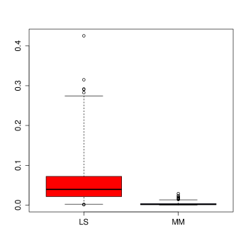
In order to prove Theorem 3.5, we need the following Lemma which is a direct consequence of Lemma A.2.3 in Boente et al. (2021). In the statement of Lemma A.7, we have in mind that Θ=×q×r1××rpΘsuperscript𝑞subscriptsubscript𝑟1subscriptsubscript𝑟𝑝\Theta=\mathbb{R}\times\mathbb{R}^{q}\times{\mathcal{H}}_{r_{1}}\times\dots\times{\mathcal{H}}_{r_{p}}, Θ~={𝐭Θ:gj𝒮j,1jp}~Θconditional-set𝐭Θformulae-sequencesubscript𝑔𝑗subscript𝒮𝑗1𝑗𝑝\widetilde{\Theta}=\left\{\mathbf{t}\in\Theta:g_{j}\in{\mathcal{S}}_{j},1\leq j\leq p\right\} and Θn={𝐭Θ~,π(𝐭,𝜽)ϵ0}subscriptΘ𝑛formulae-sequence𝐭~Θ𝜋𝐭𝜽subscriptitalic-ϵ0\Theta_{n}=\left\{\mathbf{t}\in\widetilde{\Theta},\pi(\mathbf{t},\mbox{\boldmath$\theta$})\leq\epsilon_{0}\right\} as defined above.

Lemma A.7.

Let Lnsubscript𝐿𝑛L_{n} be an stochastic process indexed by Θ~×(0,+)Θ×(0,+)~Θ0Θ0\widetilde{\Theta}\times(0,+\infty)\subset\Theta\times(0,+\infty). Furthermore, let L:Θ×(0,+):𝐿Θ0L:\Theta\times(0,+\infty)\to\mathbb{R} be a fixed function and σ^^𝜎\widehat{\sigma} an estimator of σ𝜎\sigma such that (σ^𝒱)1^𝜎𝒱1\mathbb{P}(\widehat{\sigma}\in{\mathcal{V}})\to 1 where 𝒱(0,+)𝒱0{\mathcal{V}}\subset(0,+\infty) and 𝛉nΘnΘ~subscript𝛉𝑛subscriptΘ𝑛~Θ\mbox{\boldmath$\theta$}_{n}\in\Theta_{n}\subset\widetilde{\Theta}. Let δn0subscript𝛿𝑛0\delta_{n}\geq 0 be a fixed sequence such that δn0subscript𝛿𝑛0\delta_{n}\to 0 and fix υ>0𝜐0\upsilon>0 with 0δn<υ0subscript𝛿𝑛𝜐0\leq\delta_{n}<\upsilon for all n𝑛n. Denote as 𝛉^Θ~^𝛉~Θ\widehat{\mbox{\boldmath$\theta$}}\in\widetilde{\Theta} the minimizer of Ln(𝐭,σ^)subscript𝐿𝑛𝐭^𝜎L_{n}(\mathbf{t},\widehat{\sigma}) over Θ~~Θ\widetilde{\Theta}, that is, Ln(𝛉^,σ^)Ln(𝐭,σ^)subscript𝐿𝑛^𝛉^𝜎subscript𝐿𝑛𝐭^𝜎L_{n}(\widehat{\mbox{\boldmath$\theta$}},\widehat{\sigma})\leq L_{n}(\mathbf{t},\widehat{\sigma}), for any 𝐭Θ~𝐭~Θ\mathbf{t}\in\widetilde{\Theta}. Assume that (𝛉^Θn)1^𝛉subscriptΘ𝑛1\mathbb{P}(\widehat{\mbox{\boldmath$\theta$}}\in\Theta_{n})\to 1, π(𝛉^,𝛉n)p0superscript𝑝subscript𝜋^𝛉subscript𝛉𝑛0\pi_{\mathbb{P}}(\widehat{\mbox{\boldmath$\theta$}},\mbox{\boldmath$\theta$}_{n})\buildrel p\over{\longrightarrow}0 and that there exists a function ϕnsubscriptitalic-ϕ𝑛\phi_{n} such that ϕn(δ)/δsubscriptitalic-ϕ𝑛𝛿𝛿\phi_{n}(\delta)/\delta is decreasing on (δn,)subscript𝛿𝑛(\delta_{n},\infty) and that for any δn<δυsubscript𝛿𝑛𝛿𝜐\delta_{n}<\delta\leq\upsilon, we have

sup𝐭Θn,δ,ς𝒱L(𝜽n,ς)L(𝐭,ς)subscriptsupremumformulae-sequence𝐭subscriptΘ𝑛𝛿𝜍𝒱𝐿subscript𝜽𝑛𝜍𝐿𝐭𝜍\displaystyle\sup_{\mathbf{t}\in\Theta_{n,\delta},\varsigma\in{\mathcal{V}}}L(\mbox{\boldmath$\theta$}_{n},\varsigma)-L(\mathbf{t},\varsigma) less-than-or-similar-to\displaystyle\lesssim δ2,superscript𝛿2\displaystyle-\delta^{2}\,, (A.19)
𝔼sup𝐭Θn,δ,ς𝒱n|(Ln(𝐭,ς)L(𝐭,ς))(Ln(𝜽n,ς)L(𝜽n,ς))|superscript𝔼subscriptsupremumformulae-sequence𝐭subscriptΘ𝑛𝛿𝜍𝒱𝑛subscript𝐿𝑛𝐭𝜍𝐿𝐭𝜍subscript𝐿𝑛subscript𝜽𝑛𝜍𝐿subscript𝜽𝑛𝜍\displaystyle\mathbb{E}^{*}\sup_{\mathbf{t}\in\Theta_{n,\delta},\varsigma\in{\mathcal{V}}}\sqrt{n}\left|(L_{n}(\mathbf{t},\varsigma)-L(\mathbf{t},\varsigma))-(L_{n}(\mbox{\boldmath$\theta$}_{n},\varsigma)-L(\mbox{\boldmath$\theta$}_{n},\varsigma))\right| less-than-or-similar-to\displaystyle\lesssim ϕn(δ),subscriptitalic-ϕ𝑛𝛿\displaystyle\phi_{n}(\delta)\,, (A.20)

where Θn,δ={𝐭Θn:δ/2<π(𝐭,𝛉n)δ}subscriptΘ𝑛𝛿conditional-set𝐭subscriptΘ𝑛𝛿2subscript𝜋𝐭subscript𝛉𝑛𝛿\Theta_{n,\delta}=\{\mathbf{t}\in\Theta_{n}:\delta/2<\pi_{\mathbb{P}}(\mathbf{t},\mbox{\boldmath$\theta$}_{n})\leq\delta\}, the symbol less-than-or-similar-to\lesssim means less or equal up to a universal constant and 𝔼superscript𝔼\mathbb{E}^{*} stands for the outer expectation. Then, if γnsubscript𝛾𝑛\gamma_{n} is such that δnγn=O(1)subscript𝛿𝑛subscript𝛾𝑛𝑂1\delta_{n}\,\gamma_{n}=O(1) and γn2ϕn(γn1)nsuperscriptsubscript𝛾𝑛2subscriptitalic-ϕ𝑛superscriptsubscript𝛾𝑛1𝑛\gamma_{n}^{2}\phi_{n}\left(\gamma_{n}^{-1}\right)\leq\sqrt{n}, for every n𝑛n, we have that γnπ(𝛉^,𝛉n)=O(1)subscript𝛾𝑛subscript𝜋^𝛉subscript𝛉𝑛subscript𝑂1\gamma_{n}\pi_{\mathbb{P}}(\widehat{\mbox{\boldmath$\theta$}},\mbox{\boldmath$\theta$}_{n})=O_{\mathbb{P}}(1).


Proof of Theorem 3.5. To simplify the notation from now on ρ=ρ1𝜌subscript𝜌1\rho=\rho_{1}. To derive the desired rates of convergence for the estimator 𝜽^=(μ^,𝜷^t,η^1,,η^p)t^𝜽superscript^𝜇superscript^𝜷tsubscript^𝜂1subscript^𝜂𝑝t\widehat{\mbox{\boldmath$\theta$}}=(\widehat{\mu},\widehat{\mbox{\boldmath$\beta$}}^{\mbox{\footnotesize\sc t}},\widehat{\eta}_{1},\dots,\widehat{\eta}_{p})^{\mbox{\footnotesize\sc t}} defined through (6) and (7), Lemma A.7 will be helpful.

As in the proof of Proposition 3.2, let η~~j𝒮jsubscript~~𝜂𝑗subscript𝒮𝑗\widetilde{\widetilde{\eta}}_{j}\in{\mathcal{S}}_{j} be the centered spline such that η~~jηj=O(nνjrj)subscriptnormsubscript~~𝜂𝑗subscript𝜂𝑗𝑂superscript𝑛subscript𝜈𝑗subscript𝑟𝑗\|\widetilde{\widetilde{\eta}}_{j}-\eta_{j}\|_{\infty}=O\left(n^{-\nu_{j}\,r_{j}}\right). Denote as 𝐜(j)kj1superscript𝐜𝑗superscriptsubscript𝑘𝑗1\mathbf{c}^{(j)}\in\mathbb{R}^{k_{j}-1} the vectors such that η~~j(x)=𝐜(j)𝐕(j)(x)subscript~~𝜂𝑗𝑥superscript𝐜𝑗superscript𝐕𝑗𝑥\widetilde{\widetilde{\eta}}_{j}(x)=\mathbf{c}^{(j)}\mathbf{V}^{(j)}(x) and define 𝜽n=(μ,𝜷t,η~~1,,η~~p)tsubscript𝜽𝑛superscript𝜇superscript𝜷tsubscript~~𝜂1subscript~~𝜂𝑝t\mbox{\boldmath$\theta$}_{n}=\left(\mu,\mbox{\boldmath$\beta$}^{\mbox{\footnotesize\sc t}},\widetilde{\widetilde{\eta}}_{1},\dots,\widetilde{\widetilde{\eta}}_{p}\right)^{\mbox{\footnotesize\sc t}}. Hence, for n𝑛n large enough we have that j=1pη~~jηj<min(ϵ0,1/(2A))superscriptsubscript𝑗1𝑝subscriptnormsubscript~~𝜂𝑗subscript𝜂𝑗subscriptitalic-ϵ012𝐴\sum_{j=1}^{p}\|\widetilde{\widetilde{\eta}}_{j}-\eta_{j}\|_{\infty}<\min(\epsilon_{0},1/(2A)), with ϵ0subscriptitalic-ϵ0\epsilon_{0} defined in C8 and A=4p(C0+A0)/C0𝐴4𝑝subscript𝐶0subscript𝐴0subscript𝐶0A=4\,\sqrt{p\,(C_{0}+A_{0})/C_{0}} with A0=ψ/2subscript𝐴0subscriptnormsuperscript𝜓2A_{0}=\|\psi^{\prime}\|_{\infty}/2 and C0subscript𝐶0C_{0} the constant given in C8. Hence, 𝜽nΘnsubscript𝜽𝑛subscriptΘ𝑛\mbox{\boldmath$\theta$}_{n}\in\Theta_{n}, as required in Lemma A.7.

Let δn=A{j=1pηjη~~j2}1/2subscript𝛿𝑛𝐴superscriptconditional-setsuperscriptsubscript𝑗1𝑝subscript𝜂𝑗evaluated-atsubscript~~𝜂𝑗212\delta_{n}=A\;\left\{\sum_{j=1}^{p}\|\eta_{j}-\widetilde{\widetilde{\eta}}_{j}\|_{\infty}^{2}\right\}^{1/2}, then δn<1subscript𝛿𝑛1\delta_{n}<1. Note that we can assume without loss of generality that the subset 𝒱𝒱{\mathcal{V}} in C8 is such that 𝒱[σ/2,3σ/2]𝒱𝜎23𝜎2{\mathcal{V}}\subset[\sigma/2,3\sigma/2]. Using C5, we immediately obtain that (σ^𝒱)1^𝜎𝒱1\mathbb{P}(\widehat{\sigma}\in{\mathcal{V}})\to 1. Besides, Proposition 3.4 implies that (θ^Θn)1^𝜃subscriptΘ𝑛1\mathbb{P}(\widehat{\theta}\in\Theta_{n})\to 1 as desired, while by definition 𝜽^^𝜽\widehat{\mbox{\boldmath$\theta$}} is the minimizer of Ln(𝐭,σ^)subscript𝐿𝑛𝐭^𝜎L_{n}(\mathbf{t},\widehat{\sigma}) over Θ~~Θ\widetilde{\Theta}. Hence, we only have to prove that (A.19) and (A.20) hold for any δn<δ<1subscript𝛿𝑛𝛿1\delta_{n}<\delta<1 and a proper function ϕnsubscriptitalic-ϕ𝑛\phi_{n}.

From C8 we have that for any 𝐭Θn𝐭subscriptΘ𝑛\mathbf{t}\in\Theta_{n} and ς𝒱𝜍𝒱\varsigma\in{\mathcal{V}},

L(𝐭,ς)L(𝜽,ς)C0π2(𝐭,𝜽).𝐿𝐭𝜍𝐿𝜽𝜍subscript𝐶0superscriptsubscript𝜋2𝐭𝜽L(\mathbf{t},\varsigma)-L(\mbox{\boldmath$\theta$},\varsigma)\geq C_{0}\pi_{\mathbb{P}}^{2}(\mathbf{t},\mbox{\boldmath$\theta$})\,. (A.21)

Using that ψ𝜓\psi is an odd function and that the errors have a symmetric distribution, we get that 𝔼ψ(ε/ς)=0𝔼𝜓𝜀𝜍0\mathbb{E}\psi(\varepsilon/\varsigma)=0, for any ς>0𝜍0\varsigma>0, which together with the independence between the errors and the covariates leads to

𝔼{ψ(yμ𝜷t𝐙j=1pηj(Xj)ς)j=1p(η~~j(Xj)ηj(Xj))}=0.𝔼𝜓𝑦𝜇superscript𝜷t𝐙superscriptsubscript𝑗1𝑝subscript𝜂𝑗subscript𝑋𝑗𝜍superscriptsubscript𝑗1𝑝subscript~~𝜂𝑗subscript𝑋𝑗subscript𝜂𝑗subscript𝑋𝑗0\mathbb{E}\left\{\psi\left(\frac{y-\mu-\mbox{\boldmath$\beta$}^{\mbox{\footnotesize\sc t}}\mathbf{Z}-\sum_{j=1}^{p}\eta_{j}(X_{j})}{\varsigma}\right)\sum_{j=1}^{p}\left(\widetilde{\widetilde{\eta}}_{j}(X_{j})-\eta_{j}(X_{j})\right)\right\}=0\,.

Hence, using a Taylor’s expansion of order two, we obtain

L(𝜽n,ς)L(𝜽,ς)𝐿subscript𝜽𝑛𝜍𝐿𝜽𝜍\displaystyle L(\mbox{\boldmath$\theta$}_{n},\varsigma)-L(\mbox{\boldmath$\theta$},\varsigma) =\displaystyle= 𝔼{ψ(yμ𝜷t𝐙+j=1pηj(Xj)ς)j=1p(η~~j(Xj)ηj(Xj))}𝔼𝜓𝑦𝜇superscript𝜷t𝐙superscriptsubscript𝑗1𝑝subscript𝜂𝑗subscript𝑋𝑗𝜍superscriptsubscript𝑗1𝑝subscript~~𝜂𝑗subscript𝑋𝑗subscript𝜂𝑗subscript𝑋𝑗\displaystyle\mathbb{E}\left\{\psi\left(\frac{y-\mu-\mbox{\boldmath$\beta$}^{\mbox{\footnotesize\sc t}}\mathbf{Z}+\sum_{j=1}^{p}\eta_{j}(X_{j})}{\varsigma}\right)\sum_{j=1}^{p}\left(\widetilde{\widetilde{\eta}}_{j}(X_{j})-\eta_{j}(X_{j})\right)\right\}
+\displaystyle+ 12𝔼{ψ(yμ𝜷t𝐙+j=1pξj(Xj)ς)(j=1p(η~~j(Xj)ηj(Xj)))2}12𝔼superscript𝜓𝑦𝜇superscript𝜷t𝐙superscriptsubscript𝑗1𝑝subscript𝜉𝑗subscript𝑋𝑗𝜍superscriptsuperscriptsubscript𝑗1𝑝subscript~~𝜂𝑗subscript𝑋𝑗subscript𝜂𝑗subscript𝑋𝑗2\displaystyle\frac{1}{2}\;\mathbb{E}\left\{\psi^{\prime}\left(\frac{y-\mu-\mbox{\boldmath$\beta$}^{\mbox{\footnotesize\sc t}}\mathbf{Z}+\sum_{j=1}^{p}\xi_{j}(X_{j})}{\varsigma}\right)\left(\sum_{j=1}^{p}\left(\widetilde{\widetilde{\eta}}_{j}(X_{j})-\eta_{j}(X_{j})\right)\right)^{2}\right\}
=\displaystyle= 12𝔼{ψ(yμ𝜷t𝐙+j=1pξj(Xj)ς)(j=1p(η~~j(Xj)ηj(Xj)))2}12𝔼superscript𝜓𝑦𝜇superscript𝜷t𝐙superscriptsubscript𝑗1𝑝subscript𝜉𝑗subscript𝑋𝑗𝜍superscriptsuperscriptsubscript𝑗1𝑝subscript~~𝜂𝑗subscript𝑋𝑗subscript𝜂𝑗subscript𝑋𝑗2\displaystyle\frac{1}{2}\;\mathbb{E}\left\{\psi^{\prime}\left(\frac{y-\mu-\mbox{\boldmath$\beta$}^{\mbox{\footnotesize\sc t}}\mathbf{Z}+\sum_{j=1}^{p}\xi_{j}(X_{j})}{\varsigma}\right)\left(\sum_{j=1}^{p}\left(\widetilde{\widetilde{\eta}}_{j}(X_{j})-\eta_{j}(X_{j})\right)\right)^{2}\right\}
\displaystyle\leq 12ψ𝔼(j=1p(η~~j(Xj)ηj(Xj)))212subscriptnormsuperscript𝜓𝔼superscriptsuperscriptsubscript𝑗1𝑝subscript~~𝜂𝑗subscript𝑋𝑗subscript𝜂𝑗subscript𝑋𝑗2\displaystyle\frac{1}{2}\;\|\psi^{\prime}\|_{\infty}\mathbb{E}\left(\sum_{j=1}^{p}\left(\widetilde{\widetilde{\eta}}_{j}(X_{j})-\eta_{j}(X_{j})\right)\right)^{2}
\displaystyle\leq A0(j=1pη~~jηj)2pA0j=1pη~~jηj2=j=1pO(n2rjνj),subscript𝐴0superscriptsuperscriptsubscript𝑗1𝑝subscriptnormsubscript~~𝜂𝑗subscript𝜂𝑗2𝑝subscript𝐴0superscriptsubscript𝑗1𝑝superscriptsubscriptnormsubscript~~𝜂𝑗subscript𝜂𝑗2superscriptsubscript𝑗1𝑝𝑂superscript𝑛2subscript𝑟𝑗subscript𝜈𝑗\displaystyle A_{0}\,\left(\sum_{j=1}^{p}\left\|\widetilde{\widetilde{\eta}}_{j}-\eta_{j}\right\|_{\infty}\right)^{2}\leq pA_{0}\sum_{j=1}^{p}\left\|\widetilde{\widetilde{\eta}}_{j}-\eta_{j}\right\|_{\infty}^{2}=\sum_{j=1}^{p}O(n^{-2\,r_{j}\nu_{j}})\,,

where A0=ψ/2subscript𝐴0subscriptnormsuperscript𝜓2A_{0}=\|\psi^{\prime}\|_{\infty}/2 has been defined above and ξj(Xj)subscript𝜉𝑗subscript𝑋𝑗\xi_{j}(X_{j}) is an intermediate value between ηj(Xj)subscript𝜂𝑗subscript𝑋𝑗\eta_{j}(X_{j}) and η~~j(Xj)subscript~~𝜂𝑗subscript𝑋𝑗\widetilde{\widetilde{\eta}}_{j}(X_{j}). Thus, using that

π2(𝐭,𝜽n)2π2(𝐭,𝜽)+2π2(𝜽n,𝜽)2π2(𝐭,𝜽)+2pj=1pη~~jηj2superscriptsubscript𝜋2𝐭subscript𝜽𝑛2superscriptsubscript𝜋2𝐭𝜽2superscriptsubscript𝜋2subscript𝜽𝑛𝜽2superscriptsubscript𝜋2𝐭𝜽2𝑝superscriptsubscript𝑗1𝑝superscriptsubscriptnormsubscript~~𝜂𝑗subscript𝜂𝑗2\pi_{\mathbb{P}}^{2}(\mathbf{t},\mbox{\boldmath$\theta$}_{n})\leq 2\pi_{\mathbb{P}}^{2}(\mathbf{t},\mbox{\boldmath$\theta$})+2\pi_{\mathbb{P}}^{2}(\mbox{\boldmath$\theta$}_{n},\mbox{\boldmath$\theta$})\leq 2\pi_{\mathbb{P}}^{2}(\mathbf{t},\mbox{\boldmath$\theta$})+2\,p\,\sum_{j=1}^{p}\left\|\widetilde{\widetilde{\eta}}_{j}-\eta_{j}\right\|_{\infty}^{2}

and that δ/2<π(𝐭,𝜽n)𝛿2subscript𝜋𝐭subscript𝜽𝑛\delta/2<\pi_{\mathbb{P}}(\mathbf{t},\mbox{\boldmath$\theta$}_{n}) for 𝐭Θn,δ𝐭subscriptΘ𝑛𝛿\mathbf{t}\in\Theta_{n,\delta}, together with (A.21), we obtain that

L(𝐭,ς)L(𝜽n,ς)𝐿𝐭𝜍𝐿subscript𝜽𝑛𝜍\displaystyle L(\mathbf{t},\varsigma)-L(\mbox{\boldmath$\theta$}_{n},\varsigma) L(𝐭,ς)L(𝜽,ς){L(𝜽n,ς)L(𝜽,ς)}absent𝐿𝐭𝜍𝐿𝜽𝜍𝐿subscript𝜽𝑛𝜍𝐿𝜽𝜍\displaystyle\geq L(\mathbf{t},\varsigma)-L(\mbox{\boldmath$\theta$},\varsigma)-\left\{L(\mbox{\boldmath$\theta$}_{n},\varsigma)-L(\mbox{\boldmath$\theta$},\varsigma)\right\}
C0π2(𝐭,𝜽)pA0j=1pη~~jηj2absentsubscript𝐶0superscriptsubscript𝜋2𝐭𝜽𝑝subscript𝐴0superscriptsubscript𝑗1𝑝superscriptsubscriptnormsubscript~~𝜂𝑗subscript𝜂𝑗2\displaystyle\geq C_{0}\,\pi_{\mathbb{P}}^{2}(\mathbf{t},\mbox{\boldmath$\theta$})-pA_{0}\sum_{j=1}^{p}\left\|\widetilde{\widetilde{\eta}}_{j}-\eta_{j}\right\|_{\infty}^{2}
C02π2(𝐭,𝜽n)p(C0+A0)j=1pη~~jηj2absentsubscript𝐶02superscriptsubscript𝜋2𝐭subscript𝜽𝑛𝑝subscript𝐶0subscript𝐴0superscriptsubscript𝑗1𝑝superscriptsubscriptnormsubscript~~𝜂𝑗subscript𝜂𝑗2\displaystyle\geq\frac{C_{0}}{2}\pi_{\mathbb{P}}^{2}(\mathbf{t},\mbox{\boldmath$\theta$}_{n})-p\left(C_{0}+A_{0}\right)\sum_{j=1}^{p}\left\|\widetilde{\widetilde{\eta}}_{j}-\eta_{j}\right\|_{\infty}^{2}
C08δ21A2p(C0+A0)δn2=C08δ2C016δn2C016δ2,absentsubscript𝐶08superscript𝛿21superscript𝐴2𝑝subscript𝐶0subscript𝐴0superscriptsubscript𝛿𝑛2subscript𝐶08superscript𝛿2subscript𝐶016superscriptsubscript𝛿𝑛2subscript𝐶016superscript𝛿2\displaystyle\geq\frac{C_{0}}{8}\delta^{2}-\frac{1}{A^{2}}p\left(C_{0}+A_{0}\right)\delta_{n}^{2}=\frac{C_{0}}{8}\delta^{2}-\frac{C_{0}}{16}\delta_{n}^{2}\geq\frac{C_{0}}{16}\delta^{2}\,,

where the last inequality follows from the fact that δn<δsubscript𝛿𝑛𝛿\delta_{n}<\delta. Hence, inequality (A.19) in Lemma A.7 holds.

We have to show that inequality (A.20) in in Lemma A.7 holds for a proper function ϕn(δ)subscriptitalic-ϕ𝑛𝛿\phi_{n}(\delta). Note that the left hand side of (A.20) can be bounded as

𝔼supς𝒱,𝐭Θn,δn|Ln(𝐭,ς)L(𝐭,ς)(Ln(𝜽n,ς)L(𝜽n,ς))|𝔼supfn,δn|(PnP)f|,superscript𝔼subscriptsupremumformulae-sequence𝜍𝒱𝐭subscriptΘ𝑛𝛿𝑛subscript𝐿𝑛𝐭𝜍𝐿𝐭𝜍subscript𝐿𝑛subscript𝜽𝑛𝜍𝐿subscript𝜽𝑛𝜍superscript𝔼subscriptsupremum𝑓subscript𝑛𝛿𝑛subscript𝑃𝑛𝑃𝑓\mathbb{E}^{*}\displaystyle\sup_{{\varsigma\in{\mathcal{V}}\,,}{\mathbf{t}\in\Theta_{n,\delta}}}\sqrt{n}\left|L_{n}(\mathbf{t},\varsigma)-L(\mathbf{t},\varsigma)-\left(L_{n}(\mbox{\boldmath$\theta$}_{n},\varsigma)-L(\mbox{\boldmath$\theta$}_{n},\varsigma)\right)\right|\leq\mathbb{E}^{*}\displaystyle\sup_{f\in{\mathcal{F}}_{n,\delta}}\sqrt{n}|(P_{n}-P)f|\,,

where n,δsubscript𝑛𝛿{\mathcal{F}}_{n,\delta} is the class of functions

n,δ={V𝐭,ςV𝜽n,ς:𝐭Θn,δ,ς𝒱}{V𝐭,ςV𝜽n,ς:𝐭Θn,ς𝒱},subscript𝑛𝛿conditional-setsubscript𝑉𝐭𝜍subscript𝑉subscript𝜽𝑛𝜍formulae-sequence𝐭subscriptΘ𝑛𝛿𝜍𝒱conditional-setsubscript𝑉𝐭𝜍subscript𝑉subscript𝜽𝑛𝜍formulae-sequence𝐭subscriptΘ𝑛𝜍𝒱{\mathcal{F}}_{n,\delta}=\{V_{\mathbf{t},\varsigma}-V_{\mbox{\footnotesize$\mbox{\boldmath$\theta$}$}_{n},\varsigma}:\mathbf{t}\in\Theta_{n,\delta}\,,\,\varsigma\in{\mathcal{V}}\}\subset\{V_{\mathbf{t},\varsigma}-V_{\mbox{\footnotesize$\mbox{\boldmath$\theta$}$}_{n},\varsigma}:\mathbf{t}\in\Theta_{n}\,,\,\varsigma\in{\mathcal{V}}\}\,,

and V𝐭,ςsubscript𝑉𝐭𝜍V_{\mathbf{t},\varsigma} is defined in Lemma A.6, that is,

V𝐭,ς=V𝐭,ς(y,𝐳,𝐱)=ρ(ya𝐛t𝐳j=1pgj(xj)ς).subscript𝑉𝐭𝜍subscript𝑉𝐭𝜍𝑦𝐳𝐱𝜌𝑦𝑎superscript𝐛t𝐳superscriptsubscript𝑗1𝑝subscript𝑔𝑗subscript𝑥𝑗𝜍V_{\mathbf{t},\varsigma}=V_{\mathbf{t},\varsigma}(y,\mathbf{z},\mathbf{x})=\rho\left(\frac{y-a-\mathbf{b}^{\mbox{\footnotesize\sc t}}\mathbf{z}-\sum_{j=1}^{p}g_{j}(x_{j})}{\varsigma}\right)\,.

Using that ρ𝜌\rho is a bounded function, we obtain that, for any fn,δ𝑓subscript𝑛𝛿f\in{\mathcal{F}}_{n,\delta}, f2ρ=2subscriptnorm𝑓2subscriptnorm𝜌2\|f\|_{\infty}\leq 2\|\rho\|_{\infty}=2. Besides, if A2=2ψ/σsubscript𝐴22subscriptnorm𝜓𝜎A_{2}=2\|\psi\|_{\infty}/\sigma, using that ς[σ/2,(3/2)σ]𝜍𝜎232𝜎\varsigma\in[\sigma/2,(3/2)\,\sigma], we get

|V𝐭,ςV𝜽n,ς|subscript𝑉𝐭𝜍subscript𝑉subscript𝜽𝑛𝜍\displaystyle|V_{\mathbf{t},\varsigma}-V_{\mbox{\footnotesize$\mbox{\boldmath$\theta$}$}_{n},\varsigma}| =|ρ(Ya𝐛t𝐙j=1pgj(Xj)ς)ρ(Yμ𝜷t𝐙j=1pη~~j(Xj)ς)|absent𝜌𝑌𝑎superscript𝐛t𝐙superscriptsubscript𝑗1𝑝subscript𝑔𝑗subscript𝑋𝑗𝜍𝜌𝑌𝜇superscript𝜷t𝐙superscriptsubscript𝑗1𝑝subscript~~𝜂𝑗subscript𝑋𝑗𝜍\displaystyle=\left|\rho\left(\frac{Y-a-\mathbf{b}^{\mbox{\footnotesize\sc t}}\mathbf{Z}-\sum_{j=1}^{p}g_{j}(X_{j})}{\varsigma}\right)-\rho\left(\frac{Y-\mu-\mbox{\boldmath$\beta$}^{\mbox{\footnotesize\sc t}}\mathbf{Z}-\sum_{j=1}^{p}\widetilde{\widetilde{\eta}}_{j}(X_{j})}{\varsigma}\right)\right|
A2|(μa)+𝐙t(𝜷𝐛)+j=1p{η~~j(Xj)gj(Xj)}|.absentsubscript𝐴2𝜇𝑎superscript𝐙t𝜷𝐛superscriptsubscript𝑗1𝑝subscript~~𝜂𝑗subscript𝑋𝑗subscript𝑔𝑗subscript𝑋𝑗\displaystyle\leq A_{2}\left|(\mu-a)+\mathbf{Z}^{\mbox{\footnotesize\sc t}}(\mbox{\boldmath$\beta$}-\mathbf{b})+\sum_{j=1}^{p}\left\{\widetilde{\widetilde{\eta}}_{j}(X_{j})-g_{j}(X_{j})\right\}\right|\,.

Therefore, from the fact that π(𝐭,𝜽n)δsubscript𝜋𝐭subscript𝜽𝑛𝛿\pi_{\mathbb{P}}(\mathbf{t},\mbox{\boldmath$\theta$}_{n})\leq\delta, we get that

Pf2A22𝔼[(μa)+𝐙t(𝜷𝐛)+j=1p{η~~j(Xj)gj(Xj)}]2=A22π2(𝐭,𝜽n)A22δ2.𝑃superscript𝑓2superscriptsubscript𝐴22𝔼superscriptdelimited-[]𝜇𝑎superscript𝐙t𝜷𝐛superscriptsubscript𝑗1𝑝subscript~~𝜂𝑗subscript𝑋𝑗subscript𝑔𝑗subscript𝑋𝑗2superscriptsubscript𝐴22superscriptsubscript𝜋2𝐭subscript𝜽𝑛superscriptsubscript𝐴22superscript𝛿2Pf^{2}\leq A_{2}^{2}\,\mathbb{E}\left[(\mu-a)+\mathbf{Z}^{\mbox{\footnotesize\sc t}}(\mbox{\boldmath$\beta$}-\mathbf{b})+\sum_{j=1}^{p}\left\{\widetilde{\widetilde{\eta}}_{j}(X_{j})-g_{j}(X_{j})\right\}\right]^{2}=A_{2}^{2}\,\pi_{\mathbb{P}}^{2}(\mathbf{t},\mbox{\boldmath$\theta$}_{n})\leq A_{2}^{2}\,\delta^{2}\,.

Using Lemma 3.4.2 in van der Vaart and Wellner (1996), we obtain that

𝔼supfn,δn|(PnP)f|J[](A2δ,n,δ,L2(P))(1+2J[](A2δ,n,δ,L2(P))A22δ2n),less-than-or-similar-tosuperscript𝔼subscriptsupremum𝑓subscript𝑛𝛿𝑛subscript𝑃𝑛𝑃𝑓subscript𝐽subscript𝐴2𝛿subscript𝑛𝛿subscript𝐿2𝑃12subscript𝐽subscript𝐴2𝛿subscript𝑛𝛿subscript𝐿2𝑃superscriptsubscript𝐴22superscript𝛿2𝑛\mathbb{E}^{*}\sup_{f\in{\mathcal{F}}_{n,\delta}}\sqrt{n}|(P_{n}-P)f|\lesssim J_{[\;]}\left(A_{2}\delta,{\mathcal{F}}_{n,\delta},L_{2}(P)\right)\left(1+2\;\frac{J_{[\;]}(A_{2}\,\delta,{\mathcal{F}}_{n,\delta},L_{2}(P))}{A_{2}^{2}\delta^{2}\;\sqrt{n}}\right)\,,

where J[](δ,,L2(P))=0δ1+logN[](ϵ,,L2(P))𝑑ϵsubscript𝐽𝛿subscript𝐿2𝑃superscriptsubscript0𝛿1subscript𝑁italic-ϵsubscript𝐿2𝑃differential-ditalic-ϵJ_{[\;]}(\delta,{\mathcal{F}},L_{2}(P))=\int_{0}^{\delta}\sqrt{1+\log N_{[\;]}(\epsilon,{\mathcal{F}},L_{2}(P))}d\epsilon is the bracketing integral.

Note that j=1pη~~jηj<ϵ0superscriptsubscript𝑗1𝑝subscriptnormsubscript~~𝜂𝑗subscript𝜂𝑗subscriptitalic-ϵ0\sum_{j=1}^{p}\|\widetilde{\widetilde{\eta}}_{j}-\eta_{j}\|_{\infty}<\epsilon_{0}, so given 𝐭=(a,𝐛t,g1,,gp)tΘn𝐭superscript𝑎superscript𝐛tsubscript𝑔1subscript𝑔𝑝tsubscriptΘ𝑛\mathbf{t}=(a,\mathbf{b}^{\mbox{\footnotesize\sc t}},g_{1},\dots,g_{p})^{\mbox{\footnotesize\sc t}}\in\Theta_{n}, we have that π(𝐭,𝜽n)π(𝐭,𝜽)+π(𝜽,𝜽n)2ϵ0𝜋𝐭subscript𝜽𝑛𝜋𝐭𝜽𝜋𝜽subscript𝜽𝑛2subscriptitalic-ϵ0\pi(\mathbf{t},\mbox{\boldmath$\theta$}_{n})\leq\pi(\mathbf{t},\mbox{\boldmath$\theta$})+\pi(\mbox{\boldmath$\theta$},\mbox{\boldmath$\theta$}_{n})\leq 2\epsilon_{0}. Hence, taking κ=2ϵ0𝜅2subscriptitalic-ϵ0\kappa=2\epsilon_{0} and 𝐭0=𝐭=𝜽nsubscript𝐭0superscript𝐭subscript𝜽𝑛\mathbf{t}_{0}=\mathbf{t}^{\star}=\mbox{\boldmath$\theta$}_{n}, we have that

n,δ{V𝐭,ςV𝜽n,ς:𝐭Θn,ς𝒱}𝒢n,κ,𝐭,𝐭0subscript𝑛𝛿conditional-setsubscript𝑉𝐭𝜍subscript𝑉subscript𝜽𝑛𝜍formulae-sequence𝐭subscriptΘ𝑛𝜍𝒱subscript𝒢𝑛𝜅superscript𝐭subscript𝐭0{\mathcal{F}}_{n,\delta}\subset\{V_{\mathbf{t},\varsigma}-V_{\mbox{\footnotesize$\mbox{\boldmath$\theta$}$}_{n},\varsigma}:\mathbf{t}\in\Theta_{n}\,,\,\varsigma\in{\mathcal{V}}\}\subset{\mathcal{G}}_{n,\kappa,\mathbf{t}^{\star},\mathbf{t}_{0}}\,

where 𝒢n,κ,𝐭,𝐭0subscript𝒢𝑛𝜅superscript𝐭subscript𝐭0{\mathcal{G}}_{n,\kappa,\mathbf{t}^{\star},\mathbf{t}_{0}} is defined in Lemma A.6, so

N[](ϵ,n,δ,L2(P))A(Aϵ)K+p+q+2.subscript𝑁italic-ϵsubscript𝑛𝛿subscript𝐿2𝑃𝐴superscriptsuperscript𝐴italic-ϵ𝐾𝑝𝑞2N_{[\;]}\left(\epsilon,{\mathcal{F}}_{n,\delta},L_{2}(P)\right)\leq A\left(\frac{A^{\star}}{\epsilon}\right)^{K+p+q+2}\,.

This implies that

J[](A3δ,n,δ,L2(P))δlog(1δ)K+p+q+2.less-than-or-similar-tosubscript𝐽subscript𝐴3𝛿subscript𝑛𝛿subscript𝐿2𝑃𝛿1𝛿𝐾𝑝𝑞2J_{[\;]}(A_{3}\delta,{\mathcal{F}}_{n,\delta},L_{2}(P))\lesssim\delta\sqrt{\log\left(\frac{1}{\delta}\right)}\sqrt{K+p+q+2}\,.

Let n=K+p+q+2subscript𝑛𝐾𝑝𝑞2\ell_{n}=K+p+q+2. Then, for some constant A3subscript𝐴3A_{3} independent of n𝑛n and δ𝛿\delta,

𝔼supς𝒱,𝐭Θn,δn|(PnP){V𝜽n,ςV𝐭,ς}|A3ϕn(δ),superscript𝔼subscriptsupremumformulae-sequence𝜍𝒱𝐭subscriptΘ𝑛𝛿𝑛subscript𝑃𝑛𝑃subscript𝑉subscript𝜽𝑛𝜍subscript𝑉𝐭𝜍subscript𝐴3subscriptitalic-ϕ𝑛𝛿\mathbb{E}^{*}\sup_{\varsigma\in{\mathcal{V}},\mathbf{t}\in\Theta_{n,\delta}}\sqrt{n}\left|(P_{n}-P)\left\{V_{\mbox{\footnotesize$\mbox{\boldmath$\theta$}$}_{n},\varsigma}-V_{\mathbf{t},\varsigma}\right\}\right|\leq A_{3}\,\,\phi_{n}(\delta)\,,

where

ϕn(δ)=δn1/2log(1δ)+nnlog(1δ).subscriptitalic-ϕ𝑛𝛿𝛿superscriptsubscript𝑛121𝛿subscript𝑛𝑛1𝛿\phi_{n}(\delta)=\delta\,\ell_{n}^{1/2}\sqrt{\log\left(\frac{1}{\delta}\right)}+\frac{\ell_{n}}{\sqrt{n}}\log\left(\frac{1}{\delta}\right)\,.

Noting that ϕn(δ)/δsubscriptitalic-ϕ𝑛𝛿𝛿\phi_{n}(\delta)/\delta is decreasing in δ𝛿\delta, we conclude the proof of (A.20).

Note that, since γn=O(nλ)subscript𝛾𝑛𝑂superscript𝑛𝜆\gamma_{n}=O(n^{\lambda}) where λ=min1jp(rjνj)𝜆subscript1𝑗𝑝subscript𝑟𝑗subscript𝜈𝑗\lambda=\min_{1\leq j\leq p}(r_{j}\,\nu_{j}) and δn=A{j=1pηjη~~j2}1/2=O(j=1pnrjνj)=O(nλ)subscript𝛿𝑛𝐴superscriptconditional-setsuperscriptsubscript𝑗1𝑝subscript𝜂𝑗evaluated-atsubscript~~𝜂𝑗212𝑂superscriptsubscript𝑗1𝑝superscript𝑛subscript𝑟𝑗subscript𝜈𝑗𝑂superscript𝑛𝜆\delta_{n}=A\;\left\{\sum_{j=1}^{p}\|\eta_{j}-\widetilde{\widetilde{\eta}}_{j}\|_{\infty}^{2}\right\}^{1/2}=O(\sum_{j=1}^{p}n^{-r_{j}\,\nu_{j}})=O(n^{-\lambda}), then δnγn=O(1)subscript𝛿𝑛subscript𝛾𝑛𝑂1\delta_{n}\,\gamma_{n}=O(1) as required in Lemma A.7. It remains to prove that γn2ϕn(1/γn)nless-than-or-similar-tosuperscriptsubscript𝛾𝑛2subscriptitalic-ϕ𝑛1subscript𝛾𝑛𝑛\gamma_{n}^{2}\phi_{n}\left(1/{\gamma_{n}}\right)\lesssim\sqrt{n}, since ϕn(cδ)cϕn(δ)subscriptitalic-ϕ𝑛𝑐𝛿𝑐subscriptitalic-ϕ𝑛𝛿\phi_{n}(c\delta)\leq c\,\phi_{n}(\delta), for c>1𝑐1c>1. Note that

γn2ϕn(1γn)=γnn1/2log(γn)+γn2log(γn)nn=nan(1+an),superscriptsubscript𝛾𝑛2subscriptitalic-ϕ𝑛1subscript𝛾𝑛subscript𝛾𝑛superscriptsubscript𝑛12subscript𝛾𝑛superscriptsubscript𝛾𝑛2subscript𝛾𝑛subscript𝑛𝑛𝑛subscript𝑎𝑛1subscript𝑎𝑛\gamma_{n}^{2}\phi_{n}\left(\frac{1}{\gamma_{n}}\right)=\gamma_{n}\ell_{n}^{1/2}\,\sqrt{\log(\gamma_{n})}+\gamma_{n}^{2}\,\log(\gamma_{n})\;\frac{\ell_{n}}{\sqrt{n}}=\sqrt{n}\;a_{n}(1+a_{n})\,,

where an=γnlog(γn)n1/2/nsubscript𝑎𝑛subscript𝛾𝑛subscript𝛾𝑛superscriptsubscript𝑛12𝑛a_{n}=\gamma_{n}\,\sqrt{\log(\gamma_{n})}\;\ell_{n}^{1/2}/\sqrt{n}. Therefore, to prove that γn2ϕn(1/γn)nless-than-or-similar-tosuperscriptsubscript𝛾𝑛2subscriptitalic-ϕ𝑛1subscript𝛾𝑛𝑛\gamma_{n}^{2}\phi_{n}\left(1/{\gamma_{n}}\right)\lesssim\sqrt{n}, we only have to obtain that an=O(1)subscript𝑎𝑛𝑂1a_{n}=O(1). Note that n=O(j=1pnνj)=O(nν)subscript𝑛𝑂superscriptsubscript𝑗1𝑝superscript𝑛subscript𝜈𝑗𝑂superscript𝑛𝜈\ell_{n}=O(\sum_{j=1}^{p}n^{\nu_{j}})=O(n^{\nu}) where ν=max1jpνj𝜈subscript1𝑗𝑝subscript𝜈𝑗\nu=\max_{1\leq j\leq p}\nu_{j} and γnsubscript𝛾𝑛\gamma_{n} is such that γnlog(γn)=O(n(1ν)/2)subscript𝛾𝑛subscript𝛾𝑛𝑂superscript𝑛1𝜈2\gamma_{n}\,\sqrt{\log(\gamma_{n})}=O(n^{(1-\nu)/2}), then an=O(1)subscript𝑎𝑛𝑂1a_{n}=O(1) as desired. Therefore, Lemma A.7 entails that π(𝜽n,𝜽^)=O(γn)subscript𝜋subscript𝜽𝑛^𝜽subscript𝑂subscript𝛾𝑛\pi_{\mathbb{P}}(\mbox{\boldmath$\theta$}_{n},\widehat{\mbox{\boldmath$\theta$}})=O_{\mathbb{P}}(\gamma_{n}). On the other hand,

π(𝜽n,𝜽)j=1n{𝔼(η~~j(Xj)ηj(Xj))2}1/2j=1nη~~jηjsubscript𝜋subscript𝜽𝑛𝜽superscriptsubscript𝑗1𝑛superscript𝔼superscriptsubscript~~𝜂𝑗subscript𝑋𝑗subscript𝜂𝑗subscript𝑋𝑗212superscriptsubscript𝑗1𝑛subscriptnormsubscript~~𝜂𝑗subscript𝜂𝑗\pi_{\mathbb{P}}(\mbox{\boldmath$\theta$}_{n},\mbox{\boldmath$\theta$})\leq\sum_{j=1}^{n}\left\{\mathbb{E}\left(\widetilde{\widetilde{\eta}}_{j}(X_{j})-\eta_{j}(X_{j})\right)^{2}\right\}^{1/2}\leq\sum_{j=1}^{n}\|\widetilde{\widetilde{\eta}}_{j}-\eta_{j}\|_{\infty}

and η~~jηj=O(nνjrj)subscriptnormsubscript~~𝜂𝑗subscript𝜂𝑗𝑂superscript𝑛subscript𝜈𝑗subscript𝑟𝑗\|\widetilde{\widetilde{\eta}}_{j}-\eta_{j}\|_{\infty}=O\left(n^{-\nu_{j}\,r_{j}}\right) which implies that π(𝜽n,𝜽)O(nλ)subscript𝜋subscript𝜽𝑛𝜽𝑂superscript𝑛𝜆\pi_{\mathbb{P}}(\mbox{\boldmath$\theta$}_{n},\mbox{\boldmath$\theta$})\leq O(n^{-\lambda}), or equivalently γnπ(𝜽n,𝜽)=O(1)subscript𝛾𝑛subscript𝜋subscript𝜽𝑛𝜽subscript𝑂1\gamma_{n}\pi_{\mathbb{P}}(\mbox{\boldmath$\theta$}_{n},\mbox{\boldmath$\theta$})=O_{\mathbb{P}}(1), which together with π(𝜽n,𝜽^)=O(γn)subscript𝜋subscript𝜽𝑛^𝜽subscript𝑂subscript𝛾𝑛\pi_{\mathbb{P}}(\mbox{\boldmath$\theta$}_{n},\widehat{\mbox{\boldmath$\theta$}})=O_{\mathbb{P}}(\gamma_{n}) leads to the desired result. ∎

A.3 Proof of Theorem 4.1

Throughout this section, to simplify the notation we denote ρ=ρ1𝜌subscript𝜌1\rho=\rho_{1} and ψ=ψ1=ρ1𝜓subscript𝜓1superscriptsubscript𝜌1\psi=\psi_{1}=\rho_{1}^{\prime}. As in the proof of Theorem 3.5, Pnsubscript𝑃𝑛P_{n} stands for the empirical probability measure of the observations (Yi,𝐙it,𝐗it)tsuperscriptsubscript𝑌𝑖superscriptsubscript𝐙𝑖tsuperscriptsubscript𝐗𝑖tt(Y_{i},\mathbf{Z}_{i}^{\mbox{\footnotesize\sc t}},\mathbf{X}_{i}^{\mbox{\footnotesize\sc t}})^{\mbox{\footnotesize\sc t}} and P𝑃P for the underlying probability measure. Furthermore, for any 𝐭=(a,𝐛t,g1,,gp)tq+1×𝒢××𝒢𝐭superscript𝑎superscript𝐛tsubscript𝑔1subscript𝑔𝑝tsuperscript𝑞1𝒢𝒢\mathbf{t}=(a,\mathbf{b}^{\mbox{\footnotesize\sc t}},g_{1},\dots,g_{p})^{\mbox{\footnotesize\sc t}}\in\mathbb{R}^{q+1}\times{\mathcal{G}}\times\dots\times{\mathcal{G}} let us consider the function V𝐭,ςsubscript𝑉𝐭𝜍V_{\mathbf{t},\varsigma} already defined in Lemma A.6, that is,

V𝐭,ς(y,𝐳,𝐱)=ρ(ya𝐛t𝐳j=1pgj(xj)ς).subscript𝑉𝐭𝜍𝑦𝐳𝐱𝜌𝑦𝑎superscript𝐛t𝐳superscriptsubscript𝑗1𝑝subscript𝑔𝑗subscript𝑥𝑗𝜍V_{\mathbf{t},\varsigma}(y,\mathbf{z},\mathbf{x})=\rho\left(\frac{y-a-\mathbf{b}^{\mbox{\footnotesize\sc t}}\mathbf{z}-\sum_{j=1}^{p}g_{j}(x_{j})}{\varsigma}\right)\,.

Then, Ln(a,𝐛,g1,,gp,ς)=PnV𝐭,ςsubscript𝐿𝑛𝑎𝐛subscript𝑔1subscript𝑔𝑝𝜍subscript𝑃𝑛subscript𝑉𝐭𝜍L_{n}(a,\mathbf{b},g_{1},\dots,g_{p},\varsigma)=P_{n}V_{\mathbf{t},\varsigma} and L(a,𝐛,g1,,gp,ς)=PV𝐭,ς𝐿𝑎𝐛subscript𝑔1subscript𝑔𝑝𝜍𝑃subscript𝑉𝐭𝜍L(a,\mathbf{b},g_{1},\dots,g_{p},\varsigma)=PV_{\mathbf{t},\varsigma}.

Moreover, denote as V𝐭,ς(μ)superscriptsubscript𝑉𝐭𝜍𝜇V_{\mathbf{t},\varsigma}^{(\mu)} and 𝐕𝐭,ς(0)=(V1,𝐭,ς(0),,Vq,𝐭,ς(0))tsuperscriptsubscript𝐕𝐭𝜍0superscriptsuperscriptsubscript𝑉1𝐭𝜍0superscriptsubscript𝑉𝑞𝐭𝜍0t\mathbf{V}_{\mathbf{t},\varsigma}^{(0)}=(V_{1,\mathbf{t},\varsigma}^{(0)},\dots,V_{q,\mathbf{t},\varsigma}^{(0)})^{\mbox{\footnotesize\sc t}} the functions

V𝐭,ς(μ)(y,𝐳,𝐱)superscriptsubscript𝑉𝐭𝜍𝜇𝑦𝐳𝐱\displaystyle V_{\mathbf{t},\varsigma}^{(\mu)}(y,\mathbf{z},\mathbf{x}) =1ςψ(ya𝐛t𝐳j=1pgj(xj)ς)absent1𝜍𝜓𝑦𝑎superscript𝐛t𝐳superscriptsubscript𝑗1𝑝subscript𝑔𝑗subscript𝑥𝑗𝜍\displaystyle=\;-\;\frac{1}{\varsigma}\psi\left(\frac{y-a-\mathbf{b}^{\mbox{\footnotesize\sc t}}\mathbf{z}-\sum_{j=1}^{p}g_{j}(x_{j})}{\varsigma}\right)
𝐕𝐭,ς(0)(y,𝐳,𝐱)superscriptsubscript𝐕𝐭𝜍0𝑦𝐳𝐱\displaystyle\mathbf{V}_{\mathbf{t},\varsigma}^{(0)}(y,\mathbf{z},\mathbf{x}) =1ςψ(ya𝐛t𝐳j=1pgj(xj)ς)𝐳.absent1𝜍𝜓𝑦𝑎superscript𝐛t𝐳superscriptsubscript𝑗1𝑝subscript𝑔𝑗subscript𝑥𝑗𝜍𝐳\displaystyle=\;-\;\frac{1}{\varsigma}\psi\left(\frac{y-a-\mathbf{b}^{\mbox{\footnotesize\sc t}}\mathbf{z}-\sum_{j=1}^{p}g_{j}(x_{j})}{\varsigma}\right)\mathbf{z}\,.

Note that V𝐭,ς(μ)superscriptsubscript𝑉𝐭𝜍𝜇V_{\mathbf{t},\varsigma}^{(\mu)} and 𝐕𝐭,ς(0)superscriptsubscript𝐕𝐭𝜍0\mathbf{V}_{\mathbf{t},\varsigma}^{(0)} are the partial derivative of V𝐭,ςsubscript𝑉𝐭𝜍V_{\mathbf{t},\varsigma} with respect to a𝑎a and 𝐛𝐛\mathbf{b}, respectively. Therefore, using that Ln(μ^,𝜷^,η^1,,η^p,σ^)Ln(a,𝐛,η^1,,η^p,σ^)subscript𝐿𝑛^𝜇^𝜷subscript^𝜂1subscript^𝜂𝑝^𝜎subscript𝐿𝑛𝑎𝐛subscript^𝜂1subscript^𝜂𝑝^𝜎L_{n}(\widehat{\mu},\widehat{\mbox{\boldmath$\beta$}},\widehat{\eta}_{1},\dots,\widehat{\eta}_{p},\widehat{\sigma})\leq L_{n}(a,\mathbf{b},\widehat{\eta}_{1},\dots,\widehat{\eta}_{p},\widehat{\sigma}) for any (a,𝐛t)tq+1superscript𝑎superscript𝐛ttsuperscript𝑞1(a,\mathbf{b}^{\mbox{\footnotesize\sc t}})^{\mbox{\footnotesize\sc t}}\in\mathbb{R}^{q+1} we obtain that

PnV𝜽^,σ^(μ)=0 and Pn𝐕𝜽^,σ^(0)=𝟎.formulae-sequencesubscript𝑃𝑛subscriptsuperscript𝑉𝜇^𝜽^𝜎0 and subscript𝑃𝑛subscriptsuperscript𝐕0^𝜽^𝜎0P_{n}V^{(\mu)}_{\mbox{\footnotesize$\widehat{\mbox{\boldmath$\theta$}}$},\widehat{\sigma}}=0\quad\mbox{ and }\quad P_{n}\mathbf{V}^{(0)}_{\mbox{\footnotesize$\widehat{\mbox{\boldmath$\theta$}}$},\widehat{\sigma}}={\bf{0}}\,. (A.22)

Besides, using that 𝔼ψ(aε)=0𝔼𝜓𝑎𝜀0\mathbb{E}\psi(a\varepsilon)=0 for any a>0𝑎0a>0 and the independence between the errors and covariates, we get that for any ς>0𝜍0\varsigma>0

PV𝜽,ς(μ)=0 and P𝐕𝜽,ς(0)=𝟎.formulae-sequence𝑃subscriptsuperscript𝑉𝜇𝜽𝜍0 and 𝑃superscriptsubscript𝐕𝜽𝜍00PV^{(\mu)}_{\mbox{\footnotesize$\mbox{\boldmath$\theta$}$},\varsigma}=0\mbox{ and }\quad P\mathbf{V}_{\mbox{\footnotesize$\mbox{\boldmath$\theta$}$},\varsigma}^{(0)}={\bf{0}}\,. (A.23)

Similarly, if 𝒢0subscript𝒢0{\mathcal{G}}_{0} stands for the class of measurable functions over [0,1]01[0,1], we consider the operator V𝐭,ς(j)superscriptsubscript𝑉𝐭𝜍𝑗V_{\mathbf{t},\varsigma}^{(j)} defined as

V𝐭,ς(j)[h](y,𝐳,𝐱)=1ςψ(ya𝐛t𝐳=1pg(x)ς)h(xj)for any h𝒢0.superscriptsubscript𝑉𝐭𝜍𝑗delimited-[]𝑦𝐳𝐱1𝜍𝜓𝑦𝑎superscript𝐛t𝐳superscriptsubscript1𝑝subscript𝑔subscript𝑥𝜍subscript𝑥𝑗for any h𝒢0V_{\mathbf{t},\varsigma}^{(j)}[h](y,\mathbf{z},\mathbf{x})=\,-\,\frac{1}{\varsigma}\psi\left(\frac{y-a-\mathbf{b}^{\mbox{\footnotesize\sc t}}\mathbf{z}-\sum_{\ell=1}^{p}g_{\ell}(x_{\ell})}{\varsigma}\right)h(x_{j})\qquad\mbox{for any $h\in{\mathcal{G}}_{0}$}\,.

As above, V𝐭,ς(j)[h]superscriptsubscript𝑉𝐭𝜍𝑗delimited-[]V_{\mathbf{t},\varsigma}^{(j)}[h] is the directional derivative of V𝐭,ςsubscript𝑉𝐭𝜍V_{\mathbf{t},\varsigma}, that is,

V𝐭,ς(j)[h]=Va,𝐛,g1,,gj1,gj+sh,gj+1,,gps|s=0.superscriptsubscript𝑉𝐭𝜍𝑗delimited-[]evaluated-atsubscript𝑉𝑎𝐛subscript𝑔1subscript𝑔𝑗1subscript𝑔𝑗𝑠subscript𝑔𝑗1subscript𝑔𝑝𝑠𝑠0V_{\mathbf{t},\varsigma}^{(j)}[h]=\left.\frac{\partial V_{a,\mathbf{b},g_{1},\dots,g_{j-1},g_{j}+sh,g_{j+1},\dots,g_{p}}}{\partial s}\right|_{s=0}\,.

Furthermore, for 𝐡=(h1,,hq)t𝐡superscriptsubscript1subscript𝑞t\mathbf{h}=(h_{1},\dots,h_{q})^{\mbox{\footnotesize\sc t}},  we denote

V𝐭,ς(j)[𝐡]=(V𝐭,ς(j)[h1],,V𝐭,ς(j)[hq])t.superscriptsubscript𝑉𝐭𝜍𝑗delimited-[]𝐡superscriptsuperscriptsubscript𝑉𝐭𝜍𝑗delimited-[]subscript1superscriptsubscript𝑉𝐭𝜍𝑗delimited-[]subscript𝑞tV_{\mathbf{t},\varsigma}^{(j)}[\mathbf{h}]=(V_{\mathbf{t},\varsigma}^{(j)}[h_{1}],\dots,V_{\mathbf{t},\varsigma}^{(j)}[h_{q}])^{\mbox{\footnotesize\sc t}}\,.

Using that, for any s𝑠s\in\mathbb{R} and gj𝒮jsubscript𝑔𝑗subscript𝒮𝑗g_{j}\in{\mathcal{S}}_{j},

Ln(μ^,𝜷^,η^1,,η^p,σ^)Ln(μ^,𝜷^,η^1,,η^j1,η^j+sgj,η^j+1,η^p,σ^),subscript𝐿𝑛^𝜇^𝜷subscript^𝜂1subscript^𝜂𝑝^𝜎subscript𝐿𝑛^𝜇^𝜷subscript^𝜂1subscript^𝜂𝑗1subscript^𝜂𝑗𝑠subscript𝑔𝑗subscript^𝜂𝑗1subscript^𝜂𝑝^𝜎L_{n}(\widehat{\mu},\widehat{\mbox{\boldmath$\beta$}},\widehat{\eta}_{1},\dots,\widehat{\eta}_{p},\widehat{\sigma})\leq L_{n}(\widehat{\mu},\widehat{\mbox{\boldmath$\beta$}},\widehat{\eta}_{1},\dots,\widehat{\eta}_{j-1},\widehat{\eta}_{j}+s\;g_{j},\widehat{\eta}_{j+1},\dots\widehat{\eta}_{p},\widehat{\sigma})\,,

we obtain that

PnV𝜽^,σ^(j)[gj]=0, for any gj𝒮jformulae-sequencesubscript𝑃𝑛superscriptsubscript𝑉^𝜽^𝜎𝑗delimited-[]subscript𝑔𝑗0 for any subscript𝑔𝑗subscript𝒮𝑗P_{n}V_{\mbox{\footnotesize$\widehat{\mbox{\boldmath$\theta$}}$},\widehat{\sigma}}^{(j)}[g_{j}]=0\,,\qquad\mbox{ for any }\quad g_{j}\in{\mathcal{S}}_{j} (A.24)

for 1jp1𝑗𝑝1\leq j\leq p. On the other hand, the independence between the errors and covariates and the fact that 𝔼ψ(aε)=0𝔼𝜓𝑎𝜀0\mathbb{E}\psi(a\varepsilon)=0, for any a>0𝑎0a>0, guarantee that

PV𝜽,σ(j)[h]=0,for any h𝒢0.𝑃superscriptsubscript𝑉𝜽𝜎𝑗delimited-[]0for any h𝒢0PV_{\mbox{\footnotesize$\mbox{\boldmath$\theta$}$},\sigma}^{(j)}[h]=0\,,\mbox{for any $h\in{\mathcal{G}}_{0}$}\,. (A.25)

Define for any 𝐭=(a,𝐛t,g1,,gp)t𝐭superscript𝑎superscript𝐛tsubscript𝑔1subscript𝑔𝑝t\mathbf{t}=(a,\mathbf{b}^{\mbox{\footnotesize\sc t}},g_{1},\dots,g_{p})^{\mbox{\footnotesize\sc t}} and ς>0𝜍0\varsigma>0 the function

𝐖𝐭,ς(y,𝐳,𝐱)=1ςψ(ya𝐛t𝐳j=1pgj(xj)ς)(𝐳𝐡(𝐱)),subscript𝐖𝐭𝜍𝑦𝐳𝐱1𝜍𝜓𝑦𝑎superscript𝐛t𝐳superscriptsubscript𝑗1𝑝subscript𝑔𝑗subscript𝑥𝑗𝜍𝐳superscript𝐡𝐱\mathbf{W}_{\mathbf{t},\varsigma}(y,\mathbf{z},\mathbf{x})=\,-\,\frac{1}{\varsigma}\psi\left(\frac{y-a-\mathbf{b}^{\mbox{\footnotesize\sc t}}\mathbf{z}-\sum_{j=1}^{p}g_{j}(x_{j})}{\varsigma}\right)(\mathbf{z}-\mathbf{h}^{*}(\mathbf{x}))\,,

where 𝐡superscript𝐡\mathbf{h}^{*} is defined in (13).

Note that, under assumption N3, we have that (𝐖𝐭,σ)m=(𝐕𝐭,σ(0))mj=1pV𝐭,σ(j)[hmj],subscriptsubscript𝐖𝐭𝜎𝑚subscriptsuperscriptsubscript𝐕𝐭𝜎0𝑚superscriptsubscript𝑗1𝑝subscriptsuperscript𝑉𝑗𝐭𝜎delimited-[]superscriptsubscript𝑚𝑗(\mathbf{W}_{\mathbf{t},\sigma})_{m}=(\mathbf{V}_{\mathbf{t},\sigma}^{(0)})_{m}-\sum_{j=1}^{p}V^{(j)}_{\mathbf{t},\sigma}[h_{mj}^{*}]\,, for 1mq1𝑚𝑞1\leq m\leq q, meaning that

𝐖𝐭,σ=𝐕𝐭,σ(0)j=1pV𝐭,σ(j)[𝐡j]subscript𝐖𝐭𝜎superscriptsubscript𝐕𝐭𝜎0superscriptsubscript𝑗1𝑝subscriptsuperscript𝑉𝑗𝐭𝜎delimited-[]superscriptsubscript𝐡𝑗\mathbf{W}_{\mathbf{t},\sigma}=\mathbf{V}_{\mathbf{t},\sigma}^{(0)}-\sum_{j=1}^{p}V^{(j)}_{\mathbf{t},\sigma}[\mathbf{h}_{j}^{*}] (A.26)

where 𝐡j=(h1j,,hq,j)tsuperscriptsubscript𝐡𝑗superscriptsuperscriptsubscript1𝑗superscriptsubscript𝑞𝑗t\mathbf{h}_{j}^{*}=(h_{1j}^{*},\dots,h_{q,j}^{*})^{\mbox{\footnotesize\sc t}}.

From now on, 𝒱𝒱{\mathcal{V}} will refer to a neighbourhood of σ𝜎\sigma, which we assume to be a subset of [σ/2,3σ/2]𝜎23𝜎2[\sigma/2,3\,\sigma/2].

For each 1mq1𝑚𝑞1\leq m\leq q and 1jp1𝑗𝑝1\leq j\leq p, let gj,𝐜0,j𝒮jsubscript𝑔𝑗subscript𝐜0𝑗subscript𝒮𝑗g_{j,\mathbf{c}_{0,j}}\in{\mathcal{S}}_{j} the centered spline with coefficients 𝐜0,jsubscript𝐜0𝑗\mathbf{c}_{0,j} and hh a function in 𝒮jsubscript𝒮𝑗{\mathcal{S}}_{j} such that hmjh<δsubscriptnormsuperscriptsubscript𝑚𝑗𝛿\|h_{mj}^{*}-h\|_{\infty}<\delta. Let 𝜽𝐜0,1,,𝐜0,p=(μ,𝜷t,g1,𝐜0,1,,gp,𝐜0,p)tsubscript𝜽subscript𝐜01subscript𝐜0𝑝superscript𝜇superscript𝜷tsubscript𝑔1subscript𝐜01subscript𝑔𝑝subscript𝐜0𝑝t\mbox{\boldmath$\theta$}_{\mathbf{c}_{0,1},\dots,\mathbf{c}_{0,p}}=(\mu,\mbox{\boldmath$\beta$}^{\mbox{\footnotesize\sc t}},g_{1,\mathbf{c}_{0,1}},\dots,g_{p,\mathbf{c}_{0,p}})^{\mbox{\footnotesize\sc t}}, 𝐭𝐜1,,𝐜p=(a,𝐛t,g1,𝐜1,,gp,𝐜p)tsubscript𝐭subscript𝐜1subscript𝐜𝑝superscript𝑎superscript𝐛tsubscript𝑔1subscript𝐜1subscript𝑔𝑝subscript𝐜𝑝t\mathbf{t}_{\mathbf{c}_{1},\dots,\mathbf{c}_{p}}=(a,\mathbf{b}^{\mbox{\footnotesize\sc t}},g_{1,\mathbf{c}_{1}},\dots,g_{p,\mathbf{c}_{p}})^{\mbox{\footnotesize\sc t}} for 𝐜sks1subscript𝐜𝑠superscriptsubscript𝑘𝑠1\mathbf{c}_{s}\in\mathbb{R}^{k_{s}-1}, 1sp1𝑠𝑝1\leq s\leq p, and 𝐂0=(𝐜0,1t,,𝐜0,pt)tsubscript𝐂0superscriptsuperscriptsubscript𝐜01tsuperscriptsubscript𝐜0𝑝tt\mathbf{C}_{0}=\left(\mathbf{c}_{0,1}^{\mbox{\footnotesize\sc t}},\dots,\mathbf{c}_{0,p}^{\mbox{\footnotesize\sc t}}\right)^{\mbox{\footnotesize\sc t}}. Let ϵ0>0subscriptitalic-ϵ00\epsilon_{0}>0 be a fixed value, for instance, ϵ0=1subscriptitalic-ϵ01\epsilon_{0}=1 or the value stated in assumption C8, when it holds. The following classes of functions will be useful in the proof of Theorem 4.1

n,m,h,δ,𝐂0(j)=superscriptsubscript𝑛𝑚𝛿subscript𝐂0𝑗absent\displaystyle{\mathcal{E}}_{n,m,h,\delta,\mathbf{C}_{0}}^{(j)}= {f=V𝐭𝐜1,,𝐜p,ς(j)[hmjh]:π(𝐭𝐜1,,𝐜p,𝜽𝐜0,1,,𝐜0,p)<ϵ0,ς𝒱,𝐜k1,1p}conditional-set𝑓subscriptsuperscript𝑉𝑗subscript𝐭subscript𝐜1subscript𝐜𝑝𝜍delimited-[]superscriptsubscript𝑚𝑗formulae-sequence𝜋subscript𝐭subscript𝐜1subscript𝐜𝑝subscript𝜽subscript𝐜01subscript𝐜0𝑝subscriptitalic-ϵ0formulae-sequence𝜍𝒱formulae-sequencesubscript𝐜superscriptsubscript𝑘11𝑝\displaystyle\left\{f=V^{(j)}_{\mathbf{t}_{\mathbf{c}_{1},\dots,\mathbf{c}_{p}},\varsigma}[h_{mj}^{*}-h]\,:\pi\left(\mathbf{t}_{\mathbf{c}_{1},\dots,\mathbf{c}_{p}},\mbox{\boldmath$\theta$}_{\mathbf{c}_{0,1},\dots,\mathbf{c}_{0,p}}\right)<\epsilon_{0},\varsigma\in{\mathcal{V}},\mathbf{c}_{\ell}\in\mathbb{R}^{k_{\ell}-1},1\leq\ell\leq p\right\} (A.27)
n,m,δ,𝐂0(j)=superscriptsubscript𝑛𝑚𝛿subscript𝐂0𝑗absent\displaystyle{\mathcal{F}}_{n,m,\delta,\mathbf{C}_{0}}^{(j)}= {f=V𝐭𝐜1,,𝐜p,ς(j)[hmj]V𝜽,ς(j)[hmj]:π(𝐭𝐜1,,𝐜p,𝜽𝐜0,1,,𝐜0,p)<ϵ0,ς𝒱,𝐜k1,1p,\displaystyle\left\{f=V^{(j)}_{\mathbf{t}_{\mathbf{c}_{1},\dots,\mathbf{c}_{p}},\varsigma}[h_{mj}^{*}]-V^{(j)}_{\mbox{\footnotesize$\mbox{\boldmath$\theta$}$},\varsigma}[h_{mj}^{*}]\right.\,:\pi\left(\mathbf{t}_{\mathbf{c}_{1},\dots,\mathbf{c}_{p}},\mbox{\boldmath$\theta$}_{\mathbf{c}_{0,1},\dots,\mathbf{c}_{0,p}}\right)<\epsilon_{0}\,,\,\varsigma\in{\mathcal{V}},\mathbf{c}_{\ell}\in\mathbb{R}^{k_{\ell}-1},1\leq\ell\leq p,
π(𝐭𝐜1,,𝐜p,𝜽𝐜0,1,,𝐜0,p)<δ}\displaystyle\left.\pi_{\mathbb{P}}(\mathbf{t}_{\mathbf{c}_{1},\dots,\mathbf{c}_{p}},\mbox{\boldmath$\theta$}_{\mathbf{c}_{0,1},\dots,\mathbf{c}_{0,p}})<\delta\,\right\} (A.28)
𝒢n,j,δ,𝐂0=subscript𝒢𝑛𝑗𝛿subscript𝐂0absent\displaystyle{\mathcal{G}}_{n,j,\delta,\mathbf{C}_{0}}= {f=Vj,𝐭𝐜1,,𝐜p,ς(0)Vj,𝜽,ς(0):π(𝐭𝐜1,,𝐜p,𝜽𝐜0,1,,𝐜0,p)<ϵ0,ς𝒱,𝐜k1,1p,\displaystyle\{f=V_{j,\mathbf{t}_{\mathbf{c}_{1},\dots,\mathbf{c}_{p}},\varsigma}^{(0)}-V_{j,\mbox{\footnotesize$\mbox{\boldmath$\theta$}$},\varsigma}^{(0)}\,:\pi\left(\mathbf{t}_{\mathbf{c}_{1},\dots,\mathbf{c}_{p}},\mbox{\boldmath$\theta$}_{\mathbf{c}_{0,1},\dots,\mathbf{c}_{0,p}}\right)<\epsilon_{0}\,,\varsigma\in{\mathcal{V}},\mathbf{c}_{\ell}\in\mathbb{R}^{k_{\ell}-1},1\leq\ell\leq p,
π(𝐭𝐜1,,𝐜p,𝜽𝐜0,1,,𝐜0,p)<δ}.\displaystyle\pi_{\mathbb{P}}(\mathbf{t}_{\mathbf{c}_{1},\dots,\mathbf{c}_{p}},\mbox{\boldmath$\theta$}_{\mathbf{c}_{0,1},\dots,\mathbf{c}_{0,p}})<\delta\,\}\,. (A.29)

Note that the family of functions n,m,h,δ,𝐂0(j)superscriptsubscript𝑛𝑚𝛿subscript𝐂0𝑗{\mathcal{E}}_{n,m,h,\delta,\mathbf{C}_{0}}^{(j)} depends on δ𝛿\delta through the function h𝒮jsubscript𝒮𝑗h\in{\mathcal{S}}_{j} which is fixed and such that hmjh<δsubscriptnormsuperscriptsubscript𝑚𝑗𝛿\|h_{mj}^{*}-h\|_{\infty}<\delta.

To simplify the notation, from now on we denote 𝐝=(a,𝐛t)t𝐝superscript𝑎superscript𝐛tt\mathbf{d}=(a,\mathbf{b}^{\mbox{\footnotesize\sc t}})^{\mbox{\footnotesize\sc t}}, 𝝉=(μ,𝜷t)t𝝉superscript𝜇superscript𝜷tt\mbox{\boldmath$\tau$}=(\mu,\mbox{\boldmath$\beta$}^{\mbox{\footnotesize\sc t}})^{\mbox{\footnotesize\sc t}} and 𝐳~=(1,𝐳t)t~𝐳superscript1superscript𝐳tt\widetilde{\mathbf{z}}=(1,\mathbf{z}^{\mbox{\footnotesize\sc t}})^{\mbox{\footnotesize\sc t}}.

Note that

V𝐭𝐜1,,𝐜p,ς(j)[hmjh](y,𝐳,𝐱)subscriptsuperscript𝑉𝑗subscript𝐭subscript𝐜1subscript𝐜𝑝𝜍delimited-[]superscriptsubscript𝑚𝑗𝑦𝐳𝐱\displaystyle V^{(j)}_{\mathbf{t}_{\mathbf{c}_{1},\dots,\mathbf{c}_{p}},\varsigma}[h_{mj}^{*}-h](y,\mathbf{z},\mathbf{x}) =1ςψ(y𝐝t𝐳~j=1pgj,𝐜j(xj)ς){h(xj)hmj(xj)}absent1𝜍𝜓𝑦superscript𝐝t~𝐳superscriptsubscript𝑗1𝑝subscript𝑔𝑗subscript𝐜𝑗subscript𝑥𝑗𝜍subscript𝑥𝑗superscriptsubscript𝑚𝑗subscript𝑥𝑗\displaystyle=\frac{1}{\varsigma}\psi\left(\frac{y-\mathbf{d}^{\mbox{\footnotesize\sc t}}\widetilde{\mathbf{z}}-\sum_{j=1}^{p}g_{j,\mathbf{c}_{j}}(x_{j})}{\varsigma}\right)\left\{h(x_{j})-h_{mj}^{*}(x_{j})\right\}
(V𝐭𝐜1,,𝐜p,ς(j)[hmj]V𝜽,ς(j)[hmj])(y,𝐳,𝐱)=subscriptsuperscript𝑉𝑗subscript𝐭subscript𝐜1subscript𝐜𝑝𝜍delimited-[]superscriptsubscript𝑚𝑗subscriptsuperscript𝑉𝑗𝜽𝜍delimited-[]superscriptsubscript𝑚𝑗𝑦𝐳𝐱absent\displaystyle\left(V^{(j)}_{\mathbf{t}_{\mathbf{c}_{1},\dots,\mathbf{c}_{p}},\varsigma}[h_{mj}^{*}]-V^{(j)}_{\mbox{\footnotesize$\mbox{\boldmath$\theta$}$},\varsigma}[h_{mj}^{*}]\right)(y,\mathbf{z},\mathbf{x})= {1ςψ(y𝝉t𝐳~=1pη(x)ς)\displaystyle\left\{\frac{1}{\varsigma}\psi\left(\frac{y-\mbox{\boldmath$\tau$}^{\mbox{\footnotesize\sc t}}\widetilde{\mathbf{z}}-\sum_{\ell=1}^{p}\eta_{\ell}(x_{\ell})}{\varsigma}\right)\right.
1ςψ(y𝐝t𝐳~=1pg,𝐜(x)ς)}hmj(xj),\displaystyle\left.-\frac{1}{\varsigma}\psi\left(\frac{y-\mathbf{d}^{\mbox{\footnotesize\sc t}}\widetilde{\mathbf{z}}-\sum_{\ell=1}^{p}g_{\ell,\mathbf{c}_{\ell}}(x_{\ell})}{\varsigma}\right)\right\}h_{mj}^{*}(x_{j})\,,

while

(Vj,𝐭𝐜1,,𝐜p,ς(0)Vj,𝜽,ς(0))(y,𝐳,𝐱)=1ς{ψ(y𝝉t𝐳~j=1pηj(xj)ς)ψ(y𝐝t𝐳~j=1pgj,𝐜j(xj)ς)}zj.superscriptsubscript𝑉𝑗subscript𝐭subscript𝐜1subscript𝐜𝑝𝜍0superscriptsubscript𝑉𝑗𝜽𝜍0𝑦𝐳𝐱1𝜍𝜓𝑦superscript𝝉t~𝐳superscriptsubscript𝑗1𝑝subscript𝜂𝑗subscript𝑥𝑗𝜍𝜓𝑦superscript𝐝t~𝐳superscriptsubscript𝑗1𝑝subscript𝑔𝑗subscript𝐜𝑗subscript𝑥𝑗𝜍subscript𝑧𝑗\left(V_{j,\mathbf{t}_{\mathbf{c}_{1},\dots,\mathbf{c}_{p}},\varsigma}^{(0)}-V_{j,\mbox{\footnotesize$\mbox{\boldmath$\theta$}$},\varsigma}^{(0)}\right)(y,\mathbf{z},\mathbf{x})=\frac{1}{\varsigma}\left\{\psi\left(\frac{y-\mbox{\boldmath$\tau$}^{\mbox{\footnotesize\sc t}}\widetilde{\mathbf{z}}-\sum_{j=1}^{p}\eta_{j}(x_{j})}{\varsigma}\right)-\psi\left(\frac{y-\mathbf{d}^{\mbox{\footnotesize\sc t}}\widetilde{\mathbf{z}}-\sum_{j=1}^{p}g_{j,\mathbf{c}_{j}}(x_{j})}{\varsigma}\right)\right\}z_{j}\,.

Similar arguments to those considered in the proof of Lemma A.6 and the fact that hmjh<δsubscriptnormsuperscriptsubscript𝑚𝑗𝛿\|h_{mj}^{*}-h\|_{\infty}<\delta, allow to bound the bracketing number of the classes n,m,h,δ,𝐂0(j)superscriptsubscript𝑛𝑚𝛿subscript𝐂0𝑗{\mathcal{E}}_{n,m,h,\delta,\mathbf{C}_{0}}^{(j)} and n,m,δ,𝐂0(j)superscriptsubscript𝑛𝑚𝛿subscript𝐂0𝑗{\mathcal{F}}_{n,m,\delta,\mathbf{C}_{0}}^{(j)} and to obtain that for some generic constant C𝐶C independent of n𝑛n and δ𝛿\delta

J[](A1δ,n,m,h,δ,𝐂0(j),L2(P))subscript𝐽subscript𝐴1𝛿superscriptsubscript𝑛𝑚𝛿subscript𝐂0𝑗subscript𝐿2𝑃\displaystyle J_{[\,\,]}(A_{1}\;\delta,{\mathcal{E}}_{n,m,h,\delta,\mathbf{C}_{0}}^{(j)},L_{2}(P)) CδK+p+q+2absent𝐶𝛿𝐾𝑝𝑞2\displaystyle\leq C\delta\sqrt{K+p+q+2} (A.30)
J[](Cmjδ,n,m,δ,𝐂0(j),L2(P))subscript𝐽subscript𝐶𝑚𝑗𝛿superscriptsubscript𝑛𝑚𝛿subscript𝐂0𝑗subscript𝐿2𝑃\displaystyle J_{[\,\,]}(C_{mj}\;\delta,{\mathcal{F}}_{n,m,\delta,\mathbf{C}_{0}}^{(j)},L_{2}(P)) Cδlog(1δ)K+p+q+2,absent𝐶𝛿1𝛿𝐾𝑝𝑞2\displaystyle\leq C\delta\sqrt{\log\left(\frac{1}{\delta}\right)}\sqrt{K+p+q+2}\,, (A.31)

where K=j=1p(kj1)𝐾superscriptsubscript𝑗1𝑝subscript𝑘𝑗1K=\sum_{j=1}^{p}(k_{j}-1), A1=(2/σ)ψsubscript𝐴12𝜎subscriptnorm𝜓A_{1}=(2/\sigma)\|\psi\|_{\infty}, Cmj=8ψhmj/σ2subscript𝐶𝑚𝑗8subscriptnormsuperscript𝜓subscriptnormsuperscriptsubscript𝑚𝑗superscript𝜎2C_{mj}=8\|\psi^{\prime}\|_{\infty}\|h_{mj}^{*}\|_{\infty}/\sigma^{2}. A similar bound holds for 𝒢n,j,δ,𝐂0subscript𝒢𝑛𝑗𝛿subscript𝐂0{\mathcal{G}}_{n,j,\delta,\mathbf{C}_{0}} since 𝔼𝐙2<𝔼superscriptnorm𝐙2\mathbb{E}\|\mathbf{Z}\|^{2}<\infty.

To derive Theorem 4.1, we will verify the conditions of the following lemma, which we give without proof since it is slight modification of Theorem 3 in Zhang et al. (2010). Note that H3(ii) corresponds to assumption (B3) in Zhang et al. (2010).

Lemma A.8.

Let 𝛉=(𝛕t,η1,,ηp)t𝛉superscriptsuperscript𝛕tsubscript𝜂1subscript𝜂𝑝t\mbox{\boldmath$\theta$}=(\mbox{\boldmath$\tau$}^{\mbox{\footnotesize\sc t}},\eta_{1},\dots,\eta_{p})^{\mbox{\footnotesize\sc t}} and 𝛉^=(𝛕^t,η^1,,η^p)t^𝛉superscriptsuperscript^𝛕tsubscript^𝜂1subscript^𝜂𝑝t\widehat{\mbox{\boldmath$\theta$}}=(\widehat{\mbox{\boldmath$\tau$}}^{\mbox{\footnotesize\sc t}},\widehat{\eta}_{1},\dots,\widehat{\eta}_{p})^{\mbox{\footnotesize\sc t}} a consistent estimator of 𝛉𝛉\theta. Assume that A.26 holds and

  1. H1

    Pn𝐕𝜽^,σ^(0)=o(n1/2)subscript𝑃𝑛superscriptsubscript𝐕^𝜽^𝜎0subscript𝑜superscript𝑛12P_{n}\mathbf{V}_{\mbox{\footnotesize$\widehat{\mbox{\boldmath$\theta$}}$},\widehat{\sigma}}^{(0)}=o_{\mathbb{P}}(n^{-1/2}) and PnV𝜽^,σ^(j)[hmj]=o(n1/2)subscript𝑃𝑛superscriptsubscript𝑉^𝜽^𝜎𝑗delimited-[]superscriptsubscript𝑚𝑗subscript𝑜superscript𝑛12P_{n}V_{\mbox{\footnotesize$\widehat{\mbox{\boldmath$\theta$}}$},\widehat{\sigma}}^{(j)}[h_{mj}^{*}]=o_{\mathbb{P}}(n^{-1/2}), for 1mq1𝑚𝑞1\leq m\leq q and 1jd1𝑗𝑑1\leq j\leq d,

  2. H2
    1. (a)

      (PnP){𝐕𝜽^,σ^(0)𝐕𝜽,σ(0)}=o(n1/2)subscript𝑃𝑛𝑃superscriptsubscript𝐕^𝜽^𝜎0subscriptsuperscript𝐕0𝜽𝜎subscript𝑜superscript𝑛12(P_{n}-P)\left\{\mathbf{V}_{\mbox{\footnotesize$\widehat{\mbox{\boldmath$\theta$}}$},\widehat{\sigma}}^{(0)}-\mathbf{V}^{(0)}_{\mbox{\footnotesize$\mbox{\boldmath$\theta$}$},\sigma}\right\}=o_{\mathbb{P}}(n^{-1/2}) and

    2. (b)

      (PnP){V𝜽^,σ^(j)[hmj]V𝜽,σ(j)[hmj]}=o(n1/2)subscript𝑃𝑛𝑃superscriptsubscript𝑉^𝜽^𝜎𝑗delimited-[]superscriptsubscript𝑚𝑗subscriptsuperscript𝑉𝑗𝜽𝜎delimited-[]superscriptsubscript𝑚𝑗subscript𝑜superscript𝑛12(P_{n}-P)\left\{V_{\mbox{\footnotesize$\widehat{\mbox{\boldmath$\theta$}}$},\widehat{\sigma}}^{(j)}[h_{mj}^{*}]-V^{(j)}_{\mbox{\footnotesize$\mbox{\boldmath$\theta$}$},\sigma}[h_{mj}^{*}]\right\}=o_{\mathbb{P}}(n^{-1/2}), for 1mq1𝑚𝑞1\leq m\leq q and 1jd1𝑗𝑑1\leq j\leq d,

  3. H3

    P{𝐖𝜽^,σ^𝐖𝜽,σ}=𝐁𝜽,σ^(𝜷^𝜷)+o(n1/2)𝑃subscript𝐖^𝜽^𝜎subscript𝐖𝜽𝜎subscript𝐁𝜽^𝜎^𝜷𝜷subscript𝑜superscript𝑛12P\left\{\mathbf{W}_{\mbox{\footnotesize$\widehat{\mbox{\boldmath$\theta$}}$},\widehat{\sigma}}-\mathbf{W}_{\mbox{\footnotesize$\mbox{\boldmath$\theta$}$},\sigma}\right\}=\,-\,\mathbf{B}_{\mbox{\footnotesize$\mbox{\boldmath$\theta$}$},\widehat{\sigma}}(\widehat{\mbox{\boldmath$\beta$}}-\mbox{\boldmath$\beta$})+o_{\mathbb{P}}(n^{-1/2})

hold. Then, if N3 holds, 𝐁𝛉,σ^p𝐁𝛉,σsuperscript𝑝subscript𝐁𝛉^𝜎subscript𝐁𝛉𝜎\mathbf{B}_{\mbox{\footnotesize$\mbox{\boldmath$\theta$}$},\widehat{\sigma}}\buildrel p\over{\longrightarrow}\mathbf{B}_{\mbox{\footnotesize$\mbox{\boldmath$\theta$}$},\sigma} and 𝐁𝛉,σsubscript𝐁𝛉𝜎\mathbf{B}_{\mbox{\footnotesize$\mbox{\boldmath$\theta$}$},\sigma} is non singular, we have that n1/2(𝛃^𝛃)=n1/2𝐁𝛉,σ1Pn𝐖𝛉,σ+o(1)superscript𝑛12^𝛃𝛃superscript𝑛12superscriptsubscript𝐁𝛉𝜎1subscript𝑃𝑛subscript𝐖𝛉𝜎subscript𝑜1n^{1/2}(\widehat{\mbox{\boldmath$\beta$}}-\mbox{\boldmath$\beta$})=n^{1/2}\mathbf{B}_{\mbox{\footnotesize$\mbox{\boldmath$\theta$}$},\sigma}^{-1}P_{n}\mathbf{W}_{\mbox{\footnotesize$\mbox{\boldmath$\theta$}$},\sigma}+o_{\mathbb{P}}(1). Hence, if 𝐃𝛉,σ=𝔼𝐖𝛉,σ𝐖𝛉,σtsubscript𝐃𝛉𝜎𝔼subscript𝐖𝛉𝜎superscriptsubscript𝐖𝛉𝜎t\mathbf{D}_{\mbox{\footnotesize$\mbox{\boldmath$\theta$}$},\sigma}=\mathbb{E}\mathbf{W}_{\mbox{\footnotesize$\mbox{\boldmath$\theta$}$},\sigma}\mathbf{W}_{\mbox{\footnotesize$\mbox{\boldmath$\theta$}$},\sigma}^{\mbox{\footnotesize\sc t}}, we have that

n1/2(𝜷^𝜷)DN(0,𝐁𝜽,σ1𝐃𝜽,σ𝐁𝜽,σ1t).superscript𝐷superscript𝑛12^𝜷𝜷𝑁0superscriptsubscript𝐁𝜽𝜎1subscript𝐃𝜽𝜎superscriptsubscript𝐁𝜽𝜎1tn^{1/2}\left(\widehat{\mbox{\boldmath$\beta$}}-\mbox{\boldmath$\beta$}\right)\buildrel D\over{\longrightarrow}N\left(\textbf{0},\mathbf{B}_{\mbox{\footnotesize$\mbox{\boldmath$\theta$}$},\sigma}^{-1}\mathbf{D}_{\mbox{\footnotesize$\mbox{\boldmath$\theta$}$},\sigma}\mathbf{B}_{\mbox{\footnotesize$\mbox{\boldmath$\theta$}$},\sigma}^{-1\mbox{\footnotesize{\sc t}}}\right)\,.

From now on, 𝔾nsubscriptnormsubscript𝔾𝑛\|\mathbb{G}_{n}\|_{{\mathcal{F}}} stands for 𝔾n=supfn|(PnP)f|subscriptnormsubscript𝔾𝑛subscriptsupremum𝑓𝑛subscript𝑃𝑛𝑃𝑓\|\mathbb{G}_{n}\|_{{\mathcal{F}}}=\sup_{f\in{\mathcal{F}}}\sqrt{n}|(P_{n}-P)f|.

Proof of Theorem 4.1. In order to show that Lemma A.8 can be applied, the proof will be carried out in several steps.

(i) We begin by deriving H1. Recall that according to A.22 Pn𝐕𝜽^,σ^(0)=0subscript𝑃𝑛subscriptsuperscript𝐕0^𝜽^𝜎0P_{n}\mathbf{V}^{(0)}_{\mbox{\footnotesize$\widehat{\mbox{\boldmath$\theta$}}$},\widehat{\sigma}}=0 so, we only need to verify

PnV𝜽^,σ^(j)[hmj]=o(n1/2) for all 1mq and 1jp.formulae-sequencesubscript𝑃𝑛superscriptsubscript𝑉^𝜽^𝜎𝑗delimited-[]superscriptsubscript𝑚𝑗subscript𝑜superscript𝑛12 for all 1𝑚𝑞 and 1𝑗𝑝P_{n}V_{\mbox{\footnotesize$\widehat{\mbox{\boldmath$\theta$}}$},\widehat{\sigma}}^{(j)}[h_{mj}^{*}]=o_{\mathbb{P}}(n^{-1/2})\qquad\mbox{ for all }1\leq m\leq q\mbox{ and }1\leq j\leq p. (A.32)

As in the proof of Proposition 3.2, let first consider, for 1sp1𝑠𝑝1\leq s\leq p, η~~j𝒮jsubscript~~𝜂𝑗subscript𝒮𝑗\widetilde{\widetilde{\eta}}_{j}\in{\mathcal{S}}_{j} such that η~~jηj=O(nνjrj)=O(n(1νj)/2)subscriptnormsubscript~~𝜂𝑗subscript𝜂𝑗𝑂superscript𝑛subscript𝜈𝑗subscript𝑟𝑗𝑂superscript𝑛1subscript𝜈𝑗2\|\widetilde{\widetilde{\eta}}_{j}-\eta_{j}\|_{\infty}=O(n^{-\nu_{j}r_{j}})=O(n^{-(1-\nu_{j})/2}). Let 𝐜0,jkj1subscript𝐜0𝑗superscriptsubscript𝑘𝑗1\mathbf{c}_{0,j}\in\mathbb{R}^{k_{j}-1} be such that η~~j=gj,𝐜0,jsubscript~~𝜂𝑗subscript𝑔𝑗subscript𝐜0𝑗\widetilde{\widetilde{\eta}}_{j}=g_{j,\mathbf{c}_{0,j}} and 𝜽n=𝜽𝐜0,1,,𝐜0,p=(𝝉t,g1,𝐜0,1,,gp,𝐜0,p)tsubscript𝜽𝑛subscript𝜽subscript𝐜01subscript𝐜0𝑝superscriptsuperscript𝝉tsubscript𝑔1subscript𝐜01subscript𝑔𝑝subscript𝐜0𝑝t\mbox{\boldmath$\theta$}_{n}=\mbox{\boldmath$\theta$}_{\mathbf{c}_{0,1},\dots,\mathbf{c}_{0,p}}=(\mbox{\boldmath$\tau$}^{\mbox{\footnotesize\sc t}},g_{1,\mathbf{c}_{0,1}},\dots,g_{p,\mathbf{c}_{0,p}})^{\mbox{\footnotesize\sc t}}. Then, using that η^jηjp0superscript𝑝subscriptnormsubscript^𝜂𝑗subscript𝜂𝑗0\|\widehat{\eta}_{j}-\eta_{j}\|_{\infty}\buildrel p\over{\longrightarrow}0, we obtain that η^jgj,𝐜0,jp0superscript𝑝subscriptnormsubscript^𝜂𝑗subscript𝑔𝑗subscript𝐜0𝑗0\|\widehat{\eta}_{j}-g_{j,\mathbf{c}_{0,j}}\|_{\infty}\buildrel p\over{\longrightarrow}0.

Let 1mq1𝑚𝑞1\leq m\leq q and 1jp1𝑗𝑝1\leq j\leq p. Using that N3 and C4 hold, as in Proposition 3.2, from Schumaker (1981), we get that there exists hn,m,j𝒮jsubscript𝑛𝑚𝑗subscript𝒮𝑗h_{n,m,j}\in{\mathcal{S}}_{j} such that hmjhn,m,j=O(nrj/(1+2rj))=O(n(1νj)/2)subscriptnormsuperscriptsubscript𝑚𝑗subscript𝑛𝑚𝑗𝑂superscript𝑛subscript𝑟𝑗12subscript𝑟𝑗𝑂superscript𝑛1subscript𝜈𝑗2\|h_{mj}^{*}-h_{n,m,j}\|_{\infty}=O(n^{-r_{j}/(1+2r_{j})})=O(n^{-(1-\nu_{j})/2}). Hence, using (A.24), we conclude that to derive (A.32) it is enough to show that

PnV𝜽^,σ^(j)[hmjhn,m,j]=o(n1/2).subscript𝑃𝑛superscriptsubscript𝑉^𝜽^𝜎𝑗delimited-[]superscriptsubscript𝑚𝑗subscript𝑛𝑚𝑗subscript𝑜superscript𝑛12P_{n}V_{\mbox{\footnotesize$\widehat{\mbox{\boldmath$\theta$}}$},\widehat{\sigma}}^{(j)}[h_{mj}^{*}-h_{n,m,j}]=o_{\mathbb{P}}(n^{-1/2})\,. (A.33)

The term PnV𝜽^,σ^(j)[hmjhn,m,j]subscript𝑃𝑛superscriptsubscript𝑉^𝜽^𝜎𝑗delimited-[]superscriptsubscript𝑚𝑗subscript𝑛𝑚𝑗P_{n}V_{\mbox{\footnotesize$\widehat{\mbox{\boldmath$\theta$}}$},\widehat{\sigma}}^{(j)}[h_{mj}^{*}-h_{n,m,j}] can be written as T1+T2subscript𝑇1subscript𝑇2T_{1}+T_{2} where T1=(PnP)V𝜽^,σ^(j)[hmjhn,m,j]subscript𝑇1subscript𝑃𝑛𝑃superscriptsubscript𝑉^𝜽^𝜎𝑗delimited-[]superscriptsubscript𝑚𝑗subscript𝑛𝑚𝑗T_{1}=(P_{n}-P)V_{\mbox{\footnotesize$\widehat{\mbox{\boldmath$\theta$}}$},\widehat{\sigma}}^{(j)}[h_{mj}^{*}-h_{n,m,j}] and T2=PV𝜽^,σ^(j)[hmjhn,m,j]subscript𝑇2𝑃superscriptsubscript𝑉^𝜽^𝜎𝑗delimited-[]superscriptsubscript𝑚𝑗subscript𝑛𝑚𝑗T_{2}=PV_{\mbox{\footnotesize$\widehat{\mbox{\boldmath$\theta$}}$},\widehat{\sigma}}^{(j)}[h_{mj}^{*}-h_{n,m,j}].

Let us consider the family of functions defined in (A.27) with h=hn,m,j𝒮jsubscript𝑛𝑚𝑗subscript𝒮𝑗h=h_{n,m,j}\in{\mathcal{S}}_{j}, 𝐜0,jsubscript𝐜0𝑗\mathbf{c}_{0,j} such that η~~j=gj,𝐜0,jsubscript~~𝜂𝑗subscript𝑔𝑗subscript𝐜0𝑗\widetilde{\widetilde{\eta}}_{j}=g_{j,\mathbf{c}_{0,j}} and δ=δn=2max1jphmjhn,m,j𝛿subscript𝛿𝑛2subscript1𝑗𝑝subscriptnormsuperscriptsubscript𝑚𝑗subscript𝑛𝑚𝑗\delta=\delta_{n}=2\max_{1\leq j\leq p}\|h_{mj}^{*}-h_{n,m,j}\|_{\infty}. To avoid burden notation, let n(j)=n,m,hn,m,j,δ,𝐂0(j)superscriptsubscript𝑛𝑗subscriptsuperscript𝑗𝑛𝑚subscript𝑛𝑚𝑗𝛿subscript𝐂0{\mathcal{E}}_{n}^{(j)}={\mathcal{E}}^{(j)}_{n,m,h_{n,m,j},\delta,\mathbf{C}_{0}}. For any fn(j)𝑓superscriptsubscript𝑛𝑗f\in{\mathcal{E}}_{n}^{(j)},

f=Va,𝐛,g1,𝐜0,1,,gp,𝐜0,p[hmjh]2σψhmjhM(δ),subscriptnorm𝑓subscriptnormsubscript𝑉𝑎𝐛subscript𝑔1subscript𝐜01subscript𝑔𝑝subscript𝐜0𝑝delimited-[]superscriptsubscript𝑚𝑗2𝜎subscriptnorm𝜓subscriptnormsuperscriptsubscript𝑚𝑗𝑀𝛿\|f\|_{\infty}=\|V_{a,\mathbf{b},g_{1,\mathbf{c}_{0,1}},\dots,g_{p,\mathbf{c}_{0,p}}}[h_{mj}^{*}-h]\|_{\infty}\leq\frac{2}{\sigma}\|\psi\|_{\infty}\|h_{mj}^{*}-h\|_{\infty}\leq M(\delta)\,,

where M(δ)=(2/σ)ψδ=A1δ𝑀𝛿2𝜎subscriptnorm𝜓𝛿subscript𝐴1𝛿M(\delta)=(2/\sigma)\|\psi\|_{\infty}\,\delta=A_{1}\,\delta. Furthermore,

Pf2=𝔼[1ςψ(Ya𝐛t𝐳s=1pgj,𝐜j(Xj)ς)(hmj(Xj)h(Xj))]24σ2ψ2hmjh2M2(δ).𝑃superscript𝑓2𝔼superscriptdelimited-[]1𝜍𝜓𝑌𝑎superscript𝐛t𝐳superscriptsubscript𝑠1𝑝subscript𝑔𝑗subscript𝐜𝑗subscript𝑋𝑗𝜍superscriptsubscript𝑚𝑗subscript𝑋𝑗subscript𝑋𝑗24superscript𝜎2subscriptsuperscriptnorm𝜓2superscriptsubscriptnormsuperscriptsubscript𝑚𝑗2superscript𝑀2𝛿Pf^{2}=\mathbb{E}\left[-\frac{1}{\varsigma}\psi\left(\frac{Y-a-\mathbf{b}^{\mbox{\footnotesize\sc t}}\mathbf{z}-\sum_{s=1}^{p}g_{j,\mathbf{c}_{j}}(X_{j})}{\varsigma}\right)(h_{mj}^{*}(X_{j})-h(X_{j}))\right]^{2}\leq\frac{4}{\sigma^{2}}\|\psi\|^{2}_{\infty}\|h_{mj}^{*}-h\|_{\infty}^{2}\leq M^{2}(\delta)\,.

Hence, Lemma 3.4.2 in van der Vaart and Wellner (1996) entails that

𝔼𝔾nn(j)superscript𝔼subscriptnormsubscript𝔾𝑛superscriptsubscript𝑛𝑗\displaystyle\mathbb{E}^{*}\|\mathbb{G}_{n}\|_{{\mathcal{E}}_{n}^{(j)}} less-than-or-similar-to\displaystyle\lesssim J[](M(δ),n(j),L2(P))(1+J[](M(δ),n(j),L2(P))M2(δ)nM(δ))subscript𝐽𝑀𝛿superscriptsubscript𝑛𝑗subscript𝐿2𝑃1subscript𝐽𝑀𝛿superscriptsubscript𝑛𝑗subscript𝐿2𝑃superscript𝑀2𝛿𝑛𝑀𝛿\displaystyle J_{[\,\,]}(M(\delta),{\mathcal{E}}_{n}^{(j)},L_{2}(P))\left(1+\frac{J_{[\,\,]}(M(\delta),{\mathcal{E}}_{n}^{(j)},L_{2}(P))}{M^{2}(\delta)\sqrt{n}}M(\delta)\right)
=J[](M(δ),n(j),L2(P))(1+J[](M(δ),n(j),L2(P))M(δ)n)absentsubscript𝐽𝑀𝛿superscriptsubscript𝑛𝑗subscript𝐿2𝑃1subscript𝐽𝑀𝛿superscriptsubscript𝑛𝑗subscript𝐿2𝑃𝑀𝛿𝑛\displaystyle=J_{[\,\,]}(M(\delta),{\mathcal{E}}_{n}^{(j)},L_{2}(P))\left(1+\frac{J_{[\,\,]}(M(\delta),{\mathcal{E}}_{n}^{(j)},L_{2}(P))}{M(\delta)\sqrt{n}}\right)

which together with (A.30) leads to

𝔼𝔾nn(j)Cδ(K+p+q+2)1/2(1+C(K+p+q+2)1/2A1n).superscript𝔼subscriptnormsubscript𝔾𝑛superscriptsubscript𝑛𝑗𝐶𝛿superscript𝐾𝑝𝑞2121𝐶superscript𝐾𝑝𝑞212subscript𝐴1𝑛\mathbb{E}^{*}\|\mathbb{G}_{n}\|_{{\mathcal{E}}_{n}^{(j)}}\leq C\delta\,(K+p+q+2)^{1/2}\left(1+\frac{C\,(K+p+q+2)^{1/2}}{A_{1}\sqrt{n}}\right)\,.

Using that K=j=1pO(nνj)=O(nν)𝐾superscriptsubscript𝑗1𝑝𝑂superscript𝑛subscript𝜈𝑗𝑂superscript𝑛𝜈K=\sum_{j=1}^{p}O(n^{\nu_{j}})=O(n^{\nu}) and δ=2max1jphmjhn,m,j=O(n(1ν)/2)𝛿2subscript1𝑗𝑝subscriptnormsuperscriptsubscript𝑚𝑗subscript𝑛𝑚𝑗𝑂superscript𝑛1𝜈2\delta=2\max_{1\leq j\leq p}\|h_{mj}^{*}-h_{n,m,j}\|_{\infty}=O(n^{-(1-\nu)/2}), we get that, for n𝑛n large enough

(n|T1|>ϵ𝝉^𝝉+j=1pη^jgj,𝐜0,j<ϵ0)𝑛subscript𝑇1italic-ϵnorm^𝝉𝝉superscriptsubscript𝑗1𝑝subscriptnormsubscript^𝜂𝑗subscript𝑔𝑗subscript𝐜0𝑗subscriptitalic-ϵ0\displaystyle\mathbb{P}\left(\sqrt{n}|T_{1}|>\epsilon\cap\|\widehat{\mbox{\boldmath$\tau$}}-\mbox{\boldmath$\tau$}\|+\sum_{j=1}^{p}\|\widehat{\eta}_{j}-g_{j,\mathbf{c}_{0,j}}\|_{\infty}<\epsilon_{0}\right) 1ϵ𝔼𝔾nn(j)1ϵ2CδK1/2(1+2CK1/2A1n)absent1italic-ϵsuperscript𝔼subscriptnormsubscript𝔾𝑛superscriptsubscript𝑛𝑗1italic-ϵ2𝐶𝛿superscript𝐾1212𝐶superscript𝐾12subscript𝐴1𝑛\displaystyle\leq\frac{1}{\epsilon}\mathbb{E}^{*}\|\mathbb{G}_{n}\|_{{\mathcal{E}}_{n}^{(j)}}\leq\frac{1}{\epsilon}2\,C\delta\;K^{1/2}\left(1+\frac{2\,C\,K^{1/2}}{A_{1}\sqrt{n}}\right)
C1n(1ν)/2p1/2nν/2(1+C2A1p1/2nν2n12)absentsubscript𝐶1superscript𝑛1𝜈2superscript𝑝12superscript𝑛𝜈21subscript𝐶2subscript𝐴1superscript𝑝12superscript𝑛𝜈2superscript𝑛12\displaystyle\leq C_{1}\;n^{-(1-\nu)/2}\;\,p^{1/2}\,n^{\nu/2}\left(1+\frac{C_{2}}{A_{1}}\;p^{1/2}\,n^{\frac{\nu}{2}}n^{-\frac{1}{2}}\right)
1ϵC1p1/2n12ν2(1+C2A1p1/2n1ν2),absent1italic-ϵsubscript𝐶1superscript𝑝12superscript𝑛12𝜈21subscript𝐶2subscript𝐴1superscript𝑝12superscript𝑛1𝜈2\displaystyle\leq\frac{1}{\epsilon}C_{1}\,p^{1/2}\,n^{-\frac{1-2\,\nu}{2}}\;\left(1+\frac{C_{2}}{A_{1}}p^{1/2}\,n^{-\;\frac{1-\nu}{2}}\right)\,,

which converges to 00 since rj1subscript𝑟𝑗1r_{j}\geq 1, i.e., ν<1/2𝜈12\nu<1/2. Hence, noting that 𝝉^𝝉+s=1pη^sgj,𝐜0,jp0superscript𝑝norm^𝝉𝝉superscriptsubscript𝑠1𝑝subscriptnormsubscript^𝜂𝑠subscript𝑔𝑗subscript𝐜0𝑗0\|\widehat{\mbox{\boldmath$\tau$}}-\mbox{\boldmath$\tau$}\|+\sum_{s=1}^{p}\|\widehat{\eta}_{s}-g_{j,\mathbf{c}_{0,j}}\|_{\infty}\buildrel p\over{\longrightarrow}0, we obtain that T1=o(n1/2)subscript𝑇1subscript𝑜superscript𝑛12T_{1}=o_{\mathbb{P}}(n^{-1/2}).

To conclude the proof of (A.33) it remains to show that T2=o(n1/2)subscript𝑇2subscript𝑜superscript𝑛12T_{2}=o_{\mathbb{P}}(n^{-1/2}). Using the Fisher-consistency given in Lemma 3.1, we have that PV𝜽,ς(j)[hmjhm,n,j]=0𝑃subscriptsuperscript𝑉𝑗𝜽𝜍delimited-[]superscriptsubscript𝑚𝑗subscript𝑚𝑛𝑗0PV^{(j)}_{\mbox{\footnotesize$\mbox{\boldmath$\theta$}$},\varsigma}[h_{mj}^{*}-h_{m,n,j}]=0, for any ς>0𝜍0\varsigma>0, thus,

T2=P(V𝜽^,σ^(j)V𝜽,σ^(j))[hmjhn,m,j]subscript𝑇2𝑃superscriptsubscript𝑉^𝜽^𝜎𝑗subscriptsuperscript𝑉𝑗𝜽^𝜎delimited-[]superscriptsubscript𝑚𝑗subscript𝑛𝑚𝑗T_{2}=P(V_{\mbox{\footnotesize$\widehat{\mbox{\boldmath$\theta$}}$},\widehat{\sigma}}^{(j)}-V^{(j)}_{\mbox{\footnotesize$\mbox{\boldmath$\theta$}$},\widehat{\sigma}})[h_{mj}^{*}-h_{n,m,j}]

Denote as ζ𝝉subscript𝜁𝝉\zeta_{\mbox{\footnotesize$\mbox{\boldmath$\tau$}$}} and ζj(xj)subscript𝜁𝑗subscript𝑥𝑗\zeta_{j}(x_{j}) intermediate values between 𝝉𝝉\tau and 𝝉^^𝝉\widehat{\mbox{\boldmath$\tau$}} and ηj(xj)subscript𝜂𝑗subscript𝑥𝑗\eta_{j}(x_{j}) and η^j(xj)subscript^𝜂𝑗subscript𝑥𝑗\widehat{\eta}_{j}(x_{j}), respectively. Then, using a first order Taylor’s approximation and recalling that 𝐙~=(1,𝐙t)t~𝐙superscript1superscript𝐙tt\widetilde{\mathbf{Z}}=(1,\mathbf{Z}^{\mbox{\footnotesize\sc t}})^{\mbox{\footnotesize\sc t}} we get that

|T2|subscript𝑇2\displaystyle|T_{2}| =\displaystyle= |𝔼ψ(Yζ𝝉t𝐙~s=1pζs(Xs)σ^)1σ^2[(𝝉𝝉^)t𝐙~+s=1p(ηsη^s)(Xs)][hmjhn,m,j]|𝔼superscript𝜓𝑌superscriptsubscript𝜁𝝉t~𝐙superscriptsubscript𝑠1𝑝subscript𝜁𝑠subscript𝑋𝑠^𝜎1superscript^𝜎2delimited-[]superscript𝝉^𝝉t~𝐙superscriptsubscript𝑠1𝑝subscript𝜂𝑠subscript^𝜂𝑠subscript𝑋𝑠delimited-[]superscriptsubscript𝑚𝑗subscript𝑛𝑚𝑗\displaystyle\left|\mathbb{E}\psi^{\prime}\left(\frac{Y-\zeta_{\mbox{\footnotesize$\mbox{\boldmath$\tau$}$}}^{\mbox{\footnotesize\sc t}}\widetilde{\mathbf{Z}}-\sum_{s=1}^{p}\zeta_{s}(X_{s})}{\widehat{\sigma}}\right)\frac{1}{\widehat{\sigma}^{2}}\left[(\mbox{\boldmath$\tau$}-\widehat{\mbox{\boldmath$\tau$}})^{\mbox{\footnotesize\sc t}}\widetilde{\mathbf{Z}}+\sum_{s=1}^{p}(\eta_{s}-\widehat{\eta}_{s})(X_{s})\right][h_{mj}^{*}-h_{n,m,j}]\right|
\displaystyle\leq 4σ2ψhmjhn,m,j𝔼|(𝝉𝝉^)t𝐙~+s=1p(ηsη^s)(Xs)|4superscript𝜎2subscriptnormsuperscript𝜓subscriptnormsuperscriptsubscript𝑚𝑗subscript𝑛𝑚𝑗𝔼superscript𝝉^𝝉t~𝐙superscriptsubscript𝑠1𝑝subscript𝜂𝑠subscript^𝜂𝑠subscript𝑋𝑠\displaystyle\frac{4}{\sigma^{2}}\|\psi^{\prime}\|_{\infty}\|h_{mj}^{*}-h_{n,m,j}\|_{\infty}\mathbb{E}\left|(\mbox{\boldmath$\tau$}-\widehat{\mbox{\boldmath$\tau$}})^{\mbox{\footnotesize\sc t}}\widetilde{\mathbf{Z}}+\sum_{s=1}^{p}(\eta_{s}-\widehat{\eta}_{s})(X_{s})\right|
\displaystyle\leq 4σ2ψhmjhn,m,j{𝔼((𝝉𝝉^)t𝐙~+s=1p(ηsη^s)(Xs))2}1/24superscript𝜎2subscriptnormsuperscript𝜓subscriptnormsuperscriptsubscript𝑚𝑗subscript𝑛𝑚𝑗superscript𝔼superscriptsuperscript𝝉^𝝉t~𝐙superscriptsubscript𝑠1𝑝subscript𝜂𝑠subscript^𝜂𝑠subscript𝑋𝑠212\displaystyle\frac{4}{\sigma^{2}}\|\psi^{\prime}\|_{\infty}\|h_{mj}^{*}-h_{n,m,j}\|_{\infty}\left\{\mathbb{E}\left((\mbox{\boldmath$\tau$}-\widehat{\mbox{\boldmath$\tau$}})^{\mbox{\footnotesize\sc t}}\widetilde{\mathbf{Z}}+\sum_{s=1}^{p}(\eta_{s}-\widehat{\eta}_{s})(X_{s})\right)^{2}\right\}^{1/2}
\displaystyle\leq 4σ2ψhmjhn,m,jπ(𝜽^,𝜽).4superscript𝜎2subscriptnormsuperscript𝜓subscriptnormsuperscriptsubscript𝑚𝑗subscript𝑛𝑚𝑗subscript𝜋^𝜽𝜽\displaystyle\frac{4}{\sigma^{2}}\|\psi^{\prime}\|_{\infty}\|h_{mj}^{*}-h_{n,m,j}\|_{\infty}\pi_{\mathbb{P}}(\widehat{\mbox{\boldmath$\theta$}},\mbox{\boldmath$\theta$})\,.

Taking into account that π(𝜽^,𝜽)=O(n(1ν)/2+ω)subscript𝜋^𝜽𝜽subscript𝑂superscript𝑛1𝜈2𝜔\pi_{\mathbb{P}}(\widehat{\mbox{\boldmath$\theta$}},\mbox{\boldmath$\theta$})=O_{\mathbb{P}}(n^{-\,(1-\nu)/2+\omega}), ω<(12ν)/2𝜔12𝜈2\omega<(1-2\nu)/2, see assumption N2, and hmjhn,m,j=O(n(1νj)/2)subscriptnormsuperscriptsubscript𝑚𝑗subscript𝑛𝑚𝑗𝑂superscript𝑛1subscript𝜈𝑗2\|h_{mj}^{*}-h_{n,m,j}\|_{\infty}=O(n^{-(1-\nu_{j})/2}), we conclude that |T2|=O(n(2ννj)/2+ω)=O(n1/2)subscript𝑇2subscript𝑂superscript𝑛2𝜈subscript𝜈𝑗2𝜔subscript𝑂superscript𝑛12|T_{2}|=O_{\mathbb{P}}(n^{-(2-\nu-\nu_{j})/2+\omega})=O_{\mathbb{P}}(n^{-1/2}) as desired.

(ii) We have to show that H2 holds. We will only show that H2(b), since H2(a) follows in a similar way using the class of functions 𝒢n,j,δ,𝐂0subscript𝒢𝑛𝑗𝛿subscript𝐂0{\mathcal{G}}_{n,j,\delta,\mathbf{C}_{0}} which is bounded if for some C>0𝐶0C>0, (𝐙<C)=1norm𝐙𝐶1\mathbb{P}(\|\mathbf{Z}\|<C)=1, that is, 𝐙𝐙\mathbf{Z} is bounded. If 𝐙𝐙\mathbf{Z} is not bounded, one has to consider the covering number of the family of functions 𝒢n,j,δ,𝐂0subscript𝒢𝑛𝑗𝛿subscript𝐂0{\mathcal{G}}_{n,j,\delta,\mathbf{C}_{0}} with respect to L2(Pn)subscript𝐿2subscript𝑃𝑛L_{2}(P_{n}) and to use similar arguments to those described in van der Vaart and Wellner (1996) together with the strong law of large numbers and the fact that 𝔼𝐙2<𝔼superscriptnorm𝐙2\mathbb{E}\|\mathbf{Z}\|^{2}<\infty to derive H2(a).

To prove that H2(b) holds, fix 1mq1𝑚𝑞1\leq m\leq q and 1jp1𝑗𝑝1\leq j\leq p. Note that (PnP){V𝜽^,σ^(j)[hmj]V𝜽,σ(j)[hmj]}=S1,n,m,j+S2,n,m,jsubscript𝑃𝑛𝑃subscriptsuperscript𝑉𝑗^𝜽^𝜎delimited-[]superscriptsubscript𝑚𝑗subscriptsuperscript𝑉𝑗𝜽𝜎delimited-[]superscriptsubscript𝑚𝑗subscript𝑆1𝑛𝑚𝑗subscript𝑆2𝑛𝑚𝑗(P_{n}-P)\left\{V^{(j)}_{\mbox{\footnotesize$\widehat{\mbox{\boldmath$\theta$}}$},\widehat{\sigma}}[h_{mj}^{*}]-V^{(j)}_{\mbox{\footnotesize$\mbox{\boldmath$\theta$}$},\sigma}[h_{mj}^{*}]\right\}=S_{1,n,m,j}+S_{2,n,m,j}, where

S1,n,m,jsubscript𝑆1𝑛𝑚𝑗\displaystyle S_{1,n,m,j} =\displaystyle= (PnP){V𝜽^,σ^(j)[hmj]V𝜽,σ^(j)[hmj]},subscript𝑃𝑛𝑃subscriptsuperscript𝑉𝑗^𝜽^𝜎delimited-[]superscriptsubscript𝑚𝑗subscriptsuperscript𝑉𝑗𝜽^𝜎delimited-[]superscriptsubscript𝑚𝑗\displaystyle(P_{n}-P)\left\{V^{(j)}_{\mbox{\footnotesize$\widehat{\mbox{\boldmath$\theta$}}$},\widehat{\sigma}}[h_{mj}^{*}]-V^{(j)}_{\mbox{\footnotesize$\mbox{\boldmath$\theta$}$},\widehat{\sigma}}[h_{mj}^{*}]\right\}\,,
S2,n,m,jsubscript𝑆2𝑛𝑚𝑗\displaystyle S_{2,n,m,j} =\displaystyle= (PnP){V𝜽,σ^(j)[hmj]V𝜽,σ(j)[hmj]}.subscript𝑃𝑛𝑃subscriptsuperscript𝑉𝑗𝜽^𝜎delimited-[]superscriptsubscript𝑚𝑗subscriptsuperscript𝑉𝑗𝜽𝜎delimited-[]superscriptsubscript𝑚𝑗\displaystyle(P_{n}-P)\left\{V^{(j)}_{\mbox{\footnotesize$\mbox{\boldmath$\theta$}$},\widehat{\sigma}}[h_{mj}^{*}]-V^{(j)}_{\mbox{\footnotesize$\mbox{\boldmath$\theta$}$},\sigma}[h_{mj}^{*}]\right\}\,.

Recall that a class {\mathcal{F}} of functions is Donsker when 0N[](δ,,L2(P))𝑑δ<superscriptsubscript0subscript𝑁𝛿subscript𝐿2𝑃differential-d𝛿\int_{0}^{\infty}\sqrt{N_{[\;]}(\delta,{\mathcal{F}},L_{2}(P))}\,d\delta<\infty, see van der Vaart and Wellner (1996). Using that ψ𝜓\psi has a bounded derivative, hmjsubscript𝑚superscript𝑗h_{mj^{*}} is bounded (see assumption N3), 𝒱[σ/2,3σ/2]𝒱𝜎23𝜎2{\mathcal{V}}\subset[\sigma/2,3\sigma/2] and Theorem 2.7.11 in van der Vaart and Wellner (1996), we obtain easily that the family of functions

mj={f(ε,𝐱)=V𝜽,ς(j)[hmj]=1ςψ(σες)hmj(xj);ς𝒱}{\mathcal{F}}_{mj}=\left\{f(\varepsilon,\mathbf{x})=V^{(j)}_{\mbox{\footnotesize$\mbox{\boldmath$\theta$}$},\varsigma}[h_{mj}^{*}]=\,-\,\frac{1}{\varsigma}\psi\left(\frac{\sigma\varepsilon}{\varsigma}\right)h_{mj}^{*}(x_{j})\,;\,\varsigma\in{\mathcal{V}}\right\}

is such that 0N[](δ,mj,L2(P))𝑑δ<superscriptsubscript0subscript𝑁𝛿subscript𝑚𝑗subscript𝐿2𝑃differential-d𝛿\int_{0}^{\infty}\sqrt{N_{[\;]}(\delta,{\mathcal{F}}_{mj},L_{2}(P))}\,d\delta<\infty. Thus, mjsubscript𝑚𝑗{\mathcal{F}}_{mj} is Donsker which together with the fact that σ^p0superscript𝑝^𝜎0\widehat{\sigma}\buildrel p\over{\longrightarrow}0 leads to nS2,n,m,j=o(n1/2)𝑛subscript𝑆2𝑛𝑚𝑗subscript𝑜superscript𝑛12\sqrt{n}S_{2,n,m,j}=o_{\mathbb{P}}(n^{-1/2}). Hence, to conclude the proof of H2(b), we have to show that nS1,n,m,j=o(n1/2)𝑛subscript𝑆1𝑛𝑚𝑗subscript𝑜superscript𝑛12\sqrt{n}S_{1,n,m,j}=o_{\mathbb{P}}(n^{-1/2}).

For 1jp1𝑗𝑝1\leq j\leq p, as in (i), let 𝐜0,jkj1subscript𝐜0𝑗superscriptsubscript𝑘𝑗1\mathbf{c}_{0,j}\in\mathbb{R}^{k_{j}-1} be such that gj,𝐜0,j=η~~jsubscript𝑔𝑗subscript𝐜0𝑗subscript~~𝜂𝑗g_{j,\mathbf{c}_{0,j}}=\widetilde{\widetilde{\eta}}_{j} where η~~j𝒮jsubscript~~𝜂𝑗subscript𝒮𝑗\widetilde{\widetilde{\eta}}_{j}\in{\mathcal{S}}_{j} is the spline approximation to ηjsubscript𝜂𝑗\eta_{j}, that is, η~~jηj=O(nνjrj)=O(n(1νj)/2)subscriptnormsubscript~~𝜂𝑗subscript𝜂𝑗𝑂superscript𝑛subscript𝜈𝑗subscript𝑟𝑗𝑂superscript𝑛1subscript𝜈𝑗2\|\widetilde{\widetilde{\eta}}_{j}-\eta_{j}\|_{\infty}=O(n^{-\nu_{j}\;r_{j}})=O(n^{-(1-\nu_{j})/2}). Then, for n𝑛n large enough j=1pη~~jηj<ϵ0/2superscriptsubscript𝑗1𝑝subscriptnormsubscript~~𝜂𝑗subscript𝜂𝑗subscriptitalic-ϵ02\sum_{j=1}^{p}\|\widetilde{\widetilde{\eta}}_{j}-\eta_{j}\|_{\infty}<\epsilon_{0}/2.

Take δ=δn=nα(1ν)/2𝛿subscript𝛿𝑛superscript𝑛𝛼1𝜈2\delta=\delta_{n}=n^{-\alpha(1-\nu)/2} with α=3/4𝛼34\alpha=3/4. Then, π(𝜽n,𝜽)<δ/2subscript𝜋subscript𝜽𝑛𝜽𝛿2\pi_{\mathbb{P}}(\mbox{\boldmath$\theta$}_{n},\mbox{\boldmath$\theta$})<\delta/2 for nn0𝑛subscript𝑛0n\geq n_{0} with 𝜽n=𝜽𝐜0,1,,𝐜0,p=(𝝉t,g1,𝐜0,1,,gp,𝐜0,p)tsubscript𝜽𝑛subscript𝜽subscript𝐜01subscript𝐜0𝑝superscriptsuperscript𝝉tsubscript𝑔1subscript𝐜01subscript𝑔𝑝subscript𝐜0𝑝t\mbox{\boldmath$\theta$}_{n}=\mbox{\boldmath$\theta$}_{\mathbf{c}_{0,1},\dots,\mathbf{c}_{0,p}}=(\mbox{\boldmath$\tau$}^{\mbox{\footnotesize\sc t}},g_{1,\mathbf{c}_{0,1}},\dots,g_{p,\mathbf{c}_{0,p}})^{\mbox{\footnotesize\sc t}}. Furthermore, using that γnπ(𝜽^,𝜽)=O(1)subscript𝛾𝑛subscript𝜋^𝜽𝜽subscript𝑂1\gamma_{n}\pi_{\mathbb{P}}(\widehat{\mbox{\boldmath$\theta$}},\mbox{\boldmath$\theta$})=O_{\mathbb{P}}(1), we conclude that nα(1ν)/2π(𝜽^,𝜽)p0superscript𝑝superscript𝑛𝛼1𝜈2subscript𝜋^𝜽𝜽0n^{\alpha(1-\nu)/2}\pi_{\mathbb{P}}(\widehat{\mbox{\boldmath$\theta$}},\mbox{\boldmath$\theta$})\buildrel p\over{\longrightarrow}0 since ω<(1ν)/8𝜔1𝜈8\omega<(1-\nu)/8. Hence, for n𝑛n large enough π(𝜽^,𝜽n)<δsubscript𝜋^𝜽subscript𝜽𝑛𝛿\pi_{\mathbb{P}}(\widehat{\mbox{\boldmath$\theta$}},\mbox{\boldmath$\theta$}_{n})<\delta with probability converging to 1.

Taking into account that π(𝜽^,𝜽)p0superscript𝑝𝜋^𝜽𝜽0\pi(\widehat{\mbox{\boldmath$\theta$}},\mbox{\boldmath$\theta$})\buildrel p\over{\longrightarrow}0, we have that with probability converging to 111, π(𝜽^,𝜽)<ϵ0/2𝜋^𝜽𝜽subscriptitalic-ϵ02\pi(\widehat{\mbox{\boldmath$\theta$}},\mbox{\boldmath$\theta$})<\epsilon_{0}/2, which entails that π(𝜽^,𝜽n)<ϵ0𝜋^𝜽subscript𝜽𝑛subscriptitalic-ϵ0\pi(\widehat{\mbox{\boldmath$\theta$}},\mbox{\boldmath$\theta$}_{n})<\epsilon_{0}. Let us consider the probability set where π(𝜽^,𝜽n)<ϵ0𝜋^𝜽subscript𝜽𝑛subscriptitalic-ϵ0\pi(\widehat{\mbox{\boldmath$\theta$}},\mbox{\boldmath$\theta$}_{n})<\epsilon_{0}. Then, for nn0𝑛subscript𝑛0n\geq n_{0}, V𝜽^,σ^(j)[hmj]V𝜽,σ^(j)[hmj]n,m,δ,𝐂0(j)subscriptsuperscript𝑉𝑗^𝜽^𝜎delimited-[]superscriptsubscript𝑚𝑗subscriptsuperscript𝑉𝑗𝜽^𝜎delimited-[]subscriptsuperscript𝑚𝑗superscriptsubscript𝑛𝑚𝛿subscript𝐂0𝑗V^{(j)}_{\mbox{\footnotesize$\widehat{\mbox{\boldmath$\theta$}}$},\widehat{\sigma}}[h_{mj}^{*}]-V^{(j)}_{\mbox{\footnotesize$\mbox{\boldmath$\theta$}$},\widehat{\sigma}}[h^{*}_{mj}]\in{\mathcal{F}}_{n,m,\delta,\mathbf{C}_{0}}^{(j)}, where n,m,δ,𝐂0(j)superscriptsubscript𝑛𝑚𝛿subscript𝐂0𝑗{\mathcal{F}}_{n,m,\delta,\mathbf{C}_{0}}^{(j)} is defined in (A.28).

For the sake of simplicity, denote =n,m,δn,𝐂0(j)superscriptsuperscriptsubscript𝑛𝑚subscript𝛿𝑛subscript𝐂0𝑗{\mathcal{F}}^{\star}={\mathcal{F}}_{n,m,\delta_{n},\mathbf{C}_{0}}^{(j)}. Let f(y,𝐳~,𝐱)𝑓𝑦~𝐳𝐱f(y,\widetilde{\mathbf{z}},\mathbf{x}) be a function in superscript{\mathcal{F}}^{\star}, that is,

f(y,𝐳~,𝐱)=1ς[ψ(y𝐝t𝐳~=1pg,𝐜(x)ς)ψ(y𝝉t𝐳~=1pη(x)ς)]hmj(xj)𝑓𝑦~𝐳𝐱1𝜍delimited-[]𝜓𝑦superscript𝐝t~𝐳superscriptsubscript1𝑝subscript𝑔subscript𝐜subscript𝑥𝜍𝜓𝑦superscript𝝉t~𝐳superscriptsubscript1𝑝subscript𝜂subscript𝑥𝜍superscriptsubscript𝑚𝑗subscript𝑥𝑗f(y,\widetilde{\mathbf{z}},\mathbf{x})=\,-\,\frac{1}{\varsigma}\left[\psi\left(\frac{y-\mathbf{d}^{\mbox{\footnotesize\sc t}}\widetilde{\mathbf{z}}-\sum_{\ell=1}^{p}g_{\ell,\mathbf{c}_{\ell}}(x_{\ell})}{\varsigma}\right)-\psi\left(\frac{y-\mbox{\boldmath$\tau$}^{\mbox{\footnotesize\sc t}}\widetilde{\mathbf{z}}-\sum_{\ell=1}^{p}\eta_{\ell}(x_{\ell})}{\varsigma}\right)\right]h_{mj}^{*}(x_{j})\,

for some a𝑎a\in\mathbb{R}, 𝐛q𝐛superscript𝑞\mathbf{b}\in\mathbb{R}^{q}, 𝐝=(a,𝐛t)t𝐝superscript𝑎superscript𝐛tt\mathbf{d}=(a,\mathbf{b}^{\mbox{\footnotesize\sc t}})^{\mbox{\footnotesize\sc t}}, ς𝒱𝜍𝒱\varsigma\in{\mathcal{V}} and g,𝐜𝒮subscript𝑔subscript𝐜subscript𝒮g_{\ell,\mathbf{c}_{\ell}}\in{\mathcal{S}}_{\ell}, for 1p1𝑝1\leq\ell\leq p, such that π(𝐭𝐜1,,𝐜p,𝜽n)<ϵ0𝜋subscript𝐭subscript𝐜1subscript𝐜𝑝subscript𝜽𝑛subscriptitalic-ϵ0\pi(\mathbf{t}_{\mathbf{c}_{1},\dots,\mathbf{c}_{p}},\mbox{\boldmath$\theta$}_{n})<\epsilon_{0} and π(𝐭𝐜1,,𝐜p,𝜽n)<δsubscript𝜋subscript𝐭subscript𝐜1subscript𝐜𝑝subscript𝜽𝑛𝛿\pi_{\mathbb{P}}(\mathbf{t}_{\mathbf{c}_{1},\dots,\mathbf{c}_{p}},\mbox{\boldmath$\theta$}_{n})<\delta. Then, fBj=(4/σ)ψhmjsubscriptnorm𝑓subscript𝐵𝑗4𝜎subscriptnorm𝜓subscriptnormsuperscriptsubscript𝑚𝑗\|f\|_{\infty}\leq B_{j}=(4/\sigma)\|\psi\|_{\infty}\|h_{mj}^{*}\|_{\infty}. On the other hand, using a Taylor’s expansion of order one, we get that

f(y,𝐳~,𝐱)=1ς2ψ(yζ𝝉t𝐳~=1pζ(x)ς)[(aμ)+(𝐛𝜷)t𝐳+=1p(g,𝐜η)(x)]hmj(xj)𝑓𝑦~𝐳𝐱1superscript𝜍2superscript𝜓𝑦superscriptsubscript𝜁𝝉t~𝐳superscriptsubscript1𝑝subscript𝜁subscript𝑥𝜍delimited-[]𝑎𝜇superscript𝐛𝜷t𝐳superscriptsubscript1𝑝subscript𝑔subscript𝐜subscript𝜂subscript𝑥superscriptsubscript𝑚𝑗subscript𝑥𝑗f(y,\widetilde{\mathbf{z}},\mathbf{x})=\frac{1}{\varsigma^{2}}\psi^{\prime}\left(\frac{y-\zeta_{\mbox{\footnotesize$\mbox{\boldmath$\tau$}$}}^{\mbox{\footnotesize\sc t}}\widetilde{\mathbf{z}}-\sum_{\ell=1}^{p}\zeta_{\ell}(x_{\ell})}{\varsigma}\right)\left[(a-\mu)+(\mathbf{b}-\mbox{\boldmath$\beta$})^{\mbox{\footnotesize\sc t}}\mathbf{z}+\sum_{\ell=1}^{p}(g_{\ell,\mathbf{c}_{\ell}}-\eta_{\ell})(x_{\ell})\right]h_{mj}^{*}(x_{j})

where 𝐳~=(1,𝐳t)t~𝐳superscript1superscript𝐳tt\widetilde{\mathbf{z}}=(1,\mathbf{z}^{\mbox{\footnotesize\sc t}})^{\mbox{\footnotesize\sc t}}, ζ𝝉subscript𝜁𝝉\zeta_{\mbox{\footnotesize$\mbox{\boldmath$\tau$}$}} and ζ(x)=ξg,𝐜(x)+(1ξ)η(x)subscript𝜁subscript𝑥subscript𝜉subscript𝑔subscript𝐜subscript𝑥1subscript𝜉subscript𝜂subscript𝑥\zeta_{\ell}(x_{\ell})=\xi_{\ell}\,g_{\ell,\mathbf{c}_{\ell}}(x_{\ell})+(1-\xi_{\ell})\eta_{\ell}(x_{\ell}), 0<ξ<10subscript𝜉10<\xi_{\ell}<1, are intermediate points between (a,𝐛t)tsuperscript𝑎superscript𝐛tt(a,\mathbf{b}^{\mbox{\footnotesize\sc t}})^{\mbox{\footnotesize\sc t}} and (μ,𝜷t)tsuperscript𝜇superscript𝜷tt(\mu,\mbox{\boldmath$\beta$}^{\mbox{\footnotesize\sc t}})^{\mbox{\footnotesize\sc t}} and g,𝐜(x)subscript𝑔subscript𝐜subscript𝑥g_{\ell,\mathbf{c}_{\ell}}(x_{\ell}) and η(x)subscript𝜂subscript𝑥\eta_{\ell}(x_{\ell}), for 1p1𝑝1\leq\ell\leq p, respectively. Hence, from the bound

|f(y,𝐳,𝐱)|4σ2ψhmj|(𝐝𝝉)t𝐳~+=1p(g,𝐜η)(x)|𝑓𝑦𝐳𝐱4superscript𝜎2subscriptnormsuperscript𝜓subscriptnormsuperscriptsubscript𝑚𝑗superscript𝐝𝝉t~𝐳superscriptsubscript1𝑝subscript𝑔subscript𝐜subscript𝜂subscript𝑥|f(y,\mathbf{z},\mathbf{x})|\leq\frac{4}{\sigma^{2}}\;\|\psi^{\prime}\|_{\infty}\;\|h_{mj}^{*}\|_{\infty}\;\left|(\mathbf{d}-\mbox{\boldmath$\tau$})^{\mbox{\footnotesize\sc t}}\widetilde{\mathbf{z}}+\sum_{\ell=1}^{p}(g_{\ell,\mathbf{c}_{\ell}}-\eta_{\ell})(x_{\ell})\right|

and the fact that π(𝜽,𝐭𝐜1,,𝐜p)π(𝜽n,𝐭𝐜1,,𝐜p)+π(𝜽,𝜽n)2δsubscript𝜋𝜽subscript𝐭subscript𝐜1subscript𝐜𝑝subscript𝜋subscript𝜽𝑛subscript𝐭subscript𝐜1subscript𝐜𝑝subscript𝜋𝜽subscript𝜽𝑛2𝛿\pi_{\mathbb{P}}(\mbox{\boldmath$\theta$},\mathbf{t}_{\mathbf{c}_{1},\dots,\mathbf{c}_{p}})\leq\pi_{\mathbb{P}}(\mbox{\boldmath$\theta$}_{n},\mathbf{t}_{\mathbf{c}_{1},\dots,\mathbf{c}_{p}})+\pi_{\mathbb{P}}(\mbox{\boldmath$\theta$},\mbox{\boldmath$\theta$}_{n})\leq 2\delta, we conclude that

Pf2𝑃superscript𝑓2\displaystyle Pf^{2} 16σ4ψ2hmj2𝔼((aμ)+(𝐛𝜷)t𝐙+=1p(g,𝐜η)(X))2=16σ4ψ2hmj2π2(𝜽,𝐭𝐜1,,𝐜p)absent16superscript𝜎4subscriptsuperscriptnormsuperscript𝜓2subscriptsuperscriptnormsuperscriptsubscript𝑚𝑗2𝔼superscript𝑎𝜇superscript𝐛𝜷t𝐙superscriptsubscript1𝑝subscript𝑔subscript𝐜subscript𝜂subscript𝑋216superscript𝜎4subscriptsuperscriptnormsuperscript𝜓2subscriptsuperscriptnormsuperscriptsubscript𝑚𝑗2subscriptsuperscript𝜋2𝜽subscript𝐭subscript𝐜1subscript𝐜𝑝\displaystyle\leq\frac{16}{\sigma^{4}}\|\psi^{\prime}\|^{2}_{\infty}\;\|h_{mj}^{*}\|^{2}_{\infty}\;\mathbb{E}\left((a-\mu)+(\mathbf{b}-\mbox{\boldmath$\beta$})^{\mbox{\footnotesize\sc t}}\mathbf{Z}+\sum_{\ell=1}^{p}(g_{\ell,\mathbf{c}_{\ell}}-\eta_{\ell})(X_{\ell})\right)^{2}=\frac{16}{\sigma^{4}}\|\psi^{\prime}\|^{2}_{\infty}\|h_{mj}^{*}\|^{2}_{\infty}\pi^{2}_{\mathbb{P}}(\mbox{\boldmath$\theta$},\mathbf{t}_{\mathbf{c}_{1},\dots,\mathbf{c}_{p}})
Cmj2δ2,absentsuperscriptsubscript𝐶𝑚𝑗2superscript𝛿2\displaystyle\leq C_{mj}^{2}\delta^{2}\,,

with Cmj2=64ψ2hmj2/σ4superscriptsubscript𝐶𝑚𝑗264subscriptsuperscriptnormsuperscript𝜓2subscriptsuperscriptnormsuperscriptsubscript𝑚𝑗2superscript𝜎4C_{mj}^{2}=64\|\psi^{\prime}\|^{2}_{\infty}\|h_{mj}^{*}\|^{2}_{\infty}/\sigma^{4} as defined in (A.31). Using again Lemma 3.4.2 of var der Vaart and Wellner (1996) we get that

𝔼𝔾nJ[](Cmjδ,,L2(P))(1+J[](Cmjδ,,L2(P))Cmj2δ2nBj),less-than-or-similar-tosuperscript𝔼subscriptnormsubscript𝔾𝑛superscriptsubscript𝐽subscript𝐶𝑚𝑗𝛿superscriptsubscript𝐿2𝑃1subscript𝐽subscript𝐶𝑚𝑗𝛿superscriptsubscript𝐿2𝑃superscriptsubscript𝐶𝑚𝑗2superscript𝛿2𝑛subscript𝐵𝑗\mathbb{E}^{*}\|\mathbb{G}_{n}\|_{{\mathcal{F}}^{\star}}\lesssim J_{[\,\,]}(C_{mj}\;\delta,{\mathcal{F}}^{\star},L_{2}(P))\left(1+\frac{J_{[\,\,]}(C_{mj}\;\delta,{\mathcal{F}}^{\star},L_{2}(P))}{C_{mj}^{2}\,\delta^{2}\sqrt{n}}B_{j}\right)\,,

which together with (A.31) leads that for n𝑛n large enough

𝔼𝔾nsuperscript𝔼subscriptnormsubscript𝔾𝑛superscript\displaystyle\mathbb{E}^{*}\|\mathbb{G}_{n}\|_{{\mathcal{F}}^{\star}} 2Cδlog(1δ)K1/2(1+BjCmj22Clog(1δ)K1/2δn)absent2𝐶𝛿1𝛿superscript𝐾121subscript𝐵𝑗superscriptsubscript𝐶𝑚𝑗22𝐶1𝛿superscript𝐾12𝛿𝑛\displaystyle\leq 2\,C\delta\;\sqrt{\log\left(\frac{1}{\delta}\right)}\;K^{1/2}\left(1+\frac{B_{j}}{C_{mj}^{2}}\frac{2\,C\sqrt{\log\left(\frac{1}{\delta}\right)}\,K^{1/2}}{\delta\;\sqrt{n}}\right)
2Cδlog(1δ)K1/2+4C2BjCmj2log(1δ)Kn1/2.absent2𝐶𝛿1𝛿superscript𝐾124superscript𝐶2subscript𝐵𝑗superscriptsubscript𝐶𝑚𝑗21𝛿𝐾superscript𝑛12\displaystyle\leq 2\;C\;\delta\;\sqrt{\log\left(\frac{1}{\delta}\right)}\;K^{1/2}+\frac{4\;C^{2}\,B_{j}}{C_{mj}^{2}}\log\left(\frac{1}{\delta}\right)\;Kn^{-1/2}\,.

Denote as n={π(𝜽^,𝜽n)<ϵ0π(𝜽^,𝜽n)<δ}subscript𝑛𝜋^𝜽subscript𝜽𝑛subscriptitalic-ϵ0subscript𝜋^𝜽subscript𝜽𝑛𝛿{\mathcal{B}}_{n}=\left\{\pi(\widehat{\mbox{\boldmath$\theta$}},\mbox{\boldmath$\theta$}_{n})<\epsilon_{0}\,\cap\,\pi_{\mathbb{P}}(\widehat{\mbox{\boldmath$\theta$}},\mbox{\boldmath$\theta$}_{n})<\delta\right\}. Then, (n)1subscript𝑛1\mathbb{P}({\mathcal{B}}_{n})\to 1. Using that δ=nα(1ν)/2𝛿superscript𝑛𝛼1𝜈2\delta=n^{-\alpha(1-\nu)/2}, K==1pO(nν)=O(nν)𝐾superscriptsubscript1𝑝𝑂superscript𝑛subscript𝜈𝑂superscript𝑛𝜈K=\sum_{\ell=1}^{p}O(n^{\nu_{\ell}})=O(n^{\nu}) and the Markov inequality, we obtain that

(n|S1,n,m,j|>ϵn)𝑛subscript𝑆1𝑛𝑚𝑗italic-ϵsubscript𝑛\displaystyle\mathbb{P}\left(\sqrt{n}|S_{1,n,m,j}|>\epsilon\cap{\mathcal{B}}_{n}\right) 1ϵ𝔼𝔾n1ϵ(2Cδlog(1δ)K1/2+4C2BjCmj2log(1δ)Kn1/2)absent1italic-ϵsuperscript𝔼subscriptnormsubscript𝔾𝑛superscript1italic-ϵ2𝐶𝛿1𝛿superscript𝐾124superscript𝐶2subscript𝐵𝑗superscriptsubscript𝐶𝑚𝑗21𝛿𝐾superscript𝑛12\displaystyle\leq\frac{1}{\epsilon}\mathbb{E}^{*}\|\mathbb{G}_{n}\|_{{\mathcal{F}}^{\star}}\leq\frac{1}{\epsilon}\left(2\;C\;\delta\;\sqrt{\log\left(\frac{1}{\delta}\right)}\;K^{1/2}+\frac{4\;C^{2}\,B_{j}}{C_{mj}^{2}}\log\left(\frac{1}{\delta}\right)\;K\,n^{-1/2}\right)
4C1ν8(n18(37ν)+n12ν2)log(n)C2(n18(37ν)+n12ν2)log(n),absent4superscript𝐶1𝜈8superscript𝑛1837𝜈superscript𝑛12𝜈2𝑛superscript𝐶2superscript𝑛1837𝜈superscript𝑛12𝜈2𝑛\displaystyle\leq 4C^{\star}\frac{1-\nu}{8}\left(n^{-\,\frac{1}{8}(3-7\,\nu)}+n^{-\frac{1-2\nu}{2}}\right)\log\left(n\right)\leq\frac{C^{\star}}{2}\left(n^{-\,\frac{1}{8}(3-7\,\nu)}+n^{-\frac{1-2\nu}{2}}\right)\log\left(n\right)\,,

which converges to 00 since the fact that r1subscript𝑟1r_{\ell}\geq 1 for all \ell implies that ν<3/7𝜈37\nu<3/7. Hence, using that (n)1subscript𝑛1\mathbb{P}({\mathcal{B}}_{n})\to 1, we obtain that S1,n,m,j=o(n1/2)subscript𝑆1𝑛𝑚𝑗subscript𝑜superscript𝑛12S_{1,n,m,j}=o_{\mathbb{P}}(n^{-1/2}), concluding the proof of H2(b).

(iii) To conclude the proof, we will now show that H3 is fulfilled. Using a Taylor expansion of order two around 𝜽=(𝝉t,η1,,ηp)t𝜽superscriptsuperscript𝝉tsubscript𝜂1subscript𝜂𝑝t\mbox{\boldmath$\theta$}=(\mbox{\boldmath$\tau$}^{\mbox{\footnotesize\sc t}},\eta_{1},\dots,\eta_{p})^{\mbox{\footnotesize\sc t}}, we get

𝐖𝐭,ςsubscript𝐖𝐭𝜍\displaystyle\mathbf{W}_{\mathbf{t},\varsigma} =\displaystyle= 𝐖𝜽,ς+ψ(Y𝝉t𝐙~j=1pηj(Xj)ς)1ς2(𝐙𝐡(𝐗))(𝐙𝐡(𝐗))t(𝐛𝜷)subscript𝐖𝜽𝜍superscript𝜓𝑌superscript𝝉t~𝐙superscriptsubscript𝑗1𝑝subscript𝜂𝑗subscript𝑋𝑗𝜍1superscript𝜍2𝐙superscript𝐡𝐗superscript𝐙superscript𝐡𝐗t𝐛𝜷\displaystyle\mathbf{W}_{\mbox{\footnotesize$\mbox{\boldmath$\theta$}$},\varsigma}+\psi^{\prime}\left(\frac{Y-\mbox{\boldmath$\tau$}^{\mbox{\footnotesize\sc t}}\widetilde{\mathbf{Z}}-\sum_{j=1}^{p}\eta_{j}(X_{j})}{\varsigma}\right)\frac{1}{\varsigma^{2}}(\mathbf{Z}-\mathbf{h}^{*}(\mathbf{X}))(\mathbf{Z}-\mathbf{h}^{*}(\mathbf{X}))^{\mbox{\footnotesize\sc t}}(\mathbf{b}-\mbox{\boldmath$\beta$})
+ψ(Y𝝉t𝐙~j=1pηj(Xj)ς)1ς2(𝐙𝐡(𝐗)){(aμ)+𝐡(𝐗)t(𝐝𝝉)}superscript𝜓𝑌superscript𝝉t~𝐙superscriptsubscript𝑗1𝑝subscript𝜂𝑗subscript𝑋𝑗𝜍1superscript𝜍2𝐙superscript𝐡𝐗𝑎𝜇superscript𝐡superscript𝐗t𝐝𝝉\displaystyle+\psi^{\prime}\left(\frac{Y-\mbox{\boldmath$\tau$}^{\mbox{\footnotesize\sc t}}\widetilde{\mathbf{Z}}-\sum_{j=1}^{p}\eta_{j}(X_{j})}{\varsigma}\right)\frac{1}{\varsigma^{2}}(\mathbf{Z}-\mathbf{h}^{*}(\mathbf{X}))\left\{(a-\mu)+\mathbf{h}^{*}(\mathbf{X})^{\mbox{\footnotesize\sc t}}(\mathbf{d}-\mbox{\boldmath$\tau$})\right\}
+ψ(Y𝝉t𝐙~j=1pηj(Xj)ς)1ς2(𝐙𝐡(𝐗))j=1p(gjηj)(Xj)superscript𝜓𝑌superscript𝝉t~𝐙superscriptsubscript𝑗1𝑝subscript𝜂𝑗subscript𝑋𝑗𝜍1superscript𝜍2𝐙superscript𝐡𝐗superscriptsubscript𝑗1𝑝subscript𝑔𝑗subscript𝜂𝑗subscript𝑋𝑗\displaystyle+\psi^{\prime}\left(\frac{Y-\mbox{\boldmath$\tau$}^{\mbox{\footnotesize\sc t}}\widetilde{\mathbf{Z}}-\sum_{j=1}^{p}\eta_{j}(X_{j})}{\varsigma}\right)\frac{1}{\varsigma^{2}}(\mathbf{Z}-\mathbf{h}^{*}(\mathbf{X}))\sum_{j=1}^{p}(g_{j}-\eta_{j})(X_{j})
+12ψ′′(Yζ𝝉t𝐙~j=1pζj(Xj)ς)(1ς3)(𝐙𝐡(𝐗)){(𝐝𝝉)t𝐙~+j=1p(gjηj)(Xj)}212superscript𝜓′′𝑌superscriptsubscript𝜁𝝉t~𝐙superscriptsubscript𝑗1𝑝subscript𝜁𝑗subscript𝑋𝑗𝜍1superscript𝜍3𝐙superscript𝐡𝐗superscriptsuperscript𝐝𝝉t~𝐙superscriptsubscript𝑗1𝑝subscript𝑔𝑗subscript𝜂𝑗subscript𝑋𝑗2\displaystyle+\frac{1}{2}\psi^{\prime\prime}\left(\frac{Y-\zeta_{\mbox{\footnotesize$\mbox{\boldmath$\tau$}$}}^{\mbox{\footnotesize\sc t}}\widetilde{\mathbf{Z}}-\sum_{j=1}^{p}\zeta_{j}(X_{j})}{\varsigma}\right)\left(-\frac{1}{\varsigma^{3}}\right)(\mathbf{Z}-\mathbf{h}^{*}(\mathbf{X}))\left\{(\mathbf{d}-\mbox{\boldmath$\tau$})^{\mbox{\footnotesize\sc t}}\widetilde{\mathbf{Z}}+\sum_{j=1}^{p}(g_{j}-\eta_{j})(X_{j})\right\}^{2}

with ζ𝝉subscript𝜁𝝉\zeta_{\mbox{\footnotesize$\mbox{\boldmath$\tau$}$}} is intermediate points between 𝐝𝐝\mathbf{d} and 𝝉𝝉\tau and ζj=ξjgj+(1ξj)ηjsubscript𝜁𝑗subscript𝜉𝑗subscript𝑔𝑗1subscript𝜉𝑗subscript𝜂𝑗\zeta_{j}=\xi_{j}g_{j}+(1-\xi_{j})\eta_{j}, with 0<ξj<10subscript𝜉𝑗10<\xi_{j}<1 and 1jp1𝑗𝑝1\leq j\leq p, respectively. For any 𝐭=(𝐝t,g1,,gp)t𝐭superscriptsuperscript𝐝tsubscript𝑔1subscript𝑔𝑝t\mathbf{t}=(\mathbf{d}^{\mbox{\footnotesize\sc t}},g_{1},\dots,g_{p})^{\mbox{\footnotesize\sc t}} and ς𝒱𝜍𝒱\varsigma\in{\mathcal{V}}, denote as

𝐁𝐭,ςsubscript𝐁𝐭𝜍\displaystyle\mathbf{B}_{\mathbf{t},\varsigma} =\displaystyle= 𝔼ψ(Ya𝐛t𝐙j=1pgj(Xj)ς)1ς2(𝐙𝐡(𝐗))(𝐙𝐡(𝐗))t𝔼superscript𝜓𝑌𝑎superscript𝐛t𝐙superscriptsubscript𝑗1𝑝subscript𝑔𝑗subscript𝑋𝑗𝜍1superscript𝜍2𝐙superscript𝐡𝐗superscript𝐙superscript𝐡𝐗t\displaystyle\,-\,\mathbb{E}\psi^{\prime}\left(\frac{Y-a-\mathbf{b}^{\mbox{\footnotesize\sc t}}\mathbf{Z}-\sum_{j=1}^{p}g_{j}(X_{j})}{\varsigma}\right)\frac{1}{\varsigma^{2}}(\mathbf{Z}-\mathbf{h}^{*}(\mathbf{X}))(\mathbf{Z}-\mathbf{h}^{*}(\mathbf{X}))^{\mbox{\footnotesize\sc t}}
𝐅𝐭,ςsubscript𝐅𝐭𝜍\displaystyle\mathbf{F}_{\mathbf{t},\varsigma} =\displaystyle= 𝔼ψ(Ya𝐛t𝐙j=1pgj(Xj)ς)1ς2(𝐙𝐡(𝐗))𝐡(𝐗)t𝔼superscript𝜓𝑌𝑎superscript𝐛t𝐙superscriptsubscript𝑗1𝑝subscript𝑔𝑗subscript𝑋𝑗𝜍1superscript𝜍2𝐙superscript𝐡𝐗superscript𝐡superscript𝐗t\displaystyle\mathbb{E}\psi^{\prime}\left(\frac{Y-a-\mathbf{b}^{\mbox{\footnotesize\sc t}}\mathbf{Z}-\sum_{j=1}^{p}g_{j}(X_{j})}{\varsigma}\right)\frac{1}{\varsigma^{2}}(\mathbf{Z}-\mathbf{h}^{*}(\mathbf{X}))\mathbf{h}^{*}(\mathbf{X})^{\mbox{\footnotesize\sc t}}
𝐠𝐭,ςsubscript𝐠𝐭𝜍\displaystyle\mathbf{g}_{\mathbf{t},\varsigma} =\displaystyle= 𝔼ψ(Ya𝐛t𝐙j=1pgj(Xj)ς)1ς2(𝐙𝐡(𝐗))𝔼superscript𝜓𝑌𝑎superscript𝐛t𝐙superscriptsubscript𝑗1𝑝subscript𝑔𝑗subscript𝑋𝑗𝜍1superscript𝜍2𝐙superscript𝐡𝐗\displaystyle\mathbb{E}\psi^{\prime}\left(\frac{Y-a-\mathbf{b}^{\mbox{\footnotesize\sc t}}\mathbf{Z}-\sum_{j=1}^{p}g_{j}(X_{j})}{\varsigma}\right)\frac{1}{\varsigma^{2}}(\mathbf{Z}-\mathbf{h}^{*}(\mathbf{X}))
𝐞𝐭,ς(g~1,,g~p)subscript𝐞𝐭𝜍subscript~𝑔1subscript~𝑔𝑝\displaystyle\mathbf{e}_{\mathbf{t},\varsigma}(\widetilde{g}_{1},\dots,\widetilde{g}_{p}) =\displaystyle= 𝔼ψ(Ya𝐛t𝐙j=1pgj(Xj)ς)1ς2(𝐙𝐡(𝐗))j=1p(g~jηj)(Xj).𝔼superscript𝜓𝑌𝑎superscript𝐛t𝐙superscriptsubscript𝑗1𝑝subscript𝑔𝑗subscript𝑋𝑗𝜍1superscript𝜍2𝐙superscript𝐡𝐗superscriptsubscript𝑗1𝑝subscript~𝑔𝑗subscript𝜂𝑗subscript𝑋𝑗\displaystyle\mathbb{E}\psi^{\prime}\left(\frac{Y-a-\mathbf{b}^{\mbox{\footnotesize\sc t}}\mathbf{Z}-\sum_{j=1}^{p}g_{j}(X_{j})}{\varsigma}\right)\frac{1}{\varsigma^{2}}(\mathbf{Z}-\mathbf{h}^{*}(\mathbf{X}))\sum_{j=1}^{p}(\widetilde{g}_{j}-\eta_{j})(X_{j})\,.

Then, we have that for any ς𝒱𝜍𝒱\varsigma\in{\mathcal{V}},

P𝐖𝜽^,ς=P𝐖𝜽,ς𝐁𝜽,ς(𝜷^𝜷)+𝐠𝜽,ς(μ^μ)+𝐅𝜽,ς(𝜷^𝜷)+𝐞𝜽,ς(η^1,,η^p)+12𝐑n(𝜽^,ς)𝑃subscript𝐖^𝜽𝜍𝑃subscript𝐖𝜽𝜍subscript𝐁𝜽𝜍^𝜷𝜷subscript𝐠𝜽𝜍^𝜇𝜇subscript𝐅𝜽𝜍^𝜷𝜷subscript𝐞𝜽𝜍subscript^𝜂1subscript^𝜂𝑝12subscript𝐑𝑛^𝜽𝜍P\mathbf{W}_{\mbox{\footnotesize$\widehat{\mbox{\boldmath$\theta$}}$},\varsigma}=P\mathbf{W}_{\mbox{\footnotesize$\mbox{\boldmath$\theta$}$},\varsigma}-\mathbf{B}_{\mbox{\footnotesize$\mbox{\boldmath$\theta$}$},\varsigma}(\widehat{\mbox{\boldmath$\beta$}}-\mbox{\boldmath$\beta$})+\mathbf{g}_{\mbox{\footnotesize$\mbox{\boldmath$\theta$}$},\varsigma}(\widehat{\mu}-\mu)+\mathbf{F}_{\mbox{\footnotesize$\mbox{\boldmath$\theta$}$},\varsigma}(\widehat{\mbox{\boldmath$\beta$}}-\mbox{\boldmath$\beta$})+\mathbf{e}_{\mbox{\footnotesize$\mbox{\boldmath$\theta$}$},\varsigma}(\widehat{\eta}_{1},\dots,\widehat{\eta}_{p})+\frac{1}{2}\mathbf{R}_{n}(\widehat{\mbox{\boldmath$\theta$}},\varsigma)

where 𝐑n(𝐭,ς)=(Rn,1(𝐭,ς),,Rn,q+1(𝐭,ς))tsubscript𝐑𝑛𝐭𝜍superscriptsubscript𝑅𝑛1𝐭𝜍subscript𝑅𝑛𝑞1𝐭𝜍t\mathbf{R}_{n}(\mathbf{t},\varsigma)=(R_{n,1}(\mathbf{t},\varsigma),\dots,R_{n,q+1}(\mathbf{t},\varsigma))^{\mbox{\footnotesize\sc t}} is defined as

𝐑n(𝐭,ς)=𝔼ψ′′(Yζ𝝉t𝐙~j=1pζj(Xj)ς)(1ς3)(𝐙𝐡(𝐗)){𝐙~t(𝐝𝝉)+j=1p(gjηj)(Xj)}2.subscript𝐑𝑛𝐭𝜍𝔼superscript𝜓′′𝑌superscriptsubscript𝜁𝝉t~𝐙superscriptsubscript𝑗1𝑝subscript𝜁𝑗subscript𝑋𝑗𝜍1superscript𝜍3𝐙superscript𝐡𝐗superscriptsuperscript~𝐙t𝐝𝝉superscriptsubscript𝑗1𝑝subscript𝑔𝑗subscript𝜂𝑗subscript𝑋𝑗2\mathbf{R}_{n}(\mathbf{t},\varsigma)=\mathbb{E}\psi^{\prime\prime}\left(\frac{Y-\zeta_{\mbox{\footnotesize$\mbox{\boldmath$\tau$}$}}^{\mbox{\footnotesize\sc t}}\widetilde{\mathbf{Z}}-\sum_{j=1}^{p}\zeta_{j}(X_{j})}{\varsigma}\right)\left(-\frac{1}{\varsigma^{3}}\right)(\mathbf{Z}-\mathbf{h}^{*}(\mathbf{X}))\left\{\widetilde{\mathbf{Z}}^{\mbox{\footnotesize\sc t}}(\mathbf{d}-\mbox{\boldmath$\tau$})+\sum_{j=1}^{p}(g_{j}-\eta_{j})(X_{j})\right\}^{2}\,.

The independence between the errors and the covariates and the definition of 𝐡superscript𝐡\mathbf{h}^{*} imply that, for any ς𝒱𝜍𝒱\varsigma\in{\mathcal{V}},

𝐅𝜽,ςsubscript𝐅𝜽𝜍\displaystyle\mathbf{F}_{\mbox{\footnotesize$\mbox{\boldmath$\theta$}$},\varsigma} =\displaystyle= 1ς2𝔼ψ(σες)𝔼{(𝐙𝐡(𝐗))𝐡(𝐗)t}=01superscript𝜍2𝔼superscript𝜓𝜎𝜀𝜍𝔼𝐙superscript𝐡𝐗superscript𝐡superscript𝐗t0\displaystyle\frac{1}{\varsigma^{2}}\mathbb{E}\psi^{\prime}\left(\frac{\sigma\varepsilon}{\varsigma}\right)\mathbb{E}\left\{(\mathbf{Z}-\mathbf{h}^{*}(\mathbf{X}))\mathbf{h}^{*}(\mathbf{X})^{\mbox{\footnotesize\sc t}}\right\}=\textbf{0}
𝐠𝜽,ςsubscript𝐠𝜽𝜍\displaystyle\mathbf{g}_{\mbox{\footnotesize$\mbox{\boldmath$\theta$}$},\varsigma} =\displaystyle= 1ς2𝔼ψ(σες)𝔼{(𝐙𝐡(𝐗))}=01superscript𝜍2𝔼superscript𝜓𝜎𝜀𝜍𝔼𝐙superscript𝐡𝐗0\displaystyle\frac{1}{\varsigma^{2}}\mathbb{E}\psi^{\prime}\left(\frac{\sigma\varepsilon}{\varsigma}\right)\mathbb{E}\left\{(\mathbf{Z}-\mathbf{h}^{*}(\mathbf{X}))\right\}=\textbf{0}
𝐞𝜽,ς(g1,,gp)subscript𝐞𝜽𝜍subscript𝑔1subscript𝑔𝑝\displaystyle\mathbf{e}_{\mbox{\footnotesize$\mbox{\boldmath$\theta$}$},\varsigma}(g_{1},\dots,g_{p}) =\displaystyle= 1ς2𝔼ψ(σες)𝔼{(𝐙𝐡(𝐗))j=1p(gjηj)(Xj)}=0.1superscript𝜍2𝔼superscript𝜓𝜎𝜀𝜍𝔼𝐙superscript𝐡𝐗superscriptsubscript𝑗1𝑝subscript𝑔𝑗subscript𝜂𝑗subscript𝑋𝑗0\displaystyle\frac{1}{\varsigma^{2}}\mathbb{E}\psi^{\prime}\left(\frac{\sigma\varepsilon}{\varsigma}\right)\mathbb{E}\left\{(\mathbf{Z}-\mathbf{h}^{*}(\mathbf{X}))\sum_{j=1}^{p}(g_{j}-\eta_{j})(X_{j})\right\}=\textbf{0}\,.

On the other hand, (A.23) and (A.25) together with (A.26) entail that P𝐖𝜽,ς=0𝑃subscript𝐖𝜽𝜍0P\mathbf{W}_{\mbox{\footnotesize$\mbox{\boldmath$\theta$}$},\varsigma}=\textbf{0}, hence, we obtain that

P(𝐖𝜽^,σ^𝐖𝜽,σ)=P(𝐖𝜽^,σ^𝐖𝜽,σ^)=𝐁𝜽,σ^(𝜷^𝜷)+12𝐑n(𝜽^,σ^).𝑃subscript𝐖^𝜽^𝜎subscript𝐖𝜽𝜎𝑃subscript𝐖^𝜽^𝜎subscript𝐖𝜽^𝜎subscript𝐁𝜽^𝜎^𝜷𝜷12subscript𝐑𝑛^𝜽^𝜎P\left(\mathbf{W}_{\mbox{\footnotesize$\widehat{\mbox{\boldmath$\theta$}}$},\widehat{\sigma}}-\mathbf{W}_{\mbox{\footnotesize$\mbox{\boldmath$\theta$}$},\sigma}\right)=P\left(\mathbf{W}_{\mbox{\footnotesize$\widehat{\mbox{\boldmath$\theta$}}$},\widehat{\sigma}}-\mathbf{W}_{\mbox{\footnotesize$\mbox{\boldmath$\theta$}$},\widehat{\sigma}}\right)=\;-\;\mathbf{B}_{\mbox{\footnotesize$\mbox{\boldmath$\theta$}$},\widehat{\sigma}}(\widehat{\mbox{\boldmath$\beta$}}-\mbox{\boldmath$\beta$})+\frac{1}{2}\mathbf{R}_{n}(\widehat{\mbox{\boldmath$\theta$}},\widehat{\sigma})\,.

From the consistency of σ^^𝜎\widehat{\sigma} and the fact that ψsuperscript𝜓\psi^{\prime} is a continuous bounded function, it is easy to see that 𝐁𝜽,σ^p𝐁𝜽,σsuperscript𝑝subscript𝐁𝜽^𝜎subscript𝐁𝜽𝜎\mathbf{B}_{\mbox{\footnotesize$\mbox{\boldmath$\theta$}$},\widehat{\sigma}}\buildrel p\over{\longrightarrow}\mathbf{B}_{\mbox{\footnotesize$\mbox{\boldmath$\theta$}$},\sigma}. Then, in order to show that H3 holds, it only remains to prove that 𝐑n(𝜽^,σ^)=o(n1/2)subscript𝐑𝑛^𝜽^𝜎subscript𝑜superscript𝑛12\mathbf{R}_{n}(\widehat{\mbox{\boldmath$\theta$}},\widehat{\sigma})=o_{\mathbb{P}}(n^{-1/2}).

Denote b𝐭(𝐙,𝐗)=𝐙~t(𝐝𝝉)+j=1p(gjηj)(Xj)subscript𝑏𝐭𝐙𝐗superscript~𝐙t𝐝𝝉superscriptsubscript𝑗1𝑝subscript𝑔𝑗subscript𝜂𝑗subscript𝑋𝑗b_{\mathbf{t}}(\mathbf{Z},\mathbf{X})=\widetilde{\mathbf{Z}}^{\mbox{\footnotesize\sc t}}(\mathbf{d}-\mbox{\boldmath$\tau$})+\sum_{j=1}^{p}(g_{j}-\eta_{j})(X_{j}) and Rn,m(𝐭,ς)subscript𝑅𝑛𝑚𝐭𝜍R_{n,m}(\mathbf{t},\varsigma) the mlimit-from𝑚m-th component of 𝐑n(𝐭,ς)subscript𝐑𝑛𝐭𝜍\mathbf{R}_{n}(\mathbf{t},\varsigma), 1mq1𝑚𝑞1\leq m\leq q. Using that the second derivative of ρ𝜌\rho is bounded we get that

|Rn,m(𝐭,ς)|8σ3ψ′′𝔼{(|Zm|+|hm(𝐗)|)b𝐭2(𝐙,𝐗)}.subscript𝑅𝑛𝑚𝐭𝜍8superscript𝜎3subscriptnormsuperscript𝜓′′𝔼subscript𝑍𝑚subscriptsuperscript𝑚𝐗superscriptsubscript𝑏𝐭2𝐙𝐗|R_{n,m}(\mathbf{t},\varsigma)|\leq\frac{8}{\sigma^{3}}\|\psi^{\prime\prime}\|_{\infty}\mathbb{E}\left\{\left(|Z_{m}|+|h^{*}_{m}(\mathbf{X})|\right)b_{\mathbf{t}}^{2}(\mathbf{Z},\mathbf{X})\right\}\,.

Hence, using that N3 entails that hmsubscriptsuperscript𝑚h^{*}_{m} is bounded, we obtain that |Rn,m(𝐭,ς)|Rn,m,1(𝐭,ς)+Rn,m,2(𝐭,ς)subscript𝑅𝑛𝑚𝐭𝜍subscript𝑅𝑛𝑚1𝐭𝜍subscript𝑅𝑛𝑚2𝐭𝜍|R_{n,m}(\mathbf{t},\varsigma)|\leq R_{n,m,1}(\mathbf{t},\varsigma)+R_{n,m,2}(\mathbf{t},\varsigma) where

Rn,m,1(𝐭,ς)=subscript𝑅𝑛𝑚1𝐭𝜍absent\displaystyle R_{n,m,1}(\mathbf{t},\varsigma)= 8σ3ψ′′𝔼{|Zm|b𝐭2(𝐙,𝐗)}=8σ3ψ′′Rn,m,1(𝐭,ς)8superscript𝜎3subscriptnormsuperscript𝜓′′𝔼subscript𝑍𝑚superscriptsubscript𝑏𝐭2𝐙𝐗8superscript𝜎3subscriptnormsuperscript𝜓′′superscriptsubscript𝑅𝑛𝑚1𝐭𝜍\displaystyle\frac{8}{\sigma^{3}}\|\psi^{\prime\prime}\|_{\infty}\mathbb{E}\left\{|Z_{m}|b_{\mathbf{t}}^{2}(\mathbf{Z},\mathbf{X})\right\}=\frac{8}{\sigma^{3}}\|\psi^{\prime\prime}\|_{\infty}R_{n,m,1}^{\star}(\mathbf{t},\varsigma)
Rn,m,2(𝐭,ς)=subscript𝑅𝑛𝑚2𝐭𝜍absent\displaystyle R_{n,m,2}(\mathbf{t},\varsigma)= 8σ3ψ′′hm𝔼b𝐭2(𝐙,𝐗)=8σ3ψ′′hmπ2(𝐭,𝜽).8superscript𝜎3subscriptnormsuperscript𝜓′′subscriptnormsubscriptsuperscript𝑚𝔼superscriptsubscript𝑏𝐭2𝐙𝐗8superscript𝜎3subscriptnormsuperscript𝜓′′subscriptnormsubscriptsuperscript𝑚superscriptsubscript𝜋2𝐭𝜽\displaystyle\frac{8}{\sigma^{3}}\|\psi^{\prime\prime}\|_{\infty}\|h^{*}_{m}\|_{\infty}\mathbb{E}b_{\mathbf{t}}^{2}(\mathbf{Z},\mathbf{X})=\frac{8}{\sigma^{3}}\|\psi^{\prime\prime}\|_{\infty}\|h^{*}_{m}\|_{\infty}\pi_{\mathbb{P}}^{2}(\mathbf{t},\mbox{\boldmath$\theta$})\,.

Note that the fact that rj1subscript𝑟𝑗1r_{j}\geq 1 implies that ν1/3𝜈13\nu\leq 1/3 so (1ν)/8(12ν)/41𝜈812𝜈4(1-\nu)/8\leq(1-2\nu)/4. Besides, π(𝜽^,𝜽)=O(n(1ν)/2+ω)subscript𝜋^𝜽𝜽subscript𝑂superscript𝑛1𝜈2𝜔\pi_{\mathbb{P}}(\widehat{\mbox{\boldmath$\theta$}},\mbox{\boldmath$\theta$})=O_{\mathbb{P}}(n^{-(1-\nu)/2+\omega}) with ω<(1ν)/8(12ν)/4𝜔1𝜈812𝜈4\omega<(1-\nu)/8\leq(1-2\nu)/4 so Rn,m,2(𝜽^,ς)=o(n1/2)subscript𝑅𝑛𝑚2^𝜽𝜍subscript𝑜superscript𝑛12R_{n,m,2}(\widehat{\mbox{\boldmath$\theta$}},\varsigma)=o_{\mathbb{P}}(n^{-1/2}). Therefore, we only have to show that Rn,m,1(𝜽^,ς)=o(n1/2)superscriptsubscript𝑅𝑛𝑚1^𝜽𝜍subscript𝑜superscript𝑛12R_{n,m,1}^{\star}(\widehat{\mbox{\boldmath$\theta$}},\varsigma)=o_{\mathbb{P}}(n^{-1/2}).

Using the Cauchy-Schwartz inequality we get that

Rn,m,1(𝐭,ς)superscriptsubscript𝑅𝑛𝑚1𝐭𝜍\displaystyle R_{n,m,1}^{\star}(\mathbf{t},\varsigma) =𝔼{|b𝐭(𝐙,𝐗)||Zm||b𝐭(𝐙,𝐗)|}absent𝔼subscript𝑏𝐭𝐙𝐗subscript𝑍𝑚subscript𝑏𝐭𝐙𝐗\displaystyle=\mathbb{E}\left\{\left|b_{\mathbf{t}}(\mathbf{Z},\mathbf{X})\right||Z_{m}|\left|b_{\mathbf{t}}(\mathbf{Z},\mathbf{X})\right|\right\}
{𝔼b𝐭2(𝐙,𝐗)Zm2}12{𝔼b𝐭2(𝐙,𝐗)}12={𝔼b𝐭2(𝐙,𝐗)Zm2}12π(𝐭,𝜽).absentsuperscript𝔼superscriptsubscript𝑏𝐭2𝐙𝐗superscriptsubscript𝑍𝑚212superscript𝔼superscriptsubscript𝑏𝐭2𝐙𝐗12superscript𝔼superscriptsubscript𝑏𝐭2𝐙𝐗superscriptsubscript𝑍𝑚212subscript𝜋𝐭𝜽\displaystyle\leq\left\{\mathbb{E}b_{\mathbf{t}}^{2}(\mathbf{Z},\mathbf{X})Z_{m}^{2}\right\}^{\frac{1}{2}}\left\{\mathbb{E}b_{\mathbf{t}}^{2}(\mathbf{Z},\mathbf{X})\right\}^{\frac{1}{2}}=\left\{\mathbb{E}b_{\mathbf{t}}^{2}(\mathbf{Z},\mathbf{X})Z_{m}^{2}\right\}^{\frac{1}{2}}\pi_{\mathbb{P}}(\mathbf{t},\mbox{\boldmath$\theta$})\,. (A.34)

Using again the Cauchy–Schwartz inequality we obtain that

𝔼b𝐭2(𝐙,𝐗)Zm2=𝔼b𝐭(𝐙,𝐗)Zm2b𝐭(𝐙,𝐗)π(𝐭,𝜽){𝔼b𝐭2(𝐙,𝐗)Zm4}12𝔼superscriptsubscript𝑏𝐭2𝐙𝐗superscriptsubscript𝑍𝑚2𝔼subscript𝑏𝐭𝐙𝐗superscriptsubscript𝑍𝑚2subscript𝑏𝐭𝐙𝐗subscript𝜋𝐭𝜽superscript𝔼superscriptsubscript𝑏𝐭2𝐙𝐗superscriptsubscript𝑍𝑚412\mathbb{E}b_{\mathbf{t}}^{2}(\mathbf{Z},\mathbf{X})Z_{m}^{2}=\mathbb{E}b_{\mathbf{t}}(\mathbf{Z},\mathbf{X})Z_{m}^{2}\,b_{\mathbf{t}}(\mathbf{Z},\mathbf{X})\leq\pi_{\mathbb{P}}(\mathbf{t},\mbox{\boldmath$\theta$})\left\{\mathbb{E}b_{\mathbf{t}}^{2}(\mathbf{Z},\mathbf{X})Z_{m}^{4}\right\}^{\frac{1}{2}}

which together with (A.34) and the fact that (a+b)22(a2+b2)superscript𝑎𝑏22superscript𝑎2superscript𝑏2(a+b)^{2}\leq 2(a^{2}+b^{2}) leads to

Rn,m,1(𝐭,ς)superscriptsubscript𝑅𝑛𝑚1𝐭𝜍\displaystyle R_{n,m,1}^{\star}(\mathbf{t},\varsigma) {𝔼b𝐭2(𝐙,𝐗)Zm4}14π32(𝐭,𝜽)absentsuperscript𝔼superscriptsubscript𝑏𝐭2𝐙𝐗superscriptsubscript𝑍𝑚414superscriptsubscript𝜋32𝐭𝜽\displaystyle\leq\left\{\mathbb{E}b_{\mathbf{t}}^{2}(\mathbf{Z},\mathbf{X})Z_{m}^{4}\right\}^{\frac{1}{4}}\pi_{\mathbb{P}}^{\frac{3}{2}}(\mathbf{t},\mbox{\boldmath$\theta$})
214{𝔼Zm4((1+𝐙2)𝐝𝝉2+p2max1jpgjηj2)}14π32(𝐭,𝜽)absentsuperscript214superscript𝔼superscriptsubscript𝑍𝑚41superscriptnorm𝐙2superscriptnorm𝐝𝝉2superscript𝑝2subscript1𝑗𝑝superscriptsubscriptnormsubscript𝑔𝑗subscript𝜂𝑗214superscriptsubscript𝜋32𝐭𝜽\displaystyle\leq 2^{\frac{1}{4}}\left\{\mathbb{E}Z_{m}^{4}\left((1+\|\mathbf{Z}\|^{2})\|\mathbf{d}-\mbox{\boldmath$\tau$}\|^{2}+p^{2}\max_{1\leq j\leq p}\|g_{j}-\eta_{j}\|_{\infty}^{2}\right)\right\}^{\frac{1}{4}}\,\pi_{\mathbb{P}}^{\frac{3}{2}}(\mathbf{t},\mbox{\boldmath$\theta$})

that is,

Rn,m,1(𝜽^,σ^)214{max(𝔼Zm4𝐙2,p2𝔼Zm4)}14{𝝉^𝝉2+max1jpη^jηj2}14π32(𝜽^,𝜽).superscriptsubscript𝑅𝑛𝑚1^𝜽^𝜎superscript214superscript𝔼superscriptsubscript𝑍𝑚4superscriptnorm𝐙2superscript𝑝2𝔼superscriptsubscript𝑍𝑚414superscriptsuperscriptnorm^𝝉𝝉2subscript1𝑗𝑝superscriptsubscriptnormsubscript^𝜂𝑗subscript𝜂𝑗214superscriptsubscript𝜋32^𝜽𝜽R_{n,m,1}^{\star}(\widehat{\mbox{\boldmath$\theta$}},\widehat{\sigma})\leq 2^{\frac{1}{4}}\left\{\max(\mathbb{E}Z_{m}^{4}\|\mathbf{Z}\|^{2},p^{2}\mathbb{E}Z_{m}^{4})\right\}^{\frac{1}{4}}\left\{\|\widehat{\mbox{\boldmath$\tau$}}-\mbox{\boldmath$\tau$}\|^{2}+\max_{1\leq j\leq p}\|\widehat{\eta}_{j}-\eta_{j}\|_{\infty}^{2}\right\}^{\frac{1}{4}}\;\pi_{\mathbb{P}}^{\frac{3}{2}}(\widehat{\mbox{\boldmath$\theta$}},\mbox{\boldmath$\theta$})\,.

Therefore, if N2(a) holds, rj>1subscript𝑟𝑗1r_{j}>1 for all 1jp1𝑗𝑝1\leq j\leq p which implies that ν<1/3𝜈13\nu<1/3, so using that π(𝜽^,𝜽)=O(n(1ν)/2+ω)subscript𝜋^𝜽𝜽subscript𝑂superscript𝑛1𝜈2𝜔\pi_{\mathbb{P}}(\widehat{\mbox{\boldmath$\theta$}},\mbox{\boldmath$\theta$})=O_{\mathbb{P}}(n^{-(1-\nu)/2+\omega}), we obtain that

n12π32(𝐭,𝜽)=O(1)n123(1ν)4+32ω=O(1)n13ν4+32ω=o(1),superscript𝑛12superscriptsubscript𝜋32𝐭𝜽subscript𝑂1superscript𝑛1231𝜈432𝜔subscript𝑂1superscript𝑛13𝜈432𝜔subscript𝑜1n^{\frac{1}{2}}\pi_{\mathbb{P}}^{\frac{3}{2}}(\mathbf{t},\mbox{\boldmath$\theta$})=O_{\mathbb{P}}(1)n^{\frac{1}{2}-\frac{3(1-\nu)}{4}+\frac{3}{2}\,\omega}=O_{\mathbb{P}}(1)n^{-\frac{1-3\nu}{4}+\frac{3}{2}\,\omega}=o_{\mathbb{P}}(1)\,,

since 0<ω<(13ν)/60𝜔13𝜈60<\omega<(1-3\nu)/6 which allows to conclude that Rn,m,1(𝜽^,ς)=o(n1/2)superscriptsubscript𝑅𝑛𝑚1^𝜽𝜍subscript𝑜superscript𝑛12R_{n,m,1}^{\star}(\widehat{\mbox{\boldmath$\theta$}},\varsigma)=o_{\mathbb{P}}(n^{-1/2}).

Assume now that N2(b) holds. Note that in this case ν=1/3𝜈13\nu=1/3. Using again the Cauchy–Schwartz inequality, we get the bound

𝔼b𝐭2(𝐙,𝐗)Zm4π(𝐭,𝜽){𝔼b𝐭2(𝐙,𝐗)Zm8}12𝔼superscriptsubscript𝑏𝐭2𝐙𝐗superscriptsubscript𝑍𝑚4subscript𝜋𝐭𝜽superscript𝔼superscriptsubscript𝑏𝐭2𝐙𝐗superscriptsubscript𝑍𝑚812\mathbb{E}b_{\mathbf{t}}^{2}(\mathbf{Z},\mathbf{X})Z_{m}^{4}\leq\pi_{\mathbb{P}}(\mathbf{t},\mbox{\boldmath$\theta$})\,\left\{\mathbb{E}b_{\mathbf{t}}^{2}(\mathbf{Z},\mathbf{X})Z_{m}^{8}\right\}^{\frac{1}{2}}

which leads to

Rn,m,1(𝐭,ς)superscriptsubscript𝑅𝑛𝑚1𝐭𝜍\displaystyle R_{n,m,1}^{\star}(\mathbf{t},\varsigma) {𝔼b𝐭2(𝐙,𝐗)Zm4}14π32(𝐭,𝜽){𝔼b𝐭2(𝐙,𝐗)Zm8}18π74(𝐭,𝜽)absentsuperscript𝔼superscriptsubscript𝑏𝐭2𝐙𝐗superscriptsubscript𝑍𝑚414superscriptsubscript𝜋32𝐭𝜽superscript𝔼superscriptsubscript𝑏𝐭2𝐙𝐗superscriptsubscript𝑍𝑚818superscriptsubscript𝜋74𝐭𝜽\displaystyle\leq\left\{\mathbb{E}b_{\mathbf{t}}^{2}(\mathbf{Z},\mathbf{X})Z_{m}^{4}\right\}^{\frac{1}{4}}\pi_{\mathbb{P}}^{\frac{3}{2}}(\mathbf{t},\mbox{\boldmath$\theta$})\leq\left\{\mathbb{E}b_{\mathbf{t}}^{2}(\mathbf{Z},\mathbf{X})Z_{m}^{8}\right\}^{\frac{1}{8}}\pi_{\mathbb{P}}^{\frac{7}{4}}(\mathbf{t},\mbox{\boldmath$\theta$})
218{𝔼Zm8[(1+𝐙2)𝐝𝝉2+p2gjηj2]}18π74(𝐭,𝜽)absentsuperscript218superscript𝔼superscriptsubscript𝑍𝑚8delimited-[]1superscriptnorm𝐙2superscriptnorm𝐝𝝉2superscript𝑝2superscriptsubscriptnormsubscript𝑔𝑗subscript𝜂𝑗218superscriptsubscript𝜋74𝐭𝜽\displaystyle\leq 2^{\frac{1}{8}}\left\{\mathbb{E}Z_{m}^{8}\left[(1+\|\mathbf{Z}\|^{2})\|\mathbf{d}-\mbox{\boldmath$\tau$}\|^{2}+p^{2}\|g_{j}-\eta_{j}\|_{\infty}^{2}\right]\right\}^{\frac{1}{8}}\,\pi_{\mathbb{P}}^{\frac{7}{4}}(\mathbf{t},\mbox{\boldmath$\theta$})
218{max(𝔼Zm8𝐙2,p2𝔼Zm8)}18{𝐝𝝉2+gjηj2}18π74(𝐭,𝜽).absentsuperscript218superscript𝔼superscriptsubscript𝑍𝑚8superscriptnorm𝐙2superscript𝑝2𝔼superscriptsubscript𝑍𝑚818superscriptsuperscriptnorm𝐝𝝉2superscriptsubscriptnormsubscript𝑔𝑗subscript𝜂𝑗218superscriptsubscript𝜋74𝐭𝜽\displaystyle\leq 2^{\frac{1}{8}}\left\{\max(\mathbb{E}Z_{m}^{8}\|\mathbf{Z}\|^{2},p^{2}\mathbb{E}Z_{m}^{8})\right\}^{\frac{1}{8}}\left\{\|\mathbf{d}-\mbox{\boldmath$\tau$}\|^{2}+\|g_{j}-\eta_{j}\|_{\infty}^{2}\right\}^{\frac{1}{8}}\,\pi_{\mathbb{P}}^{\frac{7}{4}}(\mathbf{t},\mbox{\boldmath$\theta$})\,.

Hence, using that π(𝜽^,𝜽)=O(n1/3+ω)subscript𝜋^𝜽𝜽subscript𝑂superscript𝑛13𝜔\pi_{\mathbb{P}}(\widehat{\mbox{\boldmath$\theta$}},\mbox{\boldmath$\theta$})=O_{\mathbb{P}}(n^{-1/3+\omega}) implies that

n12π74(𝐭,𝜽)=O(1)n12712+74ω=O(1)n112+74ω=o(1),superscript𝑛12superscriptsubscript𝜋74𝐭𝜽subscript𝑂1superscript𝑛1271274𝜔subscript𝑂1superscript𝑛11274𝜔subscript𝑜1n^{\frac{1}{2}}\pi_{\mathbb{P}}^{\frac{7}{4}}(\mathbf{t},\mbox{\boldmath$\theta$})=O_{\mathbb{P}}(1)n^{\frac{1}{2}-\frac{7}{12}+\frac{7}{4}\,\omega}=O_{\mathbb{P}}(1)n^{-\frac{1}{12}+\frac{7}{4}\,\omega}=o_{\mathbb{P}}(1)\,,

since ω<1/21𝜔121\omega<1/21.

Finally to obtain the asymptotic variance of the estimators, it is enough to note that the independence between the errors and the covariates imply that

𝐁𝜽,σ=1σ2𝔼ψ(ε)𝐀 and 𝐃𝜽,σ=𝔼𝐖𝜽,σ𝐖𝜽,σt=1σ2𝔼ψ2(ε)𝐀.formulae-sequencesubscript𝐁𝜽𝜎1superscript𝜎2𝔼superscript𝜓𝜀𝐀 and subscript𝐃𝜽𝜎𝔼subscript𝐖𝜽𝜎superscriptsubscript𝐖𝜽𝜎t1superscript𝜎2𝔼superscript𝜓2𝜀𝐀\mathbf{B}_{\mbox{\footnotesize$\mbox{\boldmath$\theta$}$},\sigma}=\,-\,\frac{1}{\sigma^{2}}\mathbb{E}\psi^{\prime}(\varepsilon)\mathbf{A}\qquad\mbox{ and }\qquad\mathbf{D}_{\mbox{\footnotesize$\mbox{\boldmath$\theta$}$},\sigma}=\mathbb{E}\mathbf{W}_{\mbox{\footnotesize$\mbox{\boldmath$\theta$}$},\sigma}\mathbf{W}_{\mbox{\footnotesize$\mbox{\boldmath$\theta$}$},\sigma}^{\mbox{\footnotesize\sc t}}=\frac{1}{\sigma^{2}}\mathbb{E}\psi^{2}(\varepsilon)\mathbf{A}\,.

Therefore, the asymptotic covariance matrix is given by

𝚺=𝐁𝜽,σ1𝐃𝜽,σ𝐁𝜽,σ1t=σ2𝔼ψ2(ε){𝔼ψ(ε)}2𝐀𝚺superscriptsubscript𝐁𝜽𝜎1subscript𝐃𝜽𝜎superscriptsubscript𝐁𝜽𝜎1tsuperscript𝜎2𝔼superscript𝜓2𝜀superscript𝔼superscript𝜓𝜀2𝐀\mbox{\boldmath$\Sigma$}=\mathbf{B}_{\mbox{\footnotesize$\mbox{\boldmath$\theta$}$},\sigma}^{-1}\mathbf{D}_{\mbox{\footnotesize$\mbox{\boldmath$\theta$}$},\sigma}\mathbf{B}_{\mbox{\footnotesize$\mbox{\boldmath$\theta$}$},\sigma}^{-1\mbox{\footnotesize{\sc t}}}=\sigma^{2}\frac{\mathbb{E}\psi^{2}(\varepsilon)}{\left\{\mathbb{E}\psi^{\prime}(\varepsilon)\right\}^{2}}\mathbf{A}

concluding the proof. ∎

References

  • Bianco and Boente ((2004)) Bianco, A. and Boente, G. (2004). Robust estimators in semiparametric partly linear regression models. Journal of Statistical Planning and Inference, 122, 229-252.
  • Bianco and Spano ((2019) ) Bianco, A. and Spano, P. (2019). Robust inference for nonlinear regression models. TEST, 28, 369-398
  • Boente and Fraiman ((1989)) Boente, G. and Fraiman, R. (1989). Robust nonparametric regression estimation. Journal of Multivariate Analysis,29, 180-198.
  • Boente et al. ((2017)) Boente, G., Martínez, A. and Salibián-Barrera, M. (2017). Robust estimators for additive models using backfitting. Journal of Nonparametric Statistics, 29, 744-767.
  • Boente et al. ((2020)) Boente, G., Rodriguez, D. and Vena, P. (2020). Robust estimators in a generalized partly linear regression model under monotony constraints. TEST, 29, 50-89.
  • Boente et al. ((2021)) Boente, G., Salibián-Barrera, M. and Vena, P. (2021). Robust estimation for semi-functional linear regression models. https://arxiv.org/pdf/2006.16156
  • Chambers et al. ((1983)) Chambers, J. M., Cleveland, W. S., Kleiner, B. and Tukey, P. A. (1983). Graphical Methods for Data Analysis. Belmont, CA : Wadsworth.
  • Cleveland ((1985)) Cleveland, W. (1985). The elements of graphing data. Bell Telephone Laboratories Inc., New Jersey.
  • de Boor ((1973)) de Boor, C. (1973). The quasi-interpolant as a tool in elementary polynomial spline theory, in Approximation Theory (G. G. Lorentz et al., eds), pp. 269-276. Academic Press, New York.
  • Dengyi and Kawagochi ((1986)) Dengyi, G. and Kawagochi, S. (1986). Relationship between the increase temperature and variation of ozone level over the Antarctica and Tibetan plateau in spring. Advances in Atmospheric Sciences, 3, 489-498.
  • Guo et al. ((2013)) Guo, J., Tang, M., Tian, M. and Zhu, K. (2013). Variable selection in high-dimensional partially linear additive models for composite quantile regression. Computational Statistics and Data Analysis, 65, 56-67.
  • Härdle et al. ((2000)) Härdle, W., Liang, H. and Gao, J. (2000). Partially linear models. Springer-Verlag.
  • Härdle et al. ((2004)) Härdle, W., Müller, M., Sperlich, S. and Werwatz, A. (2004). Nonparametric y Semiparametric Models. Springer-Verlag.
  • He and Shi ((1996)) He, X. and Shi, P. (1996). Bivariate tensor–product B–spline in a partly linear model. Journal of Multivariate Analysis, 58, 162-181.
  • He and Shi ((1998)) He, X. and Shi, P. (1998). Monotone B-Spline smoothing. Journal of the American Statistical Association, 93, 643-650
  • He et al. ((2002)) He, X., Zhue, Z. Y. and Fung, W. K. (2002). Estimation in a semiparametric model for longitudinal data with unspecified dependence structure. Biometrika, 89, 579-590.
  • Lacour et al. ((2006)) Lacour, S.A., Monte, M., Diot, P., Brocca, J., Veron, N., Colin, P. and Leblond, V. (2006). Relationship between ozone and temperature during the 2003 heat wave in France: consequences for health data analysis. BMC Public Health, 6, 261.
  • Li ((2000)) Li, Q. (2000). Efficient estimation of additive partially linear models. International Economic Review, 41, 1073-1092.
  • Liu et al. ((2011)) Liu, X., Wang, L. and Wang, H. (2011). Estimation and variable selection for semiparametric additive partial linear models. Statistica Sinica, 21, 1225-1248.
  • Liu et al. ((2017)) Liu, H., Yang, H. and Xia, X. (2017). Robust estimation and variable selection in censored partially linear additive models. Journal of the Korean Statistical Society, 46, 88-103.
  • Ma and Yang ((2011)) Ma, S. and Yang, L. (2011). Spline–backfitted kernel smoothing of partially linear additive model. Journal of Statistical Planning and Inference, 141, 204-219.
  • Manzan and Zerom ((2005)) Manzan, S. and Zerom, D. (2005). Kernel estimation of a partially linear additive model. Statistics and Probability Letters, 72, 313-322.
  • Markatou and He ((1994)) Markatou, M. and He, X. (1994). Bounded influence and high breakdown point testing procedures in linear models, Journal of the American Statistical Association, 89, 543-549.
  • Maronna et al. ((2019)) Maronna, R. A., Martin, R. D., Yohai, V. J. and Salibián-Barrera, M. (2019). Robust Statistics: Theory and Methods (with R), 2nd Edition. Wiley, New York.
  • Salibián-Barrera ((2006)) Salibián-Barrera, M. (2006). The asymptotics of MMlimit-from𝑀𝑀MM-estimators for linear regression with fixed designs. Metrika, 63, 283-294.
  • Schumaker ((1981)) Schumaker, L. (1981) Spline Functions: Basic Theory. Wiley, New York.
  • Shen and Wong ((1994)) Shen, X., and Wong, W. H. (1994) Convergence rate of sieve estimates. Annals of Statistics, 22, 580-615.
  • Stone ((1985)) Stone, C.J. (1985). Additive regression and other nonparametric models. Annals of Statistics, 13, 689-705.
  • Stone ((1986)) Stone, C.J. (1986). The dimensionality reduction principle for generalized additive models. Annals of Statistics, 14, 590-606.
  • van der Vaart ((1998)) van der Vaart, A. W. (1998). Asymptotic Statistics. Cambridge University Press.
  • van der Vaart and Wellner ((1996)) van der Vaart, A. and Wellner, J. (1996). Weak Convergence and Empirical Processes. With Applications to Statistics. Springer–Verlag, New York.
  • Yohai ((1987)) Yohai, V. J. (1987). High breakdown-point and high efficiency robust estimates for regression. Annals of Statistics, 15, 642-656.
  • Zhang et al. ((2010)) Zhang, Y., Hua, L. and Huang, J. (2010). A spline-based semiparametric maximum likelihood estimation method for the Cox model with interval-censored data. Scandinavian Journal of Statistics, 37, 338-354.