Conformal invariance of double random currents I: identification of the limit

Abstract

This is the first of two papers devoted to the proof of conformal invariance of the critical double random current model on the square lattice. More precisely, we show the convergence of loop ensembles obtained by taking the cluster boundaries in the sum of two independent currents with free and wired boundary conditions. The strategy is first to prove convergence of the associated height function to the continuum Gaussian free field, and then to characterize the scaling limit of the loop ensembles as certain local sets of this Gaussian Free Field. In this paper, we identify uniquely the possible subsequential limits of the loop ensembles. Combined with [DumLisQia21], this completes the proof of conformal invariance.

1 Introduction

1.1 Motivation and overview

The rigorous understanding of Conformal Field Theory (CFT) and Conformally Invariant random objects via the developments of the Schramm-Loewner Evolution (SLE) and its relations to the Gaussian Free Field (GFF) has progressed greatly in the last twenty-five years. It is fair to say that once a discrete lattice model is proved to be conformally invariant in the scaling limit, most of what mathematical physicists are interested in can be exactly computed using the powerful tools in the continuum.

A large class of discrete lattice models are conjectured to have interfaces that converge in the scaling limit to SLE_κ type curves for $\kappa\in(0,8]$. Unfortunately, such convergence results are only proved for a handful of models, including the loop-erased random walk [MR1776084] and the uniform spanning tree [LSW04] (corresponding to $\kappa=2$ and $8$), the Ising model [CheSmi12] and its FK representation [smirnov] (corresponding to $\kappa=3$ and $16/3$), Bernoulli site percolation on the triangular lattice [Smi01] (corresponding to $\kappa=6$). Known proofs involve a combination of exact integrability enabling the computation of certain discrete observables, and of discrete complex analysis to imply the convergence in the scaling limit to holomorphic/harmonic functions satisfying certain boundary value problems that are naturally conformally covariant.

To upgrade the result from conformal covariance of these “witness” observables to the convergence of interfaces in the system, one needs an additional ingredient. In some cases, when properties of the discrete models are sufficiently nice (typically tightness of the family of interfaces, mixing type properties, etc), a clever martingale argument introduced by Oded Schramm enables to prove convergence of interfaces to SLEs and CLEs. This last step involves the spatial Markov properties of the discrete model in a crucial fashion. We refer to the proofs of conformal invariance of interfaces in Bernoulli site percolation, the Ising model, the FK Ising model, or the harmonic explorer for examples. Unfortunately, the discrete properties of the model are sometimes not sufficiently nice to implement this martingale argument and there are still many remaining examples for which the scaling limit of the interfaces cannot be easily deduced from the conformal invariance of certain observables – most notably for the case of the double dimer model, for which an important breakthrough was performed by Kenyon in [Ken14], followed by a series of impressive papers [Dub18, BasChe18].

In this paper we prove convergence of the nested inner and outer boundaries of clusters in the critical double random current model with free boundary conditions, as well as in its dual model with wired boundary conditions, to level loops of a GFF. In particular, the outer boundaries of clusters in the critical double random current model with free boundary conditions converge to CLE₄. The random current model has proved to be a very powerful tool to understand the Ising model. Its applications range from correlation inequalities [GHS], exponential decay in the off-critical regime [AizBarFer87, DumTas15, DumGosRao20], classification of Gibbs states [Rao17], continuity of the phase transition [AizDumSid15], etc. Even in two dimensions, where a number of other tools are available, new developments have been made possible via the use of this representation [DumLis, ADTW, LupWer]. In particular, as mentioned at the end of this Section 1.2, the scaling limit of the double random current gives access to the scaling limit of spin correlations in the Ising model. For a more exhaustive account of random currents, we refer the reader to [Dum16].

Convergence to SLE₄ type curves were previously proved for the harmonic explorer [SchShe05], contour lines of the discrete GFF [MR2486487], and cluster boundaries of a random walk loop-soup with the critical intensity [Lupu, BCL]. Nevertheless, all these models are discrete approximations of objects defined in the continuum which are already known to be SLE₄ type curves. In this respect, the double random current model is the first discrete lattice model not having any a priori connection to SLE₄ whose interfaces are proved to converge to SLE₄ type curves.

As mentioned above, our proof does not follow the martingale strategy. Instead, it relies on a coupling between the double random current and a naturally associated height function, and can be decomposed into three main steps (see the next sections for more details):

• Proving the joint tightness of the family of interfaces in the double random current model and the height function, as well as certain properties of the joint coupling.

• Proving convergence of the height function to the GFF.

• In the continuum, identifying the scaling limit of the interfaces using properties of the GFF and its local sets.

Each of the three previous steps involves quite different branches of probability. The first one extensively uses percolation-type arguments for dependent percolation models. The second one concerns a height function studied already by Dubédat [Dub], and Boutilier and de Tilière [BoudeT]. However, unlike in [Dub, BoudeT], it harvests a link between a percolation model (the double random current) and dimers. Moreover, it uses techniques introduced by Kenyon to prove convergence of the dimer height function, but with a new twist as the proof relies heavily on fermionic observables introduced by Chelkak and Smirnov to prove conformal invariance of the Ising model, as well as a delicate result on the double random current model (see below) helping identifying the boundary conditions. Finally, the last step relies on properties of the local sets of the GFF introduced by Schramm and Sheffield [MR3101840], and in particular on the two-valued local sets introduced by Aru, Sepúlveda and Werner [MR3936643]. This step crucially uses the spatial Markov properties of the interfaces and the associated height function deduced from step (ii), but also establishes a certain spatial Markov property of the outer boundaries of the clusters in the continuum limit (which turn out to be CLE₄ of the limiting GFF) which is unknown in the discrete.

Part (i) of the proof is postponed to the second paper [DumLisQia21]. In this paper, we focus on (ii) and (iii).

In the reminder of this introduction, we state the results of the convergence of the interfaces in the double random current models with free and wired boundary conditions (Section 1.2) and the convergence of the height function associated with the double random currents (Section 1.3). In reality, the double random currents with free and wired boundary conditions can be coupled on the primal and dual graphs and be associated with the same height function, so that these three objects converge jointly. In particular, we have more precise descriptions on their joint limit, but we postpone these further results to Section 5 for simplicity.

Notation

Consider a finite graph $G=(V,E)$ with vertex set $V$ and edge set $E$. For a domain $D\subsetneq\mathbb{C}$ in the complex plane and $\delta>0$, introduce the graph $D^{\delta}$ to be the subgraph of $\delta\mathbb{Z}^{2}$ induced by the vertices of $\delta\mathbb{Z}^{2}$ that are inside $D$.

Below, we will speak of convergence of random variables taking values in families of loops contained in $D$, and distributions (generalized functions). While the latter is classical and has a well-defined associated topology, we provide some details on the former. To this end, let $\mathfrak{C}=\mathfrak{C}(D)$ be the collection of locally finite families $\mathcal{F}$ of non-self-crossing loops contained in $D$ that do not intersect each other. Inspired by [AizBur99], we define a metric on $\mathfrak{C}$,

$${\bf d}(\mathcal{F},\mathcal{F}^{\prime})\leq\varepsilon\ \Longleftrightarrow\ \Big{(}\begin{array}[]{c}\exists f:\mathcal{F}_{\varepsilon}\rightarrow\mathcal{F}^{\prime}\text{ one-to-one s.t.~{}}\forall\gamma\in\mathcal{F}_{\varepsilon},d(\gamma,f(\gamma))\leq\varepsilon\\ \text{ and }\text{similarly when exchanging $\mathcal{F}^{\prime}$ and $\mathcal{F}$}\end{array}\Big{)},$$

where, $\mathcal{F}_{\varepsilon}$ is the collection of loops in $\mathcal{F}$ with a diameter larger than $\varepsilon$, and for two loops $\gamma_{1}$ and $\gamma_{2}$, we set

$$d(\gamma_{1},\gamma_{2}):=\inf\sup_{t\in\mathbb{S}^{1}}|\gamma_{1}(t)-\gamma_{2}(t)|,$$

with the infimum running over all continuous bijective parametrizations of the loops $\gamma_{1}$ and $\gamma_{2}$ by $\mathbb{S}^{1}$.

1.2 Convergence of interfaces in double random currents

A current ${\mathbf{n}}$ on $G=(V,E)$ is an integer-valued function defined on the undirected edges $\{v,v^{\prime}\}\in E$. The current’s set of sources is defined as the set

$$\partial{\mathbf{n}}\,:=\,\Big{\{}v\in V:\,\sum_{v^{\prime}\in V:v^{\prime}\sim v}{\mathbf{n}}_{\{v,v^{\prime}\}}\text{ is odd}\Big{\}},$$ (1.1)

where $v^{\prime}\sim v$ means that $\{v,v^{\prime}\}\in E$.

Let $\boldsymbol{\Omega}^{B}$ be the set of currents with the set of sources equal to $B$. When $B=\emptyset$, we speak of a sourceless current. For the nearest-neighbor ferromagnetic Ising model on $G$, we associate to a current ${\mathbf{n}}$ the weight

$$\textnormal{w}_{G,\beta}({\mathbf{n}}):=\prod_{\{v,v^{\prime}\}\in E}\frac{(\beta J_{\{v,v^{\prime}\}})^{{\mathbf{n}}_{\{v,v^{\prime}\}}}}{{\mathbf{n}}_{\{v,v^{\prime}\}}!}\,.$$ (1.2)

Again, for now we focus on the critical parameters on the square lattice

$$\beta=\beta_{c}=\tfrac{1}{2}\ln(\sqrt{2}+1),$$

and $J_{\{v,v^{\prime}\}}=1$ for every $\{v,v^{\prime}\}$ which is an edge of $G$, and $0$ otherwise, and drop them from the notation. General models will be considered in Section 2.

We introduce the probability measure on currents with sources $B\subseteq V$ given by

$$\mathbf{P}^{B}_{G}({\bf n}):=\frac{\textnormal{w}_{G}({\mathbf{n}})}{{Z}^{B}(G)},\qquad\text{for every }{\bf n}\in\boldsymbol{\Omega}^{B},$$ (1.3)

where ${Z}^{B}(G)$ is the partition function. The random variable ${\mathbf{n}}$ is called a random current configuration on $G$ with free boundary conditions and source-set $B$.

We define $\mathbf{P}^{A,B}_{G,H}$ to be the law of $({\mathbf{n}}_{1},{\mathbf{n}}_{2})$, where ${\mathbf{n}}_{1}$ and ${\mathbf{n}}_{2}$ are two independent currents with respective laws $\mathbf{P}^{A}_{G}$ and $\mathbf{P}^{B}_{H}$. We call a cluster of ${\mathbf{n}}$ a connected component of the graph with vertex set $V$ and edge set $E({\mathbf{n}}):=\{e\in E:{\mathbf{n}}_{e}>0\}$. For a given cluster $\mathcal{C}$, we associate a loop configuration made of the edges $e^{*}$ where $e=\{v,v^{\prime}\}$ is such that $v\in\mathcal{C}$ and $v^{\prime}\notin\mathcal{C}$. Note that this loop configuration is made of loops on the dual lattice corresponding to the different connected components of $\mathbb{Z}^{2}\setminus\mathcal{C}$. The loop corresponding to the unbounded component is called the outer boundary of the cluster, and the loops corresponding to the boundaries of the bounded ones (sometimes referred to as holes) are called the inner boundaries. We define the (nested) boundaries contour configuration $\eta({\mathbf{n}})$ to be the collection of outer and inner boundaries of the clusters in ${\mathbf{n}}$.

As before, we fix a simply connected Jordan domain $D\subsetneq\mathbb{C}$ and consider the double random current on $D^{\delta}$. To state the following theorem, we will need the notion of two-valued sets $\mathbb{A}_{-a,b}$ introduced in [MR3936643], which is the unique thin local set of the Gaussian free field in $D$ with boundary values $-a$ and $b$. In this work, we use $\mathcal{L}_{-a,b}$ to denote the collection of outer boundaries (which are SLE₄-type simple loops and level loops of the Gaussian free field) of the connected components of $D\setminus\mathbb{A}_{-a,b}$. We refer to Section 4 for more details on two-valued sets and related objects. We define

$$\lambda=\sqrt{\pi/8}.$$

Theorem 1.1 (Convergence of double random current clusters with free boundary conditions).

Fix a simply connected Jordan domain $D\subsetneq\mathbb{C}$, and let $\eta^{\delta}$ be the nested boundaries contour configuration of ${\mathbf{n}}_{1}^{\delta}+{\mathbf{n}}_{2}^{\delta}$ where $({\mathbf{n}}_{1}^{\delta},{\mathbf{n}}_{2}^{\delta})\sim\mathbf{P}_{D^{\delta},D^{\delta}}^{\emptyset,\emptyset}$. Then as $\delta\to 0$, $\eta^{\delta}$ converges in distribution to a limit whose law is invariant under all conformal automorphisms of $D$ (see Fig. 1.1 Left). More precisely, we have that

• The outer boundaries of the outermost clusters converge to a CLE₄ in $D$.

• If the outer boundary of a cluster converges to $\gamma$, then the inner boundaries of this cluster converge to $\mathcal{L}_{-2\lambda,(2\sqrt{2}-2)\lambda}$ in the domain encircled by $\gamma$.

• If a loop in the inner boundary of a cluster converges to $\gamma$, then the outer boundaries of the outermost clusters enclosed by $\gamma$ converge to a CLE₄ in the domain encircled by $\gamma$.

We will also work with the random current model with wired boundary conditions on $G$ defined simply as the random current model with free boundary conditions on an augmented graph $G^{+}$ constructed as follows. Let $\partial G$ be the set of vertices of $G$ that lie on the unbounded face of $G$. We define $G^{+}$ to be the graph with vertex set $V^{+}:=V\cup\{\mathfrak{g}\}$ where $\mathfrak{g}$ is an additional vertex that lies in the unbounded face of $G$, and $E^{+}:=E\cup\{\{v,\mathfrak{g}\}:v\in\partial G\}$. Accordingly, we introduce the measures $\mathbf{P}_{G^{+}}^{B}$ and $\mathbf{P}_{G^{+},H^{+}}^{A,B}$ as before.

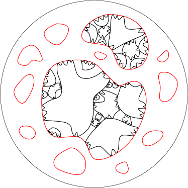
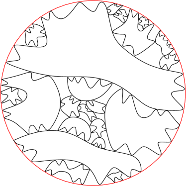
Figure 1.1: Left: We depict the outermost clusters in a double random current with free boundary conditions. The outer boundaries of these clusters are in red (they form a CLE₄). The inner boundaries of the clusters are in black. Right: We depict the unique outermost cluster in a double random current with wired boundary conditions. The inner boundaries of this cluster are in black. For both: In each domain encircled by an inner boundary loop, one has (the scaling limit of) an independent double random current with free boundary conditions. This allows us to iteratively sample the nested interfaces.

For technical reasons that will be discussed later, we focus on simply connected domains $D$ such that $\partial D$ is $C^{1}$.

Theorem 1.2 (Convergence of double random current clusters with wired boundary conditions).

Fix a simply connected domain $D\subsetneq\mathbb{C}$ such that $\partial D$ is $C^{1}$, and let $\eta^{\delta}$ be the nested boundaries contour configuration of ${\mathbf{n}}_{1}^{\delta}+{\mathbf{n}}_{2}^{\delta}$ where $({\mathbf{n}}_{1}^{\delta},{\mathbf{n}}_{2}^{\delta})\sim\mathbf{P}_{(D^{\delta})^{+},(D^{\delta})^{+}}^{\emptyset,\emptyset}$. Then as $\delta\to 0$, $\eta^{\delta}$ converges in distribution to a limit whose law is invariant under all conformal automorphisms of $D$ (see Fig. 1.1 Right). More precisely, we have that

• The inner boundaries of the unique outermost cluster converge to $\mathcal{L}_{-\sqrt{2}\lambda,\sqrt{2}\lambda}$ in $D$.

• If the inner boundary of a cluster converges to $\gamma$, then the outer boundaries of the outermost clusters enclosed by $\gamma$ converge to a CLE₄ in the domain encircled by $\gamma$.

• If the outer boundary of a cluster converges to $\gamma$, then the inner boundaries of this cluster converge to $\mathcal{L}_{-2\lambda,(2\sqrt{2}-2)\lambda}$ in the domain encircled by $\gamma$.

Theorems 1.1 and 1.2 have the following applications.

• The Hausdorff dimension of a double random current cluster in the scaling limit (for both free and wired boundary conditions) is $7/4$ ([SSV]).

• (Difference in log conformal radii) The difference of log conformal radii between two successive loops that encircle the origin in the scaling limit of double random current interfaces is equal to $T_{1}+T_{2}$, where $T_{1}$ is the first time that a standard Brownian motion exits $[-\pi,(\sqrt{2}-1)\pi]$ and $T_{2}$ is the first time that a standard Brownian motion exits $[-\pi,\pi]$ (see [MR3936643, Proposition 20]).

• (Number of clusters) Let $N(\varepsilon)$ be the number of double random current clusters in the unit disk surrounding the origin such that their outer boundaries have a conformal radius w.r.t. the origin at least $\varepsilon$. We will show in Lemma 5.13 that almost surely,

  $$N(\varepsilon)/\log(\varepsilon^{-1})\underset{\varepsilon\to 0}{\longrightarrow}\frac{1}{\sqrt{2}\pi^{2}}.$$

• (Scaling limit of the magnetization in domains) With a little bit of additional work, one may derive from our results the conformal invariance of the $n$-point spin-spin correlations of the critical Ising model already obtained in [CHI] as these correlations are expressed in terms of connectivity properties of ${\mathbf{n}}_{1}^{\delta}+{\mathbf{n}}_{2}^{\delta}$. The additional technicalities would consist in relating the point-to-point connectivity in ${\mathbf{n}}_{1}^{\delta}+{\mathbf{n}}_{2}^{\delta}$ to the probabilities that the $\varepsilon$-neighborhoods of the points are connected. Such reasonings have been implemented repeatedly when proving conformal invariance, and we omit the details here as it would lengthen the paper even more. We still wished to mention this corollary even though the result is already known as our paper mostly uses the convergence of certain fermionic observables to obtain convergence of the nesting field height function to the GFF. Such fermionic observables convergence has been obtained for the Ashkin–Teller model (which is a combination of two interacting Ising models) in [GiuMasTon15] via renormalization arguments using the crucial fact that the observables in question are local observables of the Grassmann representation of the model. Notoriously, the spin-spin correlations are not of this kind, which makes renormalization arguments much more difficult to implement. We believe that the strategy of this paper may be of use to extend the universality results from [GiuMasTon15] to non-local Grassmann observables.

Finally, we remark that Theorems 1.1 and 1.2 are simplified versions of more detailed results (see Theorems 5.1 and 5.3) that we will prove in Section 5. We do not include all details in the introduction in order to facilitate the reading, but let us make some comments on the additional properties that we can obtain:

• The proofs of Theorems 1.1 and 1.2 rely on the coupling of the models with a height function that we will present in the next subsection. In fact, the primal and dual double random currents can be coupled together with the same height function (see Theorem 2.1). Consequently, the limiting interfaces of the primal and dual models are also coupled with the same GFF, so that we fully understand the nesting and intersecting behavior of their limiting interfaces.

• Theorems 1.1 and 1.2 state the convergence of the boundaries of double random current clusters. However, apart from the shape of the clusters, we also have an additional information on whether the current is even or odd on each edge. A hole of a double random current cluster is called odd if it is surrounded by odd currents, and otherwise it is called even. In the discrete, given the shape of the clusters, there is additional randomness to determine the parity of the holes. However, in the continuum limit, as we will show in Theorem 5.1, the parity of each hole in a double random current cluster with free b.c. is a deterministic function of the shape of the cluster.

1.3 Convergence of the nesting field of the double random current to the Gaussian free field

As mentioned above, a central piece in our strategy is a new convergence result dealing with the so-called nesting field of the double random current introduced by two of the authors in [DumLis]. Let $G=(V,E)$ be a generic planar graph. Let ${\mathbf{n}}_{\rm odd}$ be the set of edges that have an odd current in ${\mathbf{n}}$. A nontrivial connected component of the graph $(V,\mathbf{n}_{\rm odd})$ will be called a contour. In particular, each contour $C$ is contained in a unique cluster of $\mathbf{n}$, and each cluster $\mathscr{C}$ is associated to a contour configuration $\mathscr{C}\cap\mathbf{n}_{\rm odd}$. Each contour configuration gives rise to a $\pm 1$ spin configuration on the faces of $G$, where the external unbounded face is assigned spin $+1$, and where the spin changes whenever one crosses an edge of a contour. We call a cluster $\mathscr{C}$ odd around a face $u$ if the spin configuration associated with the contour configuration $\mathscr{C}\cap\mathbf{n}_{\rm odd}$ assigns spin $-1$ to $u$.

For a current ${\mathbf{n}}$, let $\mathfrak{C}({\mathbf{n}})$ be the collection of all clusters of ${\mathbf{n}}$, and let $(\epsilon_{\mathscr{C}})_{\mathscr{C}\in\mathfrak{C}({\mathbf{n}})}$ be i.i.d. random variables equal to $+1$ or $-1$ with probability $1/2$ indexed by $\mathfrak{C}({\mathbf{n}})$. These random variables are called the labels of the clusters. The nesting field with free boundary conditions of a current ${\mathbf{n}}$ on $G$ evaluated at a face $u$ of $G$ is defined by

$$h_{G}(u):=\sum_{\mathscr{C}\in\mathfrak{C}({\mathbf{n}})}\mathbf{1}\{\mathscr{C}\text{ odd around }u\}\epsilon_{\mathscr{C}}.$$ (1.4)

Analogously, the nesting field with wired boundary conditions of a current ${\mathbf{n}}$ on $G^{+}$ evaluated at a face $u$ of $G^{+}$ is defined by

$$h^{+}_{G^{+}}(u):=(1/2-\mathbf{1}\{\mathscr{C}_{\mathfrak{g}}\text{ odd around }u\})\epsilon_{\mathscr{C}_{\mathfrak{g}}}+\sum_{\mathscr{C}\neq\mathscr{C}_{\mathfrak{g}}}\mathbf{1}\{\mathscr{C}\text{ odd around }u\}\epsilon_{\mathscr{C}},$$ (1.5)

where $\mathscr{C}_{\mathfrak{g}}$ is the cluster containing the external vertex $\mathfrak{g}$, and where the sum is taken over all remaining clusters of ${\mathbf{n}}$. Here, whether $\mathscr{C}_{\mathfrak{g}}$ is odd around a face of $G$ or not depends on the embedding of the graph $G^{+}$. However, one can see that the distribution of $h^{+}_{G^{+}}(u)$ is independent of this embedding.

Note that due to the term corresponding to $\mathscr{C}_{\mathfrak{g}}$, the nesting field with wired boundary conditions takes half-integer values, whereas the one with free boundary conditions is integer-valued. Such definition is justified by the next result, and by the joint coupling of $h_{G}$ and $h^{+}_{G^{*}}$ via a dimer model described in Section 2.2.3. We note that the global shift of $1/2$ between $h_{G}$ and $h^{+}_{G^{*}}$ is the same as in the work of Boutilier and de Tilière [BoudeT].

The following is the main result of this part of the argument. We identify the function $h_{D^{\delta}}$ defined on the faces of $D^{\delta}$ with a distribution on $D$ in the following sense: extend $h_{D^{\delta}}$ to all points in $D$ by setting it to be equal to $h_{D^{\delta}}(u)$ at every point strictly inside the face $u$, and 0 on the complement of the faces in $D$. Then, we view $h_{D^{\delta}}$ as a distribution (generalized function) by setting

$$h_{D^{\delta}}(f):=\int_{D}f(x)h_{D^{\delta}}(x)dx,$$

where $f$ is a test function, i.e. a smooth compactly supported function on $D$. We proceed analogously with the field $h^{+}_{(D^{\delta})^{*}}$ and extend it to all points within the faces of $(D^{\delta})^{*}$.

The Gaussian free field (GFF) $h_{D}$ with zero boundary conditions in $D$ is a random distribution such that for every smooth function $f$ with compact support in $D$, we have

$$\mathbb{E}\bigg{[}\bigg{(}\int_{D}f(z)h_{D}(z)dz\bigg{)}^{2}\bigg{]}=\int_{D}\int_{D}f(z_{1})f(z_{2})G_{D}(z_{1},z_{2})dz_{1}dz_{2},$$ (1.6)

where $G_{D}$ is the Green’s function on $D$ with zero boundary conditions satisfying $\Delta G_{D}(x,\cdot)=-\delta_{x}(\cdot)$, where $\delta_{x}$ denotes the Dirac mass at $x$. This normalization means e.g. that for the upper half plane $\mathbb{H}$, we have $G_{\mathbb{H}}(x,y)=\tfrac{1}{2\pi}\log|(x-\bar{y})/(x-y)|$.

Theorem 1.3 (Convergence of the nesting field).

Let $D\subsetneq\mathbb{C}$ be a bounded simply connected Jordan domain and let $D^{\delta}\subsetneq\delta\mathbb{Z}^{2}$ converge to $D$ as $\delta\to 0$ in the Carathéodory sense. Denote by $h_{D^{\delta}}$ the nesting field of the critical double random current model on $D^{\delta}$ with free boundary conditions, and by $h^{+}_{(D^{\delta})^{\dagger}}$ the nesting field of the critical double random current model on the weak dual graph $(D^{\delta})^{\dagger}$ with wired boundary conditions. Then

$$\lim_{\delta\rightarrow 0}h_{D^{\delta}}=\lim_{\delta\rightarrow 0}h^{+}_{(D^{\delta})^{\dagger}}=\frac{1}{\sqrt{\pi}}h_{D},$$

where $h_{D}$ is the GFF in $D$ with zero boundary conditions, and where the convergence is in distribution in the space of generalized functions.

Moreover, $h_{D^{\delta}}$ and $h^{+}_{(D^{\delta})^{\dagger}}$ can be coupled together as one random height function $H_{D^{\delta}}$ defined on the faces of a planar graph $C_{D^{\delta}}$ (whose faces correspond to both the faces of $D^{\delta}$ and $(D^{\delta})^{\dagger}$; see Fig. 2.1) in such a way that

$$\lim_{\delta\rightarrow 0}H_{D^{\delta}}=\frac{1}{\sqrt{\pi}}h_{D}.$$

More properties of the coupling of $h_{D^{\delta}}$ and $h^{+}_{(D^{\delta})^{\dagger}}$ are described in Section 2.1.

Our proof is based on the relationship between the nesting field of double random currents on a graph $G$ and the height function of a dimer model on decorated graphs $G^{d}$ and $C_{G}$ established in [DumLis]. We will first explicitly identify the inverse Kasteleyn matrix associated with these dimer models with the correlators of real-valued Kadanoff–Ceva fermions in the Ising model [KadCev]. This is valid for arbitrary planar weighted graphs, and can also be derived from the bozonization identities of Dubédat [Dub]. For completeness of exposition, we choose to present an alternative derivation that uses arguments similar to those of [DumLis]. Compared to [Dub], rather than using the connection with the six-vertex model, we employ the double random current model. We then express the real-valued observables on general graph in terms of the complex-valued observables of Smirnov [smirnov], Chelkak and Smirnov [CheSmi12] and Hongler and Smirnov [HonSmi]. This is a well-known relation that can be e.g. found in [CCK]. We also state the relevant scaling limit results for the critical observables on the square lattice obtained in [smirnov, CheSmi12, HonSmi].

All in all, we identify the scaling limit of the inverse Kasteleyn matrix on graphs $C_{D^{\delta}}$ as $\delta\to 0$. This is an important ingredient in the computation of the limit of the moments of the height function which is done by modifying an argument of Kenyon [Ken00]. Another crucial and new ingredient is a class of delicate estimates on the critical random current model from [DumLisQia21] that allow us to do two things:

• to identify the boundary conditions of the limiting GFF to be zero boundary conditions;

• to control the behaviour of the increments of the height function between vertices at small distances.

The first item is particularly important as handling boundary conditions directly in the dimer model is notoriously difficult. Here, the identification of the limiting boundary conditions is made possible by the connection with the double random current as well as the main result of [DumLisQia21] stating that large clusters of the double random current with free boundary conditions do not come close to the boundary of the domain (see Theorem 4.10 below). We see this observation and its implication for the nesting field as one of the key innovation of our paper.

We stress the fact that Theorem 1.3 does not follow from the scaling limit results of Kenyon [Ken00, Ken01] as the boundary conditions considered in these papers are related to Temperley’s bijection between dimers and spanning trees [Temp, KPW, KenShe], whereas those considered in this paper correspond to the double Ising model [DumLis, Dub, BoudeT]. Moreover we note that the infinite volume version of Theorem 1.3 was obtained by de Tilière [DeT07]. Finally it can also be shown that the hedgehog domains of Russkikh [Rus] are a special case of our framework, where the boundary of $D^{\delta}$ makes turns at each discrete step.

Organization

The paper is organized as follows. In Section 2 we recall the relationship between different discrete models and derive a connection between the inverse Kasteleyn matrix and complex-valued fermionic observables. While some (but not all) of these results are not completely new, they are scattered around the literature and we therefore review them here. In Section 3 we derive Theorem 1.3. Section 4 presents more preliminaries on the continuum objects. Section 5 is devoted to the identification of the scaling limit of double random currents.

Acknowledgements

We are grateful to Juhan Aru for pointing out a mistake in the previous version of the paper. The first author was supported by the NCCR SwissMap from the FNS. This project has received funding from the European Research Council (ERC) under the European Union’s Horizon 2020 research and innovation program (grant agreement No. 757296). The beginning of the project involved a number of people, including Gourab Ray, Benoit Laslier, and Matan Harel. We thank them for inspiring discussions. The project would not have been possible without the numerous contributions of Aran Raoufi to whom we are very grateful. We thank Pierre Nolin for useful comments on an earlier version of this paper. We thank Wendelin Werner for reading a later version of this paper, and for insightful comments which improved the paper.

2 Preliminaries on discrete models

2.1 A coupling between the primal and dual double random current

In this section we discuss the joint coupling of the double random current on a primal graph and the double random current on the dual graph together with a height function that restricts to both the nesting field of the primal and the dual random current. The coupling constants for the dual model satisfy the Kramers–Wannier duality relation

$$\exp(-2\beta^{*}J^{*}_{e^{*}})=\tanh(\beta J_{e}).$$

We note that if $J_{e}=J^{*}_{e^{*}}=1$ for all $e$, and $\beta=\beta_{c}$, $\beta^{*}=\beta_{c}$ (the critical point is self dual). Properties of this coupling will be used in Section 5 to identify the scaling limit of the boundaries of the double random current clusters. We will provide a proof of this result at the end of Section 2.2.3 using a relation with the dimer model.

Theorem 2.1 (Master coupling).

One can couple the following objects:

1. a double random current model ${\mathbf{n}}$ with free boundary conditions on the primal graph $G=(V,E)$, together with i.i.d. $\pm 1$-valued spins $(\tau_{\mathcal{C}}:\mathcal{C}\in\mathfrak{C}({\mathbf{n}}))$ associated to each cluster of ${\mathbf{n}}$,

2. the dual double random current model ${\mathbf{n}}^{\dagger}$ with wired boundary conditions on the weak dual graph $G^{\dagger}$ (equivalently with free boundary conditions on the full dual graph $G^{*}=(U,E^{*})$) and with the dual coupling constants, together with i.i.d. $\pm 1$-valued spins $(\tau^{\dagger}_{\mathcal{C}}:\mathcal{C}\in\mathfrak{C}({\mathbf{n}}^{\dagger}))$ associated with each cluster of ${\mathbf{n}}^{\dagger}$,

3. a height function $H$ defined on $V\cup U$,

in such a way that the following properties hold:

1. The odd part of ${\mathbf{n}}$ is equal to the collection of interfaces of $\tau^{\dagger}$, and the odd part of ${\mathbf{n}}^{\dagger}$ is equal to the collection of interfaces of $\tau$.

2. For a face $u\in U$ and a vertex $v\in V$ incident on $u$, we have

   $$H(u)-H(v)=\tfrac{1}{2}\tau^{\dagger}_{u}\tau_{v}.$$

   By property (1), each cluster $\mathcal{C}$ of ${\mathbf{n}}$ (resp. a cluster of ${\mathbf{n}}^{\dagger}$ different from the cluster of the ghost vertex $\mathfrak{g}$) can be assigned a well-defined dual spin $\tau^{\dagger}_{\mathcal{C}}$ (resp. $\tau_{\mathcal{C}}$). This is the spin assigned to any face of $G$ (resp. $G^{*}$) incident on $\mathcal{C}$ from the outside. For the cluster of $\mathfrak{g}$ we set this spin to be $+1$.

   With this definition, the height function $H$ restricted to the faces of $G$ (resp. $G^{*}$) has the law of the nesting field of ${\mathbf{n}}$ with free boundary conditions (resp. ${\mathbf{n}}^{\dagger}$ with wired boundary conditions) with labels associated to the clusters as in the definition (1.3) given by

   $$\epsilon_{\mathcal{C}}=\tau_{\mathcal{C}}\tau^{\dagger}_{\mathcal{C}}.$$ (2.1)

3. The configurations ${\mathbf{n}}$ and ${\mathbf{n}}^{\dagger}$ are disjoint in the sense that ${\mathbf{n}}_{e}>0$ implies ${\mathbf{n}}^{\dagger}_{e^{*}}=0$ and ${\mathbf{n}}^{\dagger}_{e^{*}}>0$ implies ${\mathbf{n}}_{e}=0$, where $e^{*}$ is the dual edge of $e$.

Recall that in the definition of the nesting field (1.4), the labels are independent given the current, and one can see that indeed the variables $(\epsilon_{\mathcal{C}})_{\mathcal{C}\in\mathfrak{C}({\mathbf{n}})}$ as defined by (2.1) are independent given ${\mathbf{n}}$ as $\tau^{\dagger}_{\mathcal{C}}$ is a deterministic function of ${\mathbf{n}}$, and $\tau_{\mathcal{C}}$ are independent by definition.

Remark 2.2.

We note that the laws of $\tau$ and $\tau^{\dagger}$ are those of a XOR Ising model and the dual XOR Ising model respectively. However, we will not use this fact in the rest of the article. An extension of this coupling to the Ashkin–Teller model can be found in the works [LisHF, LisAT] that appeared before but were based on the current article. Here we will provide a different proof that uses the associated dimer model representation.

We stress that the fact that the interfaces of $\tau$ and $\tau^{\dagger}$ are disjoint in the sense of Property 3 appears already in the works of Dubédat [Dub], and Boutilier and de Tilière [BoudeT]. However, Property 3 is a stronger statement as it concerns the full double random current, and not only its odd part.

2.2 Mappings between discrete models

In this section we recall the combinatorial equivalences between double random currents, alternating flows and bipartite dimers established in [LisT, DumLis]. We will later use them to derive a version of Dubédat’s bosonization identity [Dub]. An additional black-white symmetry for correlators of monomer insertions is established that is not apparent in [Dub]. The results here are stated for general Ising models on arbitrary planar graphs $G=(V,E)$ and with arbitrary coupling constants $(J_{e})_{e\in E}$. We focus on the free boundary conditions case and the wired boundary conditions can be treated analogously, replacing $G$ with $G^{+}$. We will actually mostly consider wired boundary conditions on the dual graph $G^{*}$ which one can think of as $(G^{\dagger})^{+}$, where $G^{\dagger}$ is the weak dual of $G$ whose vertex set does not contain the unbounded faces of $G$.

We start by describing the relevant decorated graphs: the double random current model on a graph $G$ will be related to the alternating flow model on a directed graph $\vec{G}$, and the dimer model on two bipartite graphs $G^{d}$ and $C_{G}$. All these graphs are weighted, and their local structure together with the corresponding edge weights are shown in Fig. 2.1. We now describe their construction in detail.

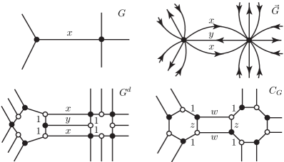
Figure 2.1: One can construct the graphs $\vec{G}$, $G^{d}$ and $C_{G}$ locally around each vertex of $G$. The weights satisfy $y=\tfrac{2x}{1-x^{2}}$, $w=\tfrac{2x}{1+x^{2}}$, $z=\tfrac{1-x^{2}}{1+x^{2}}$. Here $x=x_{e}$ is the high-temperature weight equal to $\tanh(\beta J_{e}$). The edges carrying weight $1$ in $G^{d}$ (resp. in $C_{G}$) are called short (resp. roads), and the remaining edges are called long (resp. streets).

Given $G$, $\vec{G}$ is obtained by replacing each edge $e$ of $G$ by three parallel directed edges $e_{s1}$, $e_{m}$, $e_{s2}$ such that the orientation of the side (or outer) edges $e_{s1}$ and $e_{s2}$ is opposite to the orientation of the middle edge $e_{m}$. The orientation of the middle edge can be chosen arbitrarily.

To obtain $G^{d}$ from $\vec{G}$, we replace each vertex $v$ of $\vec{G}$ by a cycle of vertices of even length which is given by the number of times the orientation of edges in $\vec{G}$ incident on $v$ changes when going around $v$. We colour the new vertices black if the corresponding edges are incoming into $v$ and white otherwise. We then connect the white vertices in a cycle corresponding to $v$ with the appropriate black vertices in a cycle corresponding to $v^{\prime}$, where $v$ and $v^{\prime}$ are adjacent in $\vec{G}$. We call long all the edges of $G^{d}$ that correspond to an edge of $\vec{G}$, and short the remaining edges connecting the vertices in the cycles.

The last graph $C_{G}$ can be constructed directly from $G$ by replacing each edge of $G$ by a quadrangle of edges, and then connecting two quadrangles by an edge if the corresponding edges of $G$ share a vertex and are incident to the same face (see Fig. 2.1). Following [Dub], we call streets the edges in the quadrangles and roads those connecting the quadrangles (which represent cities).

We note that the set of faces $U$ (resp. vertices $V$) of $G$ naturally embeds into the set of faces of $\vec{G}$, $G^{d}$ and $C_{G}$ (resp. $G^{d}$ and $C_{G}$). We therefore think of $U$ and $V$ as subsets of the set of faces of the respective decorated graphs (e.g., when we talk about equality in distribution of the height function on $C_{G}$ and the nesting field on $G$).

In the remainder of this section we describe the mappings between the different models in the following order: In Section 2.2.1, Alternating flows on $\vec{G}$ are mapped by an application $\theta$ to the image by a map $\vartheta$ of double random currents on $G$. In Section 2.2.2, dimers on $G^{d}$ are mapped by an application $\pi$ to alternating flows on $\vec{G}$. In Section 2.2.3, dimers on $G^{d}$ are mapped to dimers on $C_{G}$. The corresponding statements for wired boundary conditions can be recovered by replacing $G$ with $G^{+}$.

The first two maps yield relations between configurations of the associated models, and the last map is described as a sequence of local transformations (urban renewals) of the graphs $C_{G}$ or $G^{d}$ that does not change the distribution of the height function on a certain subset of the faces of these two graphs.

We first describe relations on the level of distributions on configurations where no sources or disorders are imposed. Later on (in Section 2.3) we increase the complexity by introducing sources.

2.2.1 Double random currents on $G$ and alternating flows on $\vec{G}$

A sourceless alternating flow $F$ is a set of edges of the directed graph $\vec{G}$ satisfying the alternating condition, i.e., for each vertex $v$, the edges in $F$ that are incident to $v$ alternate between being oriented towards and away from $v$ when going around $v$ (see Fig. 2.2). In particular, the same number of edges enters and leaves $v$. We denote the set of sourceless alternating flows on $\vec{G}$ by $\mathcal{F}^{\emptyset}$, and following [LisT], we define a probability measure on $\mathcal{F}^{\emptyset}$ by the formula, for every $F\in\mathcal{F}^{\emptyset}$,

$$\mathbf{P}^{\emptyset}_{\textnormal{flow}}(F):=\frac{1}{Z^{\emptyset}_{\textnormal{flow}}}\textnormal{w}_{\textnormal{flow}}(F),$$ (2.2)

where $Z^{\emptyset}_{\textnormal{flow}}$ is the partition function of sourceless flows and, if $V(F)$ denotes the set of vertices in the graph $(V,F)$ that have at least one incident edge,

$$\textnormal{w}_{\textnormal{flow}}(F):=2^{|V|-|V(F)|}\prod_{e\in F}x_{e},$$ (2.3)

with the weights $x_{\vec{e}}$ as in Fig. 2.1. We also define the height function of a flow $F$ to be a function $h=h_{F}$ defined on the faces of $\vec{G}$ in the following way:

• $h(u_{0})=0$ for the unbounded face $u_{0}$,

• for every other face $u$, choose a path $\gamma$ connecting $u_{0}$ and $u$, and define $h(u)$ to be total flux of $F$ through $\gamma$, i.e., the number of edges in $F$ crossing $\gamma$ from left to right minus the number of edges crossing $\gamma$ from right to left.

The function $h$ is well defined, i.e., independent of the choice of $\gamma$, since at each $v\in V$, the same number of edges of $F$ enters and leaves $v$ (and so the total flux of $F$ through any closed path of faces is zero).

We are ready to state the correspondence between double random currents and alternating flows. Consider the map $\vartheta$ from $\boldsymbol{\Omega}^{B}$ to the set $\Omega^{B}$ of pairs $(E_{\rm odd},E_{\rm even})$ of subsets of $E$ with $E_{\rm odd}$ of even degree at every vertex in $V\setminus B$, and odd degree at every vertex in $B$, obtained as follows:

$$\vartheta({\mathbf{n}}):=({\mathbf{n}}_{\rm odd},{\mathbf{n}}_{\rm even})\text{ where }\begin{array}[]{l}\text{${\mathbf{n}}_{\rm odd}$ is the set of edges $e$ with ${\mathbf{n}}_{e}$ odd,}\\ \text{${\mathbf{n}}_{\rm even}$ is the set of edges with ${\mathbf{n}}_{e}$ even and strictly positive.}\end{array}$$

In what follows we will often identify a current ${\mathbf{n}}$ with the pair $({\mathbf{n}}_{\rm odd},{\mathbf{n}}_{\rm even})$ as it carries all the relevant information for our considerations.

Also define a map $\theta:\mathcal{F}^{\emptyset}\to\Omega^{\emptyset}$ as follows. For every $F\in\mathcal{F}^{\emptyset}$ and every $e\in E$, consider the number of corresponding directed edges $e_{m}$, $e_{s1}$, $e_{s2}$ that are present in $F$. Let $\mathbf{n}_{\rm odd}\subseteq E$ be the set with one or three such present edges, and $\mathbf{n}_{\rm even}\subseteq E$ the set with exactly two such edges, and set

$$\theta(F):=(\mathbf{n}_{\rm odd},\mathbf{n}_{\rm even}).$$

Denote by $\theta_{*}\mathbf{P}_{\textnormal{flow}}^{\emptyset}$ the pushforward measure on $\Omega^{\emptyset}$. The following result was proved in [DumLis, LisT].

Lemma 2.3 ([DumLis]).

We have $\theta_{*}\mathbf{P}_{\textnormal{flow}}^{\emptyset}=\vartheta_{*}\mathbf{P}_{\textnormal{dcur}}^{\emptyset}$. Moreover, under this identification the restrictions to $U$ of the nesting field of double random currents and the height function of the alternating flows have the same distribution.

Proof.

This is a consequence of the fact that the total weight of all alternating flows corresponding to a cluster in the double random current, and whose outer boundary is oriented clockwise is the same as those oriented counterclockwise (see also the proof of Lemma 2.9). This corresponds to the fact that the nesting field is defined using symmetric coin flip random variables $\epsilon_{\mathscr{C}}$. Moreover, the sum of these two weights is the same as the weight of the cluster in the double random current model. The details are provided in [DumLis]. ∎

2.2.2 Alternating flows on $\vec{G}$ and dimers on $G^{d}$

Figure 2.2: Left: A configuration $\vartheta({\mathbf{n}})=({\mathbf{n}}_{\rm odd},{\mathbf{n}}_{\rm even})$ on a piece of the hexagonal lattice $G$. The blue edges represent ${\mathbf{n}}_{\rm odd}$ and the red edges represent ${\mathbf{n}}_{\rm even}$. The blue and red edges together form one cluster $\mathscr{C}$. Middle: Two alternating flow configurations on $\vec{G}$ mapped to $\vartheta({\mathbf{n}})$ under $\theta$. The two clusters have opposite orientations of the outer boundary. Depending on this orientation the height function either increases or decreases by one when going from the outside to the inside of the lower hexagon. This corresponds to two different outcomes for the label $\epsilon_{\mathscr{C}}$ in the definition of the nesting field (1.4). Right: Two dimer configurations on $G^{d}$ that map to the corresponding alternating flows under $\pi$. Note that the parity of the height function on $G^{d}$ restricted to the vertices of $\mathscr{C}$ and shifted by $1/2$ changes whenever the sign of $\epsilon_{\mathscr{C}}$ changes. This can be seen from the placement of the dimers on the short edges. This property is used in the proof of Theorem 2.1. On the other hand the parity of the height function on the faces of $G$ is independent of $\epsilon_{\mathscr{C}}$.
We also note that both $\pi$ and $\theta$ are many-to-one maps.

Consider a weighted graph $G$. Recall that a dimer cover (or perfect matching) $M$ of $G$ is a subset of edges such that every vertex of the graph is incident to exactly one edge of $M$. We write $\mathcal{M}(G)$ for the set of all dimer covers of $G$. The dimer model is a probability measure on $\mathcal{M}(G)$ which assign a probability to a dimer cover that is proportional to the product of the edge-weights over the dimer cover.

To each dimer cover $M$ on a bipartite planar finite graph $G$ (implicitly colored in black and white in a bipartite fashion, one can associate a 1-form $f_{M}$ (i.e. a function defined on directed edges which is antisymmetric under a change of orientation) satisfying $f_{M}((v,v^{\prime}))=-f_{M}((v^{\prime},v))=1$ if $\{v,v^{\prime}\}\in M$ and $v$ is white, and $f_{M}((v,v^{\prime}))=0$ otherwise. For a 1-form $f$ and a vertex $v$, let $df(v)=\sum_{v^{\prime}\sim v}f((v,v^{\prime}))$ be the divergence of $f$ at $v$. Note that for a dimer cover $M$, $df_{M}(v)=1$ if $v$ is white, and $df_{M}(v)=-1$ if $v$ is black. Fixing a reference 1-form $f_{0}$ with the same divergence, we define the height function $h=h_{M}$ by

• $h(u_{0})=0$ for the unbounded face $u_{0}$,

• for every other face $u$, choose a dual path $\gamma$ connecting $u_{0}$ and $u$, and define $h(u)$ to be the total flux of $f_{M}-f_{0}$ through $\gamma$, i.e., the sum of values of $f_{M}-f_{0}$ over the edges crossing $\gamma$ from left to right.

The height function is well defined, i.e. independent of the choice of $\gamma$, since $f_{M}-f_{0}$ is a divergence-free flow, i.e. $d(f_{M}-f_{0})=0$.

We will write $\mathbf{P}^{\emptyset}_{G^{d}}$ for the dimer model measure on $G^{d}$ with weights as in Fig. 2.1. We also fix a reference 1-form $f_{0}$ on $G^{d}$ given by

• $f_{0}((w,b))=-f_{0}((b,w))=1/2$ if $\{w,b\}$ is a short edge and $w$ is white,

• $f_{0}((w,b))=f_{0}((b,w))=0$ if $\{w,b\}$ is a long edge.

We now describe a straightforward map $\pi$ from the dimer covers on $G^{d}$ to alternating flows on $\vec{G}$ that preserves the law of the height function. We note that one could carry out the same discussion and make a connection with double random currents directly, without introducing alternating flows. However, we find the language of alternating flows particularly convenient to express some of the crucial steps discussed later on (especially Lemmata 2.9 and 2.10). To this end, to each matching $M\in\mathcal{M}(G^{d})$, associate a flow $\pi(M)\in\mathcal{F}^{\emptyset}$ by replacing each long edge in $M$ by the corresponding directed edge in $\vec{G}$. One can check that this always produces an alternating flow. Indeed, assuming otherwise, there would be two consecutive edges in $F(M)$ of the same orientation, and therefore the path of short edges connecting them in a cycle would be of odd length and therefore could not have a dimer cover, which is a contradiction. Let $\pi_{*}\mathbf{P}_{G^{d}}^{\emptyset}$ be the pushforward measure on $\mathcal{F}^{\emptyset}$ under the map $\pi$.

Lemma 2.4 ([DumLis]).

We have $\pi_{*}\mathbf{P}_{G^{d}}^{\emptyset}=\mathbf{P}_{\textnormal{flow}}^{\emptyset}$. Moreover, under this identification, the restriction to $U$ of the height functions of the dimer model and alternating flows have the same distribution.

Proof.

This is a consequence of the fact that the reference 1-form vanishes on long edges, and hence its contribution to the increment of the height function across a long edge of $G^{d}$ is equal to zero, and the fact that the weights of the edges of $\vec{G}$ and the long edges of $G^{d}$ are the same. Moreover, if a vertex $v$ has zero flow through it, i.e, $v\in V\setminus V(F)$, then there are exactly $2$ dimer covers of the cycle of short edges of $G^{d}$ corresponding to $v$. Since both of these covers have total edge-weight $1$, this accounts for the factor $2^{|V|-|V(F)|}$ in (2.3). ∎

2.2.3 Dimers on $G^{d}$ and on $C_{G}$

We will write $\mathbf{P}^{\emptyset}_{C_{G}}$ for the dimer model measure on $C_{G}$ with weights as in Fig. 2.1. The dimer models on $G^{d}$ and $(G^{*})^{d}$ are closely related to the dimer model on $C_{G}$ (as was described in [DumLis]) using standard dimer model transformations called the vertex splitting and urban renewal, see Fig. 2.3.

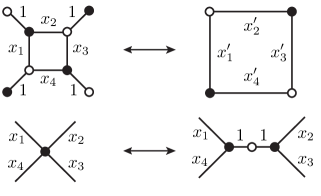
Figure 2.3: Urban renewal and vertex splitting are transformations of weighted graphs preserving the distribution of dimers and the height function outside the modified region. The weights in urban renewal satisfy $x_{1}^{\prime}=\tfrac{x_{3}}{x_{1}x_{3}+x_{2}x_{4}}$, $x_{2}^{\prime}=\tfrac{x_{4}}{x_{1}x_{3}+x_{2}x_{4}}$, $x_{3}^{\prime}=\tfrac{x_{1}}{x_{1}x_{3}+x_{2}x_{4}}$, $x_{4}^{\prime}=\tfrac{x_{2}}{x_{1}x_{3}+x_{2}x_{4}}$.

Lemma 2.5 ([DumLis]).

One can transform $G^{d}$ and $(G^{*})^{d}$ to $C_{G}$ (and the other way around) using urban renewals and vertex splittings.

Proof.

We will describe how to transform $G^{d}$ to $C_{G}$. The second part follows since $C_{G}$ is symmetric with respect to $G$ and $G^{*}$.

To this end, note that to each edge $e$ in $G$, there corresponds one quadrilateral in $C_{G}$, and two quadrilaterals in $G^{d}$. Given $e$, choose for the internal quadrilateral of urban renewal the quadrilateral in $G^{d}$ with the opposite colors of vertices. Then, split each vertex that the chosen quadrilateral shares with a quadrilateral corresponding to a different edge of $G$. In this way we find ourselves in the situation from the upper left panel in Fig. 2.3. After performing urban renewal and collapsing the doubled edge, we are left with one quadrilateral as desired. One can check that the weights that we obtain match those from Fig. 2.1. We then repeat the procedure for every edge of $G$. The resulting graph is $C_{G}$. ∎

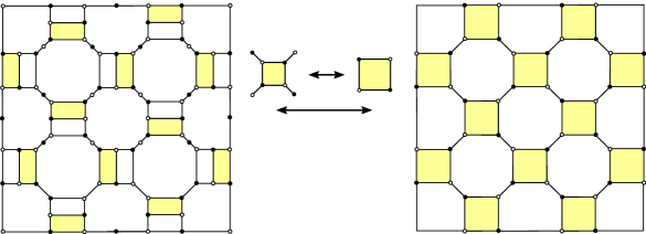
Figure 2.4: An example of the correspondence between dimer models on $G^{d}$ and $C_{G}$. The yellow quadrilaterals are transformed using urban renewal moves. The underlying graph $G$ is a $3\times 3$ piece of the square lattice.

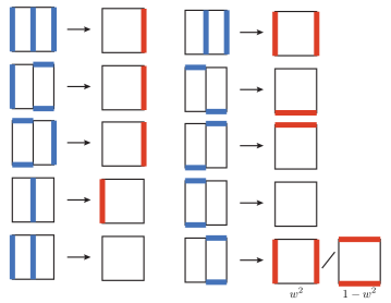
Figure 2.5: The figure shows the measure preserving mapping of local configurations on $G^{d}$ (corresponding to a single edge $e$ of $G$) to local configurations on the streets of $C_{G}$ under urban renewal performed on the left-hand side quadrilateral in $G^{d}$. The last case involves additional random choice between two possible configurations. These choices are independent for local configurations corresponding to different edges of $G$ and the probabilities are as in the figure with $w=2x/(1+x^{2})$.

A choice of quadrilaterals where urban renewals are applied for a rectangular piece of the square lattice is depicted in Fig. 2.4. In this way, the XOR-Ising model on the square lattice is related to a (weighted) dimer model on the square-octagon lattice. In Fig. 2.5, we illustrate the behaviour of local dimer configurations under one urban renewal performed in the construction described in the lemma above.

As the reference 1-form for the dimer model on $C_{G}$ we choose the canonical one given by

$$f_{0}((w,b))=-f_{0}((b,w))=\mathbf{P}^{\emptyset}_{C_{G}}(\{w,b\}\in M),$$ (2.4)

where $w$ is a white vertex. Note that this makes the height function centered as all its increments become centered by definition. This is the same 1-form as used in [BoudeT] on the infinite square-octagon lattice $C_{\mathbb{Z}^{2}}$. In [KenLaplacian], two crucial properties of $f_{0}$ were established when $G$ is an infinite isoradial graph and the Ising model on $G$ is critical. In the next lemma we show that both of these properties hold for arbitrary Ising weights on general finite planar graphs.

Lemma 2.6.

We have

• $\mathbf{P}^{\emptyset}_{C_{G}}(e\in M)=1/2$, if $e$ is a road, i.e., $e$ corresponds to a corner of $G$,

• $\mathbf{P}^{\emptyset}_{C_{G}}(e\in M)=\mathbf{P}^{\emptyset}_{C_{G}}(e^{\prime}\in M)$, if $e$ and $e^{\prime}$ are two parallel streets corresponding to the same edge of $G$ (or of the dual $G^{*}$).

In the proof, which is postponed to the end of Section 2.3, we actually compute the probability from the second item in terms of the underlying Ising measure. However, the exact value will not be important for our considerations. We note that the first bullet of the lemma above is the reason why the nesting field with free boundary conditions on $G$ is defined to be integer-valued and the one with wired boundary conditions on $G^{*}$ to be half-integer valued.

A crucial observation now is that the height function on the faces of $G^{d}$ corresponding to the faces and vertices of $G$ is not modified by vertex splitting and urban renewal. This follows from basic properties of these transformations, and the fact that the reference 1-form on the short edges of $G^{d}$ is the same as the one on the roads of $C_{G}$ (by the first item of the lemma above). Indeed, one can compute the height function on the faces of $G^{d}$ and $C^{G}$ corresponding to the faces and vertices of $G$ using only increments across short edges and roads respectively. This means that the resulting height function on these faces of $C_{G}$ has the same distribution as the one on $G^{d}$. Since $C_{G}$ plays the same role with respect to $G^{*}$ as to $G$, we immediately get the following corollary.

Corollary 2.7.

The height function on $C_{G}$ restricted to the faces and vertices of $G$ is distributed as the the height functions on $G^{d}$ and $(G^{*})^{d}$ restricted to the faces and vertices of $G$. In particular, the height function on $C_{G}$ restricted to the faces of $G$ has the law of the nesting field of the double random current with free boundary conditions on $G$, and restricted to the vertices of $G$ has the law of the nesting field of the double random current with wired boundary conditions on $G^{\dagger}$ (or free boundary conditions on $G^{*}$).

This observation is at the heart of the proof of the master coupling for double random currents and the XOR-Ising model from Theorem 2.1. However, one has to be careful since there is loss of information between the dimer model on $G^{d}$ and the one on $C_{G}$. Indeed, a dimer configuration on $C_{G}$ does not contain information on where the even nonzero values of the double random current are. To recover it, one needs to add additional randomness in the form of independent coin flips for each edge of $G$ with a proper success probability.

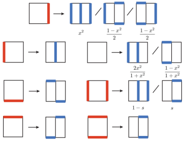
Figure 2.6: The reverse mapping to that in Fig. 2.5. Again, urban renewal is performed on the left-hand side quadrangle of the local configuration on $G^{d}$. Whenever there is ambiguity, we use additional randomness which is independent for each local configuration and with probabilities as in the figure with $s=\frac{2(1-x^{2})}{3+x^{4}}$. These probabilities are simply obtained from Fig. 2.5 using the definitions of the weights in both dimer models on $C_{G}$ and $G^{d}$ and elementary conditional probability computations.

Proof of Theorem 2.1.

We will use a procedure reverse to that from the proof of Lemma 2.5. This procedure induces a measure preserving mapping between local configurations on $C_{G}$ and $G^{d}$, see Fig. 2.7, where in certain cases additional randomness is used to decide on the exact configuration on $G^{d}$.

As mentioned, the graph $C_{G}$ plays a symmetric role with respect to $G$ and $G^{*}$. Hence, taking the Kramers–Wannier dual parameters $x_{e}^{*}={(1-x_{e})}/{(1+x_{e})}$ and rotating the local configuration on $C_{G}$ by $\pi/2$, one can use the same mapping from Fig. 2.7 to generate local dimer configurations on $({G^{*}})^{d}$ that will correspond to dual random current configurations. Recall that part of our aim is to couple the double random current on $G$ with its dual on $G^{*}$ so that no edge and its dual are open at the same time. The idea is to first sample a dimer configuration on $C_{G}$, and then using the rules from Fig. 2.7 choose, possibly introducing additional randomness, the dimer configurations on both $G^{d}$ and $(G^{*})^{d}$. The desired property of the coupling will follow from the way we use the additional randomness for $G^{d}$ and $(G^{*})^{d}$.

We now explain this in more detail. In the coupling between double random currents and dimers on $G^{d}$, an edge in the current is closed (or has value zero) if and only if there is no long edge present in the corresponding local dimer configuration. From Fig. 2.7, we see that the only possibility to have nonzero values of double currents for both a primal edge $e$ and its dual $e^{*}$ is when the quadrangle in $C_{G}$ that corresponds to both $e$ and $e^{*}$ has no dimer in the dimer cover. In that case we have a probability of ${2x_{e}^{2}}/({1+x_{e}^{2}})$ to get a non-zero (and even) value of the primal double current and a probability of ${2{(x_{e}^{*})}^{2}}/{(1+{(x_{e}^{*})}^{2})}$ to get a non-zero (and even) value of the dual double current. However, since these choices are independent of the possible choices for other local configurations, and since

$$\frac{2x_{e}^{2}}{1+x_{e}^{2}}+\frac{2{(x_{e}^{*})}^{2}}{1+{(x_{e}^{*})}^{2}}=1-\frac{2x_{e}(1-x_{e})}{1+x_{e}^{2}}<1$$

we can couple the results so that the primal and dual currents are never both open (nonzero) at $e$. Together establishes Property 3 from the statement of the theorem.

We now focus on Property 1. Note that the spins $\tau^{\dagger}$ defined by the interfaces of odd current in ${\mathbf{n}}$ satisfy

$$\tau^{\dagger}_{u}=(-1)^{H(u)}$$ (2.5)

for $u\in U$, where $H$ is the height function on $C_{G}$. By Corollary 2.7 we already know that $H$ restricted to $U$ has the law of the height function on $(G^{*})^{d}$ restricted to $U$. From the relationship between the double random current ${\mathbf{n}}^{\dagger}$ on $G^{*}$ and the alternating flow model on $\vec{G}^{*}$, one can see that the parity of this height function at a face $u$ changes with the change of the orientation of the outer boundary of the cluster of ${\mathbf{n}}^{\dagger}$ containing $u$ (see Fig. 2.2 for a dual example). Therefore $(-1)^{H(u)}$ is distributed as an independent assignment of a sign to each cluster of ${\mathbf{n}}^{\dagger}$. This yields Property 1. A dual argument for

$$\tau_{v}=i(-1)^{H(v)}$$ (2.6)

with $v\in V$, and $i$ the imaginary unit, yields the dual correspondence. Here, the factor $i$ appears due to the fact that the height function takes half-integer values on $V$.

Finally, (2.5) and (2.6) together imply Property 2. ∎

We leave it to the interested reader to check that the resulting coupling of the primal and dual double random current model is the same as the one described in [LisHF] (where no connection with the dimer model is used).

Figure 2.7: The reverse mapping to that in Fig. 2.5. Again, urban renewal is performed on the left-hand side quadrangle of the local configuration on $G^{d}$. Whenever there is ambiguity, we use additional randomness which is independent for each local configuration and with probabilities as in the figure with $s=\frac{2(1-x^{2})}{3+x^{4}}$. These probabilities are simply obtained from Fig. 2.5 using the definitions of the weights in both dimer models on $C_{G}$ and $G^{d}$ and elementary conditional probability computations.

2.3 Disorder and source insertions

It will be important for our analysis to introduce the so-called sources in dimers, alternating flows, and double random currents, and to see how they relate to order-disorder variables in the Ising model.

A corner $c=(u,v)$ of a planar graph $G$ is a pair composed of a face $u=u(c)$ (also seen as a vertex of the dual graph) and a vertex $v=v(c)$ bordering $u$. One can visualize corners as segments from the center of the face $u$ to the vertex $v$ (see Fig. 2.8). In this section we discuss correlations of disorder insertions, by which we mean modifications of the state space of the appropriate model that are localized at the corners of $G$, and describe their mutual relationships. In what follows, consider two corners $c_{i}$ and $c_{j}$, and a simple dual path $\gamma$ connecting $u(c_{i})$ to $u(c_{j})$. For a collection of edges $H$ of $G$, $\vec{G}$, $G^{d}$ or $C_{G}$, we define $\textnormal{sgn}_{\gamma}(H)=-1$ if the number of edges in $H$ crossed by $\gamma$ is odd and $\textnormal{sgn}_{\gamma}(H)=1$ otherwise.

In the following subsections we introduce correlation functions of corner insertions in the relevant models and relate them to each other.

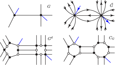
Figure 2.8: Corner insertions in the relevant models can be realized by considering additional edges connecting a vertex and a neighbouring face.

2.3.1 Kadanoff–Ceva fermions via double random currents

The two-point correlation function of Kadanoff–Ceva fermions is defined by

$$\langle\chi_{c_{i}}\chi_{c_{j}}\rangle:=\frac{1}{Z^{\emptyset}_{\text{hT}}}\sum_{\eta\in\mathcal{E}^{\{v(c_{i}),v(c_{j})\}}}\textnormal{sgn}_{\gamma}(\eta)\prod_{e\in\eta}x_{e},$$ (2.7)

where $Z^{\emptyset}_{\text{hT}}:=\sum_{\eta\in\mathcal{E}^{\emptyset}}\prod_{e\in\eta}x_{e}$. Here, $\mathcal{E}^{\emptyset}$ is the collection of sets of edges $\eta\subseteq E$ such that each vertex in the graph $(V,\eta)$ has even degree, and $\mathcal{E}^{\{v(c_{i}),v(c_{j})\}}$ is the collection of sets of edges such that each vertex has even degree except for $v(c_{i})$ and $v(c_{j})$ that have odd degree. Note that the sign of this correlator depends (in this notation, implicitly) on the choice of $\gamma$. However, its amplitude depends only on the corners $c_{i}$ and $c_{j}$.

The next lemma was proved in [ADTW, Lemma 6.3]. It expresses Kadanoff–Ceva correlators in terms of double currents for which $u(c_{i})$ is connected to $u(c_{j})$ in the dual configuration. Below, for $({\mathbf{n}}_{\rm odd},{\mathbf{n}}_{\rm even})\in\Omega^{B}$, let

$$\textnormal{w}_{\textnormal{dcur}}({\mathbf{n}}_{\rm odd},{\mathbf{n}}_{\rm even}):=\sum_{{\mathbf{n}}\in\boldsymbol{\Omega}^{B}:\vartheta({\mathbf{n}})=({\mathbf{n}}_{\rm odd},{\mathbf{n}}_{\rm even})}\textnormal{w}({\mathbf{n}}).$$

For a current ${\mathbf{n}}$, recall the definition of ${\mathbf{n}}^{*}$ from Section 4.2 and for two faces $u$ and $u^{\prime}$, let $u\xleftrightarrow{\mathbf{n}^{*}}u^{\prime}$ mean that $u$ is connected to $u^{\prime}$ in $\mathbf{n}^{*}$, i.e., that $u$ and $u^{\prime}$ belong to the same connected component of the graph $(U,\mathbf{n}^{*})$. We stress the fact that the identity below involves the weight $\textnormal{w}_{\textnormal{dcur}}$ and not the single current weight w.

Lemma 2.8 (fermions via double currents [ADTW]).

We have

$$\langle\chi_{c_{i}}\chi_{c_{j}}\rangle=\frac{1}{Z^{\emptyset}_{\textnormal{dcur}}}\sum_{({\mathbf{n}}_{\rm odd},{\mathbf{n}}_{\rm even})\in\Omega^{\{v(c_{i}),v(c_{j})\}}}\textnormal{sgn}_{\gamma}(\mathbf{n}_{\textnormal{odd}})\textnormal{w}_{\textnormal{dcur}}({\mathbf{n}}_{\rm odd},{\mathbf{n}}_{\rm even})\mathbf{1}\{u(c_{i})\xleftrightarrow{\mathbf{n}^{*}}u(c_{j})\}.$$

2.3.2 Sink and source insertions in alternating flows

Consider the graph $\vec{G}$ with two additional directed edges $c_{i}=(u(c_{i}),v(c_{i}))$ and $-c_{j}=(v(c_{j}),u(c_{j}))$, and let $\mathcal{F}^{c_{i},-c_{j}}$ be the set of alternating flows on this graph that contain both $c_{i}$ and $-c_{j}$. By an alternating flow here we mean a subset of edges of the extended graph that satisfies the alternating condition at every vertex of $\vec{G}$. The weights of $c_{i}$ and $-c_{j}$ are set to $1$. With $\gamma$ defined as above, introduce

$$Z_{\textnormal{flow}}^{\gamma}(c_{i},-c_{j}):=\sum_{F\in\mathcal{F}^{c_{i},-c_{j}}}\textnormal{sgn}_{\gamma}(F)\textnormal{w}_{\textnormal{flow}}(F).$$

Here, $c_{i}$ plays the role of the source and $-c_{j}$ is the sink of the flow $F$.

Recall that $\theta:\mathcal{F}^{\emptyset}\rightarrow\Omega^{\emptyset}$ is the measure preserving map sending sourceless alternating flows on $\vec{G}$ to images by $\vartheta$ of sourceless double current configurations on $G$. With a slight abuse of notation, we also write $\theta$ for the analogous map from $\mathcal{F}^{c_{i},-c_{j}}$ to the image by $\vartheta$ of the set $\Omega^{\{v(c_{i}),v(c_{j})\}}$ of currents on $G$ with sources at $v(c_{i})$ and $v(c_{j})$ (for currents there is no distinction between sources and sinks).

The next lemma is closely related to [LisT, Theorem 4.1].

Lemma 2.9 (Symmetry between sinks and sources).

We have

$$Z_{\textnormal{flow}}^{\gamma}(c_{i},-c_{j})=Z_{\textnormal{flow}}^{\gamma}(c_{j},-c_{i}).$$

Proof.

Note that the flow’s weights on $\vec{G}$ are invariant under the reversal of direction of the flow, i.e., the weights of the three directed edges $e_{s1},e_{m},e_{s2}$ of $\vec{G}$ corresponding to a single edge $e$ of $G$ satisfy $x_{e_{s1}}+x_{e_{s2}}+x_{e_{s1}}x_{e_{s2}}x_{e_{m}}=x_{e_{m}}$ by construction. Hence, for a fixed $({\mathbf{n}}_{\rm odd},{\mathbf{n}}_{\rm even})\in\Omega^{\{v(c_{i}),v(c_{j})\}}$, we have

$$\sum_{F\in\mathcal{F}^{c_{i},-c_{j}}:\ \theta(F)=({\mathbf{n}}_{\rm odd},{\mathbf{n}}_{\rm even})}\textnormal{w}_{\textnormal{flow}}(F)=\sum_{F\in\mathcal{F}^{c_{j},-c_{i}}:\ \theta(F)=({\mathbf{n}}_{\rm odd},{\mathbf{n}}_{\rm even})}\textnormal{w}_{\textnormal{flow}}(F).$$

We finish the proof by summing both sides of this identity over $({\mathbf{n}}_{\rm odd},{\mathbf{n}}_{\rm even})\in\Omega^{\{v(c_{i}),v(c_{j})\}}$, and using the fact that $\textnormal{sgn}_{\gamma}(F)$ depends only on $\theta(F)$. ∎

The next result is a direct analog of Lemma 2.8 with an additional factor of $1/2$ that corresponds to the fact that the connected component of the flow that connects $c_{i}$ to $-c_{j}$ has a fixed orientation.

Lemma 2.10 (Dual connection in alternating flows).

We have

$$\theta(\mathcal{F}^{c_{i},-c_{j}})=\{({\mathbf{n}}_{\rm odd},{\mathbf{n}}_{\rm even})\in\Omega^{\{v(c_{i}),v(c_{j})\}}:u(c_{i})\xleftrightarrow{\mathbf{n}^{*}}u(c_{j})\},$$

and moreover

$$Z_{\textnormal{flow}}^{\gamma}(c_{i},-c_{j})=\tfrac{1}{2}\sum_{({\mathbf{n}}_{\rm odd},{\mathbf{n}}_{\rm even})\in\Omega^{\{v(u_{i}),v(c_{j})\}}}\textnormal{sgn}_{\gamma}(\mathbf{n}_{\textnormal{odd}})\textnormal{w}_{\textnormal{dcurr}}({\mathbf{n}}_{\rm odd},{\mathbf{n}}_{\rm even})\mathbf{1}\{u(c_{i})\xleftrightarrow{\mathbf{n}^{*}}u(c_{j})\}.$$

Proof.

We first argue that for each $({\mathbf{n}}_{\rm odd},{\mathbf{n}}_{\rm even})=\theta(F)$ with $F\in\mathcal{F}^{c_{i},-c_{j}}$, we have that $u(c_{i})\xleftrightarrow{\mathbf{n}^{*}}u(c_{j})$. This follows from topological arguments and the alternating condition for flows. Indeed, assume by contradiction that there is a cycle of edges in $F$ separating $u(c_{i})$ from $u(c_{j})$, and choose the innermost such cycle surrounding $u(c_{i})$. Consider the vertex $v$ of this cycle that is first visited on a path from $c_{i}$ to $-c_{j}$. The alternating condition implies that the edges of the cycle on both sides of $v$ should be oriented away from $v$. Following that orientation around the cycle, we must arrive at another vertex $v^{\prime}$ of the cycle where both incident edges are oriented towards $v^{\prime}$. That is in contradiction with the alternating condition and the fact that the cycle is minimal. The fact that the image of the map is $\{u(c_{i})\xleftrightarrow{\mathbf{n}^{*}}u(c_{j})\}$ follows from the same arguments as in [LisT, Lemma 5.4].

The second part of the statement follows from the proof of [LisT, Theorem 4.1] or [DumLis, Theorem 1.7] (the weights of flows in [LisT] are the same as ours up to a global factor). The multiplicative constant $1/2$ is a consequence of the fact that the orientation of the cluster containing the corners is fixed to one of the two possibilities, and in the double random current measure there is an additional factor of $2$ for each cluster (see [LisT, Theorem 3.2]). ∎

Corollary 2.11.

We have

$$\langle\chi_{c_{i}}\chi_{c_{j}}\rangle=2\frac{Z_{\textnormal{flow}}^{\gamma}(c_{i},-c_{j})}{Z_{\textnormal{flow}}^{\gamma}}=2\frac{Z_{\textnormal{flow}}^{\gamma}(c_{j},-c_{i})}{Z_{\textnormal{flow}}^{\gamma}}.$$

Proof.

This follows directly from Lemmata 2.8 and 2.10. ∎

2.3.3 Monomer insertions on $G^{d}$ and $C_{G}$

We identify the faces and vertices of the graphs $G$ and $\vec{G}$ with the corresponding subsets of the faces of the dimer graphs $G^{d}$ and $C_{G}$. We say that a vertex of $G^{d}$ or $C_{G}$ is a corner (vertex) corresponding to $c=vu$ if it is incident both on the vertex $v$ and the face $u$ of $G$ in this identification.

Lemma 2.12 (Symmetry between white and black corners).

Let $b_{i}$ and $w_{i}$ (resp. $b_{j}$ and $w_{j}$) be a black and white corner vertex of $G^{d}$ corresponding to the corner $c_{i}$ (resp. $c_{j}$). If there is no such vertex of the chosen colour, we modify $G^{d}$ by splitting the corner vertex of the opposite colour (using the vertex splitting operation from Figure 2.3). Then

$$Z_{G^{d}}^{\gamma}(b_{i},w_{j})=Z_{G^{d}}^{\gamma}(w_{i},b_{j})=Z_{\textnormal{flow}}^{\gamma}(c_{i},c_{j}).$$

Proof.

By the definition of the measure preserving map $F_{*}$ between dimers and alternating flows, a corner monomer insertion in dimers is a source or sink insertion in alternating flows, which yields

$$Z_{\textnormal{flow}}^{\gamma}(c_{i},c_{j})=Z_{G^{d}}^{\gamma}(b_{i},w_{j}).$$

The statement then follows immediately from Lemma 2.9. ∎

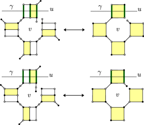
Figure 2.9: Behaviour of corner monomer insertions under urban renewal. Insertion of a monomer is modelled by the addition of edges with weight one into the dimer model: above (resp. below), the insertion of a black (resp. white) monomer at the corner $c=uv$ with a disorder operator at $u$. The green edges crossing $\gamma$ are assigned negative weights. Urban renewal is applied to the yellow quadrilaterals on the left-hand side yielding the yellow quadrilaterals on the right-hand side. Note that the colour of the monomer insertions on the left-hand and right-hand sides agree.

Lemma 2.13 (Monomer insertions in $G^{d}$ and $C_{G}$).

Let $b$ and $w$ be respectively black and white corner vertices of $G^{d}$, and let $\tilde{b}$ and $\tilde{w}$ be the corresponding black and white vertices of $C_{G}$. Then

$$Z_{G^{d}}^{\gamma}(b,w)=Z_{C_{G}}^{\gamma}(\tilde{b},\tilde{w}).$$

Proof.

We use urban renewal as in Fig. 2.9 to transform $G^{d}$ with monomer insertions to $C_{G}$ with monomer insertions. Note that here we use urban renewal with some of the long edges having negative weight. However, this is not a problem since the opposite edges in a quadrilateral being transformed by urban renewal always have the same sign, which results in a non-zero multiplicative constant for the partition functions. The resulting weights of $C_{G}$ are negative if and only if the edge crosses $\gamma$. This implies the claim readily. ∎

We finally combine the previous results to obtain the following identity. We note that it can also be derived using the approach of [Dub] after taking into account the symmetry of the underlying six-vertex model (that we do not discuss here and that is also not discussed in [Dub]).

Corollary 2.14.

In the setting of Lemma 2.12, we have

$$\langle\chi_{c_{i}}\chi_{c_{j}}\rangle=2\frac{Z^{\gamma}_{C_{G}}(w_{i},b_{j})}{Z_{C_{G}}}=2\frac{Z^{\gamma}_{C_{G}}(w_{j},b_{i})}{Z_{C_{G}}}.$$

Proof.

This follows from Lemmata 2.13 and 2.12, as well as Corollary 2.11. ∎

The final item of this section is the proof of Lemma 2.4 which explicitly computes the canonical reference 1-form (2.6) on $C_{G}$ in terms of the underlying Ising measures.

Proof of Lemma 2.4.

By the corollary above, for a street $\{w,b\}$ of $C_{G}$ corresponding to an edge $e=\{v,v^{\prime}\}$ of $G$, we have

$$\mathbf{P}^{\emptyset}_{C_{G}}(\{w,b\}\in M)=\frac{2x}{1+x^{2}}\frac{Z^{\gamma}_{C_{G}}(w,b)}{Z_{C_{G}}}=\frac{x}{1+x^{2}}\langle\chi_{c}\chi_{c^{\prime}}\rangle,$$ (2.8)

where $x=x_{e}=\tanh\beta J_{e}$ is the high-temperature Ising weight, $\tfrac{2x}{1+x^{2}}$ is the weight of the edge $\{w,b\}$ in the dimer model on $C_{G}$ as in Fig. 2.1, and where $c$ and $c^{\prime}$ are the two corners of $G$ corresponding to the two roads of $C_{G}$ that are incident on $w$ and $b$ respectively. Indeed, the first identity is a consequence of the fact that in this case the path $\gamma$ can be chosen empty and therefore the numerator $Z^{\gamma}_{C_{G}}(w,b)$ is actually the unsigned partition function of dimer covers of the graph where $w$ and $b$ are removed.

We now compute $\langle\chi_{c}\chi_{c^{\prime}}\rangle$ in terms of the Ising two-point function $\mu_{G}[\sigma_{v}\sigma_{v^{\prime}}]$. To this end, recall that $\mathcal{E}^{\emptyset}$ is the collection of sets of edges $\eta\subseteq E$ such that each vertex in the graph $(V,\eta)$ has even degree, and $\mathcal{E}^{\{v,v^{\prime}\}}$ is the collection of sets of edges such that each vertex has even degree except for $v$ and $v^{\prime}$ that have odd degree. Let

$$Z_{+}:=\mathop{\sum_{\eta\in\mathcal{E}^{\emptyset}}}_{e\in\eta}\prod_{e^{\prime}\in\eta}x_{e^{\prime}},\qquad\text{and}\qquad Z_{-}:=\mathop{\sum_{\eta\in\mathcal{E}^{\emptyset}}}_{e\notin\eta}\prod_{e^{\prime}\in\eta}x_{e^{\prime}},$$

and $Z=Z^{\emptyset}_{\text{hT}}$. By definition (2.7) of Kadanoff–Ceva fermions with $\gamma$ empty, the high-temperature expansion of spin correlations, and the fact that $\eta\mapsto\eta\triangle\{e\}$ is a bijection between $\mathcal{E}^{\emptyset}$ and $\mathcal{E}^{\{v,v^{\prime}\}}$, (2.8) gives

$$\mathbf{P}^{\emptyset}_{C_{G}}(\{w,b\}\in M)=\frac{x}{1+x^{2}}\frac{1}{Z}(x^{-1}Z_{+}+xZ_{-})=\frac{x}{1+x^{2}}\mu_{G}[\sigma_{v}\sigma_{v^{\prime}}].$$ (2.9)

The same argument applied to the other street $\{w^{\prime},b^{\prime}\}$ corresponding to the same edge $e$ yields $\mathbf{P}^{\emptyset}_{C_{G}}(\{w,b\}\in M)=\mathbf{P}^{\emptyset}_{C_{G}}(\{w^{\prime},b^{\prime}\}\in M)$ as the last displayed expression depends only on $e$. Moreover by the Kramers–Wannier duality and the same computation for the dual Ising model on the dual graph $G^{*}$, we have

$$\mathbf{P}^{\emptyset}_{C_{G}}(\{w,b^{\prime}\}\in M)=\mathbf{P}^{\emptyset}_{C_{G}}(\{w^{\prime},b\}\in M)=\frac{x^{*}}{1+(x^{*})^{2}}\mu_{G^{*}}[\sigma_{u}\sigma_{u^{\prime}}]=\ \frac{1-x^{2}}{2(1+x^{2})}\mu_{G^{*}}[\sigma_{u}\sigma_{u^{\prime}}],$$ (2.10)

where $x^{*}:=(1-x)/(1+x)$ is the dual weight, and where $\{u,u^{\prime}\}$ is the dual edge of $\{v,v^{\prime}\}$. This yields the second bullet of the lemma.

To prove the first bullet of the lemma, we need to relate the dual energy correlators $\mu_{G}[\sigma_{v}\sigma_{v^{\prime}}]$ and $\mu_{G^{*}}[\sigma_{u}\sigma_{u^{\prime}}]$ with each other. Interpreting the graphs in $\mathcal{E}^{\emptyset}$ as interfaces between spins of different value on the vertices of $G^{*}$, and using the low-temperature expansion we get

$$\mu_{G^{*}}[\sigma_{u}\sigma_{u^{\prime}}]=\frac{Z_{-}-Z_{+}}{Z}.$$

This together with the second equality of (2.9), and the fact that $Z_{+}+Z_{-}=Z$, yields

$$2x\mu_{G}[\sigma_{v}\sigma_{v^{\prime}}]+(1-x^{2})\mu_{G^{*}}[\sigma_{u}\sigma_{u^{\prime}}]=1+x^{2}.$$

Therefore adding (2.9) and (2.10) gives

$$\mathbf{P}^{\emptyset}_{C_{G}}(\{w,b\}\in M)+\mathbf{P}^{\emptyset}_{C_{G}}(\{w,b^{\prime}\}\in M)=1/2.$$

This means that the probability of seeing the road containing $w$ in the dimer configuration is $1/2$. By symmetry this is true for all roads of $C_{G}$. This finishes the proof. ∎

2.4 Kasteleyn theory and complex-valued fermionic observables

In this section, we introduce a Kasteleyn orientation which will be directly related to complex-valued observables introduced by Chelkak and Smirnov [CheSmi12].

2.4.1 A choice of Kasteleyn’s orientation

A Kasteleyn weighting of a planar bipartite graph is an assignment of complex phases $\varsigma_{e}\in\mathbb{C}$ with $|\varsigma_{e}|=1$ to the edges of the graph satisfying the alternating product condition meaning that for each cycle $e_{1},e_{2},\ldots,e_{2k}$ in the graph, we have

$$\prod_{i=1}^{k}\varsigma_{e_{2i-1}}\varsigma^{-1}_{e_{2i}}=(-1)^{k+1}.$$ (2.11)

Note that it is enough to check the condition around every bounded face of the graph.

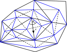
Figure 2.10: A piece of the primal graph $G$ and its dual $G^{*}$ (black solid and dashed edges respectively) and the corresponding diamond graph (blue edges) used to define the Kasteleyn weighting. Each street $e$ of $C_{G}$ can be identified with a directed edge of $G$ or $G^{*}$. Then, the angle $\theta_{e}$ is the angle in the diamond graph at the origin of this directed edge as depicted in the figure. By definition, these angles sum up to $2\pi$ around every vertex and face of $G$, and around every face of the diamond graph. This guarantees that the associated weighting satisfies the Kasteleyn condition.

To define an explicit Kasteleyn weighting for $C_{G}$, consider the diamond graph of $G$, i.e., the graph whose vertices are the vertices and faces of $G$, and whose edges are the corners of $G$ (see Fig. 2.10). Recall that the edges of $C_{G}$ that correspond to the corners of $G$ are called roads and the remaining edges (forming the quadrangles) are called streets. To each street there is assigned an angle $\theta_{e}$ between the two neighbouring corners in the diamond graph. We now define

• $\varsigma_{e}=-1$ if $e$ is a road,

• $\varsigma_{e}=\exp(\frac{\mathrm{i}}{2}\theta_{e})$ if $e$ is a street that crosses a primal edge of $G$,

• $\varsigma_{e}=\exp(-\frac{\mathrm{i}}{2}\theta_{e})$ if $e$ is a street that crosses a dual edge of $G^{*}$.

That $\varsigma$ is a Kasteleyn orientation of $C_{G}$ follows from the fact that the angles sum up to $2\pi$ around every vertex and face of $G$, and around every face of the diamond graph. Note that if $G$ is a finite subgraph of an embedded infinite graph $\Gamma$, then one can as well use the angles from the diamond graph of $\Gamma$ since, as already mentioned, one needs to check condition (2.11) only on the bounded faces of $C_{G}$. In particular, for subgraphs of the square lattice with the standard embedding, we will take $\theta_{e}=\pi/2$ for all edges $e$.

Fix a bipartite coloring of $C_{G}$, and let $K=K_{C_{G}}$ be a Kasteleyn matrix for a dimer model on the bipartite graph $C_{G}$ with the weighting as above, i.e., the matrix whose rows are indexed by the black vertices and the columns by the white vertices, and whose entries are

$$K(b,w):=\varsigma_{bw}x_{bw}$$

if $bw$ is an edge of $C_{G}$ and $K(b,w)=0$ otherwise, where $b$ and $w$ are respectively black and white vertices, and $x$ is the edge weight for $C_{G}$ as in Fig. 2.1.

We assume that the set of corners of $G$ comes with a prescribed order $c_{1},\ldots,c_{m}$, and we order the rows and columns of $K$ according to this order (for each white and black vertex of $C_{G}$, there is exactly one corner of $G$ that the vertex corresponds to). We denote by $b_{i}$ and $w_{i}$ the black and white vertex of $C_{G}$ corresponding to $c_{i}$.

The following lemma is a known observation.

Lemma 2.15.

We have that

$$K^{-1}(w_{i},b_{j})=\mathrm{i}\kappa_{\gamma}\frac{Z^{\gamma}_{C_{G}}(w_{i},b_{j})}{Z_{C_{G}}},$$ (2.12)

where $\gamma$ is a dual path connecting a face $u_{i}$ adjacent to $b_{i}$ with a face $u_{j}$ adjacent to $w_{j}$, $\kappa_{\gamma}$ is a global complex phase depending only on $\gamma$ given by

$$\kappa_{\gamma}=(-1)^{i+j+1+N}\textnormal{sgn}(\pi)\mathrm{i}\prod_{k=1}^{m-1}\tilde{\varsigma}_{\tilde{b}_{k}\tilde{w}_{\pi(k)}},$$ (2.13)

and $Z^{\gamma}_{C_{G}}(b_{i},w_{j})$ is the partition function of dimers on $C_{G}$ with $b_{i}$ and $w_{j}$ removed, and with negative weights assigned to the edges crossing $\gamma$.

The factor $\mathrm{i}$ is due to an arbitrary choice of $\kappa_{\gamma}$ which is made for later convenience. We will now justify (2.12) and explicitly identify the complex phase $\kappa_{\gamma}$ in this expression.

Proof.

To compute the inverse matrix, we use the cofactor representation as a ratio of determinants:

$$K^{-1}(w_{i},b_{j})=(-1)^{i+j}\frac{\det K^{b_{j},w_{i}}}{\det K},$$

where $K^{w_{i},b_{j}}=:\tilde{K}$ is the matrix $K$ with the $j$-th row and $i$-th column removed.

By definition of the determinant, we have

$$\det K=\sum_{\pi\in S_{m}}\textnormal{sgn}(\pi)\prod_{k=1}^{m}\varsigma_{b_{k}w_{\pi(k)}}x_{b_{k}w_{\pi(k)}}.$$

In this sum, only terms where $\pi$ corresponds to a perfect matching on $C_{G}$ are nonzero. Moreover, by a classical theorem of Kasteleyn [Kasteleyn], the complex phase $\textnormal{sgn}(\pi)\prod_{i=1}^{m}\varsigma_{b_{i}w_{\pi(i)}}$ is constant for such $\pi$. In particular, we can take $\pi$ to be the identity. Since $\varsigma_{b_{i}w_{i}}=-1$, we get that

$$\det K=(-1)^{N}Z_{C_{G}},$$

where $N$ is the number of corner edges in $C_{G}$.

We now want to interpret $\tilde{K}$ as a Kasteleyn matrix for the graph $\tilde{C}_{G}$ obtained from $C_{G}$ by removing the vertices $w_{i}$ and $b_{j}$. To this end, if $w_{i}$ and $b_{j}$ are not incident on the same face $u_{i}=u_{j}$, we need to introduce a sign change to the Kasteleyn weighting along a dual path $\gamma$ which connects $u_{i}$ to $u_{j}$. We do it as follows. Define modified weights $\tilde{\varsigma}$ and $\tilde{x}$ by $\tilde{\varsigma}_{e}=-\varsigma_{e}$ (resp. $\tilde{x}_{e}=-x_{e}$), if $e$ is crossed by $\gamma$, and $\tilde{\varsigma}_{e}=\varsigma_{e}$ (resp. $\tilde{x}_{e}=x_{e}$) otherwise. Then $\varsigma_{e}x_{e}=\tilde{\varsigma}_{e}\tilde{x}_{e}$, and hence $\tilde{K}(b,w)=\tilde{\varsigma}_{bw}\tilde{x}_{bw}$ if $bw$ is an edge of $\tilde{C}_{G}$, and $\tilde{K}(b,w)=0$ otherwise. We leave it to the reader to verify that $\tilde{\varsigma}$ is indeed a Kasteleyn weighting for $\tilde{C}_{G}$.

We can therefore again apply Kasteleyn’s theorem to obtain

$$\det\tilde{K}=\sum_{\pi\in S_{m-1}}\textnormal{sgn}(\pi)\prod_{k=1}^{m-1}\tilde{\varsigma}_{\tilde{b}_{k}\tilde{w}_{\pi(k)}}\tilde{x}_{b_{k}w_{\pi(k)}}=\tilde{\kappa}_{\gamma}{Z^{\gamma}_{C_{G}}(w_{i},b_{j})},$$

where $\tilde{b}_{1},\ldots,\tilde{b}_{m-1}$ (resp. $\tilde{w}_{1},\ldots,\tilde{w}_{m-1}$) is an order preserving renumbering of the black (resp. white) vertices where $b_{j}$ (resp. $w_{i}$) is removed. Again,

$$\tilde{\kappa}_{\gamma}=\textnormal{sgn}(\pi)\prod_{k=1}^{m-1}\tilde{\varsigma}_{\tilde{b}_{k}\tilde{w}_{\pi(k)}}$$

is a constant complex factor independent of the permutation $\pi$ defining a perfect matching of $\tilde{C}_{G}$. This justifies (2.12). ∎

We now proceed to giving $\kappa_{\gamma}$ a concrete representation in terms of the winding angle of $\gamma$. To this end, we first need to introduce some complex factors. We follow [CCK] and for each directed edge or corner $e$, we fix a square root of the corresponding direction in the complex plane and denote by $\eta_{e}$ its complex conjugate. Recall that we always assume that a corner $c$ is oriented towards its vertex $v(c)$, and we write $-c$ whenever we consider the opposite orientation. For two directed edges or corners $e,g$ that do not point in opposite directions, we define $\angle(e,g)$ to be the turning angle from $e$ to $g$, i.e., the number in $(-\pi,\pi)$ satisfying

$$e^{-\mathrm{i}\angle(e,g)}=(\overline{\eta_{e}}\eta_{g})^{2}.$$

Lemma 2.16.

Let $c_{i}$, $c_{j}$, and $\gamma$ be as above. Define $\tilde{\gamma}$ to be the extended path starting at $-c_{j}$, following $\gamma$, and ending at $c_{i}$. Then,

$$\kappa_{\gamma}=\exp(\tfrac{\mathrm{i}}{2}\textnormal{wind}(\tilde{\gamma})),$$

where $\textnormal{wind}(\tilde{\gamma})$ is the total winding angle of the path $\tilde{\gamma}$, i.e., the sum of all turning angles along the path.

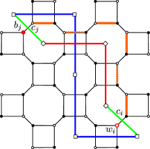
Figure 2.11: An illustration of the proof of Lemma 2.16 in the case where $G$ is a piece of the square lattice. The green lines represent corners $c_{i}$ and $c_{j}$, the red lines represent the primal path $\rho$ from $v(c_{i})$ to $v(c_{j})$, and the blue lines show the dual path $\gamma$ from $u(c_{j})$ to $u(c_{i})$. The red vertices $w_{i}$ and $b_{j}$ are removed in the graph $C_{\tilde{G}}$. The matching $M_{\rho}$ corresponding to $\rho$ contains the orange streets and all remaining roads. The dashed (resp. solid) orange edges carry a phase $\exp({\tfrac{\mathrm{i}\pi}{4}})$ (resp. $\exp(-{\tfrac{\mathrm{i}\pi}{4}})$) in the original Kasteleyn weighting $\varsigma$ of $C_{G}$. The orange edge crossed by $\gamma$ gets an additional $-1$ sign in the Kasteleyn weighting $\tilde{\varsigma}$ of $\tilde{C}_{G}$.

Proof.

Let $\rho$ be a simple primal path starting at $v(c_{i})$ and ending at $v(c_{j})$, and let $\tilde{\rho}$ be the extended path that starts at $c_{i}$, then follows $\rho$, and ends at $-c_{j}$. We will define a perfect matching $M_{\rho}$ of $\tilde{C}_{G}$ that corresponds to $\rho$ in a natural way (see Fig. 2.11). Note that there is a unique sequence of streets $S_{\rho}$ such that the first edge contains $b_{i}$ and the last edge contains $w_{j}$, and where all the edges are directly to the right of the oriented path $\tilde{\rho}$ (the orange edges in Fig. 2.11). We define $M_{\rho}$ to contain $S_{\rho}$ and all the remaining roads denoted by $R_{\rho}$.

Moreover, let $\ell$ be the loop (closed path) which is the concatenation of $\tilde{\rho}$ and $\tilde{\gamma}$. We claim that

$$\prod_{bw\in S_{\rho}}\tilde{\varsigma}_{bw}=(-1)^{t(\ell)}\prod_{bw\in S_{\rho}}\varsigma_{bw}=(-1)^{t(\ell)+1}\mathrm{i}\exp(-\tfrac{\mathrm{i}}{2}\textnormal{wind}(\tilde{\rho})),$$ (2.14)

where $t(\ell)$ is the number of self-crossings of $\ell$. Indeed, the first identity follows since the self-crossings of $\ell$ only come from a crossing between $\gamma$ and $\rho$, and each such edge gets an additional $-1$ factor in the Kasteleyn weighting $\tilde{\sigma}$. We now argue for the second inequality by inspecting the contribution of the phases $\varsigma$ at each turn of $\tilde{\rho}$.

Figure 2.12: An illustration of the proof of (2.14). The path $\rho$ goes from $c_{i}$ to $-c_{j}$, and is composed of the two red edges. The orange edges represent $S_{\rho}$.

To this end we consider all the corners adjacent to $\rho$. We denote by $\alpha_{k}$ (resp. $\alpha^{*}_{k}$), $k=1,2,\ldots,$ the unsigned angles between two consecutive corners that share a vertex (resp. a face) of $G$, and by $\beta_{k}$ we denote the angles between the edges of $\rho$ and the corners (see Fig. 2.12). Note that there is exactly $|\rho|$ angles of type $\alpha^{*}$, and $2|\rho|$ angles of type $\beta$ (there can be more angles of type $\alpha$). Moreover, $\alpha^{*}_{k}=\pi-\beta_{2k-1}-\beta_{2k}$ for each $k\in\{1,\ldots,|\rho|\}$. Finally, the sum of all angles of type $\alpha$ and $\beta$ around a vertex of $G$ is by definition equal to $\pi$ plus the turning angle of $\rho$ at that vertex. Writing $A$ (resp. $B$) for the sum of all angles of type $\alpha$ (resp. $\beta$), and using the definition of $\varsigma$, we find

$$\prod_{bw\in S_{\rho}}\varsigma_{bw}=\prod_{k}e^{-\tfrac{\mathrm{i}\alpha_{k}}{2}}\prod_{k}e^{\tfrac{\mathrm{i}\alpha^{*}_{k}}{2}}=e^{{-\tfrac{\mathrm{i}}{2}(A+B-|\rho|\pi)}}=e^{{-\tfrac{\mathrm{i}}{2}(\textnormal{wind}(\tilde{\rho})+\pi)}}=-\mathrm{i}\exp({-\tfrac{\mathrm{i}}{2}\textnormal{wind}(\tilde{\rho})}),$$

which justifies (2.14).

On the other hand, a classical fact due to Whitney [Whi] (see also [CCK, Lemma 2.2]) says that

$$\exp(\tfrac{\mathrm{i}}{2}\textnormal{wind}(\ell))=(-1)^{t(\ell)+1}.$$ (2.15)

Factorizing the left-hand side into the contributions coming from $\tilde{\rho}$ and $\tilde{\gamma}$, we get

$$\exp(\tfrac{\mathrm{i}}{2}\textnormal{wind}(\ell))=\kappa_{\gamma}\exp(\tfrac{\mathrm{i}}{2}\textnormal{wind}(\tilde{\rho})).$$

Combining with (2.14) we arrive at

$$\prod_{bw\in M_{\rho}}\tilde{\varsigma}_{bw}=\prod_{bw\in S_{\rho}}\tilde{\varsigma}_{bw}\prod_{bw\in R_{\rho}}\tilde{\varsigma}_{bw}=(-1)^{|R_{\rho}|}\mathrm{i}\kappa_{\gamma},$$

where the second equality holds true since roads have complex phase $\varsigma=-1$. On the other hand, by (2.13) we have

$$\kappa_{\gamma}=(-1)^{i+j+1+N}\textnormal{sgn}(\pi)\mathrm{i}\prod_{k=1}^{m-1}\tilde{\varsigma}_{b_{k}w_{\pi(k)}}=(-1)^{i+j+1+N}\textnormal{sgn}(\pi)\mathrm{i}\prod_{bw\in M_{\rho}}\tilde{\varsigma}_{bw},$$

where $\pi\in S_{k-1}$ is the permutation defining the matching $M_{\rho}$, and $N$ is the number of all corner edges in $C_{G}$. Therefore to finish the proof, it is enough to show that

$$\textnormal{sgn}(\pi)=(-1)^{i+j+N+|R_{\rho}|}.$$ (2.16)

To this end, first note that $M_{\rho}$ naturally defines a bijection $\tilde{\pi}$ of the set of corners of $G$ with the two corners $c_{i}$ and $c_{j}$ identified as one corner, called from now on $\tilde{c}$, where $\tilde{\pi}(c)=c^{\prime}$ if the black vertex corresponding to $c$ is connected by an edge in $M_{\rho}$ to the white vertex corresponding to $c^{\prime}$. This bijection can be thought of as a permutation of $\{1,\ldots,k-1\}$ where the index corresponding to $\tilde{c}$ is $m-1$, and where the first $m-2$ indices respect the original order on the remaining corners of $C_{G}$. Clearly $\tilde{\pi}$ has only one nontrivial cycle whose length is $|S_{\rho}|+1$, and hence $\textnormal{sgn}(\tilde{\pi})=(-1)^{|S_{\rho}|}$. Without loss of generality, let $j>i$ and for an index $l\in\{1,\ldots,k-1\}$, let $p_{l}\in S_{k-1}$ be the permutation such that $p_{l}(l)=k-1$ and that does not change the order of the remaining indices. Note that $\textnormal{sgn}(p_{l})=(-1)^{k-1-l}$ as $p_{l}$ is a composition of $k-1-l$ transpositions. One can check that $\pi=p_{i}^{-1}\tilde{\pi}p_{j-1}$, and as a result $\textnormal{sgn}(\pi)=(-1)^{i+j-1+|S_{\rho}|}$. To show (2.16) and finish the proof, we count the roads whose both endpoints are covered by a street in $S_{\rho}$, to get that $N=|S_{\rho}|+1+|R_{\rho}|$. ∎

All in all, from (2.12) together with Corollary 2.14 we obtain the following statement.

Corollary 2.17.

We have

$$K^{-1}(w_{i},b_{j})=\tfrac{1}{2}\mathrm{i}\kappa_{\gamma}\langle\chi_{c_{i}}\chi_{c_{j}}\rangle,$$ (2.17)

where the complex phase $\kappa_{\gamma}$ is as in Lemma 2.16.

2.4.2 Complex-valued fermionic observables

In this section we rewrite $\langle\chi_{c_{i}}\chi_{c_{j}}\rangle$, and hence the right-hand side of (2.17), in terms of complex-valued fermionic observables of Chelkak–Smirnov [CheSmi12], and Hongler–Smirnov [HonSmi]. This correspondence is well-known (and can be e.g. found in [CCK]) but we choose to present the details for completeness of exposition. In the next section, we will use it together with the available scaling limit results to derive the scaling limit of $K^{-1}$ for the critical model on $C_{D^{\delta}}$.

We first define the complex version of the Kadanoff–Ceva observable for two corners $c_{i}$ and $c_{j}$ by

$$f(c_{i},c_{j}):=\frac{1}{Z^{\emptyset}_{\text{hT}}}\sum_{\eta\in\mathcal{E}^{v(c_{i}),v(c_{j})}}\exp(-\tfrac{\mathrm{i}}{2}\textnormal{wind}(\rho_{\eta}))\prod_{e\in\eta}x_{e},$$ (2.18)

where $\textnormal{wind}(\rho_{\eta})$ is again the total winding angle of the path $\rho_{\eta}$, i.e. the sum of all turning angles along the path, and where $\rho_{\eta}$ is a simple path contained in $\eta\cup\{c_{i},c_{j}\}$ that starts at $c_{i}$ and ends at $-c_{j}$, and is defined as follows: for each vertex $v$ of degree larger than two in $\eta$, one connects the edges around $v$ into pairs in a non-crossing way, thus giving rise to a collection of non-crossing cycles $\mathcal{C}_{\eta}$ and a path from $c_{i}$ to $-c_{j}$ that we call $\rho_{\eta}$.

It is a standard fact that the definition of $f(c_{i},c_{j})$ does not depend on the way the connections at each vertex of $\eta$ are chosen (as long as they are noncrossing). Moreover, for all $\eta\in\mathcal{E}^{v(c_{i}),v(c_{j})}$, we have

$$-\overline{\kappa}_{\gamma}\exp(-\tfrac{\mathrm{i}}{2}\textnormal{wind}(\rho_{\eta}))=\textnormal{sgn}_{\gamma}(\eta),$$ (2.19)

where as before, $\gamma$ is a fixed dual path connecting $u(c_{i})$ and $u(c_{j})$, and $\kappa_{\gamma}=\exp(\tfrac{\mathrm{i}}{2}\textnormal{wind}(\tilde{\gamma}))$, with $\tilde{\gamma}$ being the path starting at $-c_{j}$, then following $\gamma$, and ending at $c_{i}$. To justify this identity, we consider the loop $\ell$ which is the concatenation of $\rho_{\eta}$ and the path $\tilde{\gamma}$, and write

$$\exp(-\tfrac{\mathrm{i}}{2}\textnormal{wind}(\ell))=\overline{\kappa}_{\gamma}\exp(-\tfrac{\mathrm{i}}{2}\textnormal{wind}(\rho_{\eta})).$$

We then again use Whitney’s identity (2.15) and the fact that the collection of cycles $\mathcal{C}_{\eta}$ must, by construction, cross $\gamma$ an even number of times (since $\mathcal{C}_{\eta}$ does not cross $\rho_{\eta}$, and $\mathcal{C}_{\eta}$ crosses $\ell$ an even number of times for topological reasons). This justifies (2.19) and implies that

$$\langle\chi_{c_{i}}\chi_{c_{j}}\rangle=-\overline{\kappa}_{\gamma}f(c_{i},c_{j}),$$

which together with Corollary 2.17 gives the following proposition.

Proposition 2.18.

We have

$$K^{-1}(w_{i},b_{j})=-\tfrac{\mathrm{i}}{2}f(c_{i},c_{j}).$$ (2.20)

To make the connection with the scaling limit results of [HonSmi], we still need to introduce an observable that is indexed by two directed edges of $G$ instead of two corners. To this end, for each edge $e$ of $G$, let $z_{e}$ be its midpoint. Also, for a directed edge $e=(v_{1},v_{2})$, let $h(e)$ be the half-edge $\{z_{e},v_{2}\}$, let $-e=(v_{2},v_{1})$ be its reversal, and let $\bar{e}=\{v_{1},v_{2}\}$ be its undirected version. Moreover, for two directed edges $e=(v_{1},v_{2})$ and $g=(\tilde{v}_{1},\tilde{v}_{2})$, let $\mathcal{E}^{e,g}$ be the collections of edges $\tilde{\eta}\in\mathcal{E}^{v_{2},\tilde{v}_{1}}$ that do not contain $\bar{e}$ and $\bar{g}$. We define

$$f(e,g):=\frac{1}{Z^{\emptyset}_{\text{hT}}}\sum_{\tilde{\eta}\in\mathcal{E}^{e,g}}\exp(-\tfrac{\mathrm{i}}{2}\textnormal{wind}(\rho_{\tilde{\eta}}))\prod_{e\in\tilde{\eta}}x_{e},$$

where $\rho_{\tilde{\eta}}$ is a simple path in $\tilde{\eta}\cup\{h(e),h(-g)\}$ that starts at $z_{e}$ and ends at $z_{g}$, and is analogous to $\rho_{\eta}$ from (2.18). Note that the winding of $\rho_{\tilde{\eta}}$ is constant (independent of $\tilde{\eta}$) modulo $2\pi$ and equal to $\angle(e,g)$, and therefore

$$f(e,g)\in\overline{\eta}_{e}{\eta}_{g}\mathbb{R}.$$ (2.21)

3 Proof of Theorem 1.3

Let $D$ be a bounded simply connected domain, and let $D^{\delta}$ be an approximation of $D$ by $\delta\mathbb{Z}^{2}$. We consider the critical double random current model with free boundary conditions on $D^{\delta}$, and the corresponding dimer model on Dubédat’s square-octagon graph $C_{D^{\delta}}$. We call $U^{\delta}$ and $V^{\delta}$ the set of faces of $C_{D^{\delta}}$ that correspond to the faces and vertices of $D^{\delta}$ respectively. In this section we show that the moments of the associated height function $h^{\delta}$ converge to the moments of $\frac{1}{\sqrt{\pi}}$ times the Dirichlet GFF.

3.1 Scaling limit of inverse Kasteleyn matrix

We start by establishing the scaling limit of the inverse Kasteleyn matrix on $C_{D^{\delta}}$. This is crucial for the computation of the moments of the height function that is done in the next section.

Our method is to use Proposition 2.18 obtained in the previous section, as well as the existing scaling limit results for discrete s-holomorphic observables in the Ising model [CHI, HonSmi]. It is important to note that for the purpose of proving the main conjecture of Wilson, we need to work with continuum domains $D$ with an arbitrary (possibly fractal) boundary. Therefore, we state a generalized version of the scaling limit results of Hongler and Smirnov [HonSmi] for the critical fermionic observable with two points in the bulk of the domain. Their result, as stated, is valid only for domains whose boundary is a rectifiable curve (see also [hongler]). Even though the stronger result that we need is most likely known to the experts, for the sake of completeness, we will outline its proof, which is a direct consequence of the robust framework of Chelkak, Hongler and Izyurov [CHI] that was used to establish scaling limits for critical spin correlations.

From now on, we assume that the observables are critical, i.e., the weight $x_{e}$ is constant and equal to $x_{c}=\sqrt{2}-1$ so that $\prod_{e\in\eta}x_{e}=x_{c}^{|\eta|}$. Also, we define

$$f(e,z_{g}):=x_{c}(f(e,g)+f(e,-g)),$$ (3.1)

which is the observable of Hongler and Smirnov [HonSmi] (when $e$ is a horizontal edge pointing to the right) that is indexed by a directed edge $e$ and a midpoint of an edge $z_{g}$. The next lemma relates this observable to the corner observable in a linear fashion. This type of identities is well known (see e.g. [CCK]) and is closely related to the notion of s-holomorphicity introduced by Smirnov [smirnov] for the square lattice, and generalized by Chelkak and Smirnov [CheSmi12], and Chelkak [Che17, Che20]. We omit the proof.

Lemma 3.1.

Let $c_{i}$ and $c_{j}$ be two corners that do not share a vertex, and let $e$ and $g$ be directed edges incident to $v(c_{i})$ and $v(c_{j})$ respectively. Then

$$f(c_{i},c_{j})=\frac{1}{\sqrt{2}}\sum_{e^{\prime}\in\{e,-{e}\}}\big{(}1+(\overline{\eta_{c_{i}}}\eta_{e^{\prime}})^{2}\big{)}\big{(}f(e^{\prime},z_{g})-(\overline{\eta_{e^{\prime}}}{\eta_{c_{j}}})^{2}\overline{f(e^{\prime},z_{g})}\big{)}.$$

We also need to introduce the continuum counterparts of the discrete holomorphic observables. To this end, let $D\subsetneq\mathbb{C}$ be a simply connected domain different from $\mathbb{C}$, and let $\psi_{w}=\psi^{D}_{w}$ be the unique conformal map from $D$ to the unit disk with $\psi_{w}(w)=0$ and $\psi^{\prime}_{w}(w)>0$. For $w,z\in D$, we define

$$f_{-}^{D}(w,z):=\frac{1}{2\pi}\sqrt{\psi_{w}^{\prime}(w)\psi_{w}^{\prime}(z)}\quad\text{and}\quad f_{+}^{D}(w,z):=\frac{1}{2\pi}\sqrt{\psi_{w}^{\prime}(w)\psi_{w}^{\prime}(z)}\frac{1}{\psi_{w}(z)}.$$

Lemma 3.2 (Conformal covariance of $f^{D}_{\pm}$).

Let $\varphi:D\to D^{\prime}$ be a conformal map. Then

$$f_{-}^{D}(w,z) ={\overline{\varphi^{\prime}(w)}}^{\tfrac{1}{2}}{\varphi^{\prime}(z)}^{\tfrac{1}{2}}f_{-}^{D^{\prime}}(\varphi(w),\varphi(z)),$$

$$f_{+}^{D}(w,z) ={{\varphi^{\prime}(w)}}^{\tfrac{1}{2}}{\varphi^{\prime}(z)}^{\tfrac{1}{2}}f_{+}^{D^{\prime}}(\varphi(w),\varphi(z)).$$

Moreover, for the upper half-plane $\mathbb{H}$, we have

$$f_{-}^{\mathbb{H}}(w,z)=\frac{\mathrm{i}}{2\pi(z-\overline{w})}\quad\text{and}\quad f_{+}^{\mathbb{H}}(w,z)=\frac{1}{2\pi(z-w)}.$$

Proof.

To prove the first part, note that $\psi^{D^{\prime}}_{\varphi(w)}(z)=\psi_{w}^{D}(\varphi^{-1}(z))\frac{\varphi^{\prime}(w)}{|\varphi^{\prime}(w)|}$. Indeed, the right-hand side is a conformal map with a positive derivative $(\psi_{w}^{D})^{\prime}(w)/|\varphi^{\prime}(w)|$ and vanishing at $\varphi(w)$. Hence we have

$$f_{-}^{D^{\prime}}(\varphi(w),\varphi(z)) =[(\psi^{D^{\prime}}_{\varphi(w)})^{\prime}(\varphi(w))(\psi^{D^{\prime}}_{\varphi(w)})^{\prime}(\varphi(z))]^{\tfrac{1}{2}}$$

$$=[(\psi^{D}_{w})^{\prime}(w)(\psi^{D}_{w})^{\prime}(z)]^{\frac{1}{2}}[{\varphi^{\prime}(w)\varphi^{\prime}(z)]^{-\tfrac{1}{2}}}\frac{\varphi^{\prime}(w)}{|\varphi^{\prime}(w)|}$$

$$=f_{-}^{D}(w,z){\overline{\varphi^{\prime}(w)}^{-\tfrac{1}{2}}\varphi^{\prime}(z)^{-\tfrac{1}{2}}},$$

and similarly for $f^{D}_{+}$. The second part follows from the fact that $\psi^{\mathbb{H}}_{w}(z)=i\frac{z-w}{z-\overline{w}}$ and the definition of $f_{\pm}^{\mathbb{H}}$. ∎

We now proceed to the generalization of [HonSmi, Theorem 8] mentioned at the beginning of the section. In the proof we will very closely follow the proof of [CHI, Theorem 2.16] dealing with the convergence of discrete s-holomorphic spinors.

Theorem 3.3.

Let $D\subsetneq\mathbb{C}$ be a bounded simply connected domain, and let $D^{\delta}$ approximate $D$ as $\delta\to 0.$ Fix $w,z\in D$, and let $e=e^{\delta}$ and $g=g^{\delta}$ be edges of $D^{\delta}$ whose midpoints converge to $w$ and $z$ respectively as $\delta\to 0$. Then

$$f^{{\delta}}(e,z_{g})=\delta\big{(}f_{-}^{D}(w,z)+{\overline{\eta}_{e}^{2}}f_{+}^{D}(w,z)+o(1)\big{)}\qquad\text{as }\delta\to 0,$$

where $f^{\delta}$ is the observable from (3.1) defined on $D^{\delta}$. Moreover the convergence is uniform on compact subsets of $\{(w,z)\in D^{2}:w\neq z\}$.

Before giving a sketch of the proof of this theorem, we state a corollary that will be convenient for us when computing moments of the height function in the next section.

Corollary 3.4.

Consider the setting from the lemma above and let $c_{i}=c_{i}^{\delta}$ and $c_{j}=c_{j}^{\delta}$ be two corners of $D^{\delta}$ whose vertices converge to $w$ and $z$ respectively. Then

$$K^{-1}(w_{i},b_{j}) =-\frac{1}{\sqrt{2}}{\delta\mathrm{i}}\big{(}f^{D}_{-}(w,z)-\overline{\eta}_{c_{i}}^{2}\eta_{c_{j}}^{2}\overline{f^{D}_{-}(w,z)}+\overline{\eta}^{2}_{c_{i}}f^{D}_{+}(w,z)-{\eta^{2}_{c_{j}}}\overline{f^{D}_{+}(w,z)}+o(1)\big{)},$$

where $K^{-1}$ is the inverse Kasteleyn matrix on $C_{D^{\delta}}$.

Proof.

To simplify the notation, we drop $D$ from the superscripts. We combine Lemma 3.3 and Lemma 3.1 to get that $\frac{\sqrt{2}}{\delta}f(c_{i},c_{j})$ equals to

$$\sum_{e^{\prime}\in\{e,-e\}}\big{(}1+(\overline{\eta}_{c_{i}}\eta_{e^{\prime}})^{2})(f(e^{\prime},z_{g})-(\overline{\eta}_{e^{\prime}}{\eta_{c_{j}}})^{2}\overline{f(e^{\prime},z_{g})})$$

$$=\sum_{e^{\prime}\in\{e,-e\}}\big{(}1+(\overline{\eta}_{c_{i}}\eta_{e^{\prime}})^{2})(f_{-}(w,z)+\overline{\eta}_{e^{\prime}}^{2}f_{+}(w,z)-(\overline{\eta}_{e^{\prime}}{\eta_{c_{j}}})^{2}\overline{f_{-}(w,z)}-\eta_{c_{j}}^{2}\overline{f_{+}(w,z)})+o(1)$$

$$=2\big{(}f_{-}(w,z)+\overline{\eta}_{c_{i}}^{2}f_{+}(w,z)-\overline{\eta}_{c_{i}}^{2}{\eta^{2}_{c_{j}}\overline{f_{-}(w,z)}}-{\eta_{c_{j}}^{2}\overline{f_{+}(w,z)}}\big{)}+o(1),$$

where the last equality holds due to cancellations resulting from $\eta_{e}^{2}=-\eta_{-e}^{2}$. On the other hand, by (2.20), $K^{-1}(w_{i},b_{j})=-\tfrac{\mathrm{i}}{2}f(c_{i},c_{j})$ which finishes the proof. ∎

Sketch of proof of Theorem 3.3.

Based on the scaling limit results of Hongler–Smirnov [HonSmi], we first argue that the statement holds true for a domain $D$ with a smooth boundary. Indeed, in [HonSmi] it is assumed that $\eta_{e}^{2}=1$ and hence, in that case, the result follows directly from [HonSmi, Theorem 8]. Applying this to a rotated domain together with the conformal covariance properties from Lemma 3.2 yields the statement for a general direction of $e$.

We now briefly describe how to use the robust framework of Chelkak, Hongler and Izyurov to extend this to general simply connected domains. In [CHI, Theorem 2.16], a scaling limit result was established for a discrete holomorphic spinor $F^{\delta}$ defined on an approximation $D^{\delta}$ of an arbitrary bounded simply connected domain $D$. The two observables $F^{\delta}$ and $f^{\delta}$ satisfy the same boundary conditions (of [HonSmi, Proposition 18] and [CHI, (2.7)]). Moreover, both observables are s-holomorphic away from the diagonal. The difference however is their singular behaviour near the diagonal. In [CHI], the full plane version $F_{\mathbb{C}}^{\delta}$ (the discrete analog of $1/\sqrt{z-w}$) of the observable is subtracted from $F^{\delta}$ in order to cancel out the discrete-holomorphic singularity on the diagonal. The details of the proof of [CHI, Theorem 2.16] can be carried out verbatim for $f^{\delta}$ instead of $F^{\delta}$ and its full plane version $f_{\mathbb{C}}^{\delta}$ (the discrete analog of $1/(z-w)$) introduced in [HonSmi] instead of $F_{\mathbb{C}}^{\delta}$. Indeed, the arguments in [CHI] depend only on the fact that the observables in question are s-holomorphic and satisfy the correct boundary value problem.

Since the scaling limit is conformally invariant and was uniquely identified for domains with a smooth boundary by the argument above. This finishes the proof. ∎

3.2 Moments of $h^{\delta}$

For simplicity of exposition, we only consider the height function on $C_{D^{\delta}}$ restricted to $U^{\delta}$ which has the same distribution as the nesting field of the critical double random current on $D$ with free boundary conditions. The case of mixed moments (for the joint height function on both the faces and vertices of $D^{\delta}$) follows in the same manner as the faces and vertices of $D^{\delta}$ play a symmetric role in the graph $C_{D^{\delta}}$. To this end, let $a_{1},a_{2},\ldots,a_{n}$ be distinct points in $D$, and let $h^{\delta}(a_{i})$ $(i=1,\ldots,n)$ be the height function evaluated at the face $u^{\delta}_{i}=u^{\delta}_{i}(a_{i})\in U^{\delta}$ of $D^{\delta}$, in which the point $a_{i}$ lies (we choose a face arbitrarily if $a_{i}$ lies on an edge of $D^{\delta}$).

Let $G_{D}(z,w)$ be the Dirichlet Green’s function in $D$, i.e., the Green’s function of standard Brownian motion in $D$ killed upon hitting $\partial D$. In particular for the upper-half plane $\mathbb{H}$, we have

$$G_{\mathbb{H}}(z,w)=\frac{1}{2\pi}\ln\Big{|}\frac{z-\overline{w}}{z-w}\Big{|}.$$

This section is devoted to the proof of the following theorem. Below, $\mathbf{P}^{\emptyset,\emptyset}_{D^{\delta},D^{\delta}}$ denotes the probability measure of the double random current model with free boundary conditions together with the independent labels used to define the nesting field.

Theorem 3.5.

For every even integer $n$ and any distinct points $a_{1},a_{2},\ldots,a_{n}\in D$, we have

$$\lim_{\delta\rightarrow 0}\mathbf{E}^{\emptyset,\emptyset}_{D^{\delta},D^{\delta}}\Big{[}\prod_{i=1}^{n}h^{\delta}(a_{i})\Big{]}=\sum_{\pi\text{ pairing of }\{a_{1},\dots,a_{n}\}}\prod_{\{z,w\}\in\pi}\tfrac{1}{\pi}G_{D}(z,w),$$

where a pairing is a partition into sets of size two.

Note that the field $h^{\delta}$ is symmetric, and therefore the corresponding moments for $n$ odd vanish.

In the proof of the theorem, we follow the line of computation due to Kenyon [Ken00] but with several adjustments to our setting. In particular, we start with an algebraic manipulation to take care of the behaviour of $K^{-1}$ near the boundary of $D^{\delta}$: for $a_{1}^{0},\ldots,a_{n}^{0}\in D$, write

$$\mathbf{E}^{\emptyset,\emptyset}_{D^{\delta},D^{\delta}}\Big{[}\prod_{i=1}^{n}h^{\delta}(a_{i})\Big{]} =\mathbf{E}^{\emptyset,\emptyset}_{D^{\delta},D^{\delta}}\Big{[}\prod_{i=1}^{n}(h^{\delta}(a_{i})-h^{\delta}(a_{i}^{0}))\Big{]}-\mathop{\sum_{t\in\{0,1\}^{n}}}_{t\neq(1,\ldots,1)}(-1)^{\sum_{i}(1-t_{i})}\mathbf{E}^{\emptyset,\emptyset}_{D^{\delta},D^{\delta}}\Big{[}\prod_{i=1}^{n}h^{\delta}(a_{i}^{t_{i}})\Big{]},$$ (3.2)

where $a_{i}^{1}=a_{i}$ for $i=1,\dots,n$.

The advantage of this formulation is that the first term on the right-hand side can be computed using Kasteleyn theory, and that the others are small when $a_{1}^{0},\ldots,a_{n}^{0}$ are close to the boundary. This latter fact is not obvious and is relying on discrete properties of the double random current obtained in [DumLisQia21] (note that it is basically saying that the field is uniformly small – in terms of moments – near the boundary).

We start by proving that the remaining terms are small.

Proposition 3.6.

For any $\varepsilon>0$ and $a_{1},\dots,a_{n}\in D$, one may choose $a_{1}^{0},\ldots,a_{n}^{0}\in D$ so that

$$\Big{|}\mathbf{E}^{\emptyset,\emptyset}_{D^{\delta},D^{\delta}}\Big{[}\prod_{i=1}^{n}h^{\delta}(a_{i})\Big{]}-\mathbf{E}^{\emptyset,\emptyset}_{D^{\delta},D^{\delta}}\Big{[}\prod_{i=1}^{n}(h^{\delta}(a_{i})-h^{\delta}(a_{i}^{0}))\Big{]}\Big{|}<\varepsilon$$ (3.3)

uniformly in $\delta>0$.

Remark 3.7.

This proposition, which basically claims that the second term on the right-hand side of (3.2) is approximately zero provided the $a_{i}^{0}$ are close enough to the boundary, is a restatement of the fact that boundary conditions for the limiting height function are zero. It is therefore the main place where we identify boundary conditions. Note that this proposition relies heavily on the main result in [DumLisQia21] and is as such non-trivial.

To prove this proposition, we need to introduce some auxiliary notions. We say that a cluster of the double random current is relevant for $A=\{a_{1},\ldots,a_{n}\}\subsetneq D$ if it is odd around $u_{i}^{\delta}$ for at least two different $i\in\{1,\ldots,n\}$ (it is possible that $u^{\delta}_{i}=u^{\delta}_{j}$ even though $a_{i}\neq a_{j}$). We denote by $\mathsf{R}^{\delta}({A})$ the number of relevant clusters for $A$ in $D^{\delta}$, and by $\mathsf{I}^{\delta}(A)$ the event that all faces $u^{\delta}_{1},\ldots,u^{\delta}_{n}$ are surrounded by at least one relevant cluster for $A$. We start with three lemmata.

Lemma 3.8.

For every $n\geq 2$ even, there exists $P_{n}\in(0,\infty)$ such that for all sets of points $A=\{a_{1},\ldots,a_{n}\}\subsetneq D$, we have

$$\mathbf{E}^{\emptyset,\emptyset}_{D^{\delta},D^{\delta}}\Big{[}\prod_{i=1}^{n}h^{\delta}(a_{i})\Big{]}\leq P_{n}\sqrt{\mathbf{E}^{\emptyset,\emptyset}_{D^{\delta},D^{\delta}}[\mathsf{R}^{\delta}(A)^{n}]\mathbf{P}^{\emptyset,\emptyset}_{D^{\delta},D^{\delta}}[\mathsf{I}^{\delta}(A)]}.$$

Proof.

For a cluster $\mathcal{C}$ of the double random current, let

$$\text{Odd}(\mathcal{C}):=\{a_{i}\in A:\mathcal{C}\text{ is odd around }u^{\delta}_{i}\}.$$

We denote a partition of $A$ by $\{A_{1},\ldots,A_{k}\}$. We call such a partition even if all its elements have even cardinality. Using the correspondence with the nesting field of the critical double random current on $D^{\delta}$ with free boundary conditions defined in (1.4), we have

$$\mathbf{E}^{\emptyset,\emptyset}_{D^{\delta},D^{\delta}}\Big{[}\prod_{i=1}^{n}h^{\delta}(a_{i})\Big{]} =\mathbf{E}^{\emptyset,\emptyset}_{D^{\delta},D^{\delta}}\Big{[}\prod_{i=1}^{n}\Big{(}\sum_{\mathcal{C}_{i}}\epsilon_{\mathcal{C}_{i}}\mathbf{1}_{\{\mathcal{C}_{i}\text{ odd around }u^{\delta}_{i}\}}\Big{)}\Big{]}$$

$$=\mathbf{E}^{\emptyset,\emptyset}_{D^{\delta},D^{\delta}}\Big{[}\sum_{(\mathcal{C}_{1},\ldots,\mathcal{C}_{n})}\prod_{i=1}^{n}\epsilon_{\mathcal{C}_{i}}\mathbf{1}_{\{\mathcal{C}_{i}\text{ odd around }u^{\delta}_{i}\}}\Big{]}$$

$$=\sum_{\{A_{1},\ldots,A_{k}\}\textnormal{ even}}\mathbf{E}^{\emptyset,\emptyset}_{D^{\delta},D^{\delta}}\Big{[}\sum_{(\mathcal{C}_{1},\ldots,\mathcal{C}_{k})}\mathbf{1}_{\{A_{i}\subseteq\text{Odd}(\mathcal{C}_{i}),\ \mathcal{C}_{i}\text{ distinct }\forall i\in\{1,\ldots,k\}\}}\Big{]}$$

$$\leq\sum_{\{A_{1},\ldots,A_{k}\}\textnormal{ even}}\mathbf{E}^{\emptyset,\emptyset}_{D^{\delta},D^{\delta}}\Big{[}\sum_{(\mathcal{C}_{1},\ldots,\mathcal{C}_{k})}\mathbf{1}_{\{\mathcal{C}_{i}\text{ relevant for }A\}}\mathbf{1}_{\mathsf{I}^{\delta}(A)}\Big{]}$$

$$\leq P_{n}\mathbf{E}^{\emptyset,\emptyset}_{D^{\delta},D^{\delta}}\big{[}\mathsf{R}^{\delta}(A)^{n/2}\mathbf{1}_{\mathsf{I}^{\delta}(A)}\big{]}$$

$$\leq P_{n}\sqrt{\mathbf{E}^{\emptyset,\emptyset}_{D^{\delta},D^{\delta}}[\mathsf{R}^{\delta}(A)^{n}]\mathbf{P}^{\emptyset,\emptyset}_{D^{\delta},D^{\delta}}[\mathsf{I}^{\delta}(A)]},$$

where $P_{n}$ is the number of even partitions of a set of size $n$ (we used that $k\leq n/2$), and where in the last inequality we used the Cauchy–Schwarz inequality. ∎

Lemma 3.9 (Log bound on the number of clusters).

There exists $C\in(0,\infty)$ such that for every bounded domain $D$ and every $A=\{a_{1},\dots,a_{n}\}\subsetneq D$,

$${\bf E}_{D^{\delta},D^{\delta}}^{\emptyset,\emptyset}[\mathsf{R}(A)^{N}]\leq\frac{1}{N!}\Big{[}Cn\log\Big{(}\frac{{\rm diam}(D)}{\min_{i\neq j}|a_{i}-a_{j}|}\Big{)}\Big{]}^{N},$$

uniformly in $\delta>0$.

Proof.

Consider the constant $C$ given by Theorem 4.7. Set $\kappa:=\tfrac{1}{2}\min_{i\neq j}|a_{i}-a_{j}|$ and $d:={\rm diam}(D)$.

Consider the family $\mathcal{B}=(\Lambda_{r_{k}}(x_{k}):k\in\mathcal{K})$ containing the boxes $\Lambda_{\tfrac{r}{4C}}(x)$ with $r:=2^{j}\kappa$, $x\in\tfrac{r}{4C}\mathbb{Z}^{2}\cap{\rm Ann}(a_{i},r,2r)$ for every $1\leq i\leq n$ and $0\leq j\leq\lfloor\log_{2}(d/\kappa)\rfloor$. One may easily check that every cluster that surrounds at least two vertices in $A$ must contain, for some $k\in\mathcal{K}$, a crossing from $\Lambda_{r_{k}}(x_{k})$ to $\Lambda_{2Cr_{k}}(x_{k})$. We deduce that if $X_{k}$ is the number of disjoint $\Lambda_{Cr_{k}}(x_{k})$-clusters crossing ${\rm Ann}(x_{k},r_{k},2Cr_{k})$ from inside to outside, then

$$\mathsf{R}(A)\leq\sum_{k\in\mathcal{K}}X_{k}.$$

Now, for each $k\in\mathcal{K}$, $\Lambda_{3Cr_{k}}(x_{k})$ intersects at most $O(C^{2})$ boxes $\Lambda_{3Cr_{l}}(x_{l})$ for $l\in\mathcal{K}$. We may therefore partition $\mathcal{K}$ in $I=O(C^{2})$ disjoint sets $\mathcal{K}_{1},\dots,\mathcal{K}_{I}$ for which the $\Lambda_{3Cr_{k}}(x_{k})$ with $k\in\mathcal{K}_{i}$ are all disjoint. Set $S_{i}:=\sum_{k\in\mathcal{K}_{i}}X_{k}$. Hölder’s inequality implies that

$${\bf E}_{D^{\delta},D^{\delta}}^{\emptyset,\emptyset}[\mathsf{R}(A)^{N}]\leq{\bf E}_{D^{\delta},D^{\delta}}^{\emptyset,\emptyset}[(S_{1}+\dots+S_{|I|})^{N}]\leq|I|^{N-1}\sum_{i=1}^{|I|}{\bf E}_{D^{\delta},D^{\delta}}^{\emptyset,\emptyset}[S_{i}^{N}].$$

The mixing property of the double random current proved in [DumLisQia21] and Theorem 4.7 imply the existence of $C_{\rm mix}\in(0,\infty)$ (independent of everything) such that $S_{i}$ is stochastically dominated by $C_{\rm mix}\widetilde{S}_{i}$, where $\widetilde{S}_{i}$ is the sum of $|\mathcal{K}_{i}|$ independent Geometric random variables $(\widetilde{X}_{k}:k\in\mathcal{K}_{i})$ of parameter $1/2$. We deduce that

$${\bf E}_{D^{\delta},D^{\delta}}^{\emptyset,\emptyset}[S_{i}^{N}]\leq C_{\rm mix}^{N}\times\frac{(C_{0}|\mathcal{K}_{i}|)^{N}}{N!}.$$

Since $|\mathcal{K}_{i}|\leq|\mathcal{K}|\leq C_{1}n\log(d/\kappa)$, we deduce that

$${\bf E}_{D^{\delta},D^{\delta}}^{\emptyset,\emptyset}[\mathsf{R}(A)^{N}]\leq\frac{(C_{2}n\log(d/\kappa))^{N}}{N!}.$$

This concludes the proof. ∎

We now turn to the third lemma that we will need. Let $\partial_{\alpha}\Omega$ be the set of points in $\Omega$ that are exactly at a Euclidean distance equal to $\alpha$ away from $\partial\Omega$.

Lemma 3.10 (Large double random current clusters do not come close to the boundary).

For every $C,\alpha,\varepsilon>0$, there exists $\beta=\beta(C,\alpha,\varepsilon)>0$ such that for every $D\subseteq\Lambda_{C}$,

$${\bf P}_{D^{\delta},D^{\delta}}^{\emptyset,\emptyset}[\partial_{\alpha}D\stackrel{{\scriptstyle{\mathbf{n}}_{1}+{\mathbf{n}}_{2}}}{{\longleftrightarrow}}\partial_{\beta}D]\leq\varepsilon.$$ (3.4)

Proof.

Assume that $\partial_{\alpha}D$ is not empty otherwise there is nothing to prove. Since $D\subseteq\Lambda_{C}$, one may find a collection of $k=O((C/\alpha)^{2})$ vertices $x_{1},\dots,x_{k}\in\tfrac{1}{3}\alpha\mathbb{Z}^{2}$ such that

• $\Lambda_{2\alpha/3}(x_{i})\subseteq D$ for $1\leq i\leq k$;

• $\Lambda_{\alpha}(x_{i})\not\subseteq D$ for $1\leq i\leq k$;

• $\partial_{\alpha}D\subseteq\Lambda_{\alpha/3}(x_{1})\cup\dots\cup\Lambda_{\alpha/3}(x_{k})$.

Then, Theorem 4.10 implies that

$${\bf P}_{D^{\delta},D^{\delta}}^{\emptyset,\emptyset}[\partial_{\alpha}D\stackrel{{\scriptstyle{\mathbf{n}}_{1}+{\mathbf{n}}_{2}}}{{\longleftrightarrow}}\partial_{\beta}D]\leq\sum_{i=1}^{k}{\bf P}_{D^{\delta},D^{\delta}}^{\emptyset,\emptyset}[\Lambda_{\alpha/3}(x_{i})\stackrel{{\scriptstyle{\mathbf{n}}_{1}+{\mathbf{n}}_{2}}}{{\longleftrightarrow}}\partial_{\beta}D]\leq k\epsilon(\beta/\alpha).$$ (3.5)

We then choose $\beta$ so that the right-hand side is smaller than $\varepsilon$. ∎

These ingredients are enough for the proof of Proposition 3.6.

Proof of Proposition 3.6.

First, Lemma 3.9 shows that for every $n\geq 2$, there exist $C_{n},M_{n}<\infty$ such that for all sets of points $A=\{a_{1},\ldots,a_{n}\}\subsetneq D$, we have

$$\mathbf{E}^{\emptyset,\emptyset}_{D^{\delta},D^{\delta}}[\mathsf{R}^{\delta}(A)^{n}]\leq C_{n}\big{|}\log(\min_{i\neq j}|a_{i}-a_{j}|)\wedge\log\tfrac{1}{\delta})\big{|}^{M_{n}}.$$ (3.6)

Lemma 3.10 implies that for every $n\geq 2$ and every $\eta>0$, there exists a function $\rho:[0,\infty)\to[0,\infty)$ satisfying $\rho(0)=0$ and continuous at $0$, and such that for all $\delta$ and all sets of points $A=\{a_{1},\ldots,a_{n}\}\subsetneq D$ that are pairwise at least $\eta$ away from each other, we have

$$\mathbf{P}^{\emptyset,\emptyset}_{D^{\delta},D^{\delta}}[\mathsf{I}^{\delta}(A)]\leq\rho(\min_{i}\textnormal{dist}(u_{i},\partial D)).$$

The proof is then a direct combination of these two inequalities with Lemma 3.8 and (3.2).∎

We now turn to the computation of the first term on the right-hand side of (3.2) using the approach of Kenyon [Ken00]. The next result is an analog of [Ken00, Proposition 20].

Proposition 3.11.

Let $a_{1},a_{1}^{0},\dots,a_{n},a_{n}^{0}$ be distinct points in $D$, and let $\gamma_{1},\ldots,\gamma_{n}$ be pairwise disjoint curves in $D$ connecting $a_{i}^{0}$ to $a_{i}$ for $i=1,\ldots,n$. Then,

$$\lim_{\delta\rightarrow 0}\mathbf{E}^{\emptyset,\emptyset}_{D^{\delta},D^{\delta}}\Big{[}\prod_{i=1}^{n}(h^{\delta}(a_{i})-h^{\delta}(a_{i}^{0}))\Big{]}=\mathrm{i}^{n}\sum_{\epsilon\in\{\pm 1\}^{n}}\prod_{i=1}^{n}\epsilon_{i}\int_{\gamma_{1}}\cdots\int_{\gamma_{n}}\det\big{[}f_{\epsilon_{i},\epsilon_{j}}(z_{i},z_{j})\big{]}_{1\leq i,j\leq n}dz_{1}^{(\epsilon_{1})}\cdots dz_{n}^{(\epsilon_{n})},$$

where $dz_{i}^{(1)}=dz_{i}$, $dz_{i}^{(-1)}=d\overline{z_{i}}$, and

$$f_{\epsilon_{i},\epsilon_{j}}(z_{i},z_{j})=\begin{cases}0&\text{if }i=j,\\ f_{-}(z_{i},z_{j})&\text{if }(\epsilon_{i},\epsilon_{j})=(-1,1),\\ f_{+}(z_{i},z_{j})&\text{if }(\epsilon_{i},\epsilon_{j})=(1,1),\\ \overline{f_{-}(z_{i},z_{j})}&\text{if }(\epsilon_{i},\epsilon_{j})=(1,-1),\\ \overline{f_{+}(z_{i},z_{j})}&\text{if }(\epsilon_{i},\epsilon_{j})=(-1,-1).\\ \end{cases}$$

Moreover the limit is conformally invariant.

Proof.

We start by proving a stronger version of the conformal invariance statement. Namely, if one expands the determinant under the integrals as a sum of terms over permutations $\iota$, then each multiple integral of the term $T_{\epsilon,\iota}$ corresponding to a fixed $\epsilon$ and $\iota$ is conformally invariant. This follows from the conformal covariance of the functions $f_{\pm}(z_{i},z_{j})$ stated in Lemma 3.2 and an integration by substitution. Indeed, it is enough to notice that $T_{\epsilon,\iota}$ is a product of $n$ functions $f_{\pm}(z_{i},z_{j})$ or their conjugates with the property that each variable $z_{i}$ appears in it exactly twice and in a way that, under a conformal map $\varphi$, it contributes a factor $\varphi^{\prime}(z_{i})$ if $\epsilon_{i}=1$ and $\overline{\varphi^{\prime}(z_{i})}$ if $\epsilon_{i}=-1$.

We now turn to the convergence part. To this end, we fix dual paths $\gamma^{\delta}_{1},\ldots,\gamma^{\delta}_{n}$ connecting $(u_{i}^{0})^{\delta}$ with $u_{i}^{\delta}$ for every $i=1,\ldots,n$. It will be convenient to choose the paths $\gamma$ in such a way that:

• the faces of $C_{D^{\delta}}$ visited by each $\gamma$ alternate with each step between $U^{\delta}$ and $V^{\delta}$ (by definition, the paths start and end in $U^{\delta}$),

• the restriction of each $\gamma$ to $U^{\delta}$ is a path in the dual of $D^{\delta}$, meaning that consecutive faces share an edge in $D^{\delta}$,

• the restriction of each $\gamma$ to $V^{\delta}$ is a path in $D^{\delta}$ given by the left endpoints of the edges of $D^{\delta}$ crossed by the path.

Note that paths satisfying these conditions only cross corner edges of $C_{D^{\delta}}$.

We enumerate the edges crossed by $\gamma^{\delta}_{i}$ (there is always an even number of them) using the symbols $c_{i,1}^{+},c_{i,1}^{-},\ldots,c_{i,l_{i}}^{+},c_{i,l_{i}}^{-}$. With a slight abuse of notation we will also write $c_{i,t}^{\pm}$ for the indicator functions that the edge belongs to the dimer cover, and $\hat{c}_{i,t}^{\pm}:=c_{i,t}^{\pm}-\mathbf{E}[c_{i,t}^{\pm}]$ for the centred version. Since the height increments are centered by the choice of the reference 1-form $f_{0}$ (2.4) and since $|f_{0}|=1/2$ on all roads, we find

$$\mathbf{E}^{\emptyset,\emptyset}_{D^{\delta},D^{\delta}}\Big{[}\prod_{i=1}^{n}(h^{\delta}(a_{i})-h^{\delta}(a_{i}^{0}))\Big{]} =\mathbf{E}^{\emptyset,\emptyset}_{D^{\delta},D^{\delta}}\Big{[}\prod_{i=1}^{n}\sum_{t=1}^{l_{i}}(c_{i,t}^{+}-{c_{i,t}^{-}})\Big{]}$$

$$=\mathbf{E}^{\emptyset,\emptyset}_{D^{\delta},D^{\delta}}\Big{[}\prod_{i=1}^{n}\sum_{t=1}^{l_{i}}(\hat{c}_{i,t}^{+}-\hat{c}_{i,t}^{-})\Big{]}$$

$$=\sum_{t_{i}=1}^{l_{1}}\cdots\sum_{t_{n}=1}^{l_{n}}\sum_{s\in\{\pm\}^{n}}(-1)^{\#_{-}(s)}\mathbf{E}\Big{[}\prod_{i=1}^{n}\hat{c}_{i,t_{i}}^{s_{i}}\Big{]},$$ (3.7)

where $\#_{-}(s)$ is the number of minuses in $s$.

Fix $t_{1},\ldots,t_{n}$ and $s\in\{\pm\}^{n}$, and let $\hat{c}_{i}:=\hat{c}_{i,t_{i}}^{s_{i}}$. By [Ken00, Lemma 21], the determinant of the inverse Kasteleyn matrix gives correlations of height increments, hence

$$\mathbf{E}^{\emptyset,\emptyset}_{D^{\delta},D^{\delta}}\Big{[}\prod_{i=1}^{n}\hat{c}_{i}\Big{]} =\Big{(}\prod_{i=1}^{n}K(b_{i},w_{i})\Big{)}\det\hat{C}=(-1)^{n}\det\hat{C}=\det\hat{C},$$ (3.8)

where $\hat{C}$ is the $n\times n$ matrix given by

$$\hat{C}_{i,j}=\begin{cases}K^{-1}(w_{i},b_{j})&\text{if }i\neq j,\\ 0&\text{otherwise}.\end{cases}$$

Here we used that the edges of $C^{\delta}$ (roads) corresponding to the corners in $D^{\delta}$ are assigned weight $-1$ in the Kasteleyn weighting as defined in Section 2.4.1.

Let $e_{i}$ be the edge satisfying $c^{\pm}(e_{i})=c_{i,t_{i}}^{\pm}$, and let $z_{i}$ be its midpoint. We write $f_{\pm}:=f^{D}_{\pm}$ and $f^{\delta}:=f^{D_{\delta}}$. Proposition 3.4 gives

$$K^{-1}(w_{i},b_{j}) =-\frac{\delta\mathrm{i}}{\sqrt{2}}\big{(}f_{-}(z_{i},z_{j})-\overline{\eta}_{c_{i}}^{2}\eta_{c_{j}}^{2}\overline{f_{-}(z_{i},z_{j})}+\overline{\eta}^{2}_{c_{i}}f_{+}(z_{i},z_{j})-{\eta^{2}_{c_{j}}}\overline{f_{+}(z_{i},z_{j})}+o(1)\big{)}.$$

We now expand the determinant from (3.8) as a sum over permutations. Let us investigate the term in this expansion coming from a fixed permutation $\iota$, and for simplicity of notation, let us assume that $\iota$ is the cycle $\iota(i)=i+1\ (\text{mod}\ n)$. The case of a general permutation will follow in a similar manner. The term under consideration reads

$$\textnormal{sgn}(\iota)\frac{\delta^{n}}{\sqrt{2}^{n}}\mathrm{i}^{n}\prod_{i=1}^{n}\Big{(}f_{-}(z_{i},z_{i+1})+\overline{\eta}^{2}_{c_{i}}f_{+}(z_{i},z_{i+1})-$$

$$\qquad\qquad\qquad\qquad\overline{\eta}_{c_{i}}^{2}\eta_{c_{i+1}}^{2}\overline{f_{-}(z_{i},z_{i+1})}-{\eta^{2}_{c_{i+1}}}\overline{f_{+}(z_{i},z_{i+1})}\Big{)}+o(\delta^{n})$$

$$=\textnormal{sgn}(\iota)\frac{\delta^{n}}{\sqrt{2}^{n}}\mathrm{i}^{n}\prod_{i=1}^{n}\Big{(}f_{-1,1}(z_{i},z_{i+1})+\eta_{c_{i}}^{-2}f_{1,1}(z_{i},z_{i+1})-$$

$$\qquad\qquad\qquad\qquad{\eta}_{c_{i}}^{-2}\eta_{c_{i+1}}^{2}{f_{1,-1}(z_{i},z_{i+1})}-\eta_{c_{i+1}}^{2}{f_{-1,-1}(z_{i},z_{i+1})}\Big{)}+o(\delta^{n}).$$ (3.9)

We can now expand the product into a sum of $4^{n}$ terms. Note that for each corner $c_{i}$, the factors ${\eta_{c_{i}}^{2}}$ and $\eta_{c_{i}}^{-2}$ appear in exactly one out of $n$ brackets, meaning that each final term contains a multiplicative factor of $\eta_{c_{i}}^{r_{c_{i}}}$, where $r_{c_{i}}\in\{-2,0,2\}$.

The first important observation is that the terms for which there exists $i$ such that $r_{c_{i}}=0$ cancel out to $o(\delta^{n})$ after summing over all sign choices $s\in\{-1,1\}^{n}$ in (3.7). Indeed, for each such term, take the smallest $i$ for which $r_{c_{i}}=0$ and consider the corresponding term assigned in (3.7) to a different sign choice $s^{\prime}$ which differs from $s$ only at the coordinate $i$. By (3.9) the two terms differ by $o(\delta^{n})$, and the cancellation in (3.7) is caused by the fact that $\#_{-}(s)=-\#_{-}(s^{\prime})$.

There are exactly $2^{n}$ remaining terms indexed by $\epsilon\in\{-1,1\}^{n}$ that satisfy $r_{c_{i}}=-2\epsilon_{i}$ for all $i$. Note that in the embedding of the square lattice $\delta\mathbb{Z}^{2}$, all corners have length $\delta\sqrt{2}/2$, and therefore

$$\eta_{c_{i}}^{\pm 2}=\sqrt{2}\delta^{-1}dc_{i}^{(\mp 1)},$$

where $dc_{i}^{(1)}:=dc_{i}$ and $dc_{i}^{(-1)}:=\overline{dc_{i}}$. Hence, the $\sqrt{2}$-terms cancel out, and each such term is of the form

$$\textnormal{sgn}(\iota)\mathrm{i}^{n}\Big{(}\prod_{i=1}^{n}\epsilon_{i}\Big{)}\Big{(}\prod_{i=1}^{n}f_{\epsilon_{i},\epsilon_{i+1}}(z_{i},z_{i+1})\Big{)}dc_{i}^{(\epsilon_{1})}\cdots dc_{n}^{(\epsilon_{n})}+o(\delta^{n}).$$ (3.10)

The term $\prod_{i=1}^{n}\epsilon_{i}$ arises as the product of the signs from the expansion of (3.9).

Since

$$d(c_{i,t_{i}}^{+})^{(\epsilon_{i})}-d(c_{i,t_{i}}^{-})^{(\epsilon_{i})}=d(z_{i}^{\delta})^{(\epsilon_{i})},$$

keeping the permutation $\iota$ and the signs $\epsilon$ fixed, and summing (3.10) over all $s\in\{-1,1\}^{n}$, we obtain

$$\textnormal{sgn}(\iota)\mathrm{i}^{n}\Big{(}\prod_{i=1}^{n}\epsilon_{i}\Big{)}\Big{(}\prod_{i=1}^{n}f_{\epsilon_{i},\epsilon_{i+1}}(z_{i},z_{i+1})\Big{)}d(z_{1}^{\delta})^{(\epsilon_{1})}\cdots d(z_{n}^{\delta})^{(\epsilon_{n})}+o(\delta^{n}).$$

Finally, summing back over all permutations, we obtain that (3.7) is equal to

$$\mathrm{i}^{n}\sum_{t_{i}=1}^{l_{1}}\cdots\sum_{t_{n}=1}^{l_{n}}\Big{(}\sum_{\epsilon\in\{\pm\}^{n}}\Big{(}\prod_{i=1}^{n}\epsilon_{i}\Big{)}\det\big{[}f_{\epsilon_{i},\epsilon_{j}}(z_{i},z_{j})\big{]}_{1\leq i,j\leq n}d(z_{1}^{\delta})^{(\epsilon_{1})}\cdots d(z_{n}^{\delta})^{(\epsilon_{n})}+o(\delta^{n})\Big{)}$$

$$=\mathrm{i}^{n}\sum_{\epsilon\in\{\pm\}^{n}}\Big{(}\prod_{i=1}^{n}\epsilon_{i}\Big{)}\int_{\gamma_{1}}\cdots\int_{\gamma_{n}}\det\big{[}f_{\epsilon_{i},\epsilon_{j}}(z_{i},z_{j})\big{]}_{1\leq i,j\leq n}dz_{1}^{(\epsilon_{1})}\cdots dz_{n}^{(\epsilon_{n})}+o(1).$$ (3.11)

This concludes the proof of Proposition 3.11. ∎

Proof of Theorem 3.5.

We already proved in Proposition 3.11 that the desired limit exists and is conformally invariant. Hence, it is enough to identify it for the upper half-plane $\mathbb{H}$. In this case, by Lemma 3.2 we have an explicit formula

$$f_{\epsilon_{i},\epsilon_{j}}(z_{i},z_{j})=\frac{\mathrm{i}^{\tfrac{\epsilon_{j}-\epsilon_{i}}{2}}}{2\pi\big{(}z_{j}^{(\epsilon_{j})}-z_{i}^{(\epsilon_{j})}\big{)}},$$

where $z_{i}^{(1)}=z_{i}$ and $z_{i}^{(-1)}=\overline{z_{i}}$. Up to conjugation by a diagonal matrix with entries $\mathrm{i}^{\tfrac{\epsilon_{i}}{2}}$, this is the same matrix as in [Ken01, Lemma 3.1], and hence

$$\det\big{[}f_{\epsilon_{i},\epsilon_{j}}(z_{i},z_{j})\big{]}_{1\leq i,j\leq n}=\frac{1}{(2\pi)^{n}}\sum_{\pi\text{ pairing of }\{1,\ldots,n\}}\prod_{\{i,j\}\in\pi}\frac{1}{\big{(}z_{j}^{(\epsilon_{j})}-z_{i}^{(\epsilon_{i})}\big{)}^{2}}.$$

This means that, after exchanging the order of summations, integrals and products, (3.11) is equal to

$$\frac{\mathrm{i}^{n}}{(2\pi)^{n}}\sum_{\pi\text{ pairing of }\{1,\ldots,n\}}\prod_{\{i,j\}\in\pi}2\Re e\Big{[}\int_{\gamma_{j}}\int_{\gamma_{i}}\frac{dz_{i}dz_{j}}{(z_{j}-z_{i})^{2}}-\frac{d\overline{z_{i}}dz_{j}}{(z_{j}-\overline{z_{i}})^{2}}\Big{]}$$

$$={{\pi}^{-\tfrac{n}{2}}}\sum_{\pi\text{ pairing of }\{1,\ldots,n\}}\prod_{\{i,j\}\in\pi}\frac{1}{2\pi}\ln\Bigg{|}\frac{(u_{j}-u_{i})(u_{j}^{0}-u_{i}^{0})(u_{j}^{0}-\overline{u_{i}})(u_{j}-\overline{u_{i}^{0}})}{(u_{j}^{0}-u_{i})(u_{j}-u_{i}^{0})(u_{j}-\overline{u_{i}})(u_{j}^{0}-\overline{u_{i}^{0}})}\Bigg{|}.$$

Note that the terms in the product above converge to $G_{\mathbb{H}}(u_{i},u_{j})$ as $u_{i}^{0}$ and $u_{j}^{0}$ get close to $\partial\mathbb{H}$. This together with (3.3) implies that, up to the explicit multiplicative constant, the moments have the same scaling limit as in [Ken01], which ends the proof. ∎

3.3 Convergence of $h^{\delta}$ as a random distribution

Recall that for $a\in D$ we write $h^{\delta}(a)$ for the evaluation of the nesting field at a face $u^{\delta}=u^{\delta}(a)$ of $D^{\delta}$ containing $a$. For a test function $g:D\to\mathbb{R}$, define

$$h^{\delta}(g):=\int_{D}g(a)h^{\delta}(a)da.$$ (3.12)

Theorem 3.12.

Let $h_{D}$ be the GFF in $D$ with zero boundary conditions, and let $g_{1},\ldots,g_{k}$ be continuous test functions with compact support. Then, for $l_{1},\ldots,l_{k}\in\mathbb{N}$,

$$\lim_{\delta\rightarrow 0}\mathbf{E}^{\emptyset,\emptyset}_{D^{\delta},D^{\delta}}\Big{[}\prod_{i=1}^{k}h^{\delta}(g_{i})^{l_{i}}\Big{]}=\mathbf{E}\Big{[}\prod_{i=1}^{k}(\tfrac{1}{\sqrt{\pi}}h_{D}(g_{i}))^{l_{i}}\Big{]},$$

Proof.

To simplify notation, we only consider moments $\mathbf{E}[h^{\delta}(g)^{l}]$ of one test function $g$ for $l$ even. The general case follows in a similar way. To this end, we fix $l\geq 2$, and define

$$D^{l}_{\delta}:=\{(a_{1},\ldots,a_{l})\in D^{l}:|a_{i}-a_{j}|<\delta\textnormal{ for some }i\neq j\}.$$

Then by Lemma 3.8 and (3.6) we have

$$\int_{D}\cdots\int_{D}\mathbf{E}^{\emptyset,\emptyset}_{D^{\delta},D^{\delta}}\Big{[}\prod_{i=1}^{l}g(a_{i})h^{\delta}(a_{i})\Big{]}\mathbf{1}_{(a_{1},\ldots,a_{l})\in D^{l}_{\delta}}da_{1}\cdots da_{l} \leq C\|g\|^{l}_{\infty}(\log\tfrac{1}{\delta})^{lM}\lambda^{2l}(D^{l}_{\delta})$$

$$\leq C^{\prime}\|g\|^{l}_{\infty}\boldsymbol{\lambda}^{2}(D)^{l-1}(\log\tfrac{1}{\delta})^{M}\delta^{2}$$

for some constants $C,C^{\prime}$ and $M$ that depend on $l$, where $\boldsymbol{\lambda}^{2l}$ is the $2l$-dimensional Lebesgue measure. Note that the right-hand side tends to zero as $\delta\to 0$. The function

$$(a_{1},\ldots,a_{l})\mapsto|\log(\min_{i\neq j}|a_{i}-a_{j}|)|^{Ml}$$

is integrable over $D^{l}$, and hence by dominated convergence, Lemma 3.8 and (3.6) again, we have

$$\lim_{\delta\to 0}\mathbf{E}^{\emptyset,\emptyset}_{D^{\delta},D^{\delta}}\big{[}h^{\delta}(g)^{l}\big{]} =\lim_{\delta\to 0}\int_{D}\cdots\int_{D}\mathbf{E}^{\emptyset,\emptyset}_{D^{\delta},D^{\delta}}\Big{[}\prod_{i=1}^{l}g(a_{i})h^{\delta}(a_{i})\Big{]}da_{1}\cdots da_{l}$$

$$=\lim_{\delta\to 0}\int_{D}\cdots\int_{D}\mathbf{E}^{\emptyset,\emptyset}_{D^{\delta},D^{\delta}}\Big{[}\prod_{i=1}^{l}g(a_{i})h^{\delta}(a_{i})\Big{]}\mathbf{1}_{(a_{1},\ldots,a_{l})\in D^{l}\setminus D^{l}_{\delta}}da_{1}\cdots da_{l}$$

$$=\int_{D}\cdots\int_{D}\Big{(}\prod_{i=1}^{l}g(a_{i})\Big{)}\lim_{\delta\to 0}\mathbf{E}^{\emptyset,\emptyset}_{D^{\delta},D^{\delta}}\Big{[}\prod_{i=1}^{n}h^{\delta}(a_{i})\Big{]}\mathbf{1}_{(a_{1},\ldots,a_{l})\in D^{l}\setminus D^{l}_{\delta}}da_{1}\cdots da_{l}$$

$$=\int_{D}\cdots\int_{D}\Big{(}\prod_{i=1}^{l}g(a_{i})\Big{)}\sum_{\pi\text{ pairing }}\prod_{\{i,j\}\in\pi}\frac{1}{\pi}G_{D}(a_{i},a_{j})da_{1}\cdots da_{l}$$

$$=\mathbf{E}[(\tfrac{1}{\sqrt{\pi}}h_{D}(g))^{l}],$$

where the second last equality follows from Theorem 3.5. ∎

Remark 3.13.

We note that the same convergence as in Theorem 3.12 holds if the height function is considered as a function on all faces of $C_{G^{\delta}}$ and not only on the faces of $G^{\delta}$.

We are now ready to conclude the proof the main theorem of this section.

Proof of Theorem 1.3.

By Theorem 3.12, all moments of $h^{\delta}$ converge to the corresponding moments of $\tfrac{1}{\sqrt{\pi}}h_{D}$, and since $h_{D}$ is a Gaussian process, we conclude that $h^{\delta}$ tends to $\tfrac{1}{\sqrt{\pi}}h_{D}$ in distribution as $\delta$ tends to $0$ in the space of generalized functions acting on continuous test functions with compact support. ∎

4 Further preliminaries

In this section, we give further preliminaries which are necessary for the proof in the next section. We first recall some background on the continuum side in Section 4.1, and then recap in Section 4.2 some inputs from [DumLisQia21] that are used in this paper.

4.1 On Gaussian free field, local sets and two-valued sets

In this section, we recall some background on the continuum side, notably on the Gaussian free field, the local sets and the two-valued sets. Throughout, let $D\subsetneq\mathbb{C}$ be a simply connected domain whose boundary is a Jordan curve.

The Schramm-Loewner evolution (SLE) was introduced by Schramm in [MR1776084]. It is a family of non self-crossing random curves which depend on a parameter $\kappa>0$. For many discrete models, free or wired/monochromatic boundary conditions force the interfaces to take the form of loops. The loop interfaces are conjectured (and sometimes proved) to converge to a conformal loop ensemble (CLE) in the continuum, which is a random collection of loops contained in $D$ that do not cross each other. The family of CLE was introduced by Sheffield in [MR2494457] and further studied by Sheffield and Werner in [MR2979861]. It depends on a parameter $\kappa\in(8/3,8)$ and can be constructed using variants of SLE_κ.

In [MR2486487, MR3101840], Schramm and Sheffield made the important discovery that level lines of the discrete Gaussian free field (GFF) converge in the scaling limit to SLE₄ curves, and that the limiting SLE₄ curves are coupled with the continuum GFF as its local sets (i.e., a set with a certain spatial Markov property, see Definition 4.1). More generally, the theory of local sets developed in [MR3101840] allows one to couple SLE_κ with the GFF for all $\kappa\in(0,8)$. The coupling between SLE_κ and GFF was further developed in [MR2525778, MR3477777, MR3502592, MR3548530, MR3719057] (also, see references therein).

In this work, we are only concerned with the case $\kappa=4$. It was shown in [MR3101840] that SLE₄-type curves are coupled with the GFF with a height gap $2\lambda$ in such a way that they are local sets of the GFF with boundary values respectively $a-\lambda$ and $a+\lambda$ on the left- and right-hand sides of the curve. A crucial property shown in [MR3101840] is that such SLE₄-type curves are deterministic functions of the GFF. We call these curves level lines, to keep the same terminology as in the discrete. The value $a\in\mathbb{R}$ is called the height of the level line. The coupling between SLE₄ and GFF was extended to CLE₄ and GFF by Miller and Sheffield [MS] (a more general coupling between CLE_κ and GFF for all $\kappa\in(0,8)$ was established in [MR3708206]; a proof for the case $\kappa=4$ was also provided in [MR3936643]).

Let us fix some notation that will be used throughout this work. For any simply connected domain $U$, we say that its boundary $\partial U$ is a contour. If $\gamma$ is a simple loop, then let $O(\gamma)$ denote the domain encircled by $\gamma$, which is equal to the unique bounded connected component of $\mathbb{C}\setminus\gamma$. Let $\overline{O}(\gamma)$ be the closure of $O(\gamma)$. Every simple loop is a contour, but a contour need not be a loop or a curve. Let $h$ be a zero boundary GFF in $D$. For every simply connected domain $U\subseteq D$, let $h|_{U}$ denote the restriction of $h$ to the domain $U$. If $h|_{U}$ is equal to a GFF in $U$ with constant boundary conditions, say equal to $c$, then let $h^{0}|_{U}$ be the zero boundary GFF so that $h|_{U}$ is equal to $h^{0}|_{U}$ plus $c$. This constant $c$ is also called the boundary value of $U$, or the boundary value of $\partial U$. Let $\Gamma$ denote a collection of simple loops which do not cross each other. Let $\mathrm{gask}(\Gamma)$ denote the gasket of $\Gamma$, which is equal to $\overline{D}\setminus\cup_{\gamma\in\Gamma}O(\gamma)$. Given a connected set $A\subseteq\overline{D}$ such that $\partial D\subseteq A$, let $\mathcal{L}(A)$ denote the collection of outer boundaries of the connected components of $D\setminus A$.

The Miller-Sheffield coupling between the GFF and CLE₄ states that $h$ a.s. uniquely determines a random collection $\Gamma$ of simple loops which do not cross each other and satisfy the following property (see Fig. 4.1, left): conditionally on $\mathrm{gask}(\Gamma)$, for each loop $\gamma\in\Gamma$, there exists $\epsilon(\gamma)\in\{-1,1\}$ such that $h|_{O(\gamma)}$ is equal to $\epsilon(\gamma)2\lambda$ plus a zero-boundary GFF. In addition, the fields $h|_{O(\gamma)}$ for different $\gamma$’s are (conditionally) independent of each other. In other words, $\mathrm{gask}(\Gamma)$ is a local set of $h$ with boundary values in $\{-2\lambda,2\lambda\}$. It turns out that $\Gamma$ has the law of a CLE₄. In addition, $\mathrm{gask}(\Gamma)$ carries no mass of the GFF: for all test function $f$ on $D$, we have

$$\int_{D}f(x)h(x)dx=\sum_{\gamma\in\Gamma}\int_{O(\gamma)}f(x)h|_{O(\gamma)}(x)dx.$$ (4.1)

Each loop $\gamma$ in CLE₄ is a level line (we also call it a level loop) of the GFF with boundary value $\epsilon(\gamma)2\lambda$ on the inner side of the loop and $0$ on the outer side of the loop (so it is at height $\epsilon(\gamma)\lambda$).

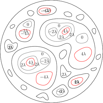
Figure 4.1: Left: A sketch of CLE₄ coupled with the GFF. The loops have boundary values $-2\lambda$ or $2\lambda$. Right: We depict a few layers of the nested CLE₄ coupled with the same GFF. We mark in red the outermost loops that have boundary values $-4\lambda$ or $4\lambda$, which belong to $\mathcal{L}_{-4\lambda,4\lambda}$.

It is also natural to consider level loops of $h$ at other heights than those of CLE₄. For example, the previous coupling can be extended to the nested CLE₄ (by sampling the CLE₄ coupled to $h^{0}|_{O(\gamma)}$ for each $\gamma\in\Gamma$), so that the further layers of CLE₄ loops are at heights $(2k+1)\lambda$ for $k\in\mathbb{Z}$. For $a\in(-\lambda,\lambda)$, the outermost level loops of $h$ at height $a$ are given by boundary conformal loop ensembles (BCLE) [MR3708206], and one can then also consider nested versions of BCLE to obtain level loops of $h$ at a continuum range of heights.

The gaskets of CLEs and BCLEs belong to a particular class of local sets called two-valued sets introduced by Aru, Sepúlveda and Werner in [MR3936643]: a two-valued set is a thin local set (a terminology in [MR4010952] meaning that the local set carries no mass of the GFF, described by (4.1)) with two boundary values in $\{-a,b\}$, denoted by $\mathbb{A}_{-a,b}$. For example, the gasket of CLE₄ is equal to $\mathbb{A}_{-2\lambda,2\lambda}$, and the gaskets of BCLEs correspond to $\mathbb{A}_{-a,b}$ with $a+b=2\lambda$. It was shown in [MR3936643] that the sets $\mathbb{A}_{-a,b}$ exist for $a,b>0$ with $a+b\geq 2\lambda$, and are a.s. unique and determined by $h$. Let us use $\mathcal{L}_{-a,b}$ to denote $\mathcal{L}(\mathbb{A}_{-a,b})$. Throughout, we denote by $\mathcal{L}^{+}_{-a,b}$ (resp. $\mathcal{L}^{-}_{-a,b}$) the set of loops in $\mathcal{L}_{-a,b}$ with boundary value $b$ (resp. $-a$). We will also use notations like CLE${}_{4}(h)$ and $\mathcal{L}_{-a,b}(h)$ to represent these sets coupled to $h$ (especially when there are different GFFs involved).

The loops in $\mathcal{L}_{-a,b}$ are composed of SLE₄-type curves which are level lines of $h$, hence are a.s. simple and do not cross each other (but can intersect each other). The law of $\mathcal{L}_{-a,b}$ is invariant under all conformal automorphisms from $D$ onto itself, since $h$ is invariant under those conformal maps. The geometric properties of the loops in $\mathcal{L}_{-a,b}$ are well understood (see e.g. [MR3936643, MR3827968, SSV] and Lemma 4.6).

Let us now give a simple and intuitive explanation of the two-valued sets, and postpone more details to the next subsection. As pointed out in [MR3936643], $\mathbb{A}_{-a,b}$ is a 2D analogue for GFF of the stopping time of a 1D Brownian motion upon exiting $[-a,b]$, and is intuitively the set of points that are connected to the boundary by a path on which the values of $h$ remain in $[-a,b]$. Let us illustrate this by the following construction of $\mathbb{A}_{-2n\lambda,2n\lambda}$ via iterated CLE₄s (see Fig. 4.1, right). For each point $z\in D$, the boundary values of the successive loops that encircle $z$ in the nested CLE₄ perform a symmetric random walk with steps $\pm 2\lambda$. The loops in $\mathcal{L}_{-2n\lambda,2n\lambda}$ correspond to the first time that we obtain a nested CLE₄ loop with boundary value equal to $-2n\lambda$ or $2n\lambda$.

Let us give more details on Gaussian free field, local sets and two-valued sets. Here, we look at a GFF in the unit disk $\mathbb{U}$. For any other simply connected domain $D$, one can simply map $D$ conformally onto $\mathbb{U}$. Let $\Gamma$ be the space of all closed nonempty subsets of $\overline{\mathbb{U}}$. We view $\Gamma$ as a metric space, endowed by the Hausdorff metric induced by the Euclidean distance. Note that $\Gamma$ is naturally equipped with the Borel $\sigma$-algebra on $\Gamma$ induced by this metric. Given $A\in\Gamma$, let $A_{\delta}$ denote the closure of the $\delta$-neighborhood of $A$ in $\mathbb{U}$. Let $\mathcal{A}_{\delta}$ be the smallest $\sigma$-algebra in which $A$ and the restriction of $h$ to the interior of $A_{\delta}$ are measurable. Let

$$\mathcal{A}:=\bigcap_{\delta\in\mathbb{Q},\delta>0}\mathcal{A}_{\delta}.$$

Intuitively, this is the smallest $\sigma$-algebra in which $A$ and the values of $h$ in an infinitesimal neighborhood of $A$ are measurable.

Definition 4.1 (Local set [MR3101840]).

Let $h$ be a GFF in $\mathbb{U}$. We say that $A$ is a local set of $h$ if $A$ is a closed subset of $\overline{\mathbb{U}}$ and one can write $h=h_{A}+h^{A}$, where

• $h_{A}$ is an $\mathcal{A}$-measurable random distribution which on $\mathbb{U}\setminus A$ a.s. has finite pointwise values and is harmonic.

• $h^{A}$ is a random distribution which is independent of $\mathcal{A}$. It is a.s. zero on $A$ and equal to an independent zero boundary GFF in each connected component of $\mathbb{U}\setminus A$.

Two-valued sets were introduced by Aru, Sepúlveda and Werner in [MR3936643]. More precisely, they denote thin local sets with two prescribed boundary values. In Section 4.1, we have mentioned the examples of CLE₄ (whose gasket is a thin local set of a GFF with two boundary values in $\{-2\lambda,2\lambda\}$) and BCLE${}_{4}(-1)$ (whose gasket is a thin local set of a GFF with two boundary values in $\{-\lambda,\lambda\}$).

In [MR3936643], the authors first defined the more general family of bounded type thin local sets (denoted by BTLS), as follows.

Definition 4.2 (Bounded type thin local sets, [MR3936643]).

Let $h$ be a GFF in $D$. Let $A$ be a relatively closed subset of $D$. For $K>0$, we say that $A$ is a $K$-BTLS of $h$ if

1. (boundedness) $A$ is a local set of $h$ such that $|h_{A}(x)|\leq K$ for all $x\in D\setminus A$.

2. (thinness) for any smooth function $f$, we have $(h_{A},f)=\int_{D\setminus A}h_{A}(x)f(x)dx$.

It was shown in [MR3936643] that a BTLS must be connected to the boundary of the domain.

Lemma 4.3 (Proposition 4, [MR3936643]).

If $A$ is a BTLS, then $A\cup\partial D$ is a.s. connected.

A two-valued set is defined to be a BTLS $A$ such that $h_{A}\in\{-a,b\}$ for $a,b>0$. The family of two-valued sets satisfies the properties of the following lemma.

Lemma 4.4 (Proposition 2 in [MR3936643]).

Let $-a<0<b$.

• When $a+b<2\lambda$, it is not possible to construct a BTLS $A$ such that $h_{A}\in\{-a,b\}$ a.s.

• When $a+b\geq 2\lambda$, there is a unique BTLS $A$ coupled with $h$ such that $h_{A}\in\{-a,b\}$ a.s. We denote this set $A$ by $\mathbb{A}_{-a,b}$.

• If $[a,b]\subseteq[a^{\prime},b^{\prime}]$, then $\mathbb{A}_{-a,b}\subseteq\mathbb{A}_{-a^{\prime},b^{\prime}}$ a.s.

This lemma shows that two-valued sets are deterministic functions of the GFF $h$ (when they exist), and this property will be instrumental in our proof.

When $a+b=2\lambda$, the set $\mathcal{L}_{-a,b}$ is equal to BCLE${}_{4}(\rho)$ and can be constructed using branching SLE${}_{4}(\rho,-2-\rho)$ processes ([MR3708206, MR3936643]). Properties of such SLE processes directly imply the following lemma.

Lemma 4.5.

If $a+b=2\lambda$, every loop in $\mathcal{L}_{-a,b}$ intersects $\partial D$.

For other values of $a,b$, $\mathbb{A}_{-a,b}$ is constructed by iterating the branching SLE${}_{4}(\rho,-2-\rho)$ processes. Properties of the SLE${}_{4}(\rho,-2-\rho)$ processes also lead to the following intersecting behavior of the loops in $\mathcal{L}_{-a,b}$.

Lemma 4.6 (Intersecting behavior of the loops [MR3827968]).

1. There exists a loop in $\mathcal{L}^{+}_{-a,b}$ (resp. $\mathcal{L}^{-}_{-a,b}$) which intersects $\partial D$ if and only if $b<2\lambda$ (resp. $a<2\lambda$).

2. If $a+b<4\lambda$, then one can connect any two loops $\eta_{1}$ and $\eta_{2}$ in $\mathcal{L}_{-a,b}$ by a finite sequence of loops $(\gamma_{1},\dots,\gamma_{n})$ so that $\gamma_{1}=\eta_{1}$, $\gamma_{n}=\eta_{2}$ and $\gamma_{k+1}$ intersects $\gamma_{k}$ for each $1\leq k\leq n-1$. Only loops with different boundary values can intersect each other.

4.2 Input from the second paper of the series

In this section we briefly recap some inputs from [DumLisQia21] that are used in this paper. We refer to [DumLisQia21] for the proofs. We only mention the main tools from [DumLisQia21] that we will use and refer, later in the proof, to the precise statements of [DumLisQia21] when they were not mentioned in this section.

Results for the double random current model

As mentioned above, we need tightness results for several families of loops, notably for the outer boundaries of the double random current clusters. This is done using an Aizenman–Burchard-type criterion for the double random current. Below, for a subset $A$ of vertices, a $A$-cluster is a cluster for the current configuration restricted to $A$. A domain $D$ is a subgraph of $\mathbb{Z}^{2}$ whose boundary is a self-avoiding polygon in $\mathbb{Z}^{2}$. Let $\Lambda_{r}:=[-r,r]^{2}$ and ${\rm Ann}(r,R):=\Lambda_{R}\setminus\Lambda_{r-1}$. Call an ${\rm Ann}(r,R)$-cluster crossing if it intersects both $\partial\Lambda_{r}$ and $\partial\Lambda_{R}$. For an integer $k\geq 1$, let $A_{2k}(r,R)$ be the event that there are $k$ distinct ${\rm Ann}(r,R)$-clusters in ${\mathbf{n}}_{1}+{\mathbf{n}}_{2}$ crossing ${\rm Ann}(r,R)$.

Theorem 4.7 (Aizenman–Burchard criterion for the double random current model).

There exist sequences $(C_{k})_{k\geq 1},(\lambda_{k})_{k\geq 1}$ with $\lambda_{k}$ tending to infinity as $k\to\infty$, such that for every domain $D$, every $k\geq 1$ and all $r,R$ with $1\leq r\leq R/2$,

$${\bf P}_{D,D}^{\emptyset,\emptyset}[A_{2k}(r,R)] \leq C_{k}(\tfrac{r}{R})^{\lambda_{k}}.$$ (4.2)

We will also need some a priori properties of possible subsequential scaling limits. These will be obtained using estimates in the discrete on certain four-arm type events. We list them now. Let

$$A_{4}^{\square}(r,R) :=\{\text{there exist two $\Lambda_{R}$-clusters crossing $\mathrm{Ann}(r,R)$}\}$$

and let $A_{4}^{\square}(x,r,R)$ be the translate of $A_{4}^{\square}(r,R)$ by $x$.

Theorem 4.8.

There exists $C>0$ such that for all $r,R$ with $1\leq r\leq R$,

$${\bf P}_{\mathbb{Z}^{2},\mathbb{Z}^{2}}^{\emptyset,\emptyset}[A_{4}^{\square}(r,R)] \leq C(r/R)^{2}.$$ (4.3)

Furthermore, for every $\varepsilon>0$, there exists $\eta=\eta(\varepsilon)>0$ such that for all $r,R$ with $1\leq r\leq\eta R$ and every domain $\Omega\supset\Lambda_{2R}$,

$${\bf P}_{\Omega,\Omega}^{\emptyset,\emptyset}[\exists x\in\Lambda_{R}:A_{4}^{\square}(x,r,R)] \leq\varepsilon.$$ (4.4)

The result is coherent with the fact that the scaling limit of the outer boundary of large clusters in ${\mathbf{n}}_{1}+{\mathbf{n}}_{2}$ is given by CLE₄, which is known to be made of simple loops that do not touch each other. Interestingly, to derive the convergence to the continuum object it will be necessary to first prove this property at the discrete level.

We turn to a second result of the same type. For a current ${\mathbf{n}}$, let ${\mathbf{n}}^{*}$ be the set of dual edges $e^{*}$ with ${\mathbf{n}}_{e}=0$. For a dual path $\gamma=(e_{1}^{*},e_{2}^{*},\dots,e_{k}^{*})$, call the ${\mathbf{n}}$-flux through $\gamma$ the sum of the ${\mathbf{n}}_{e_{i}}$. Call an ${\rm Ann}(r,R)$-hole in ${\mathbf{n}}_{1}+{\mathbf{n}}_{2}$ a connected component of $({\mathbf{n}}_{1}+{\mathbf{n}}_{2})^{*}$ restricted to ${\rm Ann}(r,R)^{*}$ (note that it can be seen as a collection of faces). An ${\rm Ann}(r,R)$-hole is said to be crossing ${\rm Ann}(r,R)$ if it intersects $\partial\Lambda_{r}^{*}$ and $\partial\Lambda_{R}^{*}$. Consider the event

$$A_{4}^{\blacksquare}(r,R) :=\Big{\{}\begin{array}[]{c}\text{there exist two ${\rm Ann}(r,R)$-holes crossing ${\rm Ann}(r,R)$ and the}\\ \text{shortest dual path between them has even $({\mathbf{n}}_{1}+{\mathbf{n}}_{2})$-flux}\end{array}\Big{\}}.$$

Denote its translate by $x$ by $A_{4}^{\blacksquare}(x,r,R)$.

Theorem 4.9.

There exists $C>0$ such that for all $r,R$ with $1\leq r\leq R$,

$${\bf P}_{\mathbb{Z}^{2},\mathbb{Z}^{2}}^{\emptyset,\emptyset}[A_{4}^{\blacksquare}(r,R)] \leq C(r/R)^{2}.$$ (4.5)

Furthermore, for every $\varepsilon>0$, there exists $\eta=\eta(\varepsilon)>0$ such that for all $r,R$ with $1\leq r\leq\eta R$ and every domain $D\supset\Lambda_{2R}$,

$${\bf P}_{\Omega,\Omega}^{\emptyset,\emptyset}[\exists x\in\Lambda_{R}:A_{4}^{\blacksquare}(x,r,R)] \leq\varepsilon.$$ (4.6)

Let us mention that the previous results are obtained using the following key statement, which is of independent interest and is also directly used in this paper. For a set $D$, let $\partial_{r}D$ be the set of vertices in $D$ that are within a distance $r$ from $\partial D$.

Theorem 4.10 (Connection probabilities close to the boundary for double random current).

There exists $c>0$ such that for all $r,R$ with $1\leq r\leq R$ and every domain $D$ containing $\Lambda_{2R}$ but not $\Lambda_{3R}$,

$$\frac{c}{\log(R/r)}\leq{\bf P}_{D,D}^{\emptyset,\emptyset}[\Lambda_{R}\stackrel{{\scriptstyle{\mathbf{n}}_{1}+{\mathbf{n}}_{2}}}{{\longleftrightarrow}}\partial_{r}D]\leq\epsilon(\tfrac{r}{R}),$$

where $x\mapsto\epsilon(x)$ is an explicit function tending to 0 as $x$ tends to 0.

We predict that the upper bound should be true for $\epsilon(x):=C/\log(1/x)$ but we do not need such a precise estimate here. Again, the result is coherent with the fact that the scaling limit of the outer boundary of large clusters in ${\mathbf{n}}_{1}+{\mathbf{n}}_{2}$ is given by CLE₄.

The lower bound is to be compared with recent estimates [DumSidTas17, DumManTas20] obtained for another dependent percolation model, namely the critical Fortuin–Kasteleyn random cluster model with cluster-weight $q\in[1,4)$. There, it was proved that the crossing probability is bounded from below by a constant $c=c(q)>0$ uniformly in $r/R$. We expect that the behaviour of the critical random cluster model with cluster weight $q=4$ on the other hand is comparable to the behaviour presented here: large clusters do not come close to the boundary of domains when the boundary conditions are free.

5 Scaling limit of the double random current clusters

In this section, we identify the scaling limit of the double random current clusters with free and wired boundary conditions. More precisely, we prove Theorems 5.1 and 5.3 which imply Theorems 1.1 and 1.2. As we have pointed out at the end of Section 1.2, Theorems 5.3 and 5.1 contain more information than Theorems 1.1 and 1.2.

Our proof crucially relies on the height function from Section 3 which satisfies a strong form of spatial Markov property at the inner boundaries of the double random current clusters, namely one has an independent height function (which converges to a GFF) inside each domain encircled by the inner boundary of a cluster. The boundary values $\sqrt{2}\lambda$ and $2\sqrt{2}\lambda$ at the inner boundaries of the clusters come from the discrete height function (in the discrete, the height changes by $\pm 1$ or $\pm 1/2$ between neighbouring sites and faces but the limiting field is $({2\sqrt{2}\lambda})^{-1}$ times the GFF, hence the values of the continuum field on the scaling limit of such inner boundaries are multiples of $\sqrt{2}\lambda$). For example, the scaling limit of the inner boundaries of the outermost cluster in a double random current model with wired boundary conditions follow directly from this spatial Markov property and the characterization of two-valued sets (Lemma 4.4) [MR3936643].

In contrast, in a double random current model with free boundary conditions, the discrete height function does not have this form of spatial Markov property at the outer boundaries of the clusters. However, we establish this spatial Markov property in the continuum limit, using additional information on the geometric properties of these loops and their interaction with other interfaces of the primal and dual models coupled through Theorem 2.1. More precisely, we show that the outer boundaries of the clusters in a free boundary double random current model converge to the CLE₄ coupled with the limiting GFF, so that each limiting loop has boundary value $-2\lambda$ or $2\lambda$. The value $2\lambda$ cannot be found in the height function of the discrete model, but only appears in the continuum limit. This is the same value as the height gap at the two sides of a level line, identified in [MR2486487] (see Remark 5.10).

Throughout, let $D\subsetneq\mathbb{C}$ be a simply connected domain whose boundary is a Jordan curve. We say that two contours $\partial U_{1}$ and $\partial U_{2}$ cross each other if $U_{1}\not\subseteq U_{2}$, $U_{2}\not\subseteq U_{1}$ and $U_{1}\cap U_{2}\not=\emptyset$. We say that a contour $\partial U_{1}$ encircles another contour $\partial U_{2}$ if $U_{2}\subseteq U_{1}$, and we say $\partial U_{1}$ strictly encircles $\partial U_{2}$ if $U_{2}\subsetneq U_{1}$.

5.1 Main results

In this section, we state the main results Theorems 5.1 and 5.3, which can be seen as enhanced versions of Theorems 1.1 and 1.2 presented in the introduction.

Free boundary conditions

Let us consider the coupling $\mathbb{P}_{D^{\delta}}$ between two independent copies ${\mathbf{n}}_{1}^{\delta}$ and ${\mathbf{n}}_{2}^{\delta}$ of sourceless currents on $D^{\delta}$, i.e., $({\mathbf{n}}_{1}^{\delta},{\mathbf{n}}_{2}^{\delta})\sim\mathbf{P}_{D^{\delta},D^{\delta}}^{\emptyset,\emptyset}$, the labels $\epsilon^{\delta}$ associated to the clusters of ${\mathbf{n}}_{1}^{\delta}+{\mathbf{n}}_{2}^{\delta}$, and the nesting field $h^{\delta}$. Let $B^{\delta}$ be the collection of outer boundaries of the outermost double random current clusters on $D^{\delta}$. For each loop $\ell\in B^{\delta}$, let $\epsilon^{\delta}(\ell)$ be the label of the double random current cluster $\mathcal{C}(\ell)$ with outer boundary $\ell$, and $A^{\delta}(\ell)$ be the collection of loops corresponding to the inner boundary of $\mathcal{C}(\ell)$. Let $A^{\delta}:=\cup_{\ell\in B^{\delta}}A^{\delta}(\ell)$. For each $\gamma\in A^{\delta}(\ell)$, we say that it is the boundary of an odd hole if $\mathcal{C}(\ell)$ is odd around every face encircled by $\gamma$ (see definition in Section 1.3). Otherwise we say that $\gamma$ is the boundary of an even hole. We let $c^{\delta}(\gamma)=1$ (resp. $c^{\delta}(\gamma)=0$) if $\gamma$ is the boundary of an odd (resp. even) hole. We will prove the following theorem.

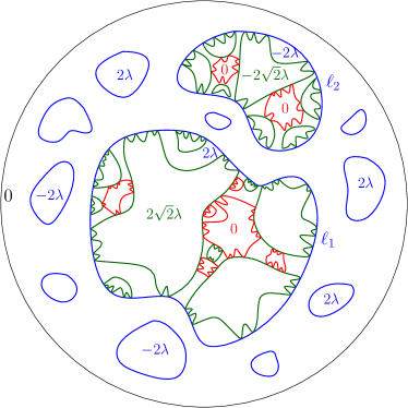
Figure 5.1: We depicted the loops in $B$ in blue. For each $\ell\in B$, the loops in $A(\ell)$ have boundary value either $0$ or $\epsilon(\ell)2\sqrt{2}\lambda$. For two loops $\ell_{1}$ and $\ell_{2}$ in $B$ with labels $\epsilon(\ell_{1})=1$ and $\epsilon(\ell_{2})=-1$, we depict the loops in $A(\ell_{1})$ and $A(\ell_{2})$. For $i=1,2$, we draw the loops in $A(\ell_{i})$ with boundary value $0$ (resp. $\epsilon(\ell_{i})2\sqrt{2}\lambda$) in red (resp. green). Each green (resp. red) loop is the limit of the boundary of an odd (resp. even) hole.

Theorem 5.1 (Free boundary conditions).

Let $D\subsetneq\mathbb{C}$ be a simply connected Jordan domain; As $\delta\to 0$, the family $(B^{\delta},A^{\delta},h^{\delta},\epsilon^{\delta},c^{\delta})$ defined above converges in distribution to a limit $(B,A,h,\epsilon,c)$ satisfying (see Fig. 5.1):

• $h$ is a GFF with zero boundary conditions in $D$.

• The collection of loops $B$ is equal to CLE${}_{4}(h)$. For each $\ell\in B$, $h|_{O(\ell)}$ is equal to an independent zero-boundary GFF $h^{0}|_{O(\ell)}$ plus the constant $\epsilon(\ell)2\lambda$.

• Every loop in $A$ is encircled by a loop in $B$. For each loop $\ell\in B$, let $A(\ell)$ denote the collection of loops in $A$ that are encircled by $\ell$.

  • If $\epsilon(\ell)=1$, then $A(\ell)$ is equal to $\mathcal{L}_{-2\lambda,(2\sqrt{2}-2)\lambda}(h^{0}|_{O(\ell)})$.

  • If $\epsilon(\ell)=-1$, then $A(\ell)$ is equal to $\mathcal{L}_{-(2\sqrt{2}-2)\lambda,2\lambda}(h^{0}|_{O(\ell)})$.

  • Each loop $\gamma\in A(\ell)$ has boundary value $\epsilon(\ell)c(\gamma)2\sqrt{2}\lambda$.

Remark 5.2.

We can deduce using crossing estimates from [DumLisQia21] that for each loop $\ell\in B$, two loops in $A(\ell)$ of the same parity (hence of the same boundary value and drawn in the same color in Fig. 5.1) never touch each other. Only the limit of odd holes can touch $\ell$. This is consistent with Theorem 5.1 and the adjacency properties of the loops in a two-valued set (Lemma 4.6). Moreover, Theorem 5.1 implies that each loop in $A(\ell)$ is connected to $\ell$ via a finite chain of loops of alternating parities (hence the length of this chain always has a fixed parity). In particular, the parity of the holes are determined by the shape of the clusters.

Theorem 5.1 implies Theorem 1.1.

Proof of Theorem 1.1.

Theorem 5.1 identifies the limit of the (inner and outer) boundaries of the outermost clusters in a double random current model with free boundary conditions. For each loop $\gamma$ in $A$, the next layer of outermost clusters in $O(\gamma)$ satisfies the same properties (i.e., Properties from Section 5.2) as the outermost clusters in $D$. The same proof as that of Theorem 5.1 then identifies the law of the next layer of outermost clusters in $O(\gamma)$. Iterating, we can deduce Theorem 1.1. ∎

Wired boundary conditions

Consider the double random current ${\mathbf{n}}$ with wired boundary conditions on the weak dual $(D^{\delta})^{\dagger}$. Let $\widehat{A}^{\delta}$ be the collection of loops in the inner boundary of the cluster $\widehat{\mathcal{C}}$ of the outer boundary of $(D^{\delta})^{\dagger}$ in ${\mathbf{n}}$. For each $\gamma\in\widehat{A}^{\delta}$, we say that it is the boundary of an odd hole if $\widehat{\mathcal{C}}$ is odd around every face encircled by $\gamma$. Otherwise we say that $\gamma$ is the boundary of an even hole. We let $\widehat{c}^{\delta}(\gamma)=1$ (resp. $\widehat{c}^{\delta}(\gamma)=-1$) if $\gamma$ is the boundary of an odd (resp. even) hole.

Below, we focus on simply connected domains $D$ with $C^{1}$-smooth boundary. The restriction to such domains comes from a technical condition from Remark 7.3 of [DumLisQia21] which could possibly be removed modulo some additional work.

Theorem 5.3 (Wired boundary conditions).

Consider a simply connected domain $D\subsetneq\mathbb{C}$ and such that $\partial D$ is $C^{1}$. Then as $\delta\to 0$, $(\widehat{A}^{\delta},h^{\delta},\widehat{c}^{\delta})$ converges in distribution to a limit $(\widehat{A},h,\widehat{c})$, where $h$ is a GFF in $D$ with zero boundary conditions and $\widehat{A}=\mathcal{L}_{-\sqrt{2}\lambda,\sqrt{2}\lambda}(h)$. Moreover, $h$ restricted to $O(\gamma)$ has boundary value $c(\gamma)\sqrt{2}\lambda$.

Remark 5.4.

We can deduce using crossing estimates from [DumLisQia21] that two loops in $\widehat{A}$ of the same parity (hence of the same boundary value and drawn in the same color in Fig. 5.2) never touch each other. This is consistent with Theorem 5.3 and the adjacency properties of the loops in a two-valued set (Lemma 4.6).

From Theorem 5.3 and Theorem 5.1 (which will be proved in the next subsection), we can deduce Theorem 1.2.

Proof of Theorem 1.2.

The first bullet point of Theorem 1.2 is given by Theorem 5.3. Given $\widehat{A}$, for each loop $\gamma\in\widehat{A}$, we have the scaling limit of an independent double random current model in $O(\gamma)$ with free boundary conditions. This Markov property together with Theorem 1.1 (which will be proved in the next subsection) implies the second and third bullet points of Theorem 1.2. ∎

5.2 First properties of the limiting interfaces

In this subsection, we first prove some properties for the free-boundary double random currents (Proposition 5.5), then prove Theorem 5.3 for the wired boundary conditions, and finally prove Lemma 5.6 which relies on the coupling of the primal and dual models.

Proposition 5.5.

Fix a simply connected Jordan domain $D\subsetneq\mathbb{C}$ and consider the double random current on $D^{\delta}$ with free boundary conditions. The family $(B^{\delta},A^{\delta},\epsilon^{\delta},h^{\delta},c^{\delta})_{\delta>0}$ is tight for the topology of weak convergence and for every subsequential limit $(B,A,\epsilon,h,c)$, a.s.

1. $h$ is a GFF with zero boundary conditions in $D$.

2. The sets $A$ and $B$ consist of simple loops which do not cross each other. Every loop in $A$ is encircled by some loop in $B$. The set $A$ is not equal to $\{\partial D\}$.

3. Almost surely, any two loops in $B$ do not intersect each other.

4. For any $z\in D$ and $R>r>0$, we say that a loop crosses the annulus $B(z,R)\setminus B(z,r)$ if it intersects both $\partial B(z,r)$ and $\partial B(z,R)$. Almost surely, there can be a finite number of loops in $B$ that cross any annulus contained in $D$.

5. (Local set) The set $\mathrm{gask}(A)$ is a thin local set of $h$ with boundary values belonging to $\{-2\sqrt{2}\lambda,0,2\sqrt{2}\lambda\}$. More precisely, for each loop $\ell\in B$, for all $\gamma\in A(\ell)$, $h$ restricted to $O(\gamma)$ is equal to an independent GFF with boundary condition $\epsilon(\ell)c(\gamma)2\sqrt{2}\lambda$.

6. The loops in $A$ that have boundary value $0$ do not touch the loops in $B$.

Proof.

Proof of tightness and Property 1. We already know that $h^{\delta}$ converges as $\delta\to 0$ to the GFF in $D$ with zero boundary conditions. Furthermore, the tightness of $\epsilon^{\delta}$ is trivial once the one of $(B^{\delta},A^{\delta})$ has been justified. We therefore focus on the latter. Recall the tightness criterion [AizBur99, H1]: a family of random variables $\mathcal{F}^{\delta}$ (with law $\mathbb{P}_{\delta}$) taking values in $\mathfrak{C}(\Omega)$ satisfies H1 if for every $k<\infty$ and every annulus $\mathrm{Ann}(x,r,R)$ with $\delta\leq r\leq R\leq 1$, the following bound holds uniformly in $\delta>0$:

$$\mathbb{P}_{\delta}[\mathrm{Ann}(x,r,R)\text{ is crossed by $k$ separate pieces of interfaces in }\mathcal{F}^{\delta}]\leq C(k)(\tfrac{r}{R})^{\lambda(k)},$$ (5.1)

with $C(k)>0$ and $\lambda(k)$ tending to infinity as $k\to\infty$.

We apply this criterion to the family $(B^{\delta}\cup A^{\delta})$ (we can also apply it to $B^{\delta}$ or $A^{\delta}$). The event that $\mathrm{Ann}(x,r,R)$ is crossed by $k$ separate pieces of interfaces in $A^{\delta}\cup B^{\delta}$ is included in the (rescaled version of the) event $A_{2k}(r/\delta,R/\delta)$, so that we may apply Theorem 4.7.

For the tightness of the $c^{\delta}$, note that $c^{\delta}$ is determined by $(A^{\delta},B^{\delta},c^{\delta})$ and the information on which holes are odd or not. The latter is determined by the odd part of the double random current, which we call $\eta^{\delta}$ for the reminder of this proof. Paper [DumLisQia21] also applies to odd parts of each currents, and therefore to the odd part of the sum, so that one may extract a converging subsequential sequence of $(\eta^{\delta})$. This concludes the proof.

Until the end of this section, consider $(B,A,\epsilon,h,c)$ to be the limit of a converging subsequence $(B^{\delta_{n}},A^{\delta_{n}},\epsilon^{\delta_{n}},h^{\delta_{n}},c^{\delta_{n}})$.

Proof of Properties 2, 3 and 4. Every loop in $A$ is surrounded by a loop in $B$ by construction. The loops in $A$ and $B$ also do not cross each other by construction.

The fact that the loops in $B$ do not intersect each other is a direct consequence of Theorem 4.8. Indeed, fix $\alpha,\beta,\varepsilon>0$. For two loops of $A^{\delta_{n}}$ of diameter at least $\alpha$ to come within distance $\beta$ of each other, there must be $x\in\Omega^{\delta_{n}}$ such that the translate by $x$ of the rescaled version of the event $A_{4}^{\square}(\beta/\delta_{n},\alpha/\delta_{n})$ occurs. Yet, Theorem 4.8 implies that provided that $\beta\leq\beta_{0}(\alpha,\varepsilon)$, this occurs with probability smaller than $\varepsilon$. The same is true for two loops of $B^{\delta_{n}}$.

The fact that the loops in $A$ and $B$ are simple is also direct consequence of Theorem 4.8. Indeed, the event that a single loop comes within distance $\beta$ of itself after going away to distance $\alpha$ also implies the same event. Letting $\beta$ tend to zero, then $\alpha$, and finally $\varepsilon$, we obtain the result.

The fact that $A$ is not equal to $\{\partial D\}$ is an easy consequence of Theorem 4.10.

Property 4 is a direct consequence of the Aizenman-Burchard criterion Theorem 4.7 given below.

Proof of Property 5. Let $\mathcal{C}(\ell)$ be the cluster whose exterior boundary is $\ell$. Notice that the definition of the nesting field implies that

$$h^{\delta_{n}}=\sum_{\ell\in B^{\delta_{n}}}\sum_{\gamma\in A^{\delta_{n}}(\ell)}(h^{\delta_{n}}_{\gamma}+\epsilon^{\delta_{n}}_{\mathcal{C}(\ell)}c^{\delta_{n}}(O(\gamma))),$$

where $h^{\delta_{n}}_{\gamma}$ is the nesting field in $O(\gamma)$. Let us start by showing that for every test function $g$,

$$\lim_{\alpha\rightarrow 0}\lim_{n\rightarrow\infty}\int_{D^{\delta_{n}}}g(x)h^{\delta_{n}}(x)\mathbf{1}_{x\in E_{\alpha}^{\delta_{n}}}dx=0,$$ (5.2)

where, if $\Lambda_{\alpha}(y):=y+[-\alpha,\alpha]^{2}$,

$$E_{\alpha}^{\delta_{n}}:=\text{ union of the $\Lambda_{\alpha}(y)$ for $y\in\alpha\mathbb{Z}^{2}$ such that $\Lambda_{2\alpha}(y)\text{ intersects some }\gamma\in A^{\delta_{n}}$}$$

(note that in particular every $x$ that is within a distance $\alpha$ of some $\gamma$ in $A^{\delta_{n}}$ must be in $E_{\alpha}^{\delta_{n}}$).

In order to prove this statement, we fix $\varepsilon>0$ and see that

$$\varepsilon\mathbb{P}_{\delta}\Big{[}\int_{D^{\delta_{n}}}g(x)h^{\delta_{n}}(x)\mathbf{1}_{x\in E_{\alpha}^{\delta_{n}}}dx\geq\varepsilon\Big{]} \leq\mathbb{E}_{\delta}\Big{[}\Big{|}\int_{D^{\delta_{n}}}g(x)h^{\delta_{n}}(x)\mathbf{1}_{x\in E_{\alpha}^{\delta_{n}}}dx\Big{|}\Big{]}$$

$$\leq\sum_{y\in\alpha\mathbb{Z}^{2}}\mathbb{E}_{\delta}\Big{[}\Big{|}\int_{\Lambda_{\alpha}(y)}g(x)h^{\delta_{n}}(x)\mathbf{1}_{x\in E_{\alpha}^{\delta_{n}}}dx\Big{|}\Big{]}$$

$$=\sum_{y\in\alpha\mathbb{Z}^{2}}\mathbb{E}_{\delta}\Big{[}1_{y\in E_{\alpha}^{\delta_{n}}}\Big{|}\int_{\Lambda_{\alpha}(y)}g(x)h^{\delta_{n}}(x)dx\Big{|}\Big{]}$$

$$\leq\sum_{y\in\alpha\mathbb{Z}^{2}}\mathbb{P}_{\delta}[y\in E_{\alpha}^{\delta_{n}}]^{1/2}\mathbb{E}_{\delta}\Big{[}\Big{(}\int_{\Lambda_{\alpha}(y)}g(x)h^{\delta_{n}}(x)dx\Big{)}^{2}\Big{]}^{1/2}$$

$$\leq\sum_{y\in\alpha\mathbb{Z}^{2}}\alpha^{c}\times C(g)\alpha^{2}\log(1/\alpha)\leq C(g,D)\log(1/\alpha)\alpha^{c}.$$

Above, we used Markov’s inequality in the first inequality, the triangle inequality in the second, the fact that $x\in E_{\alpha}^{\delta_{n}}$ is equivalent to $y\in E_{\alpha}^{\delta_{n}}$ in the third, and Cauchy–Schwarz in the fourth. In the fifth, we combine an easy estimate on the second moment of $\int_{\Lambda_{\alpha}(y)}g(x)h^{\delta_{n}}(x)dx$ based on the definition of the nesting field and RSW type estimates from [DumLisQia21], together with the fact that for $\Lambda_{\alpha}(y)$ to intersect a loop $\gamma$ in $A^{\delta_{n}}$, there must be a primal path in ${\mathbf{n}}_{1}+{\mathbf{n}}_{2}$ from $\Lambda_{\alpha}(x)$ to $\Lambda_{\beta}(x)$ or a path in $({\mathbf{n}}_{1}+{\mathbf{n}}_{2})^{*}$ from $\partial\Lambda_{\beta}(x)$ to $\partial\Lambda_{d(x,\partial D)}(x)$, where $\beta:=\sqrt{\alpha d(x,\partial D)}$.

Then, (5.2) follows by sending $n$ to infinity, then $\alpha$ to 0, and finally $\varepsilon$ to 0.

Let us recall from the proof of Property 1 that one can use the further variable $(\eta^{\delta_{n}})$. With this one at hand, we now proceed.

For every fixed $\alpha>0$, the convergence of $A^{\delta_{n}}$, the spatial Markov property (in each $O(\gamma)$, the double random current has free boundary conditions) and Theorem 1.3 imply that the functions $h^{\delta_{n}}_{\gamma}$ converge to independent GFF in $O(\gamma)$ with zero boundary conditions for every $\gamma$ with radius at least $\alpha$ (here the convergence is the convergence of the random variables obtained by averaging against a test function with compact support in $O(\gamma)$). Also, the convergence of $(B^{\delta_{n}},A^{\delta_{n}},\epsilon^{\delta_{n}},h^{\delta_{n}},c^{\delta_{n}})$ implies that the limit $h$ has the same law as

$$\sum_{\ell\in B}\sum_{\gamma\in A(\ell)}(h_{\gamma}+\epsilon_{\mathcal{C}(\ell)}c(\gamma))$$

where the $h_{\gamma}$ are independent zero-boundary GFF in each $O(\gamma)$.

Proof of Property 6. Fix $\alpha,\beta,\varepsilon>0$. For a loop of $A^{\delta_{n}}$ of diameter at least $\alpha$ and with boundary value 0 to come within a distance $\beta$ of a loop in $B^{\delta_{n}}$ of diameter at least $\alpha$, there must be $x\in\Omega^{\delta_{n}}$ such that the translate by $x$ of the rescaled version of the event $A_{4}^{\blacksquare}(\beta/\delta_{n},\alpha/\delta_{n})$ occurs. Yet, Theorem 4.9 implies that provided that $\beta\leq\beta_{0}(\alpha,\varepsilon)$, this occurs with probability smaller than $\varepsilon$. Letting $\beta$ tend to zero, then $\alpha$, and finally $\varepsilon$, we obtain the result. ∎

Proof of Theorem 5.3.

First note that the family $(\widehat{A}^{\delta},h^{\delta},\widehat{c}^{\delta})_{\delta>0}$ is tight as a consequence of Remark 7.3 of [DumLisQia21]. Let $(\widehat{A},h,\widehat{c})$ be a subsequential limit. By Theorem 5.3, we know that $h$ is a GFF with zero boundary conditions in $D$.

By the same argument as the one leading to Property 5 of Proposition 5.5, we know that $\mathrm{gask}(\widehat{A})$ is a thin local set of $h$, and that for each $\gamma\in\widehat{A}$, the restriction of $h$ to $O(\gamma)$ has boundary value equal to $\widehat{c}(\gamma)\sqrt{2}\lambda$ which is in $\{-\sqrt{2}\lambda,\sqrt{2}\lambda\}$. This uniquely characterizes $\widehat{A}$ as a two-valued set $\mathcal{L}_{-\sqrt{2}\lambda,\sqrt{2}\lambda}$, by Lemma 4.4. The reason for the difference in gaps compared to Property 5 of Proposition 5.5 comes from the construction of the nesting field in the discrete. ∎

The following lemma states how the primal double random currents are coupled with the dual ones (see Fig. 5.2). For every loop $\ell\in\widehat{A}^{\delta}$, let $B_{1}^{\delta}(\ell)$ be the collection of loops in $B^{\delta}$ which intersect $\ell$. Let $B_{1}^{\delta}$ be the union of $B_{1}^{\delta}(\ell)$ for all $\ell\in\widehat{A}^{\delta}$.

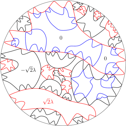
Figure 5.2: The red and black loops represent the limit of the wired d.r.c. interfaces, i.e., the loops in $\widehat{A}$. The red (resp. black) loops are the limit of even (resp. odd) holes. The blue loops are the loops in $B_{1}$.

Lemma 5.6 (Coupling with the dual d.r.c.).

The family $(B^{\delta},A^{\delta},\epsilon^{\delta},h^{\delta},\widehat{A}^{\delta},B_{1}^{\delta})_{\delta>0}$ is tight. Every subsequential limit $(B,A,\epsilon,h,\widehat{A},B_{1})$ satisfies the following properties.

• The loops in $B$ do not cross the loops in $\widehat{A}$.

• Suppose $\ell\in\widehat{A}$ has inner boundary condition $\sqrt{2}\lambda$ (resp. $-\sqrt{2}\lambda$), and let $B_{1}(\ell)$ be the set of loops in $B_{1}$ which are encircled by $\ell$. Then every loop in $B_{1}(\ell)$ has label $+1$ (resp. $-1$).

• Conditionally on $B_{1}(\ell)$, $h$ restricted to $O(\ell)\setminus(\cup_{\gamma\in B_{1}(\ell)}\overline{O}(\gamma))$ is an independent GFF with zero boundary conditions.

Proof.

Let us explain how these properties follow from the master coupling in Theorem 2.1. First of all, the fact that loops in $B$ and $\widehat{A}$ do not cross follows from Property (3) and the subsequential convergence.

Moreover, in the discrete by (2.1), the labels of the loops $\gamma\in B_{1}^{\delta}(\ell)$ are equal to the primal spin $\tau_{\mathscr{C}}$ where $\mathscr{C}$ is the cluster encircled by the loop $\gamma$ (for every $\gamma\in B_{1}^{\delta}(\ell)$, this is equal to $-1$ if the loop $\ell$ encircles an odd hole and $+1$ if it encircles and even hole), times the spin of the dual cluster of the boundary $\mathscr{C}_{\mathfrak{g}}$. By definition (1.5), the boundary conditions of the dual nesting field $h^{+}$ in $\ell$ are

$$(\tfrac{1}{2}-\mathbf{1}\{\ell\text{ encircles an odd hole}\})\tau_{\mathscr{C}_{\mathfrak{g}}}=\tfrac{1}{2}\tau_{\mathscr{C}}\tau_{\mathscr{C}_{\mathfrak{g}}}=\tfrac{1}{2}\epsilon_{\mathscr{C}}.$$

where $\epsilon_{\mathscr{C}}$ is the label of $\mathscr{C}$. By definition this is also the label of $\gamma$. Multiplying the above by $2\sqrt{2}\lambda$ and using the scaling limit of the nesting field from Theorem 1.3 gives the boundary conditions in the continuum and proves the second bullet.

Finally, in the discrete system, one can explore $O(\ell)\setminus\cup_{\ell^{\prime}\in B_{1}^{\delta}(\ell)}O(\ell^{\prime})$ from the outside, and the remaining primal double random current inside this domain has free boundary conditions. Furthermore, the corresponding primal nesting nesting field has zero boundary conditions. This follows directly from Property 2 in Theorem 2.1 and the second bullet. ∎

5.3 Proof of Theorem 5.1

In this subsection, we will prove Theorem 5.1. Suppose that $(B,A,\epsilon,h,c)$ is a subsequential limit given by Proposition 5.5, then $\mathrm{gask}(A)$ is a thin local set with boundary values in $\{-2\sqrt{2}\lambda,0,2\sqrt{2}\lambda\}$. There is a wide range of thin local sets with this property, so we need to use additional information from Section 5.2 to uniquely determine $A$. In this process, we will also uniquely determine $B$ as the CLE₄ coupled to $h$. Throughout, we let $A^{0},A^{+},A^{-}$ denote the collection of loops in $A$ that respectively have boundary value $0,2\sqrt{2}$ and $-2\sqrt{2}$.

Recall the set of loops $\widehat{A}$ defined in Theorem 5.3. Suppose that $\ell$ is a loop in $\widehat{A}$. Let $B_{1}(\ell)$ be the set of loops defined by Lemma 5.6. Let $B_{2}(\ell)$ be the set of loops which are the outer boundaries of the connected components of

$$O(\ell)\setminus(\cup_{\gamma\in B_{1}(\ell)}\overline{O}(\gamma)).$$ (5.3)

The key to the proof is the following proposition which identifies the laws of $B_{1}(\ell)$ and $B_{2}(\ell)$. See Fig. 5.3 for an illustration.

Proposition 5.7.

Suppose that $\ell\in\widehat{A}$ has boundary value $\sqrt{2}\lambda$, then

$$B_{1}(\ell)=\mathcal{L}^{+}_{-\sqrt{2}\lambda,(2-\sqrt{2})\lambda}(h^{0}|_{O(\ell)})\text{ and }B_{2}(\ell)=\mathcal{L}^{-}_{-\sqrt{2}\lambda,(2-\sqrt{2})\lambda}(h^{0}|_{O(\ell)}).$$

Otherwise if $\ell\in\widehat{A}$ has boundary value $-\sqrt{2}\lambda$, then

$$B_{1}(\ell)=\mathcal{L}^{-}_{-(2-\sqrt{2})\lambda,\sqrt{2}\lambda}(h^{0}|_{O(\ell)})\text{ and }B_{2}(\ell)=\mathcal{L}^{+}_{-(2-\sqrt{2})\lambda,\sqrt{2}\lambda}(h^{0}|_{O(\ell)}).$$

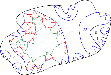
Figure 5.3: Proof of Proposition 5.7. The exterior black loop represents a loop $\ell$ in $\widehat{A}$ with boundary value $\sqrt{2}\lambda$. The blue loops represent the loops in $\mathcal{L}^{+}_{-\sqrt{2}\lambda,(2-\sqrt{2})\lambda}(h^{0}|_{O(\ell)})$ which have boundary value $2\lambda$. The complement of the blue loops constitutes the set $\mathcal{L}^{-}_{-\sqrt{2}\lambda,(2-\sqrt{2})\lambda}(h^{0}|_{O(\ell)})$ and each loop in this set has boundary value $0$. We further split each blue loop into a two-valued set with loops of boundary values $0$ (in green) and $2\sqrt{2}\lambda$ (in red). Proposition 5.7 shows that the blue loops coincide with the loops of $B_{1}(\ell)$.

In order to prove Proposition 5.7, we need to first collect a few lemmata.

Lemma 5.8.

For every $\ell\in\widehat{A}$, every loop $\eta\in B_{2}(\ell)$ touches $\ell$.

Proof.

Fix $\ell$ and $\eta$ as in the statement. To arrive at a contradiction assume that $\eta$ does not touch $\ell$. By definition of $B_{1}(\ell)$ and $B_{2}(\ell)$ this means that each point on $\eta$ must either belong to a loop in $B_{1}(\ell)$ or is approached by a sequence of loops in $B_{1}(\ell)$.

• Suppose that there is a point $z\in\eta$ which is approached by a sequence of loops in $B_{1}(\ell)$, namely there exists a sequence $(\gamma_{n})_{n\geq 0}$ of loops in $B_{1}(\ell)$ such that the distance between $z$ and $\gamma_{n}$ tends to $0$ as $n\to\infty$. Let $r>0$ be the distance between $\eta$ and $\ell$. Since each loop $\gamma_{n}$ belongs to $B_{1}(\ell)$, it must intersect $\ell$, so it must go to distance at least $r$ from $z$. On the other hand, for each $\varepsilon\in(0,r/2)$, one can find $N>0$ such that for all $n\geq N$, $\gamma_{n}$ intersects $B(z,\varepsilon)$. Therefore every loop $\gamma_{n}$ for $n\geq N$ crosses the annulus $B(z,r)\setminus B(z,\varepsilon)$, which contradicts Property 4 of Proposition 5.5. Therefore, every point on $\eta$ must belong to a loop in $B_{1}(\ell)$.

• Note that $\eta$ cannot be a subset of a single loop in $B_{1}(\ell)$, because both $\eta$ and the loops in $B_{1}(\ell)$ are simple loops so this would imply $\eta\in B_{1}(\ell)$ which is impossible.

• By the first point, there exists $\gamma\in B_{1}(\ell)$ such that $\eta\cap\gamma\not=\emptyset$. By the second point, we know that $\eta\setminus\gamma\not=\emptyset$. Let $z\in\eta\cap\gamma$ be a point which is also the limit of a sequence of points $(z_{n})_{n\geq 0}$ in the set $\eta\setminus\gamma$. By the first point, each point $z_{n}$ is on some loop in $B_{1}(\ell)$. Suppose that $\gamma_{0}\in B_{1}(\ell)$ is such that $z_{0}\in\gamma_{0}$, then $\gamma_{0}$ can only contain a finite number of points in the sequence $(z_{n})_{n\geq 0}$ because otherwise $\gamma_{0}$ would also contain the point $z$, leading to $\gamma\cap\gamma_{0}\not=\emptyset$ which contradicts Property 3 of Proposition 5.5. Let $n_{0}>0$ be the largest number such that $z_{n_{0}}\in\gamma_{0}$, then $z_{n_{0}+1}$ must be contained in a loop $\gamma_{1}\in B_{1}(\ell)$ which is different from $\gamma$ and $\gamma_{0}$. Similarly, $\gamma_{1}$ can also contain only a finite number of points in $(z_{n})_{n\geq 0}$. Iterating, we can find an infinite sequence of loops in $B_{1}(\ell)$ which approaches $z$. This contradicts the first point.

This proves the lemma. ∎

For each $\ell\in\widehat{A}$, we define the set of loops $H(\ell)$ to be the union of the loops in $B_{2}(\ell)$ together with the union of all the loops in $A$ which are encircled by some loop in $B_{1}(\ell)$. We can determine the law of $H(\ell)$.

Lemma 5.9.

For each $\ell\in\widehat{A}$, the set $H(\ell)$ is equal to $\mathcal{L}_{-\sqrt{2}\lambda,\sqrt{2}\lambda}(h^{0}|_{O(\ell)})$.

Proof.

Suppose that $\ell$ has boundary value $\sqrt{2}\lambda$ (the case where $\ell$ has boundary value $-\sqrt{2}\lambda$ is symmetric). First note that $H(\ell)$ is a set of simple loops which do not cross each other. Moreover, the gasket of $H(\ell)$ inside $O(\ell)$ is thin because it is a subset of the gasket of $A$ which is thin. By Lemma 5.6 every loop in $B_{1}(\ell)$ has label $+1$, so every loop in $A$ which is encircled by a loop in $B_{1}(\ell)$ has boundary value $2\sqrt{2}\lambda$ or $0$. Lemma 5.6 also implies that every loop in $B_{2}(\ell)$ has boundary value $0$. This uniquely determines $H(\ell)$ as a two-valued set by Lemma 4.4. ∎

By construction, the loops of $B_{1}(\ell)\cup B_{2}(\ell)$ encircle the loops of $H(\ell)$. In order to prove Proposition 5.7, it remains to understand how the loops in $B_{1}(\ell)\cup B_{2}(\ell)$ nest with the loops in $H(\ell)$. By symmetry, without loss of generality, it suffices to consider $\ell\in\widehat{A}$ with boundary value $\sqrt{2}\lambda$. We fix such a loop $\ell$ from now on until the end of the proof. Note that $H(\ell)$ is also equal to the following set of loops

$$\mathcal{L}^{-}_{-\sqrt{2}\lambda,(2-\sqrt{2})\lambda}(h^{0}|_{O(\ell)})\;\cup\bigcup_{\gamma\in\mathcal{L}^{+}_{-\sqrt{2}\lambda,(2-\sqrt{2})\lambda}(h^{0}|_{O(\ell)})}\mathcal{L}_{-2\lambda,(2\sqrt{2}-2)\lambda}(h^{0}|_{O(\gamma)}),$$

since the gasket of this set of loops forms a two-valued set with the same boundary values as $H(\ell)$. This relation describes the nesting between the loops of $H(\ell)$ and the loops of $\mathcal{L}_{-\sqrt{2}\lambda,(2-\sqrt{2})\lambda}(h^{0}|_{O(\ell)})$. We aim to show that the latter set of loops is in fact equal to $B_{1}(\ell)\cup B_{2}(\ell)$ (i.e. Proposition 5.7). Note that the loops in $\mathcal{L}_{-\sqrt{2}\lambda,(2-\sqrt{2})\lambda}(h^{0}|_{O(\ell)})$ have boundary values $0$ or $2\lambda$. Moreover, the value $2\lambda$ does not exist in the discrete height function, and only appears in the continuum limit.

Remark 5.10.

One way to see the value $2\lambda$, in the framework of our proof, is that it is the only value $a$ for which every loop in $\mathcal{L}_{-\sqrt{2}\lambda,a-\sqrt{2}\lambda}(h^{0}|_{O(\ell)})$ touches the boundary $\ell$. By definition, every loop in $B_{1}(\ell)$ touches $\ell$. We also know by Lemma 5.8 that every loop in $B_{2}(\ell)$ touches $\ell$. Consequently, if $B_{1}(\ell)\cup B_{2}(\ell)$ should be equal to a set $\mathcal{L}_{-\sqrt{2}\lambda,a-\sqrt{2}\lambda}(h^{0}|_{O(\ell)})$ (this is not a priori known, but turns out to be true), then $a$ must be equal to $2\lambda$.

More fundamentally, the value $2\lambda$ is related to the height gap at the two sides of a level line of the GFF, first identified in [MR2486487]. Suppose that we know that the loops in $B_{1}(\ell)$ are level lines of $h$ (this is not a priori known, but turns out to be true). Since we know from Lemma 5.6 that the outer sides of the loops in $B_{1}(\ell)$ (which correspond to the inner sides of the loops in $B_{2}(\ell)$) take boundary value $0$, then the inner side of the loops in $B_{1}(\ell)$ should take boundary values $-2\lambda$ or $2\lambda$.

Lemma 5.11.

We have

$$\mathcal{L}^{-}_{-\sqrt{2}\lambda,(2-\sqrt{2})\lambda}(h^{0}|_{O(\ell)})\subseteq B_{2}(\ell).$$ (5.4)

Moreover, each loop in $B_{1}(\ell)$ is encircled by a loop in $\mathcal{L}^{+}_{-\sqrt{2}\lambda,(2-\sqrt{2})\lambda}(h^{0}|_{O(\ell)})$.

Proof.

Let $\gamma$ be a loop in $\mathcal{L}^{-}_{-\sqrt{2}\lambda,(2-\sqrt{2})\lambda}(h^{0}|_{O(\ell)})$ so that $\gamma$ has boundary value $0$. By Lemma 4.5, the loop $\gamma$ a.s. intersects $\ell$. Since $\gamma$ is a $0$-loop in $H(\ell)$, it belongs either to $B_{2}(\ell)$ or $A^{0}$. Suppose that $\gamma$ belongs to $A^{0}$. Let $\gamma^{\prime}$ be the loop in $B_{1}(\ell)$ which encircles $\gamma$. Since $O(\gamma)\subseteq O(\gamma^{\prime})\subseteq O(\ell)$, we deduce that $\gamma$ must also intersect $\gamma^{\prime}$. However, by Property 6 of Proposition 5.5, we know that the loops in $A^{0}$ are disjoint from the loops in $B$, leading to a contradiction. We conclude that $\gamma$ cannot be a loop in $A^{0}$, so $\gamma$ must belong to $B_{2}(\ell)$. This implies (5.4).

Due to (5.3), each loop in $B_{1}(\ell)$ must be contained in (the closure of) a connected component of

$$O(\ell)\setminus(\cup_{\gamma\in B_{2}(\ell)}{O}(\gamma)).$$

The connected components of

$$O(\ell)\setminus(\cup_{\gamma\in\mathcal{L}^{-}_{-\sqrt{2}\lambda,(2-\sqrt{2})\lambda}(h^{0}|_{O(\ell)})}{O}(\gamma))$$

are exactly given by the domains encircled by the loops in $\mathcal{L}^{+}_{-\sqrt{2}\lambda,(2-\sqrt{2})\lambda}(h^{0}|_{O(\ell)})$. Combined with (5.4), we know that each loop in $B_{1}(\ell)$ is encircled by a loop in $\mathcal{L}^{+}_{-\sqrt{2}\lambda,(2-\sqrt{2})\lambda}(h^{0}|_{O(\ell)})$. ∎

Lemma 5.12.

For every $\xi\in\mathcal{L}^{+}_{-\sqrt{2}\lambda,(2-\sqrt{2})\lambda}(h^{0}|_{O(\ell)})$, every loop in $\mathcal{L}_{-2\lambda,(2\sqrt{2}-2)\lambda}(h^{0}|_{O(\xi)})$ is encircled by a loop in $B_{1}(\ell)$.

Proof.

Let $\xi$ be a loop in $\mathcal{L}^{+}_{-\sqrt{2}\lambda,(2-\sqrt{2})\lambda}(h^{0}|_{O(\ell)})$ and let $\eta$ be a loop in $\mathcal{L}_{-2\lambda,(2\sqrt{2}-2)\lambda}(h^{0}|_{O(\xi)})$. Then $\eta$ has boundary value either $0$ or $2\sqrt{2}\lambda$. If $\eta$ has boundary value $2\sqrt{2}\lambda$, then since $\eta\in H(\ell)$, we know that $\eta\in A^{+}$ and $\eta$ must be encircled by some loop in $B_{1}(\ell)$. We now suppose that $\eta$ has boundary value $0$, and we will show that $\eta$ must belong to $A^{0}$ and be encircled by some loop in $B_{1}(\ell)$. Indeed, note that $\eta\in\mathcal{L}^{-}_{-2\lambda,(2\sqrt{2}-2)\lambda}(h^{0}|_{O(\xi)})$. By Lemma 4.6, $\eta$ must not intersect $\xi$, hence $\eta$ also does not intersect $\ell$. Suppose by contradiction that $\eta$ is not encircled by any loop in $B_{1}(\ell)$, then $\eta$ must belong to $B_{2}(\ell)$. However, by Lemma 5.8 every loop in $B_{2}(\ell)$ intersects $\ell$ which is a contradiction. We ultimately conclude that $\eta$ is encircled by a loop in $B_{1}(\ell)$. ∎

We are now ready to prove Proposition 5.7.

Proof of Proposition 5.7.

Suppose that $\xi$ is a loop in $\mathcal{L}^{+}_{-\sqrt{2}\lambda,(2-\sqrt{2})\lambda}(h^{0}|_{O(\ell)})$. Lemma 5.12 implies that every loop in $\mathcal{L}_{-2\lambda,(2\sqrt{2}-2)\lambda}(h^{0}|_{O(\xi)})$ is encircled by a loop in $B_{1}(\ell)$, which should itself be encircled by $\xi$ by Lemma 5.11. Note that the gasket of $\mathcal{L}_{-2\lambda,(2\sqrt{2}-2)\lambda}(h^{0}|_{O(\xi)})$ in $O(\xi)$ is thin in the sense of Definition 4.2, so in particular this gasket cannot contain any open ball. Every point in $\overline{O}(\xi)$ is either encircled by a loop in $\mathcal{L}_{-2\lambda,(2\sqrt{2}-2)\lambda}(h^{0}|_{O(\xi)})$, or is equal to the limit of a sequence of points which are each encircled by some loop in $\mathcal{L}_{-2\lambda,(2\sqrt{2}-2)\lambda}(h^{0}|_{O(\xi)})$. As a consequence, there exists a set of loops $U(\xi)\subseteq B_{1}(\ell)$ which are all encircled by $\xi$ such that

$$\overline{O}(\xi)=\overline{\cup_{\gamma\in U(\xi)}O(\gamma)}.$$ (5.5)

Now, let us show that $\xi$ in fact belongs to $B_{1}(\ell)$, namely $U(\xi)$ contains only one loop which is $\xi$. If this is not the case, then there exists a loop $\gamma_{1}\in U(\xi)$ which is not equal to $\xi$. This implies that there exists a point $z\in\gamma_{1}\setminus\xi$. Since $O(\gamma_{1})\subseteq O(\xi)$, we have $z\in O(\xi)$. Due to (5.5) and Property 3 of Proposition 5.5, $z$ must be approached by a sequence of loops in $U(\xi)$. Since $z$ is at positive distance from $\ell$ and every loop in $U(\xi)$ intersects $\ell$, this also creates an infinite sequence of loops that cross an annulus around $z$, which contradicts Property 4 of Proposition 5.5. This proves that $\xi\in B_{1}(\ell)$. Therefore

$$\mathcal{L}^{+}_{-\sqrt{2}\lambda,(2-\sqrt{2})\lambda}(h^{0}|_{O(\ell)})\subseteq B_{1}(\ell).$$ (5.6)

Note that $B_{1}(\ell)\cup B_{2}(\ell)$, as well as $\mathcal{L}_{-\sqrt{2}\lambda,(2-\sqrt{2})\lambda}$, is a set of simple loops which do not cross or nest with each other and whose gasket is thin in $O(\ell)$. Therefore, the $\subseteq$ in (5.4) and (5.6) should be equalities, since there can be no other loop in $B_{1}(\ell)\cup B_{2}(\ell)$ apart from those in $\mathcal{L}_{-\sqrt{2}\lambda,(2-\sqrt{2})\lambda}$. This completes the proof of the proposition. ∎

We are now ready to prove Theorem 5.1.

Proof of Theorem 5.1.

Proposition 5.7 implies that the gasket of the following set of loops

$$B_{0}:=\bigcup_{\ell\in\widehat{A}}B_{1}(\ell)\cup B_{2}(\ell)$$

is a thin local set of $h$ with boundary values in $\{-2\lambda,0,2\lambda\}$. Moreover, every loop $\gamma$ in $\bigcup_{\ell\in\widehat{A}}B_{1}(\ell)$ has boundary value $2\lambda\epsilon(\gamma)$, and the loops in $\bigcup_{\ell\in\widehat{A}}B_{2}(\ell)$ have boundary value $0$. The union of the loops in $\bigcup_{\ell\in\widehat{A}}B_{1}(\ell)$ together with the union of $\mathcal{L}_{-2\lambda,2\lambda}(h^{0}|_{O(\gamma)})$ over all loops $\gamma\in\bigcup_{\ell\in\widehat{A}}B_{2}(\ell)$ forms a thin local set of $h$ with boundary values in $\{-2\lambda,2\lambda\}$, hence must be equal to CLE${}_{4}(h)$. This implies that for every $\ell\in\widehat{A}$, every loop in $B_{1}(\ell)$ is a loop in CLE${}_{4}(h)$.

On the other hand, for every $\ell\in\widehat{A}$ and every $\gamma\in B_{2}(\ell)$, we again have the scaling limit of an independent double random current in $O(\gamma)$. The height function of this double random current model is equal to an independent zero-boundary GFF in $O(\gamma)$. We can apply the same reasoning to the model in $O(\gamma)$ and deduce that the following set of loops

$$\bigcup_{\ell\in\mathcal{L}^{+}_{-\sqrt{2}\lambda,\sqrt{2}\lambda}(h|_{O(\gamma)})}\mathcal{L}^{+}_{-\sqrt{2}\lambda,(2-\sqrt{2})\lambda}(h^{0}|_{O(\ell)})\;\cup\bigcup_{\ell\in\mathcal{L}^{-}_{-\sqrt{2}\lambda,\sqrt{2}\lambda}(h|_{O(\gamma)})}\mathcal{L}^{-}_{(\sqrt{2}-2)\lambda,\sqrt{2}\lambda}(h^{0}|_{O(\ell)})$$

all belong to $B$ and also belong to CLE${}_{4}(h)$. Iterating, we can deduce that $B$ is in fact equal to CLE${}_{4}(h)$, and every loop $\gamma\in B$ has boundary value $2\lambda\epsilon(\gamma)$. The loops in $A(\gamma)$ is a thin local set of $h^{0}|_{O(\gamma)}$ with two boundary values, hence is uniquely determined by Lemma 4.4. Property 5 further implies that a loop in $A$ has the right boundary value as stated in Theorem 5.1. This completes the proof. ∎

5.4 Asymptotic behavior of the number of clusters

Let us now prove a lemma which leads to the asymptotic numbers of clusters in the double random current models that surround the origin.

Lemma 5.13.

In the scaling limit of the double random current model in the unit disk (with either the free or wired boundary conditions), let $N(\varepsilon)$ be the number of clusters surrounding the origin such that their outer boundaries have a conformal radius w.r.t. the origin at least $\varepsilon$. Then

$$N(\varepsilon)/\log(\varepsilon^{-1})\underset{\varepsilon\to 0}{\longrightarrow}1/(\sqrt{2}\pi^{2}).$$

Proof.

By Theorems 1.1 and 1.2 and [MR3936643, Proposition 20], we know that the difference of log conformal radii between the outer boundaries of two successive double random current clusters that encircle the origin is given by $R:=T_{1}+T_{2}$, where $T_{1}$ is the first time that a standard Brownian motion exits $[-\pi,(\sqrt{2}-1)\pi]$ and $T_{2}$ is the first time that a standard Brownian motion exits $[-\pi,\pi]$. We have

$$\mathbb{E}(T_{1}+T_{2})=(\sqrt{2}-1)\pi^{2}+\pi^{2}=\sqrt{2}\pi^{2}.$$

The $n$-th cluster which encircles the origin has log conformal radius equal to $-S_{n}$ where $S_{n}:=-(R_{1}+\cdots+R_{n})$ and $R_{i}$ are i.i.d. random variables distributed like $R$. Then $N(\varepsilon)$ is the smallest $n\geq 1$ such that $S_{n+1}\geq\log(\varepsilon^{-1})$. By the law of large numbers, we know that $S_{n}/n$ converges to $\mathbb{E}(R)$ a.s. as $n\to\infty$. Since $N(\varepsilon)\to\infty$ as $\varepsilon\to 0$, we also have that

$$S_{N(\varepsilon)+1}/(N(\varepsilon)+1)\to\mathbb{E}(R)\text{ a.s. as }\varepsilon\to 0.$$

Note that $\log(\varepsilon^{-1})\leq S_{N(\varepsilon)+1}\leq\log(\varepsilon^{-1})+R_{N(\varepsilon)}$. It follows that

$$\lim_{\varepsilon\to 0}\log(\varepsilon^{-1})/N(\varepsilon)=\mathbb{E}(R)=\sqrt{2}\pi^{2}.$$

The inverse of the above equation proves the lemma. ∎