Adaptive Denoising via GainTuning
Abstract
Deep convolutional neural networks (CNNs) for image denoising are usually trained on large datasets. These models achieve the current state of the art, but they have difficulties generalizing when applied to data that deviate from the training distribution. Recent work has shown that it is possible to train denoisers on a single noisy image. These models adapt to the features of the test image, but their performance is limited by the small amount of information used to train them. Here we propose “GainTuning”, in which CNN models pre-trained on large datasets are adaptively and selectively adjusted for individual test images. To avoid overfitting, GainTuning optimizes a single multiplicative scaling parameter (the “Gain”) of each channel in the convolutional layers of the CNN. We show that GainTuning improves state-of-the-art CNNs on standard image-denoising benchmarks, boosting their denoising performance on nearly every image in a held-out test set. These adaptive improvements are even more substantial for test images differing systematically from the training data, either in noise level or image type. We illustrate the potential of adaptive denoising in a scientific application, in which a CNN is trained on synthetic data, and tested on real transmission-electron-microscope images. In contrast to the existing methodology, GainTuning is able to faithfully reconstruct the structure of catalytic nanoparticles from these data at extremely low signal-to-noise ratios.
1 Introduction
Like many problems in image processing, the recovery of signals from noisy measurements has been revolutionized by the development of convolutional neural networks (CNNs) [65, 8, 66]. These models are typically trained on large databases of images, either in a supervised [37, 65, 8, 67, 66] or an unsupervised fashion [61, 3, 27, 29]. Once trained, these solutions are evaluated on noisy test images. This approach achieves state-of-the-art performance when the test images and the training data belong to the same distribution. However, when this is not the case, the performance of these models is often substantially degraded [58, 37, 67]. This is an important limitation for many practical applications, in which it is challenging (or even impossible) to gather a training dataset that is comparable in noise and signal content to the images encountered at test time. Overcoming this limitation requires adaptation to the test data.
A recent unsupervised method (Self2Self) has shown that CNNs can be trained exclusively on individual test images, producing impressive results [46]. Self2Self adapts to the test image, but its performance is limited by the small amount of information available for learning. As a result it generally underperforms CNN models trained on large databases.
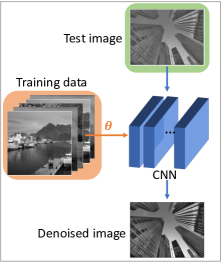
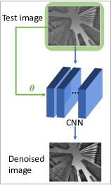
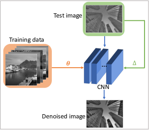
In this work, we propose GainTuning, a framework to bridge the gap between models trained on large datasets without adaptation, and models trained exclusively on test images. In the spirit of two recent methods [54, 58], GainTuning adapts pre-trained CNN models to individual test images by minimizing an unsupervised denoising cost function, thus fusing the generic capabilities obtained from the training data with specific refinements matched to the structure of the test data. GainTuning does not adapt the full parameter set (filter weights and additive constants) to the test image, but instead optimizes a single multiplicative scaling parameter (the “Gain”) for each channel within each layer of the CNN. The dimensionality of this reduced parameter set is a small fraction () of that of the full parameter set. We demonstrate through extensive examples that this prevents overfitting to the test data. The GainTuning procedure is general, and can be applied to any CNN denoising model, regardless of the architecture or pre-training process.
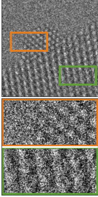
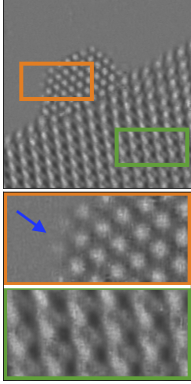
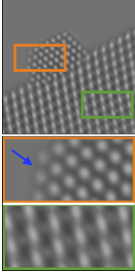
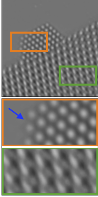
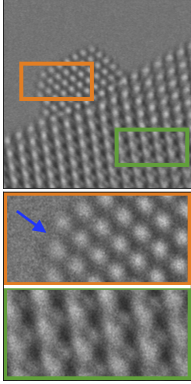
Our contributions. GainTuning provides a novel method for adapting CNN denoisers trained on large datasets to a single test image. GainTuning improves state-of-the-art CNNs on standard image-denoising benchmarks, boosting their denoising performance on nearly every image in held-out test sets. Performance improvements are even more substantial when the test images differ systematically from the training data. We showcase this ability through controlled experiments in which we vary the distribution of the noise and image structure of the test data. Finally, we evaluate GainTuning in a real scientific-imaging application where adaptivity is crucial: denoising transmission-electron-microscope data at extremely low signal-to-noise ratios. As shown in Figure 2, both CNNs pre-trained on simulated images and CNNs trained only on the test data produce denoised images with substantial artefacts. In contrast, GainTuning achieves effective denoising, accurately revealing the atomic structure in the real data.
| (a) Pre-training on a database | (b) Adaptive training on test image | (c) Combined pre-training and test-adaptive training |
 |
 |
 |
| (a) Noisy image | (b) Unsupervised training only on (a) [46] | (c) Supervised training on simulated data [38] | (d) GainTuning on CNN trained on sim. data (c) | (e) Estimated reference image |
|---|---|---|---|---|
 |
 |
 |
 |
 |
2 Related Work
Denoising via deep learning. In the last five years, CNN-based methods have clearly outperformed prior state of the art [13, 52, 6, 45, 14, 21, 10]. Denoising CNNs are typically trained in a supervised fashion, minimizing mean squared error between (MSE) over a large database of example ground-truth images and their noisy counterparts [65, 37, 8]. Unsupervised denoising is an alternative approach, which does not rely on ground-truth clean images. There are two main strategies to achieve this: blind-spot methods [27, 29, 3, 61] and techniques based on Stein’s unbiased risk estimator (SURE) [13, 33, 48, 36, 54, 55] (see Section 4 for a more detailed description).
Generalization to out-of-distribution images. In order to adapt CNNs to operate on test data with characteristics differing from the training set, recent publications propose fine-tuning the networks using an additional training dataset that is more aligned with the test data [58, 18]. This is a form of transfer learning, a popular technique in classification problems [12, 63]. However, it is often challenging to obtain relevant additional training data. Here, we show that GainTuning can adapt CNN denoisers using only the test image.
Connection to feature normalization in CNNs. Feature normalization techniques such as batch normalization (BN) [23] are a standard component of deep CNNs. BN consists of two stages: (1) centering and normalizing the features corresponding to each channel, (2) scaling and shifting the normalized features using two learned parameters per channel (a scaling factor and a shift). The scaling parameter is analogous to the gain parameter introduced in GainTuning. However, in BN this parameter is fixed during test time, whereas GainTuning explicitly adjusts it based on the test data.
Gain normalization. Motivated by normalization observed in biological sensory neurons [5], adaptive normalization of channel gains has been previously applied in object recognition [24], density estimation [1], and compression [2]. In contrast to these approaches, which adjust gains based on channel responses, GainTuning adjusts them to optimize an unsupervised cost function.
Adapting CNN denoisers to test data. To the best of our knowledge, adaptation of CNN denoisers to test data was pioneered by [55, 58]. Ref. [55] proposes to include the noisy test images in the training set. In a recent extension, the authors propose fine-tuning all the parameters in a pre-trained CNN on a single test image using the SURE cost function [54]. Ref. [58] proposes to do the same using a novel cost function based on noise resampling (see Section 4 for a detailed description). As shown in Section E fine-tuning all the parameters in a denoiser using only a single test image can lead to overfitting. Ref. [54] avoids this using early stopping, selecting the number of fine-tuning steps beforehand. Ref. [58] uses a specialized architecture with a reduced number of parameters. Here, we propose a framework for adaptive denoising that generalizes these previous methods. We show that several unsupervised cost functions can be used to perform adaptation without overfitting, as long as we only optimize a subset of the model parameters (the gain of each channel).
Adjustment of channel parameters to improve generalization in other tasks. Adjustment of channel parameters, such as gains and biases, has been shown to improve generalization in multiple machine-learning tasks, such as the vision-language problems [43, 11], image generation [7], style transfer [17], and image restoration [20]. In these methods, the adjustment is carried out while training the model by minimizing a supervised cost function. In image classification, recent studies have proposed performing adaptive normalization [25, 41, 50] and optimization [60] of channel parameters during test time, in the same spirit as GainTuning.
3 Proposed Methodology: GainTuning
In this section we describe the GainTuning framework. Let be a CNN denoiser parameterized by weight and bias parameters, . We assume that we have available a training database and a test image that we aim to denoise. First, the networks parameters are optimized on the training database
| (1) |
The cost function used for pre-training can be supervised, if the database contains clean and noisy examples, or unsupervised, if it only contains noisy data.
A natural approach to adapt the pre-trained CNN to the test data is to finetune all the parameters in the CNN, as is done in all prior works on test-time adaptation [58, 54, 18]. Unfortunately this can lead to overfitting the test data (see Section E). Due to the large number of degrees of freedom, the model is able to minimize the unsupervised cost function without denoising the noisy test data effectively. This can be avoided to some extent by employing CNN architectures with a small number of parameters [58], or by only optimizing for a short time (“early stopping”) [54]. Unfortunately, using a CNN with reduced parameters can limit performance (see Section 5), and it is unclear how to choose a single criterion for early stopping that can operate correctly for each individual test image. Here, we propose a different strategy: tuning a single parameter (the gain) in each channel of the CNN. GainTuning can be applied to any pre-trained CNN.
We denote the gain parameter of a channel in a particular layer by , and the parameters of that channel by (this is a vector that contains the weight and bias filter parameters). We define the GainTuning parameters as
| (2) |
We estimate the gains by minimizing an unsupervised loss that only depends on the noisy image:
| (3) |
The final denoised image is . Section 4 describes several possible choices for the cost function . Since we use only one scalar parameter per channel, the adjustment performed by GainTuning is very low-dimensional ( of the dimensionality of ). This makes optimization quite efficient, and prevents overfitting (see Section E).
4 Cost Functions for GainTuning
A critical element of GainTuning is the use of an unsupervised cost function, which is minimized in order to adapt the pre-trained CNN to the test data. Here, we describe three different choices, each of which are effective when integrated in the GainTuning framework, but which have different benefits and limitations.
Blind-spot loss. This loss measures the ability of the denoiser to reproduce the noisy observation, while excluding the identity solution. To achieve this, the CNN must estimate the th pixel of the noisy image as a function of the other pixels , but excluding the pixel itself. As long as the noise degrades pixels independently, this will force the network to learn a nontrivial denoising function that exploits the relationships between pixels that are present in the underlying clean image(s). The resulting loss can be written as
| (4) |
Here the expectation is over the data distribution and the selected pixel. We have slightly abused notation to indicate that the network does not use . This “blind spot” can be enforced through architecture design [29], or by masking [3, 27] (see also [46] and [61] for related approaches). The blind-spot loss has a key property that makes it very powerful in practical applications: it makes no assumption about the noise distribution (other than pixel-wise independence). When combined with GainTuning it achieves effective denoising of real electron-microscope data at very low SNRs (see Figure 2 and Section 5.4, F.5).
Stein’s Unbiased Risk Estimator (SURE). Let be an -dimensional ground-truth random vector and let be a corresponding noisy observation, where . SURE provides an expression for the MSE between and a denoised estimate , which only depends on the noisy observation :
| (5) |
The last term in Equation 8 is the divergence of , which can be approximated using Monte Carlo techniques [47] (Section D). The divergence is the sum of the partial derivatives of each denoised pixel with respect to the corresponding input pixel. Intuitively, penalizing it forces the denoiser to not rely as heavily on the th noisy pixel to estimate the th clean pixel. This is similar to the blind-spot strategy, with the added benefit that the th noisy pixel is not ignored completely. To further illustrate this connection, consider a linear convolutional denoising function , where the center-indexed parameter vector is . The SURE cost function (Equation 8) reduces to
| (6) |
The SURE loss equals the MSE between the denoised output and the noisy image, with a penalty on the “self” pixel. As this penalty is increased, the self pixel will be ignored, so the loss tends towards the blind-spot cost function. When integrated in the GainTuning framework, the SURE loss achieves effective denoising in the case of additive Gaussian noise, outperforming the blind-spot loss.
Noise Resampling. Ref. [58] introduced a novel procedure for adaptation which we call noise resampling. Given a pre-trained denoiser and a test image , first we obtain an initial denoised image by applying to , . Then we artificially corrupt by simulating noise from the same distribution as the data of interest to create synthetic noisy examples. Finally, the denoiser is fine-tuned by minimizing the MSE between and the synthetic examples. If we assume additive noise, the resulting loss is of the form
| (7) |
Noise resampling is reminiscent of Refs. [40, 62], which add noise to an already noisy image. When integrated in the GainTuning framework, the noise-resampling loss results in effective denoising in the case of additive Gaussian noise, although it tends to underperform the SURE loss.
5 Experiments and Results
In order to evaluate the performance of GainTuning we performed three different types of experiment: In-distribution (test examples held out from the training set); out-of-distribution noise (noise level or distribution differs between training and test examples); and out-of-distribution signal (clean images drawn from a different set than the training set). We also apply GainTuning to real data from a transmission electron microscope.
Our experiments make use of four datasets: The BSD400 natural image database [34] with test sets Set12 and Set68 [65], the Urban100 images of urban environments [22], the IUPR dataset of scanned documents [4], and a set of synthetic piecewise constant images [31] (see Section B). We demonstrate the broad applicability of GainTuning by using it in conjunction with multiple architectures for image denoising: DnCNN [65], BFCNN [37], UNet [49] and Blind-spot net [29] (see Section A). Finally, we compare our results to several baselines: (1) models trained on the training database, (3) CNN models adapted by fine-tuning all parameters (as opposed to just the gains), (3) a model trained only on the test data, (4) LIDIA, a specialized architecture and adaptation strategy proposed in [58]. We provide details on training and optimization in Section C.
| Model Set12 BSD68 GainTuning DnCNN Pre-trained 29.52 28.21 27.19 28.39 27.16 26.27 GainTuning 29.62 28.30 27.29 28.47 27.23 26.33 UNet Pre-trained 29.34 28.05 27.05 28.27 27.05 26.15 GainTuning 29.46 28.15 27.13 28.34 27.12 26.22 Baseline LIDIA Pre-trained 29.46 27.95 26.58 28.24 26.91 25.74 Adapted 29.50 28.10 26.95 28.23 26.97 26.02 Self2Self 29.21 27.80 26.58 27.83 26.67 25.73 |
|
5.1 GainTuning surpasses state-of-the-art performance for in-distribution data
Experimental set-up. We use BSD400, a standard natural-image benchmark, corrupted with Gaussian white noise with standard deviation sampled uniformly from (relative to pixel intensity range ). Following [65], we evaluate performance on two independent test sets: Set12 and BSD68, corrupted with Gaussian noise with .
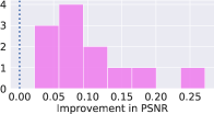
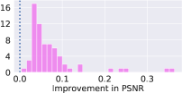
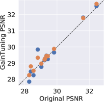
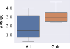
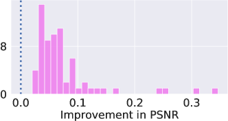
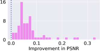
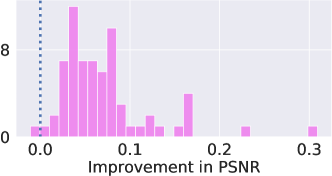
Comparison to pre-trained CNNs. GainTuning consistently improves the performance of pre-trained CNN models. Figure 3 shows this for two different models, DnCNN [65] and UNet [49] (see also Section F.1). The SURE loss outperforms the blind-spot loss, and is slightly better than noise resampling (Table 5). The same holds for other architectures, as reported in Section F.1. On average the improvement is modest, but for some images it is quite substantial (up to 0.3 dB in PSNR for , see histogram in Figure 3).
Comparison to other baselines. GainTuning outperforms fine-tuning based on optimizing all the parameters for different architectures and loss functions (see Section E). GainTuning clearly outperforms a Self2Self model, which is trained exclusively on the test data (Figure 3). It also outperforms the specialized architecture and adaptation process introduced in [58], with a larger gap in performance for higher noise levels.
5.2 GainTuning generalizes to new noise distributions
Experimental set-up. The same set-up as Section 5.1 is used, except that the test sets are corrupted with Gaussian noise with (recall that training occurs with ).
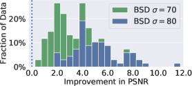
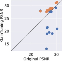
Comparison to pre-trained CNNs. Pre-trained CNN denoisers fail to generalize in this setting. GainTuning consistently improves their performance (see Figure 4 and).
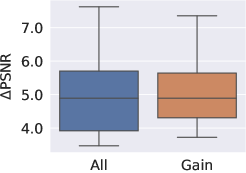
The SURE loss again outperforms the blind-spot loss, and is slightly better than noise resampling (see Section F.2). The same holds for other architectures, as reported in Section F.2. The improvement in performance for all images is substantial (up to 12 dB in PSNR for , see histogram in Figure 4).
Comparison to other baselines. GainTuning achieves comparable performance to a gold-standard CNN trained with supervision at all noise levels (Figure 4). GainTuning matches the performance of a bias-free CNN [37] specifically designed to generalize to out-of-distribution noise (Figure 4). GainTuning outperforms fine-tuning based on optimizing all the parameters for different architectures and loss functions (see Section E). GainTuning clearly outperforms a Self2Self model trained exclusively on the test data (Section F.2), and the LIDIA adaptation method [58].
| Out-of-distribution test noise | ||
| Test set Trained on Bias Free Model [37] Trained on Pre-trained Gaintuning Set12 22.45 25.54 25.59 25.50 18.48 24.57 24.94 24.88 BSD68 22.15 24.89 24.87 24.88 18.72 24.14 24.38 24.36 |
|
|
| Out-of-distribution test image | ||
| Training data Test data Pre-trained Gaintuning (a) Piecewise constant Natural images 27.31 28.60 (b) Natural images Urban images 28.35 28.79 (c) Natural images Scanned documents 30.02 30.73 |
|
|
5.3 GainTuning generalizes to out-of-distribution image content
Experimental set-up. We evaluate the performance on of GainTuning on test images that have different characteristics from the training images. We perform the following controlled experiments:
-
(a) Simulated piecewise constant images Natural images. We pre-train CNN denoisers on simulated piecewise constant images. These images consists of constant regions (of different intensities values) with the boundaries having varied shapes such as circle and lines with different orientations (see Section B for some examples). Piecewise constant images provide a crude model for natural images [35, 44, 31]. We use GainTuning to adapt a CNN trained on this dataset to generic natural images (Set12). This experiment demonstrates the ability of GainTuning to adapt from a simple simulated dataset to a significantly more complex real dataset.
-
(b) Generic natural images Images with high self-similarity. We apply GainTuning to adapt a CNN trained on generic natural images to images in Urban100 dataset. Urban100 consists of images of buildings and other structures typically found in an urban setting, which contain substantially more repeating/periodic structure (see Section B) than generic natural images.
-
(c) Generic natural images Images of scanned documents. We apply GainTuning to adapt a CNN trained on generic natural images to images of scanned documents in IUPR dataset (see Section B).
All CNNs were trained for denoising Gaussian white noise with standard deviation and evaluated at .
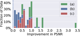
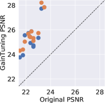
Comparison to pre-trained CNNs. GainTuning consistently improves the performance of pre-trained CNNs in all the three experiments. Figure 4 shows this for DnCNN when GainTuning is based on SURE loss. We obtain similar results with other architectures (see Section F.3). In experiment (a), all test images show substantial improvements, with one image improving as much as 3 dB in PNSR (at ). We observe similar trends for experiments (b) and (c) as well, with improvements being better on an average for experiment (c). Note that we obtain similar performance increases when both image and noise are out-of-distribution as discussed in Section F.4.
Comparison to other baselines. Experiment (a): (1) GainTuning outperforms optimizing all the parameters over different architectures and loss functions for experiment (Section E). (2) Self2Self trained only on test data outperforms GainTuningin these cases, even though GainTuning improves the performance of pre-trained CNN about 1.3 dB on an average. This is because the test images contain content that differs substantially from the training images. Self2Self provides the strongest form of adaptation, since it is trained exclusively on the test image, whereas the denoising properties of GainTuning are partially due to the pretraining (see Sections 7, F.3). (3) We did not evaluate LIDIA [58] for this experiment. Experiments (b) and (c). (1) Training all parameters clearly outperforms GainTuning for case (b), but has similar performance for (c). GainTuning outperforms LIDIA on experiments (b) and (c). Self2Self trained exclusively on test data outperforms GainTuning(and LIDIA) on (b) and (c) (see Sections 7, F.3).
5.4 Application to Electron microscopy
Scientific motivation. Transmission electron microscopy (TEM) is a popular imaging technique in materials science [53, 57]. Recent advancements in TEM enable to image at high frame rates [16, 15]. These images can for example capture the dynamic, atomic-level rearrangements of catalytic systems [56, 19, 30, 32, 9], which is critical to advance our understanding of functional materials. Acquiring image series at such high temporal resolution produces data severely degraded by shot noise. Consequently, there is an acute need for denoising in this domain.
The need for adaptive denoising. Ground-truth images are not available in TEM, because measuring at high SNR is often impossible. Prior works have addressed this by using simulated training data [38, 59], whereas others have trained CNNs directly on noisy real data [51].
Dataset. We use the training set of simulated images and the test set of 40 real TEM images from [38, 59]. The data correspond to a catalytic platinum nanoparticle on a CeO2 support (Section B).
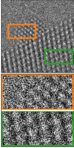
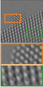
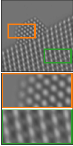
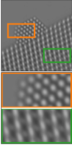
Comparison to pre-trained CNN. A CNN [29] pre-trained on the simulated data fails to reconstruct the pattern of atoms faithfully (green box in Figure 2 (c), (e)). GainTuning applied to this CNN using the blind-spot loss correctly recovers this pattern (green box in Figure 2 (d), (e)) reconstructing the small oxygen atoms in the CeO2 support. GainTuning with noise resampling failed to reproduce the support pattern (probably because it is absent from the initial denoised estimate) (Section F.5).
Comparison to other baselines. GainTuning clearly outperforms Self2Self, which is trained exclusively on the real data. The denoised image from Self2Self shows missing atoms and substantial artefacts (see Section F.5). We also compare GainTuning dataset to blind-spot methods using the 40 test frames [29, 51]. GainTuning clearly outperforms these methods (see Section F.5). Finally, GainTuning outperforms fine-tuning based on optimizing all the parameters, which overfits heavily (see Section E).
| (a) Noisy image | (b) Trained on piecewise constant | (c) After GainTuning on (b) | (d) Difference b/w (b) and (c) |
 |
 |
 |
 |
| Noisy | Before GT | Filter bef. | After GT | Filter af. | Noisy | Before GT | Filter bef | After GT | Filter af. |
|---|
6 Analysis
In this section, we perform a qualitative analysis of the properties of GainTuning.
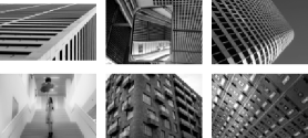
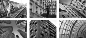
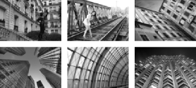
What kind of images benefit the most from adaptive denoising? Section G.1 shows the images in the different test datasets for which GainTuning achieves the most and the least improvement in PSNR. For different architecture, the result is quite consistent: GainTuning is more beneficial for images with highly repetitive patterns. This makes intuitive sense; the repetitions effectively provide multiple examples from which to learn these patterns during the unsupervised refinement.
Generalization via GainTuning. Section G.2 shows that GainTuning can achieve generalization to images that are similar to the test image used for adaptation.
How does GainTuning adapt to out-of-distribution noise? Generalization to out-of-distribution noise provides a unique opportunity to understand how GainTuning modifies the denoising function. Ref. [37] shows that the first-order Taylor approximation of denoising CNNs trained on multiple noise levels tend to have a negligible constant term, and that the growth of this term is the primary culprit for the failure of these models when tested on new noise levels. GainTuning reduces the amplitude of this constant term, facilitating generalization (See Section G.3 for more details).
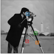
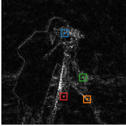
How does GainTuning adapt to out-of-distribution images? Figure 5 shows the result of applying a CNN trained on piecewise-constant images to natural images. Due to its learned prior, the CNN averages over large areas, ignoring fine textures. This is apparent in the equivalent linear filters obtained from a local linear approximation of the denoising function [37]. After GainTuning the model learns to preserve the fine features much better, which is reflected in the equivalent filters (see Section G.4 for more details).
7 Limitations
As shown in Section 5, GainTuning improves the state-of-the-art on benchmark datasets, adapts well to out-of-distribution noise and image content, and outperforms all existing methods on an application to real world electron-microscope data. A crucial component in the success of GainTuning is restricting the parameters that are optimized at test time. However, this constraint also limits the potential improvement in performance one can achieve, as seen when fine-tuning for test images from the Urban100 and IUPR datasets, each of which contain many images with highly repetitive structure. In these cases, we observe that fine-tuning all parameters, and even training only on the test data using Self2Self often outperforms GainTuning. This raises the question of how to effectively leverage training datasets for such images.
In addition, when the pre-trained denoiser is highly optimized, and the test image is within distribution, GainTuning can sometimes slightly degrade the performance of the denoiser. This is atypical (3 occurrences in 412 GainTuning experiments using DnCNN and SURE), and the decreases are quite small (maximum PSNR degradation of about 0.02dB, compared to maximum improvement of nearly 12dB).
8 Conclusions
We’ve introduced GainTuning an adaptive denoising methodology for adaptively fine-tuning a pre-trained CNN denoiser on individual test images. The method, which is general enough to be used with any denoising CNN, improves the performance of state-of-the-art CNNs on standard denoising benchmarks, and provides even more substantial improvements when the test data differ systematically from the training data, either in noise level or image type. We demonstrate the potential of adaptive denoising in scientific imaging through an application to electron microscopy. Here, GainTuning is able to jointly exploit synthetic data and test-time adaptation to reconstruct meaningful structure (the atomic configuration of a nanoparticle and its support), which cannot be recovered through alternative approaches. We hope that these results will motivate further development of techniques for test-time adaptation in denoising and other image-processing tasks. A concrete challenge for future research is how to exploit the unsupervised denoising strategy in Self2Self, which relies heavily on dropout and ensembling, in combination with pre-trained models. Finally, we would like to comment on the potential negative societal outcomes of our work. The training of CNN models on large clusters contributes to carbon emissions, and therefore global warming. In addition, the black-box characteristics of these models may result in unintended biases. We hope that these effects may be offset to some extent by the potential applications of these approaches to tackle challenges such as global warming. In fact, the catalytic system studied in this work is representative of catalysts used in clean energy conversion and environmental remediation [39, 64, 42].
Acknowledgments and Disclosure of Funding
We gratefully acknowledge financial support from the National Science Foundation (NSF). NSF NRT HDR Award 1922658 partially supported SM. NSF CBET 1604971 supported JLV and PAC, and NSF OAC-1940263 supported RM and PAC. NSF OAC-1940097 supported CFG. Simons Foundation supported EPS. The authors acknowledge ASU Research Computing and NYU HPC for providing high performance computing resources, and the John M. Cowley Center for High Resolution Electron Microscopy at Arizona State University.
References
- [1] Ballé, J., Laparra, V., and Simoncelli, E. P. Density modeling of images using a generalized normalization transformation. arXiv preprint arXiv:1511.06281 (2015).
- [2] Ballé, J., Laparra, V., and Simoncelli, E. P. End-to-end optimized image compression. arXiv preprint arXiv:1611.01704 (2016).
- [3] Batson, J., and Royer, L. Noise2self: Blind denoising by self-supervision. In Proceedings of the 36th International Conference on Machine Learning (2019), pp. 524–533.
- [4] Bukhari, S. S., Shafait, F., and Breuel, T. M. The iupr dataset of camera-captured document images. In International Workshop on Camera-Based Document Analysis and Recognition (2011), Springer, pp. 164–171.
- [5] Carandini, M., and Heeger, D. J. Normalization as a canonical neural computation. Nature Reviews Neuroscience 13, 1 (2012), 51–62.
- [6] Chang, S. G., Yu, B., and Vetterli, M. Adaptive wavelet thresholding for image denoising and compression. IEEE Trans. Image Processing 9, 9 (2000), 1532–1546.
- [7] Chen, T., Lucic, M., Houlsby, N., and Gelly, S. On self modulation for generative adversarial networks. arXiv preprint arXiv:1810.01365 (2018).
- [8] Chen, Y., and Pock, T. Trainable nonlinear reaction diffusion: A flexible framework for fast and effective image restoration. IEEE transactions on pattern analysis and machine intelligence 39, 6 (2016), 1256–1272.
- [9] Crozier, P. A., Lawrence, E. L., Vincent, J. L., and Levin, B. D. Dynamic restructuring during processing: approaches to higher temporal resolution. Microscopy and Microanalysis 25, S2 (2019), 1464–1465.
- [10] Dabov, K., Foi, A., Katkovnik, V., and Egiazarian, K. Image denoising by sparse 3-d transform-domain collaborative filtering. IEEE Transactions on Image Processing (2017), 2080–2095.
- [11] De Vries, H., Strub, F., Mary, J., Larochelle, H., Pietquin, O., and Courville, A. Modulating early visual processing by language. arXiv preprint arXiv:1707.00683 (2017).
- [12] Donahue, J., Jia, Y., Vinyals, O., Hoffman, J., Zhang, N., Tzeng, E., and Darrell, T. Decaf: A deep convolutional activation feature for generic visual recognition. In International conference on machine learning (2014), PMLR, pp. 647–655.
- [13] Donoho, D., and Johnstone, I. Adapting to unknown smoothness via wavelet shrinkage. J American Stat Assoc 90, 432 (December 1995).
- [14] Elad, M., and Aharon, M. Image denoising via sparse and redundant representations over learned dictionaries. IEEE Trans. on Image processing 15, 12 (2006), 3736–3745.
- [15] Ercius, P., Johnson, I., Brown, H., Pelz, P., Hsu, S.-L., Draney, B., Fong, E., Goldschmidt, A., Joseph, J., Lee, J., and et al. The 4d camera – a 87 khz frame-rate detector for counted 4d-stem experiments. Microscopy and Microanalysis (2020), 1–3.
- [16] Faruqi, A., and McMullan, G. Direct imaging detectors for electron microscopy. Nuclear Instruments and Methods in Physics Research Section A: Accelerators, Spectrometers, Detectors and Associated Equipment 878 (2018), 180 – 190. Radiation Imaging Techniques and Applications.
- [17] Ghiasi, G., Lee, H., Kudlur, M., Dumoulin, V., and Shlens, J. Exploring the structure of a real-time, arbitrary neural artistic stylization network. arXiv preprint arXiv:1705.06830 (2017).
- [18] Gong, K., Guan, J., Liu, C.-C., and Qi, J. Pet image denoising using a deep neural network through fine tuning. IEEE Transactions on Radiation and Plasma Medical Sciences 3, 2 (2018), 153–161.
- [19] Guo, H., Sautet, P., and Alexandrova, A. N. Reagent-triggered isomerization of fluxional cluster catalyst via dynamic coupling. The Journal of Physical Chemistry Letters 11, 8 (2020), 3089–3094. PMID: 32227852.
- [20] He, J., Dong, C., and Qiao, Y. Modulating image restoration with continual levels via adaptive feature modification layers. In Proceedings of the IEEE/CVF Conference on Computer Vision and Pattern Recognition (2019), pp. 11056–11064.
- [21] Hel-Or, Y., and Shaked, D. A discriminative approach for wavelet denoising. IEEE Trans. Image Processing (2008).
- [22] Huang, J.-B., Singh, A., and Ahuja, N. Single image super-resolution from transformed self-exemplars. In Proceedings of the IEEE conference on computer vision and pattern recognition (2015), pp. 5197–5206.
- [23] Ioffe, S., and Szegedy, C. Batch normalization: Accelerating deep network training by reducing internal covariate shift. arXiv preprint arXiv:1502.03167 (2015).
- [24] Jarrett, K., Kavukcuoglu, K., Ranzato, M., and LeCun, Y. What is the best multi-stage architecture for object recognition? In 2009 IEEE 12th international conference on computer vision (2009), IEEE, pp. 2146–2153.
- [25] Kaku, A., Mohan, S., Parnandi, A., Schambra, H., and Fernandez-Granda, C. Be like water: Robustness to extraneous variables via adaptive feature normalization. arXiv preprint arXiv:2002.04019 (2020).
- [26] Kingma, D. P., and Ba, J. Adam: A method for stochastic optimization. arXiv preprint arXiv:1412.6980 (2014).
- [27] Krull, A., Buchholz, T.-O., and Jug, F. Noise2void - learning denoising from single noisy images. In Proceedings of the IEEE/CVF Conference on Computer Vision and Pattern Recognition (2019), pp. 2124–2132.
- [28] Krull, A., Vicar, T., and Jug, F. Probabilistic noise2void: Unsupervised content-aware denoising. arXiv preprint arXiv:1906.00651 (2019).
- [29] Laine, S., Karras, T., Lehtinen, J., and Aila, T. High-quality self-supervised deep image denoising. In Advances in Neural Information Processing Systems 32 (2019), pp. 6970–6980.
- [30] Lawrence, E. L., Levin, B. D., Miller, B. K., and Crozier, P. A. Approaches to exploring spatio-temporal surface dynamics in nanoparticles with in situ transmission electron microscopy. Microscopy and Microanalysis 26, 1 (2020), 86–94.
- [31] Lee, A. B., Mumford, D., and Huang, J. Occlusion models for natural images: A statistical study of a scale-invariant dead leaves model. International Journal of Computer Vision 41, 1 (2001), 35–59.
- [32] Levin, B. D., Lawrence, E. L., and Crozier, P. A. Tracking the picoscale spatial motion of atomic columns during dynamic structural change. Ultramicroscopy 213 (2020), 112978.
- [33] Luisier, F., Blu, T., and Unser, M. A new sure approach to image denoising: Interscale orthonormal wavelet thresholding. IEEE Transactions on Image Processing 16 (2007), 593–606.
- [34] Martin, D., Fowlkes, C., Tal, D., and Malik, J. A database of human segmented natural images and its application to evaluating segmentation algorithms and measuring ecological statistics. In Proc. 8th Int’l Conf. Computer Vision (July 2001), vol. 2, pp. 416–423.
- [35] Matheron, G. Random sets and integral geometry.
- [36] Metzler, C. A., Mousavi, A., Heckel, R., and Baraniuk, R. G. Unsupervised learning with stein’s unbiased risk estimator. arXiv preprint arXiv:1805.10531 (2018).
- [37] Mohan, S., Kadkhodaie, Z., Simoncelli, E. P., and Fernandez-Granda, C. Robust and interpretable blind image denoising via bias-free convolutional neural networks. In Proceedings of the International Conference on Learning Representations (2020).
- [38] Mohan, S., Manzorro, R., Vincent, J. L., Tang, B., Sheth, D. Y., Simoncelli, E. P., Matteson, D. S., Crozier, P. A., and Fernandez-Granda, C. Deep denoising for scientific discovery: A case study in electron microscopy. arXiv preprint arXiv:2010.12970 (2020).
- [39] Montini, T., Melchionna, M., Monai, M., and Fornasiero, P. Fundamentals and catalytic applications of ceo2-based materials. Chemical reviews 116, 10 (2016), 5987–6041.
- [40] Moran, N., Schmidt, D., Zhong, Y., and Coady, P. Noisier2noise: Learning to denoise from unpaired noisy data. In Proceedings of the IEEE/CVF Conference on Computer Vision and Pattern Recognition (2020), pp. 12064–12072.
- [41] Nado, Z., Padhy, S., Sculley, D., D’Amour, A., Lakshminarayanan, B., and Snoek, J. Evaluating prediction-time batch normalization for robustness under covariate shift. arXiv preprint arXiv:2006.10963 (2020).
- [42] Nie, Y., Li, L., and Wei, Z. Recent advancements in pt and pt-free catalysts for oxygen reduction reaction. Chemical Society Reviews 44, 8 (2015), 2168–2201.
- [43] Perez, E., Strub, F., De Vries, H., Dumoulin, V., and Courville, A. Film: Visual reasoning with a general conditioning layer. In Proceedings of the AAAI Conference on Artificial Intelligence (2018), vol. 32.
- [44] Pitkow, X. Exact feature probabilities in images with occlusion. Journal of vision 10, 14 (2010), 42–42.
- [45] Portilla, J., Strela, V., Wainwright, M. J., and Simoncelli, E. P. Image denoising using scale mixtures of gaussians in the wavelet domain. IEEE Trans. Image Processing 12, 11 (2003).
- [46] Quan, Y., Chen, M., Pang, T., and Ji, H. Self2self with dropout: Learning self-supervised denoising from single image. In 2020 IEEE/CVF Conference on Computer Vision and Pattern Recognition (CVPR) (2020), pp. 1887–1895.
- [47] Ramani, S., Blu, T., and Unser, M. Monte-carlo sure: A black-box optimization of regularization parameters for general denoising algorithms. IEEE Transactions on image processing 17, 9 (2008), 1540–1554.
- [48] Raphan, M., and Simoncelli, E. P. Optimal denoising in redundant representations. IEEE Transactions on image processing 17, 8 (2008), 1342–1352.
- [49] Ronneberger, O., Fischer, P., and Brox, T. U-net: Convolutional networks for biomedical image segmentation. Medical Image Computing and Computer-Assisted Intervention, Springer, LNCS 9351 (2015), 234–241.
- [50] Schneider, S., Rusak, E., Eck, L., Bringmann, O., Brendel, W., and Bethge, M. Improving robustness against common corruptions by covariate shift adaptation. Advances in Neural Information Processing Systems 33 (2020).
- [51] Sheth, D. Y., Mohan, S., Vincent, J. L., Manzorro, R., Crozier, P. A., Khapra, M. M., Simoncelli, E. P., and Fernandez-Granda, C. Unsupervised deep video denoising. arXiv preprint arXiv:2011.15045 (2020).
- [52] Simoncelli, E. P., and Adelson, E. H. Noise removal via Bayesian wavelet coring. In Proc 3rd IEEE Int’l Conf on Image Proc (Lausanne, Sep 16-19 1996), vol. I, IEEE Sig Proc Society, pp. 379–382.
- [53] Smith, D. CHAPTER 1: Characterization of nanomaterials using transmission electron microscopy, 37 ed. No. 37 in RSC Nanoscience and Nanotechnology. Royal Society of Chemistry, Jan. 2015, pp. 1–29.
- [54] Soltanayev, S., and Chun, S. Y. Training and refining deep learning based denoisers without ground truth data. arXiv preprint arXiv:1803.01314 (2018).
- [55] Soltanayev, S., and Chun, S. Y. Training deep learning based denoisers without ground truth data. In Advances in Neural Information Processing Systems (2018), vol. 31.
- [56] Sun, G., Alexandrova, A. N., and Sautet, P. Structural rearrangements of subnanometer cu oxide clusters govern catalytic oxidation. ACS Catalysis 10, 9 (2020), 5309–5317.
- [57] Tao, F., and Crozier, P. Atomic-scale observations of catalyst structures under reaction conditions and during catalysis. Chemical Reviews 116, 6 (Mar. 2016), 3487–3539.
- [58] Vaksman, G., Elad, M., and Milanfar, P. Lidia: Lightweight learned image denoising with instance adaptation. In Proceedings of the IEEE/CVF Conference on Computer Vision and Pattern Recognition Workshops (2020), pp. 524–525.
- [59] Vincent, J. L., Manzorro, R., Mohan, S., Tang, B., Sheth, D. Y., Simoncelli, E. P., Matteson, D. S., Fernandez-Granda, C., and Crozier, P. A. Developing and evaluating deep neural network-based denoising for nanoparticle tem images with ultra-low signal-to-noise.
- [60] Wang, D., Shelhamer, E., Liu, S., Olshausen, B., Darrell, T., Berkeley, U., and Research, A. tent: fully test-time adaptation by entropy minimization. In International Conference on Learning Representations (2021), vol. 4, p. 6.
- [61] Xie, Y., Wang, Z., and Ji, S. Noise2same: Optimizing a self-supervised bound for image denoising. Advances in Neural Information Processing Systems 33 (2020).
- [62] Xu, J., Huang, Y., Cheng, M.-M., Liu, L., Zhu, F., Xu, Z., and Shao, L. Noisy-as-clean: Learning self-supervised denoising from corrupted image. IEEE Transactions on Image Processing 29 (2020), 9316–9329.
- [63] Yosinski, J., Clune, J., Bengio, Y., and Lipson, H. How transferable are features in deep neural networks? arXiv preprint arXiv:1411.1792 (2014).
- [64] Yu, W., Porosoff, M. D., and Chen, J. G. Review of pt-based bimetallic catalysis: from model surfaces to supported catalysts. Chemical reviews 112, 11 (2012), 5780–5817.
- [65] Zhang, K., Zuo, W., Chen, Y., Meng, D., and Zhang, L. Beyond a gaussian denoiser: Residual learning of deep cnn for image denoising. IEEE Transactions on Image Processing (2017), 3142–3155.
- [66] Zhang, K., Zuo, W., and Zhang, L. Ffdnet: Toward a fast and flexible solution for cnn-based image denoising. IEEE Transactions on Image Processing 27, 9 (2018), 4608–4622.
- [67] Zhang, X., Lu, Y., Liu, J., and Dong, B. Dynamically unfolding recurrent restorer: A moving endpoint control method for image restoration. arXiv preprint arXiv:1805.07709 (2018).
Appendix A CNN architectures
In this section we describe the denoising architectures used for our computational experiments.
A.1 DnCNN and BFCNN
DnCNN [65] consists of convolutional layers, each consisting of filters and channels, batch normalization [23], and a ReLU nonlinearity. It has a skip connection from the initial layer to the final layer, which has no nonlinear units. We use BFCNN [37] based on DnCNN architecture, i.e, we remove all sources of additive bias, including the mean parameter of the batch-normalization in every layer (note however that the scaling parameter is preserved).
A.2 UNet
Our UNet model [49] has the following layers:
-
1.
conv1 - Takes in input image and maps to channels with convolutional kernels.
-
2.
conv2 - Input: channels. Output: channels. convolutional kernels.
-
3.
conv3 - Input: channels. Output: channels. convolutional kernels with stride 2.
-
4.
conv4- Input: channels. Output: channels. convolutional kernels.
-
5.
conv5- Input: channels. Output: channels. convolutional kernels with dilation factor of 2.
-
6.
conv6- Input: channels. Output: channels. convolutional kernels with dilation factor of 4.
-
7.
conv7- Transpose Convolution layer. Input: channels. Output: channels. filters with stride .
-
8.
conv8- Input: channels. Output: channels. convolutional kernels. The input to this layer is the concatenation of the outputs of layer conv7 and conv2.
-
9.
conv9- Input: channels. Output: channels. convolutional kernels.
The structure is the same as in [67]. This configuration of UNet assumes even width and height, so we remove one row or column from images in with odd height or width.
A.3 Blind-spot network
| Name | Function | |
| Input | 1 | |
| enc_conv_0 | 48 | Convolution |
| enc_conv_1 | 48 | Convolution |
| enc_conv_2 | 48 | Convolution |
| pool_1 | 48 | MaxPool |
| enc_conv_3 | 48 | Convolution |
| enc_conv_4 | 48 | Convolution |
| enc_conv_5 | 48 | Convolution |
| pool_2 | 48 | MaxPool |
| enc_conv_6 | 96 | Convolution |
| enc_conv_7 | 96 | Convolution |
| enc_conv_8 | 48 | Convolution |
| upsample_1 | 48 | NearestUpsample |
| concat_1 | 96 | Concatenate output of pool_1 |
| dec_conv_0 | 96 | Convolution |
| dec_conv_1 | 96 | Convolution |
| dec_conv_2 | 96 | Convolution |
| dec_conv_3 | 96 | Convolution |
| upsample_2 | 96 | NearestUpsample |
| concat_2 | 96+ | Concatenate output of Input |
| dec_conv_4 | 96 | Convolution |
| dec_conv_5 | 96 | Convolution |
| dec_conv_6 | 96 | Convolution |
| dec_conv_7 | 1 | Convolution |
We use a modified version of the blind-spot network architecture introduced in Ref. [29]. We rotate the input frames by multiples of and process them through four separate branches (with shared weights) containing asymmetric convolutional filters that are vertically causal. The architecture of a branch is described in Table 1. Each branch has one input channel and one output channel. Each branch is followed by a de-rotation and the output is passed to a series of three cascaded convolutions and non-linearity for reconstruction with 4 and 96 intermediate output channels, as in [29]. The final convolutional layer is linear and has 1 output channel.
Appendix B Datasets
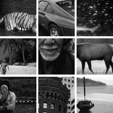
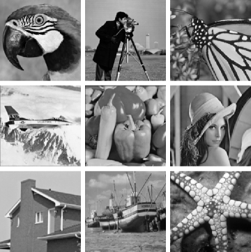
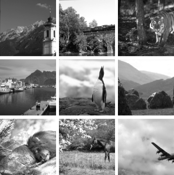
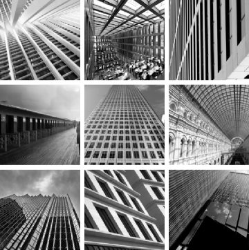
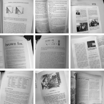
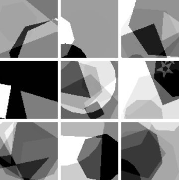
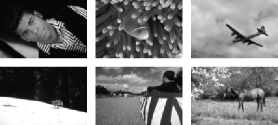
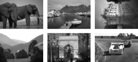
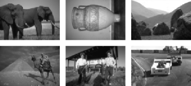
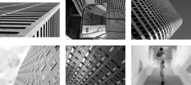
We perform controlled experiments on datasets with different signal and noise structure to evaluate the broad applicability of GainTuning (see Figure 6 for a visual summary of datasets). We describe each dataset below:
Generic natural images. We use 400 images from BSD400 [34] dataset for pre-training CNNs. We evaluate two test sets, Set12 and Set68, with 12 and 68 images for testing [65].
Images of urban scenes. We evaluate generalization capabilities of GainTuning using a dataset of images captured in urban settings, Urban100 [22]. These images often contain repeating patterns and structures, unlike generic natural images (see Figure 6). We evaluate GainTuning on the first 50 images from this dataset.
Images of scanned documents. We use images of scanned documents from the IUPR dataset [4]. The original images are very high resolution, and one of our baseline methods, Self2Self [46], requires long computational time (>24 hours per image) for such high resolution images. Therefore, we resized the images in IUPR dataset by a factor of 6. We used the first 50 images from the dataset for evaluation.
Simulated piecewise constant images. We use a dataset of simulated piecewise constant images. These images have constant regions with boundaries consisting of various shapes such as circles and lines with different orientations. The constant region has an intensity value sampled from a uniform distribution between and (see Figure 6). Piecewise constant images provide a crude model for natural images [35, 44, 31]. We use GainTuning to adapt a CNN trained on this dataset to generic natural images (Set12). This experiment demonstrates the ability of GainTuning to adapt from a simple simulated dataset to a significantly more complex real dataset.
| BSD400 | Set12 |
 |
 |
| BSD68 | Urban100 |
 |
 |
| IUPR | Piecewise constant images |
 |
 |
Simulated transmission electron microscopy data. The TEM image data used in this work correspond to images from a widely utilized catalytic system, which consist of platinum (Pt) nanoparticles supported on a larger cerium (IV) oxide (CeO2) nanoparticle. We use the simulated TEM image dataset introduced in Ref. [38] for pre-training CNNs. The simulated dataset contains 1024 x 1024 images, which are binned to match the approximate pixel size of the experimentally acquired real image series (described below). To equate the intensity range of the simulated images with those acquired experimentally, the intensities of the simulated images were scaled by a factor which equalized the vacuum intensity in a single simulation to the average intensity measured over a large area of the vacuum in a single 0.025 second experimental frame (i.e., 0.45 counts per pixel in the vacuum region). Furthermore, during TEM imaging multiple electron-optical and specimen parameters can give rise to complex, non-linear modulations of the image contrast. These parameters include the objective lens defocus, the specimen thickness, the orientation of the specimen, and its crystallographic shape/structure. Various combinations of these parameters may cause the contrast of atomic columns in the image to appear as black, white, or an intermediate mixture of the two. To account for this, the simulated dataset contains various instances of defocus, tilt, thickness, and shape/structure. We refer interested readers to Ref. [38] for more details.
Real transmission electron microscopy data. The real data consist of a series of images of the Pt/CeO2 catalyst. The images were acquired in a N2 gas atmosphere using an aberration-corrected FEI Titan transmission electron microscope (TEM), operated at 300 kV and coupled with a Gatan K2 IS direct electron detector [38]. The detector was operated in electron counting mode with a time resolution of 0.025 sec/frame and an incident electron dose rate of 5,000 e-/Å2/s. The electromagnetic lens system of the microscope was tuned to achieve a highly coherent parallel beam configuration with minimal low-order aberrations (e.g., astigmatism, coma), and a third-order spherical aberration coefficient of approximately -13 m. We refer interested readers to Ref. [38] for more details.
Appendix C Details of pre-training and GainTuning
In this section, we describe the implementation details of the pre-training process and our proposed GainTuning framework.
C.1 Overview
While performing GainTuning, we include a scalar multiplier parameter (gain) in every channel of the convolutional layers in the denoising CNN. We do not optimize the gain for the last layer of the network. We describe the general optimization process for GainTuning here, and describe any additional modifications for specific datasets in the respective subsections.
Data. We perform GainTuning on patches extracted from the noisy image. We extracted patches for the electron microscopy dataset, and patches for all other datasets. We do not perform any data augmentation on the extracted patches.
BatchNorm layers during GainTuning. If the denoising CNN contains batch normalization (BN) layers (only DnCNN [65] and BFCNN [37] in our experiments), we freeze these parameters during GainTuning. That is, we do not re-estimate the mean and standard deviation parameter for each layer from the test data. Instead, we re-use the original values estimated from pre-training dataset, and re-purposed the learnable parameter in the batch norm layer as the Gain parameter.
Optimization. We train with Adam [26] optimizer for 100 steps with a starting learning rate of which was reduced to after the step. Here, we define each step as a pass through random patches extracted from the test image. When performing experiments to compare optimizing all parameters vs optimizing only gain during the adaptation process, we kept the learning rate constant at for both options, and trained for 1000 steps.
C.2 Natural images
Pre-training dataset. Our experiments are carried out on natural images from the Berkeley Segmentation Dataset [34]. We use a training set of images. The training set is augmented via downsampling, random flips, and random rotations of patches in these images [65]. We train the CNNs on patches of size , which yields a total of 541,600 clean training patches.
Pre-training process. We train DnCNN, BFCNN and UNet using the Adam Optimizer [26] for epochs with an initial learning rate of and a decay factor of for every 10 epochs after the , with no early stopping [37].
GainTuning. We follow the same procedure as Section C.1.
C.3 Piecewise constant images
Pre-training dataset. We generated a synthetic dataset of piecewise constant images with the varied boundary shapes like slanted lines and circles (see Figure 6). The intensity values of the constant regions were uniformly sampled between and . The generated patches were of size to mimic the training process for natural images [65].
Pre-training. We train DnCNN, BFCNN and UNet using the Adam Optimizer [26] using the same process as in Section C.2. For each epoch, we generated random patches.
GainTuning . We used Adam [26] with a starting learning rate of reduced to after 20 steps for adapting CNNs trained on piecewise constant function to natural images. We trained for 100 steps in total.
C.4 Electron microscope data
Pre-training dataset. Our experiments are carried out on patches extracted from about simulated TEM introduced in Ref. [38]. The training set is augmented via downsampling, random flips, and random rotations of patches in these images [38, 59].
Optimization Details: We trained using Adam [26] optimizer with a starting learning of . The learning rate was decreased by a factor of at checkpoints during a total training of epochs [38].
GainTuning. We performed GainTuning using Adam [26] optimizer with a constant learning rate of for 100 steps. Each step consisted of 1000 randomly sampled patches of size extracted from the test image.
C.5 Computational resources used
The computations were performed on an internal cluster equipped with NVIDIA RTX8000 and NVIDIA V100 GPUs. We used open-source pre-trained networks when available.
Appendix D Approximation for SURE
Let be an -dimensional ground-truth random vector and let be a corresponding noisy observation, where . Stein’s Unbiased Risk Estimator (SURE) provides an expression for the mean-squared error between and the denoised estimate (where denotes an arbitrary denoising function), which only depends on the distribution of noisy observations :
| (8) |
The last term in the equation, called divergence, is costly to compute. Therefore, we use a Monte Carlo approximation of SURE introduced by Ref. [47] in our implementation. The approximation is given by:
| (9) |
Appendix E GainTuning prevents overfitting
We perform controlled experiments to compare test-time updating of (1) all parameters of a CNN, and (2) only the gain parameters. We briefly describe each experiment and our findings in this section.
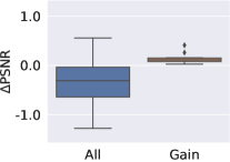
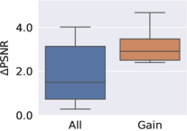
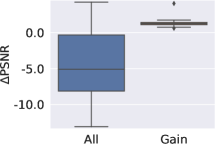
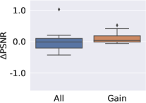
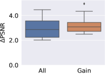
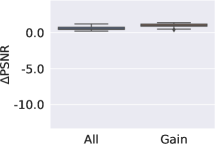
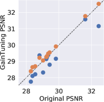
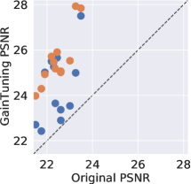
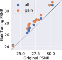
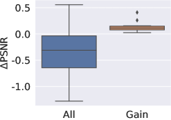
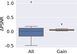
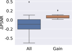
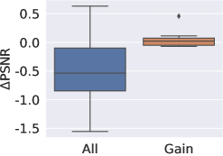
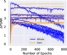
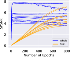
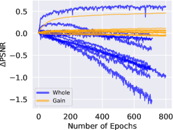
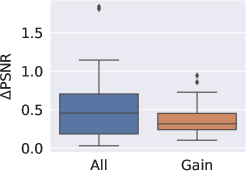
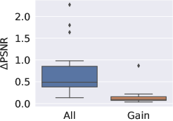
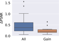
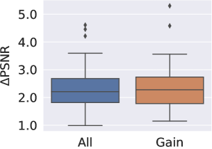
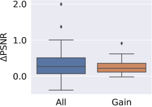
Comparison across different cost functions. We fine-tune (a) all parameters, and (b) only gain parameters of a DnCNN [65] model when the test image is (1) in-distribution, (2) corrupted with out-of-distribution noise and (c) contains image features which are different from the training set. Fine-tuning only the gain parameters outperforms fine-tuning all parameters in all of these situations for different choices of cost functions (see Figure 7 for summary statistics as a box plot and Figure 8 for improvements on individual data points visualized as a scatter plot)
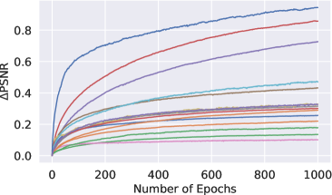
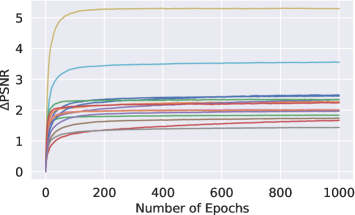
Comparison across different architectures. We fine-tune (a) all parameters, and (b) only gain parameters of a DnCNN [65], BFCNN [37] and, UNet [49] model when the test image is (a) in-distribution, (b) corrupted with out-of-distribution noise and (c) contains image features which are different from the training set. Fine-tuning only the gain parameters often outperforms fine-tuning all parameters in all of these situations for different choices of cost functions (see Figure 9). Figure 9 shows results for a CNN trained on generic natural images and tested on images of urban scenes. In this case, training all parameters of the CNN outperforms training only the gains (see Section 7 for a discussion). Interestingly, training gains is comparable to training all parameters when we corrupt the images from urban scenes with a noise level that is also outside the training range (see Figure 10).
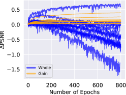
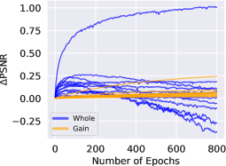
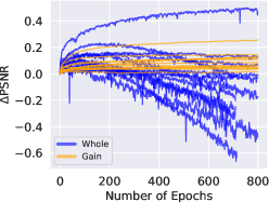
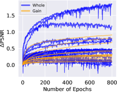
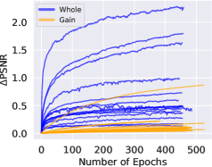
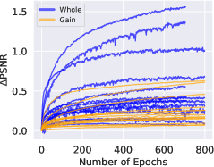
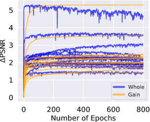
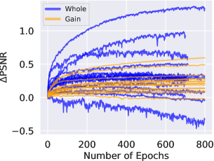
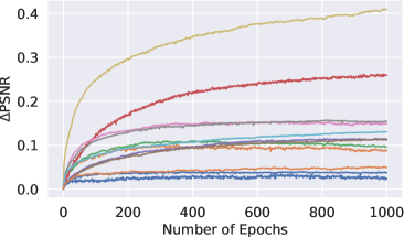
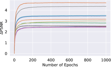
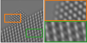
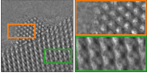
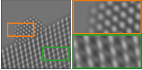
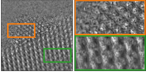
GainTuning does not require early stopping. Optimizing all parameters of a CNN during adaptation often results in overfitting (see Figure 9). In contrast, optimizing only the gain parameters for longer periods of time results improves performance without overfitting (Figure11).
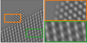
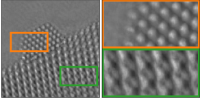
Real electron microscopy data. We fine-tune (a) all parameters, and (b) gain parameters to adapt a CNN to real images of nanoparticle acquired through an electron microscope. The CNN was pre-trained on the simulated data described in Section B. Optimizing only the gain parameters outperforms optimizing all parameter and does not require early stopping (Figure 12)
| Loss | In-distribution | Out-of-distribution noise | Out-of-distribution signal |
| SURE |
|
|
|
| Noise Resampling |
|
|
|
| Loss | In-distribution | Out-of-distribution noise | Out-of-distribution signal |
| SURE |
|
|
|
| Noise Resampling |
|
|
|
| In distribution. Natural images () Set12 () | ||
 |
 |
 |
 |
 |
 |
| Out-of-distribution noise. Natural images () Set12 () | ||
 |
 |
 |
 |
 |
 |
| Out-of-distribution signal. Natural images () Urban100 () | ||
 |
 |
 |
 |
 |
 |
| DnCNN | UNet | BFCNN |
| DnCNN | BFCNN |
|
 |
|
 |
| In-distribution Natural images () Set12 | Out-of-distribution noise Natural images () Set12 |
|---|---|
 |
 |
| Out-of-distribution image Natural images () Urban100 | Out-of-distribution image and noise Natural images () Urban100 |
 |
 |
| Gradient Steps | All parameters | Gain parameters |
| 0 |
|

|
| 1.5K |
|
|
| 2.5K |
|
|
| 5K |
|

|
| 10K |
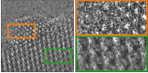
|

|
| 25K |

|
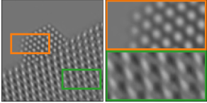
|
| 50K |
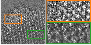
|
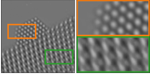
|
Appendix F Performance of GainTuning
F.1 In-distribution test image
Different architectures. We evaluated DnCNN, UNet and BFCNN architectures for this task. All models were trained on denoising Gaussian white noise of standard deviation from generic natural images. Results of DnCNN and UNet are presented in Figure 3 in the main paper. Results for the BFCNN architecture are provided in Table 2.
Different cost functions. We provide the results of evaluating DnCNN architecture with different cost functions in Table 5.
Distribution of improvements. We visualize the distribution of improvements in denoising performance for different architectures after performing GainTuning using the SURE cost function in Figure 13. As discussed in Section 7, if the CNN is optimized well and the test image is in-distribution, GainTuning can degrade performance. This degradation is atypical (3 out of 408 total evaluations) and very small (maximum degradation of 0.02 dB in PSNR).
| Model | Set12 | Set68 | |||
| Pre-trained | GainTuning | Pre-trained | GainTuning | ||
| BFCNN | 29.52 | 29.61 | 28.36 | 28.45 | |
| DnCNN | UNet | ||||||||||||
| 30 | 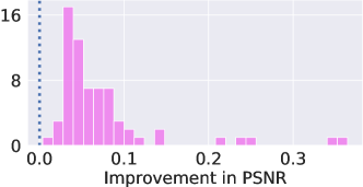 |
 |
|||||||||||
|
|
||||||||||||
| 40 | 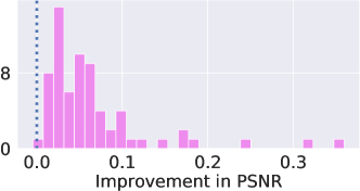 |
 |
|||||||||||
|
|
||||||||||||
| 50 | 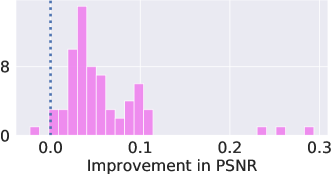 |
 |
|||||||||||
|
|
F.2 Out-of-distribution noise
| Test set | Trained on | Baselines | ||||||
| Bias Free Model [37] | Trained on | LIDIA [58] | S2S [46] | |||||
|---|---|---|---|---|---|---|---|---|
| Pre-trained | GainTuning | Pre-trained | Adapted | |||||
| Set12 | 22.45 | 25.54 | 25.59 | 25.50 | 23.69 | 25.01 | 24.61 | |
| 18.48 | 24.57 | 24.94 | 24.88 | 22.12 | 24.17 | 23.64 | ||
| BSD68 | 22.15 | 24.89 | 24.87 | 24.88 | 23.28 | 24.57 | 24.29 | |
| 18.72 | 24.14 | 24.38 | 24.36 | 21.87 | 23.97 | 23.65 | ||
Different Architectures. We summarize the results using DnCNN in Table 4 in the main paper. Figure 9 shows that the UNet architecture is also able to generalize to out-of-distribution noise.
Different Loss Functions. We provide the results of evaluating DnCNN architecture with different cost functions in Table 5.
Comparison to baselines. Table 3 summarizes the result of evaluating a DnCNN trained on generic natural images for on a test set of generic natural images corrupted with , which is outside the training range of the network. GainTuning is able to generalize effectively to this out-of-distribution test set. GainTuning achieves comparable performance to a network trained with supervision on a large range of noise levels (), and a bias-free model which is explicitly designed to generalize to noise levels outside the training range. GainTuning also outperforms LIDIA [58] (a specialized architecture and adaptation procedure). and Self2Self [46] (a method trained exclusively on the test image).
F.3 Out-of-distribution image
| Training Data | Test Data | DnCNN [65] | Baselines | ||||
|---|---|---|---|---|---|---|---|
| LIDIA [58] | S2S [46] | ||||||
| Pre-trained | GainTuning | Pre-trained | Adapted | ||||
| (a) | Piecewise constant | Natural images | 27.31 | 28.60 | - | - | 29.21 |
| (b) | Natural images | Urban images | 28.35 | 28.79 | 28.54 | 28.71 | 29.08 |
| (c) | Natural images | Scanned documents | 30.02 | 30.73 | 30.05 | 30.23 | 30.86 |
Different Architectures. We summarize the results using DnCNN in Table 4 in the main paper. Figures 9 show that the UNet and BFCNN architectures are also able to generalize to test data with different characteristics from the training data when adapted using GainTuning .
Different Loss Functions. We provide the results of evaluating the DnCNN architecture with different cost functions in Table 5.
Comparison to baselines. Results of comparison to LIDIA [58], a specialized architecture to perform adaptation, and Self2Self [46] a method trained exclusively on the test image is summarized in Table 4. While GainTuning outperforms LIDIA, it does not match the performance of Self2Self (see Section 7 for a discussion on this).
F.4 Out-of-distribution noise and image
We evaluated the ability of GainTuning to adapt to test images which have different characteristics from those in the training set, and are additionally corrupted with a noise distribution that is different from the noise in the training set. Figure 10 shows that GainTuning is successful in this setting. The CNN was pre-trained on natural images corrupted with Gaussian white noise of standard deviation . We used GainTuning to adapt this CNN to a test set of images taken in urban setting (see Section B for a discussion on how it is different from natural images), corrupted with Gaussian noise of standard deviation (which is outside the training range of ).
F.5 Application to Electron Microscopy
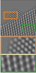
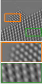
| (a) Noisy image | (b) Unsupervised training only on (a) [46] | (c) Supervised training on simulated data [38] | (d) GainTuning on CNN trained on sim. data (c) | (e) Estimated reference image |
|---|---|---|---|---|
 |
 |
 |
 |
 |
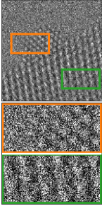
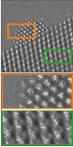
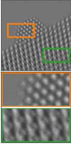
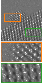
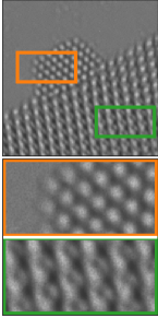
| Noisy image | Blind-spot [29] | Blind-spot Early Stopping [51] | UDVD [51] | UDVD Early stopping [51] |
|---|---|---|---|---|
 |
 |
 |
 |
 |
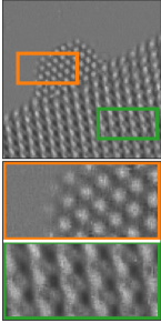
| Self2Self [46] | Pre-trained [38, 59] | GainTuning Noise resampling | GainTuning blind-spot | Estimated reference |
 |
 |
 |
 |
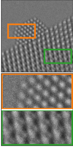 |
Comparison to pre-trained CNN. As discussed in Section 5.4, a CNN [29] pre-trained on the simulated data fails to reconstruct the pattern of atoms faithfully. We show an additional example (Figure 14) to support this. GainTuning applied to the pre-trained CNN using the blind-spot loss correctly recovers this pattern (green box in Figure 14 (d), (e)) reconstructing the small oxygen atoms in the CeO2 support. GainTuning with noise resampling failed to reproduce the support pattern, probably because it is absent from the initial denoised estimate (see Figure 15).
Comparison to baselines. Since no ground-truth images are available for this dataset (see Section 5.4), we average 40 different acquisitions of the same underlying image to obtain an estimated reference for visual reference. We also compare GainTuning to state-of-the-art dataset based unsupervised methods, which are trained on these 40 images.
-
•
Blind-spot net [29] is a CNN which is constrained to predict the intensity of a pixel as a function of the noisy pixels in its neighbourhood, without using the pixel itself. This method is competitive with the current supervised state-of-the-art CNN on photographic images. However, when applied to this dataset it produces denoised images with visible artefacts (see Figure 15). Ref. [51] shows that this may be because of the limited amount of data ( noisy images): They trained a blind-spot net on simulated training sets of different sizes, observing that the performance on held-out data is indeed poor when the training set is small, but improves to the level of supervised approaches for large training sets.
-
•
Unsupervised Deep Video Denoising (UDVD) [51] is an unsupervised method for denoising video data based on the blind-spot approach. It estimates a denoised frame using consecutive noisy frames around it. Our real data consists of frames acquired sequentially. UDVD produces better results than blind-spot net, but still contains visible artefacts, including missing atoms (see Figure 15). Note that UDVD uses noisy images as input, and thus has more context to perform denoising than the other methods (including GainTuning ).
-
•
Blind-spot net with early stopping. In Ref. [51] it is shown that early stopping based on noisy held-out data can boost the performance of blind-spot nets. Here we used images for training the blind-spot net and the remaining images as a held-out validation set. We chose the model parameters that minimized the mean squared error between the noisy validation images and the corresponding denoised estimates. The results (shown in Figure 15) are significantly better than those of the standard blind-spot network. However, there are still noticeable artefacts, which include missing atoms. This method is similar in spirit to GainTuning - but uses a different strategy to prevent overfitting.
- •
F.6 Different loss functions
GainTuning can be used in conjunction with any unsupervised denoising cost function. We explore three different choices - SURE, noise resampling, and blind-spot cost functions (see Section 4), and summarize our finding in Table 5.
SURE loss outperforms other choices in most experiments. Noise resampling has comparable performance to SURE when the test data is in-distribution, or when it is corrupted with out-of-distribution noise. However, noise resampling generally under-performs SURE when the test images have different features from the training images. A possible explanation for this is that noise resampling relies on the initial denoised image to fine-tune and, therefore, it may not be able to exploit features which are not present in the initial estimate. In contrast, the SURE cost function is computed on the noisy test image itself, thereby enabling it to adapt to features that the pre-trained network may be agnostic to.
Finally, adapting using blind-spot cost function often under-performs both SURE and noise resampling. The difference in performance is reduced at higher noise levels (see also Section 5.4 where we use blind-spot cost function for experiments with real TEM data with very high noise). The reason for this could be that at higher noise levels, the information contained in a single pixel becomes less relevant for computing the corresponding denoised estimate (in fact, the regularization penalty on “self pixel‘ for SURE cost function (Section 4) increases as the noise level increases). Therefore, the loss of performance incurred by the blind-spot cost function is diminished. At lower noise levels (particularly when the images are in-distribution), adapting using blind-spot cost function will force the pre-trained network to give up using the “self pixel“, which results in a degraded performance. An alternative to adapting a generic pre-trained network using blind-spot architecture is to use a CNN that is architecturally constrained to include a blind-spot. In Table 6, we show that adapting such a CNN using blind-spot loss improves the performance its performance. However, the overall performance of this architecture is in general lower than the networks which also use the “self pixel“. We refer interested readers to Ref. [29, 28, 61] for approaches to incorporate the noisy pixel into the denoised estimate.
| GainTuning with | |||||
| Pre-training | SURE | Noise resampling | Blind-spot (Noise2Self [3]) | ||
|---|---|---|---|---|---|
| in distribution | Set12 | 29.52 | 29.62 | 29.63 | 29.50 |
| BSD68 | 28.39 | 28.46 | 28.40 | 28.36 | |
| out-of-distribution noise | Set12 | 18.48 | 24.57 | 24.11 | 22.93 |
| BSD68 | 18.72 | 24.14 | 23.65 | 22.50 | |
| out-of-distribution image | Piecewise constant Natural images | 27.31 | 28.60 | 28.29 | 27.39 |
| Natural images Urban100 | 28.35 | 28.79 | 28.79 | 28.29 | |
| Natural images Scanned documents | 30.02 | 30.73 | 30.57 | 29.23 | |
| in-distribution | out-of-distribution image | |||
| Set12 | BSD68 | Urban100 (urban scenes) | IUPR (scanned documents) | |
|---|---|---|---|---|
| Pre-trained | 27.92 | 26.47 | 26.59 | 28.25 |
| GainTuning | 27.92 | 26.61 | 26.85 | 28.40 |
Appendix G Analysis
G.1 What kind of images benefit the most from adaptive denoising?
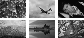
We sort images by the improvement in performance (PSNR) achieved with GainTuning. We observe that the ordering of images is similar for different models and cost functions (See Figure 16), implying that the improvement in performance is mostly dependent on the image content. The images with largest improvement typically contain repeated patterns and are more structured. Repetition of patterns effectively provides multiple samples from which the unsupervised refinement can benefit.
| DnCNN | UNet | ||
| In-distribution | Top 6 |
|
|
| Bottom 6 |
|
|
|
| Out-of-distribution image | Top 6 |
|
|
| Bottom 6 |
|
|
G.2 Generalization via GainTuning
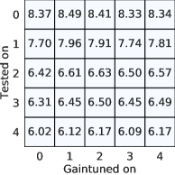
| (a) Dataset of scanned documents | (b) Natural images with out-of-distribution noise | (c) Equivalent bias before and after gaintuning |
|---|---|---|
 |
 |
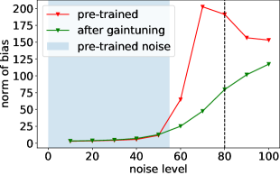 |
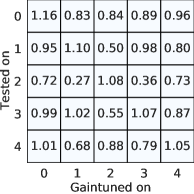
We investigate the generalization capability of GainTuning. We observe that a CNN adapted to a particular image via GainTuning generalizes effectively to other similar images. Figure 17 shows that GainTuning can achieve generalization to images that are similar to the test image used for adaptation on two examples: (1) adapting a network to an image of a scanned document generalizes to other scanned documents, and (2) adapting a a network to an image with out-of-distribution noise generalizes to other images with similar noise statistics.
G.3 How does GainTuning adapt to out-of-distribution noise?
Let be a noisy image processed by a CNN. Using the first-order Taylor approximation, the function computed by a denoising CNN may be expressed as an affine function
| (10) |
where is the Jacobian of evaluated at input , and represents the net bias. In [37], it was shown that the bias tends to be small for CNNs trained to denoise natural images corrupted by additive Gaussian noise, but is a primary cause of failures to generalize to noise levels not encountered during training. Figure 17 shows that GainTuning reduces the net bias of CNN, facilitating the generalization to new noise levels.
G.4 How does GainTuning adapt to out-of-distribution images?
In order to understand how GainTuning adapt to out-of-distribution images, we examine the adaptation of a CNN pre-trained on piecewise constant to natural images. Piecewise constant images have large areas with constant intensities, therefore, CNNs trained on these images tends to average over large areas. This is true even when the test image contains detailed structures. We verify this by forming the affine approximation of the network (eq. 10) and visualizing the equivalent linear filter [37], as explained below:
Let be a noisy image processed by a CNN. We process the test image using a Bias-Free CNN [37] so that the net bias is zero in its first-order Taylor decomposition (10). When , (10) implies that the th pixel of the output image is computed as an inner product between the th row of , denoted , and the input image:
| (11) |
The vectors can be interpreted as adaptive filters that produce an estimate of the denoised pixel via a weighted average of noisy pixels. As shown in Figure 5 the denoised output of CNN pre-trained on piece wise constant images is over-smoothed and the filters average over larger areas. After GainTuning the model learns to preserve the fine features much better, which is reflected in the equivalent filters
