Theoretical Study and Comparison of SPSA and RDSA Algorithms with Different Perturbations

Yiwen Chen
Abstract

Stochastic approximation (SA) algorithms are widely used in system optimization problems when only noisy measurements of the system are available. This paper studies two types of SA algorithms in a multivariate Kiefer-Wolfowitz setting: random-direction SA (RDSA) and simultaneous-perturbation SA (SPSA), and then describes the bias term, convergence, and asymptotic normality of RDSA algorithms. The gradient estimations in RDSA and SPSA have different forms and, consequently, use different types of random perturbations. This paper looks at various valid distributions for perturbations in RDSA and SPSA and then compares the two algorithms using mean-square errors computed from asymptotic distribution. From both a theoretical and numerical point of view, we find that SPSA generally outperforms RDSA.

††1. A compressed version of this paper appears in the 2021 55rd Annual Conference on Information Sciences and Systems (CISS), Mar 2021.
2. Contact Information: ychen385@jh.edu / yyiwen1207@gmail.com

1 Introduction

Stochastic approximation is a well-known recursive procedure for finding roots of equations in the presence of noisy measurements. Consider a smooth p𝑝p-dimensional loss function L:ℝp→ℝ:𝐿→superscriptℝ𝑝ℝL:\,\mathbb{R}^{p}\rightarrow\mathbb{R}, with gradient π’ˆ:ℝp→ℝp:π’ˆβ†’superscriptℝ𝑝superscriptℝ𝑝\bm{g}:\mathbb{R}^{p}\rightarrow\mathbb{R}^{p}. Assume that L𝐿L has a unique minimum π›‰βˆ—βˆˆβ„psuperscript𝛉superscriptℝ𝑝\bm{\uptheta}^{*}\in\mathbb{R}^{p}; i.e. L​(π›‰βˆ—)≀L​(𝛉)𝐿superscript𝛉𝐿𝛉L(\bm{\uptheta}^{*})\leq L(\bm{\uptheta}) for all π›‰βˆ—βˆˆβ„psuperscript𝛉superscriptℝ𝑝\bm{\uptheta}^{*}\in\mathbb{R}^{p}, and π’ˆβ€‹(π›‰βˆ—)=πŸŽπ’ˆsuperscript𝛉0\bm{g}(\bm{\uptheta}^{*})=\bm{0}. In many cases where only noisy measurements of the gradient are available, the Robbins-Monro stochastic approximation (SA) algorithm is widely used with the form of:

𝛉^k+1=𝛉^kβˆ’ak​𝒀k​(𝛉^k).k=0,1,2,…formulae-sequencesubscriptbold-^π›‰π‘˜1subscriptbold-^π›‰π‘˜subscriptπ‘Žπ‘˜subscriptπ’€π‘˜subscriptbold-^π›‰π‘˜π‘˜012…\displaystyle\bm{\hat{\uptheta}}_{k+1}=\bm{\hat{\uptheta}}_{k}-a_{k}\bm{Y}_{k}(\bm{\hat{\uptheta}}_{k}).\;k=0,1,2,... (1)

where 𝒀k​(𝛉^k)=βˆ‚Q/βˆ‚π›‰subscriptπ’€π‘˜subscriptbold-^π›‰π‘˜π‘„π›‰\bm{Y}_{k}(\bm{\hat{\uptheta}}_{k})=\partial{Q}/\partial{\bm{\uptheta}} represents a direct noisy measurement of the true gradient π’ˆk​(𝛉^k)subscriptπ’ˆπ‘˜subscriptbold-^π›‰π‘˜\bm{g}_{k}(\bm{\hat{\uptheta}}_{k}) for Q𝑄Q in the representation L​(𝛉)=E​[Q​(𝛉,𝑽)]𝐿𝛉𝐸delimited-[]𝑄𝛉𝑽L(\bm{\uptheta})=E[Q(\bm{\uptheta,V})] with 𝑽𝑽\bm{V} corresponding to the randomness in the problem. ak>0subscriptπ‘Žπ‘˜0a_{k}>0 is the step size, determining the convergence of the algorithm.

However, in most practical cases, such direct measurement is difficult to obtain and only noisy measurements of the loss function are available. Then it comes to the use of gradient-free algorithms. There are several common algorithms such as the finite-difference (FD) SA, random-direction SA (RDSA) and the simultaneous-perturbation SA (SPSA). All of them use the measurement of the loss function to estimate the gradient. The FDSA algorithm has also been discussed comprehensively in [15]. It has an i𝑖ith component in the form of:

π’ˆ^k​i​(𝛉^k)=y​(𝛉^k+ck​𝒆i)βˆ’y​(𝛉^kβˆ’ck​𝒆i)2​ck,subscript^π’ˆπ‘˜π‘–subscript^π›‰π‘˜π‘¦subscript^π›‰π‘˜subscriptπ‘π‘˜subscript𝒆𝑖𝑦subscript^π›‰π‘˜subscriptπ‘π‘˜subscript𝒆𝑖2subscriptπ‘π‘˜\displaystyle\hat{\bm{g}}_{ki}(\hat{\bm{\uptheta}}_{k})=\dfrac{y(\hat{\bm{\uptheta}}_{k}+c_{k}\bm{e}_{i})-y(\hat{\bm{\uptheta}}_{k}-c_{k}\bm{e}_{i})}{2c_{k}}, (2)

where 𝒆isubscript𝒆𝑖\bm{e}_{i} denotes the unit vector along the i𝑖ith axis and y𝑦y is the noisy measurement of the loss value and ck>0subscriptπ‘π‘˜0c_{k}>0 defines the difference magnitude. The pair {ak,ck}subscriptπ‘Žπ‘˜subscriptπ‘π‘˜{\{a_{k},c_{k}}\} represents the gain sequences. Nevertheless, the FDSA algorithm shows inefficiency in solving problems with high dimension due to its use of 2​p2𝑝2p measurements of L𝐿L per iteration. The other two RDSA and SPSA approaches, alleviate this problem by requiring only two system simulations regardless of the parameter dimension.

Several papers have discussed the three SA algorithms. Spall has discussed details of FDSA and SPSA algorithms in [13] and [15]; Kushner discussed the RDSA algorithm in [9]; Blakney and Zhu compared FDSA and SPSA algorithms in [2] and Chin compared the three algorithms using mean-square errors in [3]. Because the FDSA and SPSA algorithms have been well analyzed, this paper will mainly focus on the RDSA algorithm. Some papers investigated the theoretical foundation for RDSA algorithms such as [1], [18] and [3]; however, some of them gave the illustration only briefly. This paper is going to arrange and organize those different versions of theoretical proofs to show the convergence and asymptotic normality. After that, we will conduct the comparison between RDSA and SPSA using Mean-Square Error and present certain conditions under which SPSA outperforms RDSA with specific perturbations.

The remainder of this paper is organized as follows. Section 2 introduces the general formulation of the SPSA and RDSA algorithms. Section 3 covers the bias term, convergence condition, and asymptotic normality of RDSA algorithm and leads to the comparison of relative accuracy of SPSA and RDSA. Section 4 presents several numerical studies to assist the theoretical conclusion in Section 3. Especially, this paper uses the skewed-quartic function as an example to show how the theory works on the performance of distinct distributed perturbation in SPSA and RDSA.

2 Background

This section briefly discusses the SPSA algorithm and the RDSA algorithm with their estimates for the gradient, π’ˆ^​(𝛉^k)^π’ˆsubscript^π›‰π‘˜\hat{\bm{g}}(\hat{\bm{\uptheta}}_{k}).

SPSA (β€˜Simultaneous Perturbation Stochastic Algorithm’) has been well discussed in [15, Chap. 7] and [14]. The estimate for π’ˆβ€‹(𝛉^k)π’ˆsubscript^π›‰π‘˜\bm{g}(\hat{\bm{\uptheta}}_{k}) is in the form of:

π’ˆ^k​(𝛉^k)=y​(𝛉^k+ckβ€‹πš«k)βˆ’y​(𝛉^kβˆ’ckβ€‹πš«k)2​ckβ€‹πš«k,subscript^π’ˆπ‘˜subscript^π›‰π‘˜π‘¦subscript^π›‰π‘˜subscriptπ‘π‘˜subscriptπš«π‘˜π‘¦subscript^π›‰π‘˜subscriptπ‘π‘˜subscriptπš«π‘˜2subscriptπ‘π‘˜subscriptπš«π‘˜\displaystyle\hat{\bm{g}}_{k}(\hat{\bm{\uptheta}}_{k})=\dfrac{y(\hat{\bm{\uptheta}}_{k}+c_{k}\bm{\Delta}_{k})-y(\hat{\bm{\uptheta}}_{k}-c_{k}\bm{\Delta}_{k})}{2c_{k}\bm{\Delta}_{k}},

where y​(𝛉^kΒ±ckβ€‹πš«k)=L​(𝛉^kΒ±ckβ€‹πš«k)+Ο΅k(Β±)𝑦plus-or-minussubscript^π›‰π‘˜subscriptπ‘π‘˜subscriptπš«π‘˜πΏplus-or-minussubscript^π›‰π‘˜subscriptπ‘π‘˜subscriptπš«π‘˜subscriptsuperscriptΟ΅plus-or-minusπ‘˜y(\hat{\bm{\uptheta}}_{k}\pm c_{k}\bm{\Delta}_{k})=L(\hat{\bm{\uptheta}}_{k}\pm c_{k}\bm{\Delta}_{k})+\upepsilon^{(\pm)}_{k} with Ο΅k(Β±)subscriptsuperscriptΟ΅plus-or-minusπ‘˜\upepsilon^{(\pm)}_{k} representing measurement noise term that satisfies E​[Ο΅k(+)βˆ’Ο΅k(βˆ’)]=0𝐸delimited-[]subscriptsuperscriptΟ΅π‘˜subscriptsuperscriptΟ΅π‘˜0E[\upepsilon^{(+)}_{k}-\upepsilon^{(-)}_{k}]=0. 𝚫kβˆˆβ„psubscriptπš«π‘˜superscriptℝ𝑝\bm{\Delta}_{k}\in\mathbb{R}^{p} is a vector of p𝑝p mutually independent mean-zero random variables representing the perturbation, which satisfies certain conditions, and 𝚫kβˆ’1subscriptsuperscript𝚫1π‘˜\bm{\Delta}^{-1}_{k} represents the vector of inverse components. There’s no specific type of distribution for 𝚫ksubscriptπš«π‘˜\bm{\Delta}_{k} as long as the perturbation satisfies general conditions mentioned in [15, Chap. 7] (Principally, mean 0, symmetric, finite moments and certain inverse moments). Usually, 𝚫ksubscriptπš«π‘˜\bm{\Delta}_{k} can be chosen as Bernoulli, U-shape, and other distributions. The range of choices is restricted due to the main constraint that the inverse moment E​(|1/Ξ”k​m|)𝐸1subscriptΞ”π‘˜π‘šE(|1/\Delta_{km}|) should be finite. Many common distributions, such as Gaussian distribution and Uniform distribution, cannot be applied to the SPSA algorithm since they contain too much probability mass near 0.

For RDSA (β€˜Random Direction Stochastic Algorithm’), the estimate for π’ˆβ€‹(𝛉^k)π’ˆsubscript^π›‰π‘˜\bm{g}(\hat{\bm{\uptheta}}_{k}) is in the form of:

π’ˆ^k​(𝛉^k)=y​(𝛉^k+ck​𝝅k)βˆ’y​(𝛉^kβˆ’ck​𝝅k)2​ck​𝝅k,subscript^π’ˆπ‘˜subscript^π›‰π‘˜π‘¦subscript^π›‰π‘˜subscriptπ‘π‘˜subscriptπ…π‘˜π‘¦subscript^π›‰π‘˜subscriptπ‘π‘˜subscriptπ…π‘˜2subscriptπ‘π‘˜subscriptπ…π‘˜\displaystyle\hat{\bm{g}}_{k}(\hat{\bm{\uptheta}}_{k})=\dfrac{y(\hat{\bm{\uptheta}}_{k}+c_{k}\bm{\pi}_{k})-y(\hat{\bm{\uptheta}}_{k}-c_{k}\bm{\pi}_{k})}{2c_{k}}\bm{\pi}_{k},

where 𝝅kβˆˆβ„psubscriptπ…π‘˜superscriptℝ𝑝\bm{\pi}_{k}\in\mathbb{R}^{p} is a vector of Monte-Carlo generated random variables satisfying certain regularity conditions and normalized so that ‖𝝅kβ€–2=psuperscriptnormsubscriptπ…π‘˜2𝑝||\bm{\pi}_{k}||^{2}=p . Unlike SPSA, the requirement for finite inverse moment is released for 𝝅ksubscriptπ…π‘˜\bm{\pi}_{k} in RDSA, so the range of choices of distribution for 𝝅ksubscriptπ…π‘˜\bm{\pi}_{k} is different from that for 𝚫ksubscriptπš«π‘˜\bm{\Delta}_{k} in SPSA. Several valid choices have been discussed in [18] such as axis distribution, Gaussian distribution, and Uniformly Spherical distribution where the perturbation distributes uniformly on a p𝑝p-dimensional sphere.

The main difference between the two algorithms is that in RDSA, both adjustments to 𝛉^ksubscript^π›‰π‘˜\hat{\bm{\uptheta}}_{k} and π’ˆ^k​(𝛉^k)subscript^π’ˆπ‘˜subscript^π›‰π‘˜\hat{\bm{g}}_{k}(\hat{\bm{\uptheta}}_{k}) are in the same direction 𝝅ksubscriptπ…π‘˜\bm{\pi}_{k} while the SPSA employs two different directions, 𝚫ksubscriptπš«π‘˜\bm{\Delta}_{k} and 𝛇ksubscriptπ›‡π‘˜\bm{\upzeta}_{k} with component ΞΆk​i=1/Ξ”k​isubscriptΞΆπ‘˜π‘–1subscriptΞ”π‘˜π‘–\upzeta_{ki}=1/{\Delta}_{ki}.

There are two popular choices for 𝝅ksubscriptπ…π‘˜\bm{\pi}_{k}: independent Gaussian distribution N​(0,1)𝑁01N(0,1) and Uniformly Spherical distribution with radius p𝑝\sqrt{p}. Notice that in Uniformly Spherical distribution, since there is the normalization, ‖𝝅kβ€–2=psuperscriptnormsubscriptπ…π‘˜2𝑝||\bm{\pi}_{k}||^{2}=p, variables are not independent, but uncorrelated.

3 Methodology

This section presents several results that form the theoretical basis for the RDSA algorithm, similar to those results of SPSA, which have been completely proved in [12]. The following sections consider the bias term in π’ˆ^k​(𝛉^k)subscriptbold-^π’ˆπ‘˜subscriptbold-^π›‰π‘˜\bm{\hat{g}}_{k}(\bm{\hat{\uptheta}}_{k}), the strong convergence and asymptotic normality of 𝛉^ksubscript^π›‰π‘˜\hat{\bm{\uptheta}}_{k} in the RDSA algorithm. Then we compare the performance of RDSA with SPSA using mean-square error computed with the asymptotic distribution.

3.1 The bias in π’ˆ^ksubscript^π’ˆπ‘˜\hat{\bm{g}}_{k}

The bias term in π’ˆ^ksubscript^π’ˆπ‘˜\hat{\bm{g}}_{k} is in the form of:

𝒃k​(𝛉^k)=E​[π’ˆ^k​(𝛉^k)|ΞΈ^k]βˆ’π’ˆk​(𝛉^k),subscriptπ’ƒπ‘˜subscript^π›‰π‘˜πΈdelimited-[]conditionalsubscript^π’ˆπ‘˜subscript^π›‰π‘˜subscript^πœƒπ‘˜subscriptπ’ˆπ‘˜subscriptbold-^π›‰π‘˜\displaystyle\bm{b}_{k}(\hat{\bm{\uptheta}}_{k})=E[\hat{\bm{g}}_{k}(\hat{\bm{\uptheta}}_{k})|\hat{\theta}_{k}]-\bm{g}_{k}(\bm{\hat{\uptheta}}_{k}), (3)

where Ο΅k(Β±)=y​(𝛉kΒ±ck​𝝅k)βˆ’L​(𝛉kΒ±ck​𝝅k)subscriptsuperscriptΟ΅plus-or-minusπ‘˜π‘¦plus-or-minussubscriptπ›‰π‘˜subscriptπ‘π‘˜subscriptπ…π‘˜πΏplus-or-minussubscriptπ›‰π‘˜subscriptπ‘π‘˜subscriptπ…π‘˜\upepsilon^{(\pm)}_{k}=y(\bm{\uptheta}_{k}\pm c_{k}\bm{\pi}_{k})-L(\bm{\uptheta}_{k}\pm c_{k}\bm{\pi}_{k}) is the noise on the estimate of the loss function L𝐿L, with mean 0 and variance Οƒ2superscriptΟƒ2\upsigma^{2}. Here we henceforth assume that the noise is independent with 𝛉^ksubscript^π›‰π‘˜\hat{\bm{\uptheta}}_{k} and 𝝅ksubscriptπ…π‘˜\bm{\pi}_{k}.

Calculate E​[π’ˆ^k​(𝛉^k)]𝐸delimited-[]subscript^π’ˆπ‘˜subscript^π›‰π‘˜E[\hat{\bm{g}}_{k}(\hat{\bm{\uptheta}}_{k})] and π’ˆβ€‹(𝛉^k)π’ˆsubscript^π›‰π‘˜\bm{g}(\hat{\bm{\uptheta}}_{k}) respectively:

π’ˆ^k​(𝛉^k)=subscript^π’ˆπ‘˜subscript^π›‰π‘˜absent\displaystyle\hat{\bm{g}}_{k}(\hat{\bm{\uptheta}}_{k})= y​(𝛉^k+ck​𝝅k)βˆ’y​(𝛉^kβˆ’ck​𝝅k)2​ck​𝝅k𝑦subscript^π›‰π‘˜subscriptπ‘π‘˜subscriptπ…π‘˜π‘¦subscript^π›‰π‘˜subscriptπ‘π‘˜subscriptπ…π‘˜2subscriptπ‘π‘˜subscriptπ…π‘˜\displaystyle\dfrac{y(\hat{\bm{\uptheta}}_{k}+c_{k}\bm{\pi}_{k})-y(\hat{\bm{\uptheta}}_{k}-c_{k}\bm{\pi}_{k})}{2c_{k}}\;\bm{\pi}_{k}
=L​(𝛉^k+ck​𝝅k)+Ο΅k(+)βˆ’L​(𝛉^kβˆ’ck​𝝅k)βˆ’Ο΅k(βˆ’)2​ck​𝝅kabsent𝐿subscript^π›‰π‘˜subscriptπ‘π‘˜subscriptπ…π‘˜subscriptsuperscriptΟ΅π‘˜πΏsubscript^π›‰π‘˜subscriptπ‘π‘˜subscriptπ…π‘˜subscriptsuperscriptΟ΅π‘˜2subscriptπ‘π‘˜subscriptπ…π‘˜\displaystyle=\dfrac{L(\hat{\bm{\uptheta}}_{k}+c_{k}\bm{\pi}_{k})+\upepsilon^{(+)}_{k}-L(\hat{\bm{\uptheta}}_{k}-c_{k}\bm{\pi}_{k})-\upepsilon^{(-)}_{k}}{2c_{k}}\;\bm{\pi}_{k}
=L​(𝛉^k+ck​𝝅k)βˆ’L​(𝛉^kβˆ’ck​𝝅k)2​ck​𝝅k+Ο΅k(+)βˆ’Ο΅k(βˆ’)2​ck​𝝅kabsent𝐿subscript^π›‰π‘˜subscriptπ‘π‘˜subscriptπ…π‘˜πΏsubscript^π›‰π‘˜subscriptπ‘π‘˜subscriptπ…π‘˜2subscriptπ‘π‘˜subscriptπ…π‘˜subscriptsuperscriptΟ΅π‘˜subscriptsuperscriptΟ΅π‘˜2subscriptπ‘π‘˜subscriptπ…π‘˜\displaystyle=\dfrac{L(\hat{\bm{\uptheta}}_{k}+c_{k}\bm{\pi}_{k})-L(\hat{\bm{\uptheta}}_{k}-c_{k}\bm{\pi}_{k})}{2c_{k}}\;\bm{\pi}_{k}+\dfrac{\upepsilon^{(+)}_{k}-\upepsilon^{(-)}_{k}}{2c_{k}}\bm{\pi}_{k}
=2​ckβ€‹π’ˆβ€‹(𝛉^k)T​𝝅k+16​ck3​L′′′​(𝛉¯k(+))​[𝝅kβŠ—π…kβŠ—π…k]2​ck​𝝅kabsent2subscriptπ‘π‘˜π’ˆsuperscriptsubscript^π›‰π‘˜π‘‡subscriptπ…π‘˜16subscriptsuperscript𝑐3π‘˜superscript𝐿′′′subscriptsuperscriptΒ―π›‰π‘˜delimited-[]tensor-productsubscriptπ…π‘˜subscriptπ…π‘˜subscriptπ…π‘˜2subscriptπ‘π‘˜subscriptπ…π‘˜\displaystyle=\dfrac{2c_{k}\bm{g}(\hat{\bm{\uptheta}}_{k})^{T}\bm{\pi}_{k}+\dfrac{1}{6}c^{3}_{k}L^{{}^{\prime\prime\prime}}(\bar{\bm{\uptheta}}^{(+)}_{k})[\bm{\pi}_{k}\otimes\bm{\pi}_{k}\otimes\bm{\pi}_{k}]}{2c_{k}}\;\bm{\pi}_{k}
+16​ck3​L′′′​(𝛉¯k(βˆ’))​[𝝅kβŠ—π…kβŠ—π…k]2​ck​𝝅k16subscriptsuperscript𝑐3π‘˜superscript𝐿′′′subscriptsuperscriptΒ―π›‰π‘˜delimited-[]tensor-productsubscriptπ…π‘˜subscriptπ…π‘˜subscriptπ…π‘˜2subscriptπ‘π‘˜subscriptπ…π‘˜\displaystyle+\dfrac{\dfrac{1}{6}c^{3}_{k}L^{{}^{\prime\prime\prime}}(\bar{\bm{\uptheta}}^{(-)}_{k})[\bm{\pi}_{k}\otimes\bm{\pi}_{k}\otimes\bm{\pi}_{k}]}{2c_{k}}\;\bm{\pi}_{k}
+O​(ck5)+Ο΅k(+)βˆ’Ο΅k(βˆ’)2​ck​𝝅k𝑂subscriptsuperscript𝑐5π‘˜subscriptsuperscriptΟ΅π‘˜subscriptsuperscriptΟ΅π‘˜2subscriptπ‘π‘˜subscriptπ…π‘˜\displaystyle+O(c^{5}_{k})+\dfrac{\upepsilon^{(+)}_{k}-\upepsilon^{(-)}_{k}}{2c_{k}}\bm{\pi}_{k}

where 𝛉¯k(Β±)subscriptsuperscript¯𝛉plus-or-minusπ‘˜\bar{\bm{\uptheta}}^{(\pm)}_{k} denotes points on the line segments between 𝛉^ksubscript^π›‰π‘˜\hat{\bm{\uptheta}}_{k} and 𝛉^kΒ±ck​𝝅kplus-or-minussubscript^π›‰π‘˜subscriptπ‘π‘˜subscriptπ…π‘˜\hat{\bm{\uptheta}}_{k}\pm c_{k}\bm{\pi}_{k}.

Then look at the mπ‘šmth term of π’ˆ^k​(𝛉^k)subscript^π’ˆπ‘˜subscript^π›‰π‘˜\hat{\bm{g}}_{k}(\hat{\bm{\uptheta}}_{k}):

g^k​m​(𝛉^k)=subscript^π‘”π‘˜π‘šsubscript^π›‰π‘˜absent\displaystyle\hat{g}_{km}(\hat{\bm{\uptheta}}_{k})= (βˆ‘i=1pgi​(𝛉^k)​πk​i+112​ck2​[L′′′​(𝛉¯k(+))+L′′′​(𝛉¯k(βˆ’))]​[𝝅kβŠ—π…kβŠ—π…k])​πk​msuperscriptsubscript𝑖1𝑝subscript𝑔𝑖subscript^π›‰π‘˜subscriptπœ‹π‘˜π‘–112subscriptsuperscript𝑐2π‘˜delimited-[]superscript𝐿′′′subscriptsuperscriptΒ―π›‰π‘˜superscript𝐿′′′subscriptsuperscriptΒ―π›‰π‘˜delimited-[]tensor-productsubscriptπ…π‘˜subscriptπ…π‘˜subscriptπ…π‘˜subscriptπœ‹π‘˜π‘š\displaystyle\left(\sum_{i=1}^{p}g_{i}(\hat{\bm{\uptheta}}_{k}){\pi}_{ki}+\dfrac{1}{12}c^{2}_{k}[L^{{}^{\prime\prime\prime}}(\bar{\bm{\uptheta}}^{(+)}_{k})+L^{{}^{\prime\prime\prime}}(\bar{\bm{\uptheta}}^{(-)}_{k})][\bm{\pi}_{k}\otimes\bm{\pi}_{k}\otimes\bm{\pi}_{k}]\right)\,\pi_{km}
+Ο΅k​m(+)βˆ’Ο΅k​m(βˆ’)2​ck​πk​msubscriptsuperscriptΟ΅π‘˜π‘šsubscriptsuperscriptΟ΅π‘˜π‘š2subscriptπ‘π‘˜subscriptπœ‹π‘˜π‘š\displaystyle+\dfrac{\upepsilon^{(+)}_{km}-\upepsilon^{(-)}_{km}}{2c_{k}}\pi_{km}
=gm​(ΞΈ^k)​πk​m2+βˆ‘i=1,iβ‰ mpgi​(ΞΈ^k)​πk​i​πk​mabsentsubscriptπ‘”π‘šsubscript^ΞΈπ‘˜subscriptsuperscriptπœ‹2π‘˜π‘šsuperscriptsubscriptformulae-sequence𝑖1π‘–π‘šπ‘subscript𝑔𝑖subscript^ΞΈπ‘˜subscriptπœ‹π‘˜π‘–subscriptπœ‹π‘˜π‘š\displaystyle=g_{m}(\hat{\uptheta}_{k})\pi^{2}_{km}+\sum_{i=1,i\neq m}^{p}g_{i}(\hat{\uptheta}_{k})\pi_{ki}{\pi}_{km}
+112ck2{[Lβ€²β€²β€²(𝛉¯k(+))+Lβ€²β€²β€²(𝛉¯k(βˆ’))][𝝅kβŠ—π…kβŠ—π…k])Ο€k​m}+Ο΅k(+)βˆ’Ο΅k(βˆ’)2​ckΟ€k​m\displaystyle+\dfrac{1}{12}c^{2}_{k}\left\{[L^{{}^{\prime\prime\prime}}(\bar{\bm{\uptheta}}^{(+)}_{k})+L^{{}^{\prime\prime\prime}}(\bar{\bm{\uptheta}}^{(-)}_{k})][\bm{\pi}_{k}\otimes\bm{\pi}_{k}\otimes\bm{\pi}_{k}])\;\pi_{km}\right\}+\dfrac{\upepsilon^{(+)}_{k}-\upepsilon^{(-)}_{k}}{2c_{k}}\pi_{km}

Based on the basic assumption of independence between Ο΅k(Β±)subscriptsuperscriptΟ΅plus-or-minusπ‘˜\upepsilon^{(\pm)}_{k} and 𝝅ksubscriptπ…π‘˜\bm{\pi}_{k} and the uncorrelation between Ο€k​isubscriptπœ‹π‘˜π‘–\pi_{ki} and Ο€k​jsubscriptπœ‹π‘˜π‘—\pi_{kj}, iβ‰ j𝑖𝑗i\neq j, we have:

E​[Ο΅k(+)βˆ’Ο΅k(βˆ’)2​ck​𝝅k]=0;E​(Ο€k​m2)=1;E​(Ο€k​i​πk​m)=0.formulae-sequence𝐸delimited-[]subscriptsuperscriptΟ΅π‘˜subscriptsuperscriptΟ΅π‘˜2subscriptπ‘π‘˜subscriptπ…π‘˜0formulae-sequence𝐸subscriptsuperscriptπœ‹2π‘˜π‘š1𝐸subscriptπœ‹π‘˜π‘–subscriptπœ‹π‘˜π‘š0E\left[\dfrac{\upepsilon^{(+)}_{k}-\upepsilon^{(-)}_{k}}{2c_{k}}\bm{\pi}_{k}\right]=0;\;E(\pi^{2}_{km})=1;\;E(\pi_{ki}\pi_{km})=0.

Then,

E​[g^k​m​(𝛉^k)]𝐸delimited-[]subscript^π‘”π‘˜π‘šsubscript^π›‰π‘˜\displaystyle E[\hat{g}_{km}(\hat{\bm{\uptheta}}_{k})] =gm​(𝛉^k)​E​(Ο€k​m2)+βˆ‘i=1,iβ‰ mpgi​(𝛉^k)​E​(Ο€k​i​πk​m)absentsubscriptπ‘”π‘šsubscript^π›‰π‘˜πΈsubscriptsuperscriptπœ‹2π‘˜π‘šsuperscriptsubscriptformulae-sequence𝑖1π‘–π‘šπ‘subscript𝑔𝑖subscript^π›‰π‘˜πΈsubscriptπœ‹π‘˜π‘–subscriptπœ‹π‘˜π‘š\displaystyle=g_{m}(\hat{\bm{\uptheta}}_{k})E(\pi^{2}_{km})+\sum_{i=1,i\neq m}^{p}g_{i}(\hat{\bm{\uptheta}}_{k})E(\pi_{ki}\pi_{km})
+ck212​E​{[L′′′​(𝛉¯k(+))+L′′′​(𝛉¯k(βˆ’))]​[𝝅kβŠ—π…kβŠ—π…k]​πk​m}subscriptsuperscript𝑐2π‘˜12𝐸delimited-[]superscript𝐿′′′subscriptsuperscriptΒ―π›‰π‘˜superscript𝐿′′′subscriptsuperscriptΒ―π›‰π‘˜delimited-[]tensor-productsubscriptπ…π‘˜subscriptπ…π‘˜subscriptπ…π‘˜subscriptπœ‹π‘˜π‘š\displaystyle+\dfrac{c^{2}_{k}}{12}E\left\{[L^{{}^{\prime\prime\prime}}(\bar{\bm{\uptheta}}^{(+)}_{k})+L^{{}^{\prime\prime\prime}}(\bar{\bm{\uptheta}}^{(-)}_{k})][\bm{\pi}_{k}\otimes\bm{\pi}_{k}\otimes\bm{\pi}_{k}]\;\pi_{km}\right\}
=gm​(𝛉^k)+ck212​E​{[L′′′​(𝛉¯k(+))+L′′′​(𝛉¯k(βˆ’))]​[𝝅kβŠ—π…kβŠ—π…k]​πk​m}absentsubscriptπ‘”π‘šsubscript^π›‰π‘˜subscriptsuperscript𝑐2π‘˜12𝐸delimited-[]superscript𝐿′′′subscriptsuperscriptΒ―π›‰π‘˜superscript𝐿′′′subscriptsuperscriptΒ―π›‰π‘˜delimited-[]tensor-productsubscriptπ…π‘˜subscriptπ…π‘˜subscriptπ…π‘˜subscriptπœ‹π‘˜π‘š\displaystyle=g_{m}(\hat{\bm{\uptheta}}_{k})+\dfrac{c^{2}_{k}}{12}E\left\{[L^{{}^{\prime\prime\prime}}(\bar{\bm{\uptheta}}^{(+)}_{k})+L^{{}^{\prime\prime\prime}}(\bar{\bm{\uptheta}}^{(-)}_{k})][\bm{\pi}_{k}\otimes\bm{\pi}_{k}\otimes\bm{\pi}_{k}]\pi_{km}\right\}
=gm​(𝛉^k)+16​ck2​E​{[L′′′​(𝛉^k)+O​(ck2)]​[𝝅kβŠ—π…kβŠ—π…k]​πk​m}absentsubscriptπ‘”π‘šsubscript^π›‰π‘˜16subscriptsuperscript𝑐2π‘˜πΈdelimited-[]superscript𝐿′′′subscript^π›‰π‘˜π‘‚subscriptsuperscript𝑐2π‘˜delimited-[]tensor-productsubscriptπ…π‘˜subscriptπ…π‘˜subscriptπ…π‘˜subscriptπœ‹π‘˜π‘š\displaystyle=g_{m}(\hat{\bm{\uptheta}}_{k})+\dfrac{1}{6}c^{2}_{k}E\left\{[L^{{}^{\prime\prime\prime}}(\hat{\bm{\uptheta}}_{k})+O(c^{2}_{k})][\bm{\pi}_{k}\otimes\bm{\pi}_{k}\otimes\bm{\pi}_{k}]\;\pi_{km}\right\}
=gm​(𝛉^k)+16​ck2​(βˆ‘i,j,kβˆ‚3Lβˆ‚Ο€k​iβ€‹βˆ‚Ο€k​jβ€‹βˆ‚Ο€k​l​πk​i​πk​j​πk​l)​πk​m+O​(ck4)absentsubscriptπ‘”π‘šsubscript^π›‰π‘˜16subscriptsuperscript𝑐2π‘˜subscriptπ‘–π‘—π‘˜superscript3𝐿subscriptπœ‹π‘˜π‘–subscriptπœ‹π‘˜π‘—subscriptπœ‹π‘˜π‘™subscriptπœ‹π‘˜π‘–subscriptπœ‹π‘˜π‘—subscriptπœ‹π‘˜π‘™subscriptπœ‹π‘˜π‘šπ‘‚subscriptsuperscript𝑐4π‘˜\displaystyle=g_{m}(\hat{\bm{\uptheta}}_{k})+\dfrac{1}{6}c^{2}_{k}\left(\sum_{i,j,k}\dfrac{\partial^{3}L}{\partial\pi_{ki}\partial\pi_{kj}\partial\pi_{kl}}\;\pi_{ki}\pi_{kj}\pi_{kl}\right)\;\pi_{km}+O(c^{4}_{k})
=gm​(𝛉^k)+16​ck2​(βˆ‚3L​(𝛉^k)βˆ‚Ο€k​m3​πk​m4+βˆ‘i,j,lβ‰ mβˆ‚3Lβˆ‚Ο€k​iβ€‹βˆ‚Ο€k​jβ€‹βˆ‚Ο€k​l​πk​i​πk​j​πk​l​πk​m)+O​(ck4)absentsubscriptπ‘”π‘šsubscript^π›‰π‘˜16subscriptsuperscript𝑐2π‘˜superscript3𝐿subscript^π›‰π‘˜superscriptsubscriptπœ‹π‘˜π‘š3subscriptsuperscriptπœ‹4π‘˜π‘šsubscriptπ‘–π‘—π‘™π‘šsuperscript3𝐿subscriptπœ‹π‘˜π‘–subscriptπœ‹π‘˜π‘—subscriptπœ‹π‘˜π‘™subscriptπœ‹π‘˜π‘–subscriptπœ‹π‘˜π‘—subscriptπœ‹π‘˜π‘™subscriptπœ‹π‘˜π‘šπ‘‚subscriptsuperscript𝑐4π‘˜\displaystyle=g_{m}(\hat{\bm{\uptheta}}_{k})+\dfrac{1}{6}c^{2}_{k}\left(\dfrac{\partial^{3}L(\hat{\bm{\uptheta}}_{k})}{\partial{\pi}_{km}^{3}}\;\pi^{4}_{km}+\sum_{i,j,l\neq m}\dfrac{\partial^{3}L}{\partial\pi_{ki}\partial\pi_{kj}\partial\pi_{kl}}\;\pi_{ki}\pi_{kj}\pi_{kl}\pi_{km}\right)+O(c^{4}_{k})

So, the mπ‘šmth bias term is in the form of:

𝒃k​m​(𝛉^k)=E​[g^k​m​(𝛉^k)]βˆ’gm​(𝛉^k)=16​ck2​(Lm​m​m′′′​(𝛉^k)​E​(Ο€k​m4)+3β€‹βˆ‘i=1,iβ‰ mpLi​i​m′′′​(𝛉^k)​E​(Ο€k​i2​πk​m2))+O​(ck4)subscriptπ’ƒπ‘˜π‘šsubscript^π›‰π‘˜πΈdelimited-[]subscript^π‘”π‘˜π‘šsubscript^π›‰π‘˜subscriptπ‘”π‘šsubscript^π›‰π‘˜16subscriptsuperscript𝑐2π‘˜subscriptsuperscriptπΏβ€²β€²β€²π‘šπ‘šπ‘šsubscript^π›‰π‘˜πΈsubscriptsuperscriptπœ‹4π‘˜π‘š3superscriptsubscriptformulae-sequence𝑖1π‘–π‘šπ‘subscriptsuperscriptπΏβ€²β€²β€²π‘–π‘–π‘šsubscript^π›‰π‘˜πΈsubscriptsuperscriptπœ‹2π‘˜π‘–subscriptsuperscriptπœ‹2π‘˜π‘šπ‘‚subscriptsuperscript𝑐4π‘˜\displaystyle\begin{split}\bm{b}_{km}(\hat{\bm{\uptheta}}_{k})&=E[\hat{g}_{km}(\hat{\bm{\uptheta}}_{k})]-g_{m}(\hat{\bm{\uptheta}}_{k})\\ &=\dfrac{1}{6}c^{2}_{k}\left(L^{{}^{\prime\prime\prime}}_{mmm}(\hat{\bm{\uptheta}}_{k})E(\pi^{4}_{km})+3\sum\limits_{i=1,i\neq m}^{p}L^{{}^{\prime\prime\prime}}_{iim}(\hat{\bm{\uptheta}}_{k})E(\pi^{2}_{ki}\pi^{2}_{km})\right)+O(c^{4}_{k})\end{split}

3.2 Convergence Conditions

This subsection presents conditions for convergence of the RDSA iteration: π›‰βˆ—β†’π›‰βˆ—β€‹a.s.β†’superscript𝛉superscript𝛉a.s.\bm{\uptheta}^{*}\rightarrow\bm{\uptheta}^{*}\;\text{a.s.}. The following conditions ensure convergence of 𝛉^ksubscript^π›‰π‘˜\hat{\bm{\uptheta}}_{k} to π›‰βˆ—superscript𝛉\bm{\uptheta}^{*} in the RDSA algorithm:

Consider all kβ‰₯Kπ‘˜πΎk\geq K for some K<∞𝐾K<\infty. Suppose that for each kπ‘˜k, there exists some Ξ±0,Ξ±1,Ξ±2>0subscriptΞ±0subscriptΞ±1subscriptΞ±20\upalpha_{0},\upalpha_{1},\upalpha_{2}>0, 𝝅ksubscriptπ…π‘˜\bm{\pi}_{k} is a direction vector normalized so that ‖𝝅kβ€–2=psuperscriptnormsubscriptπ…π‘˜2𝑝||\bm{\pi}_{k}||^{2}=p and symmetrically distributed about 0 with |Ο€k​i4|≀α0​a.s. and​E​|Ο€k​i|2≀α1.i=1,2,…,pformulae-sequencesuperscriptsubscriptπœ‹π‘˜π‘–4subscriptΞ±0a.s. and𝐸superscriptsubscriptπœ‹π‘˜π‘–2subscriptΞ±1𝑖12…𝑝|\pi_{ki}^{4}|\leq\upalpha_{0}\;\text{a.s. and}\;E|\pi_{ki}|^{2}\leq\upalpha_{1}.i=1,2,...,p For almost all 𝛉^ksubscript^π›‰π‘˜\hat{\bm{\uptheta}}_{k}, suppose that for βˆ€π›‰for-all𝛉\forall\;\bm{\uptheta} in an open neighborhood of 𝛉^ksubscript^π›‰π‘˜\hat{\bm{\uptheta}}_{k}, L′′′​(𝛉)superscript𝐿′′′𝛉L^{{}^{\prime\prime\prime}}(\bm{\uptheta}) exists continuously with individual elements satisfying |Li​j​k′′′​(𝛉)|≀α2subscriptsuperscriptπΏβ€²β€²β€²π‘–π‘—π‘˜π›‰subscriptΞ±2|L^{{}^{\prime\prime\prime}}_{ijk}(\bm{\uptheta})|\leq\upalpha_{2}. Similar to the conditions for SPSA discussed in [15, Chap.7], if the derivatives of L𝐿L are equicontinuous and bounded, then the RDSA algorithm will converge almost surely under the following conditions:

  • β€’

    A1: ak,ck>0,βˆ€k:akβ†’0,ckβ†’0askβ†’βˆž,βˆ‘k=0∞ak=∞,βˆ‘k=0∞(akck)2<∞.a_{k},c_{k}>0,\;\forall k:a_{k}\rightarrow 0,c_{k}\rightarrow 0\;{\text{as}}\;k\rightarrow\infty,\;\sum\limits^{\infty}_{k=0}a_{k}=\infty,\;\sum\limits^{\infty}_{k=0}\left(\dfrac{a_{k}}{c_{k}}\right)^{2}<\infty.

  • β€’

    A2: supk‖𝛉^kβ€–<βˆžβ€‹a.s.subscriptsupπ‘˜normsubscript^π›‰π‘˜a.s.\mathop{{\text{sup}}}\limits_{k}||\hat{\bm{\uptheta}}_{k}||<\infty\;\text{a.s.}

  • β€’

    A3: π›‰βˆ—superscript𝛉\bm{\uptheta}^{*} is an asymptotically stable solution of the differential equation: d​𝒙​(t)/d​t=βˆ’π’ˆβ€‹(𝒙).π‘‘π’™π‘‘π‘‘π‘‘π’ˆπ’™d\bm{x}(t)/dt=-\bm{g}(\bm{x}).

  • β€’

    A4: Let D(π›‰βˆ—)=[x0|limtβ†’βˆžπ’™(t|x0)=π›‰βˆ—]D(\bm{\uptheta}^{*})=[x_{0}|\mathop{\text{lim}}\limits_{t\rightarrow\infty}\bm{x}(t|x_{0})=\bm{\uptheta}^{*}] where 𝒙​(t|x0)𝒙conditional𝑑subscriptπ‘₯0\bm{x}(t|x_{0}) denotes the solution to the differential equation of d​𝒙​(t)/d​t=βˆ’π’ˆβ€‹(𝒙)π‘‘π’™π‘‘π‘‘π‘‘π’ˆπ’™d\bm{x}(t)/dt=-\bm{g}(\bm{x}) based on initial conditions 𝒙0subscript𝒙0\bm{x}_{0}. There exists a compact SβŠ†D​(π›‰βˆ—)𝑆𝐷superscript𝛉S\subseteq D(\bm{\uptheta}^{*}) s.t 𝛉~∈S~𝛉𝑆\tilde{\bm{\uptheta}}\in S infinitely often for almost all sample points.

  • β€’

    A5: βˆ€k,E​|Ο΅k(Β±)|2≀α0,E​(𝝅k​𝝅kT)=𝑰formulae-sequencefor-allπ‘˜πΈsuperscriptsubscriptsuperscriptΟ΅plus-or-minusπ‘˜2subscriptΞ±0𝐸subscriptπ…π‘˜subscriptsuperscriptπ…π‘‡π‘˜π‘°\forall k,E|\upepsilon^{(\pm)}_{k}|^{2}\leq\upalpha_{0},E(\bm{\pi}_{k}\bm{\pi}^{T}_{k})=\bm{I}, and E​|Ο€k​l2​L​(𝛉^kΒ±ck​𝝅k)2|≀α1,l=1,2,…,p.formulae-sequence𝐸subscriptsuperscriptπœ‹2π‘˜π‘™πΏsuperscriptplus-or-minussubscript^π›‰π‘˜subscriptπ‘π‘˜subscriptπ…π‘˜2subscriptΞ±1𝑙12…𝑝E|\pi^{2}_{kl}L(\hat{\bm{\uptheta}}_{k}\pm c_{k}{\bm{\pi}}_{k})^{2}|\leq\upalpha_{1},\;l=1,2,...,p.

Proposition 1A: Let A1–A5 hold and for some K<∞𝐾K<\infty, each kβ‰₯Kπ‘˜πΎk\geq K, {Ο€k​i}subscriptπœ‹π‘˜π‘–{\{\pi_{ki}\}} is Gaussian (0,1) distributed i.i.d., then 𝛉^kβ†’π›‰βˆ—β†’subscript^π›‰π‘˜superscript𝛉\hat{\bm{\uptheta}}_{k}\rightarrow\bm{\uptheta}^{*} as kβ†’βˆžβ†’π‘˜k\rightarrow\infty.

Proposition 1B: Let A1–A5 hold and for some K<∞𝐾K<\infty, each kβ‰₯Kπ‘˜πΎk\geq K, {Ο€k​i}subscriptπœ‹π‘˜π‘–{\{\pi_{ki}\}} are uniformly distributed on a p𝑝p-dim sphere, then 𝛉^kβ†’π›‰βˆ—β†’subscript^π›‰π‘˜superscript𝛉\hat{\bm{\uptheta}}_{k}\rightarrow\bm{\uptheta}^{*} as kβ†’βˆžβ†’π‘˜k\rightarrow\infty.

Proof: This proof applies for both 1A and 1B above. From the above subsection in terms of bias in π’ˆ^ksubscript^π’ˆπ‘˜\hat{\bm{g}}_{k} and the A1 condition, we know that:

β€–bk​(𝛉^k)β€–<βˆžβˆ€k,bk​(𝛉^k)β†’πŸŽβ€‹a.s.formulae-sequencenormsubscriptπ‘π‘˜subscript^π›‰π‘˜for-allπ‘˜β†’subscriptπ‘π‘˜subscript^π›‰π‘˜0a.s.\displaystyle||b_{k}(\hat{\bm{\uptheta}}_{k})||<\infty\qquad\forall k,\;b_{k}(\hat{\bm{\uptheta}}_{k})\rightarrow\bm{0}\;\;\text{a.s.} (4)

According to the inequality in [7, p. 315] , it holds that:

P​(supmβ‰₯kβ€–βˆ‘i=kmai​𝒆iβ€–β‰₯Ξ·)β‰€Ξ·βˆ’2​Eβ€‹β€–βˆ‘i=k∞ai​𝒆iβ€–2=Ξ·βˆ’2β€‹βˆ‘i=k∞ai2​E​‖𝒆iβ€–2.𝑃subscriptsupπ‘šπ‘˜normsuperscriptsubscriptπ‘–π‘˜π‘šsubscriptπ‘Žπ‘–subscript𝒆𝑖ηsuperscriptΞ·2𝐸superscriptnormsuperscriptsubscriptπ‘–π‘˜subscriptπ‘Žπ‘–subscript𝒆𝑖2superscriptΞ·2superscriptsubscriptπ‘–π‘˜subscriptsuperscriptπ‘Ž2𝑖𝐸superscriptnormsubscript𝒆𝑖2\displaystyle P(\mathop{\text{sup}}\limits_{m\geq k}||\sum\limits_{i=k}^{m}a_{i}\bm{e}_{i}||\geq\upeta)\leq\upeta^{-2}E||\sum\limits_{i=k}^{\infty}a_{i}\bm{e}_{i}||^{2}=\upeta^{-2}\sum\limits_{i=k}^{\infty}a^{2}_{i}E||\bm{e}_{i}||^{2}. (5)

By the definition of 𝒆k​(𝛉^k)subscriptπ’†π‘˜subscript^π›‰π‘˜\bm{e}_{k}(\hat{\bm{\uptheta}}_{k}) and Condition A1, A5, we would have:

limkβ†’βˆžP​(supmβ‰₯kβ€–βˆ‘i=kmai​𝒆iβ€–β‰₯Ξ·)=0​for any ​η>0.subscriptlimβ†’π‘˜π‘ƒsubscriptsupπ‘šπ‘˜normsuperscriptsubscriptπ‘–π‘˜π‘šsubscriptπ‘Žπ‘–subscript𝒆𝑖η0for anyΒ Ξ·0\mathop{\text{lim}}\limits_{k\rightarrow\infty}P(\mathop{\text{sup}}\limits_{m\geq k}||\sum\limits_{i=k}^{m}a_{i}\bm{e}_{i}||\geq\upeta)=0\;\;\text{for\;any\;}\upeta>0.

Then, by [5, Lemma 2.2.1], the above propositions hold.

3.3 Asymptotic Normality

This subsection mainly discusses the asymptotic normality for 𝛉^ksubscript^π›‰π‘˜\hat{\bm{\uptheta}}_{k} in RDSA algorithm, especially, how the Fabian’s Theorem in [5, Theorem 2.2] applies on RDSA algorithm based on its generalization for SPSA shown in [12] and [6]. In order to satisfy the conditions for Fabian’s Theorem, we strengthen the Condition A5 to:

A5β€²: For some Ξ΄,Ξ±0,Ξ±1,Ξ±2>0Ξ΄subscriptΞ±0subscriptΞ±1subscriptΞ±20\updelta,\upalpha_{0},\upalpha_{1},\upalpha_{2}>0 and βˆ€k,E​|Ο΅k(Β±)|2+δ≀α0,E​(Ο€k​l​L​(𝛉^kΒ±ck​𝝅k))2+δ≀α1,E​(Ο€k​l)4+δ≀α2,l=1,2,…,p,E​(𝝅k​𝝅kT)=𝑰formulae-sequencefor-allπ‘˜πΈsuperscriptsubscriptsuperscriptΟ΅plus-or-minusπ‘˜2𝛿subscriptΞ±0formulae-sequence𝐸superscriptsubscriptπœ‹π‘˜π‘™πΏplus-or-minussubscript^π›‰π‘˜subscriptπ‘π‘˜subscriptπ…π‘˜2Ξ΄subscriptΞ±1formulae-sequence𝐸superscriptsubscriptπœ‹π‘˜π‘™4Ξ΄subscriptΞ±2formulae-sequence𝑙12…𝑝𝐸subscriptπ…π‘˜subscriptsuperscriptπ…π‘‡π‘˜π‘°\forall k,E|\upepsilon^{(\pm)}_{k}|^{2+\delta}\leq\upalpha_{0},E(\pi_{kl}L(\hat{\bm{\uptheta}}_{k}\pm c_{k}\bm{\pi}_{k}))^{2+\updelta}\leq\upalpha_{1},E(\pi_{kl})^{4+\updelta}\leq\upalpha_{2},\;l=1,2,...,p,E(\bm{\pi}_{k}\bm{\pi}^{T}_{k})=\bm{I}.

Then, the conditions for the asymptotic normality for 𝛉^ksubscript^π›‰π‘˜\hat{\bm{\uptheta}}_{k} in RDSA can be stated as the following proposition:

Proposition 2: Assume that conditions A1–A4 and A5β€² hold and Ξ²>0Ξ²0\upbeta>0. Let 𝑯​(β‹…)𝑯⋅\bm{H}(\cdot) denote the Hessian matrix for L​(𝛉)𝐿𝛉L(\bm{\uptheta}); Οƒ,ϕσϕ\upsigma,\upphi be such that E​(Ο΅k(+)βˆ’Ο΅k(βˆ’))2β†’Οƒ2→𝐸superscriptsuperscriptsubscriptΟ΅π‘˜superscriptsubscriptΟ΅π‘˜2superscriptΟƒ2E(\upepsilon_{k}^{(+)}-\upepsilon_{k}^{(-)})^{2}\rightarrow\upsigma^{2} and E​(Ο€k​l4)β†’Ο•,kβ†’βˆžformulae-sequence→𝐸superscriptsubscriptπœ‹π‘˜π‘™4Ο•β†’π‘˜E(\pi_{kl}^{4})\rightarrow\upphi,\;k\rightarrow\infty. Suppose the gain sequences are ak=a/(k+1)Ξ±,ck=c/(k+1)Ξ³,a>0,c>0,k=0,1,2,3,…formulae-sequencesubscriptπ‘Žπ‘˜π‘Žsuperscriptπ‘˜1Ξ±formulae-sequencesubscriptπ‘π‘˜π‘superscriptπ‘˜1Ξ³formulae-sequenceπ‘Ž0formulae-sequence𝑐0π‘˜0123…a_{k}=a/(k+1)^{\upalpha},c_{k}=c/(k+1)^{\upgamma},a>0,c>0,k=0,1,2,3,... and set 0<α≀1,Ξ³β‰₯Ξ±/6,Ξ²=Ξ±βˆ’2​γformulae-sequence0Ξ±1formulae-sequenceΞ³Ξ±6Ξ²Ξ±2Ξ³0<\upalpha\leq 1,\upgamma\geq\upalpha/6,\upbeta=\upalpha-2\upgamma. Let 𝑷𝑷\bm{P} be an orthogonal matrix such that 𝑷​𝑯​(π›‰βˆ—)​𝑷T=aβˆ’1​diag​(Ξ»1,…,Ξ»p)𝑷𝑯superscript𝛉superscript𝑷𝑇superscriptπ‘Ž1diagsubscriptΞ»1…subscriptλ𝑝\bm{PH}(\bm{\uptheta}^{*})\bm{P}^{T}=a^{-1}\text{diag}(\uplambda_{1},...,\uplambda_{p}). Then

kΞ²/2​(ΞΈ^kβˆ’ΞΈβˆ—)⟢distN​(𝛍,𝑷​𝑴​𝑷T),kβ†’βˆž,formulae-sequencesuperscript⟢distsuperscriptπ‘˜Ξ²2subscript^ΞΈπ‘˜superscriptθ𝑁𝛍𝑷𝑴superscriptπ‘·π‘‡β†’π‘˜\displaystyle k^{\upbeta/2}(\hat{{\uptheta}}_{k}-{\uptheta}^{*})\stackrel{{\scriptstyle\text{dist}}}{{\longrightarrow}}N(\bm{\upmu},\bm{PMP}^{T}),\quad k\rightarrow\infty, (6)

where 𝑴=14​c2a2Οƒ2diag[1/(2Ξ»1βˆ’Ξ²+),….,1/(2Ξ»pβˆ’Ξ²+)]\bm{M}=\dfrac{1}{4c^{2}}a^{2}\upsigma^{2}\text{diag}[1/(2\uplambda_{1}-\upbeta_{+}),....,1/(2\uplambda_{p}-\upbeta_{+})] with Ξ²+=Ξ²<2​miniΞ»isubscriptΞ²Ξ²2subscriptmin𝑖subscriptλ𝑖\upbeta_{+}=\upbeta<2\mathop{\text{min}}\limits_{i}\uplambda_{i} if Ξ±=1Ξ±1\upalpha=1 and Ξ²+=0subscriptΞ²0\upbeta_{+}=0 if Ξ±<1Ξ±1\upalpha<1, and

𝛍={0if​ 3β€‹Ξ³βˆ’Ξ±/2>0(a​𝑯​(ΞΈβˆ—)βˆ’12​β+​𝑰)βˆ’1​𝑻if​ 3β€‹Ξ³βˆ’Ξ±/2=0,𝛍cases0missing-subexpressionif3Ξ³Ξ±20superscriptπ‘Žπ‘―superscriptΞΈ12subscriptβ𝑰1𝑻missing-subexpressionif3Ξ³Ξ±20\displaystyle\bm{\upmu}=\left\{\begin{array}[]{ccr}0&&{\text{if}\;3\upgamma-\upalpha/2>0}\\ (a\bm{H}(\uptheta^{*})-\dfrac{1}{2}\upbeta_{+}\bm{I})^{-1}\bm{T}&&{\text{if}\;3\upgamma-\upalpha/2=0}\\ \end{array}\right., (9)

where the l𝑙lth component of 𝑻𝑻\bm{T} is:

𝑻lRD=βˆ’16​a​c2​[ϕ​Ll​l​l′′′​(π›‰βˆ—)+3β€‹Ο…β€‹βˆ‘iβ‰ lpLi​i​l′′′​(π›‰βˆ—)],subscriptsuperscript𝑻RD𝑙16π‘Žsuperscript𝑐2delimited-[]Ο•subscriptsuperscript𝐿′′′𝑙𝑙𝑙superscript𝛉3𝜐superscriptsubscript𝑖𝑙𝑝subscriptsuperscript𝐿′′′𝑖𝑖𝑙superscript𝛉\displaystyle\bm{T}^{\text{RD}}_{l}=-\dfrac{1}{6}ac^{2}\left[{\upphi}L^{{}^{\prime\prime\prime}}_{lll}(\bm{\uptheta}^{*})+3{\upsilon}\sum\limits_{i\neq l}^{p}L^{{}^{\prime\prime\prime}}_{iil}(\bm{\uptheta}^{*})\right],

and

Ο•=E​(Ο€k​l4),Ο…=E​(Ο€k​l2​πk​m2),lβ‰ m.formulae-sequenceϕ𝐸subscriptsuperscriptπœ‹4π‘˜π‘™formulae-sequence𝜐𝐸subscriptsuperscriptπœ‹2π‘˜π‘™subscriptsuperscriptπœ‹2π‘˜π‘šπ‘™π‘š\displaystyle{\upphi}=E(\pi^{4}_{kl}),\;{\upsilon}=E(\pi^{2}_{kl}\pi^{2}_{km}),\;l\neq m.

Proof: The result will be shown if conditions (2.2.1), (2.2.2), and (2.2.3) of [5, Theorem 2.2] hold. In the notation of [5, Theorem 2.2], we can rewrite the formula (1) in the form of:

𝛉^k+1βˆ’π›‰βˆ—=(π‘°βˆ’kβˆ’Ξ±β€‹πšͺk)​(𝛉^kβˆ’π›‰βˆ—)+kβˆ’(Ξ±+Ξ²)/2β€‹πš½k​𝑽k+kβˆ’Ξ±βˆ’Ξ²/2​𝑻k,subscript^π›‰π‘˜1superscript𝛉𝑰superscriptπ‘˜Ξ±subscriptπšͺπ‘˜subscript^π›‰π‘˜superscript𝛉superscriptπ‘˜Ξ±Ξ²2subscriptπš½π‘˜subscriptπ‘½π‘˜superscriptπ‘˜Ξ±Ξ²2subscriptπ‘»π‘˜\displaystyle\hat{\bm{\uptheta}}_{k+1}-\bm{\uptheta}^{*}=(\bm{I}-k^{-\upalpha}\bm{\Gamma}_{k})(\hat{\bm{\uptheta}}_{k}-\bm{\uptheta}^{*})+k^{-(\upalpha+\upbeta)/2}\bm{\Phi}_{k}\bm{V}_{k}+k^{-\upalpha-\upbeta/2}\bm{T}_{k},

where

πšͺksubscriptπšͺπ‘˜\displaystyle\bm{\Gamma}_{k} =kα​ak​𝑯~k,𝚽k=βˆ’a​𝑰,formulae-sequenceabsentsuperscriptπ‘˜Ξ±subscriptπ‘Žπ‘˜subscript~π‘―π‘˜subscriptπš½π‘˜π‘Žπ‘°\displaystyle=k^{\upalpha}a_{k}\tilde{\bm{H}}_{k},\;\;\;\bm{\Phi}_{k}=-a\bm{I},
𝑽ksubscriptπ‘½π‘˜\displaystyle\bm{V}_{k} =1kΞ³[π’ˆ^k(𝛉^k)βˆ’E(π’ˆ^k(𝛉^k)],𝑻k=βˆ’akΞ²/2𝒃k(𝛉^k).\displaystyle=\dfrac{1}{k^{\upgamma}}[\hat{\bm{g}}_{k}(\hat{\bm{\uptheta}}_{k})-E(\hat{\bm{g}}_{k}(\hat{\bm{\uptheta}}_{k})],\;\;\bm{T}_{k}=-ak^{\upbeta/2}\bm{b}_{k}(\hat{\bm{\uptheta}}_{k}).

Next, we are going to verify Fabian’s conditions.

As shown in the [4, p. 233], let πšͺk=kα​ak​𝑯~ksubscriptπšͺπ‘˜superscriptπ‘˜Ξ±subscriptπ‘Žπ‘˜subscript~π‘―π‘˜\bm{\Gamma}_{k}=k^{\upalpha}a_{k}\tilde{\bm{H}}_{k} where the i𝑖ith row of 𝑯~ksubscript~π‘―π‘˜\tilde{\bm{H}}_{k} equals to the i𝑖ith row of the Hessian matrix evaluated at 𝛉=(1βˆ’Ξ»i)​𝛉^k+Ξ»iβ€‹π›‰βˆ—π›‰1subscriptλ𝑖subscript^π›‰π‘˜subscriptλ𝑖superscript𝛉\bm{\uptheta}=(1-\uplambda_{i})\hat{\bm{\uptheta}}_{k}+\uplambda_{i}\bm{\uptheta}^{*} for some Ξ»i∈[0,1]subscriptλ𝑖01\uplambda_{i}\in[0,1]. Due to the continuity of 𝑯​(𝛉)𝑯𝛉\bm{H}(\bm{\uptheta}) at π›‰βˆ—superscript𝛉\bm{\uptheta}^{*} and kα​akβ†’a,kβ†’βˆžformulae-sequenceβ†’superscriptπ‘˜Ξ±subscriptπ‘Žπ‘˜π‘Žβ†’π‘˜k^{\upalpha}a_{k}\rightarrow a,k\rightarrow\infty, a​𝑯​(π›‰βˆ—)π‘Žπ‘―superscript𝛉a\bm{H}(\bm{\uptheta}^{*}) would be a positive definite matrix, which πšͺksubscriptπšͺπ‘˜\bm{\Gamma}_{k} would converge to.

Next, consider the convergence of 𝑻ksubscriptπ‘»π‘˜\bm{T}_{k}:

Tk​lsubscriptπ‘‡π‘˜π‘™\displaystyle T_{kl} =βˆ’112​a​c2​1k3β€‹Ξ³βˆ’Ξ±/2​E​{Ο€k​l​[L′′′​(𝛉¯k(+))+L′′′​(𝛉¯k(βˆ’))]​𝝅kβŠ—π…kβŠ—π…k}.absent112π‘Žsuperscript𝑐21superscriptπ‘˜3Ξ³Ξ±2𝐸tensor-productsubscriptπœ‹π‘˜π‘™delimited-[]superscript𝐿′′′subscriptsuperscriptΒ―π›‰π‘˜superscript𝐿′′′subscriptsuperscriptΒ―π›‰π‘˜subscriptπ…π‘˜subscriptπ…π‘˜subscriptπ…π‘˜\displaystyle=-\dfrac{1}{12}ac^{2}\dfrac{1}{k^{3\upgamma-\upalpha/2}}E\left\{\pi_{kl}[L^{{}^{\prime\prime\prime}}(\bar{\bm{\uptheta}}^{(+)}_{k})+L^{{}^{\prime\prime\prime}}(\bar{\bm{\uptheta}}^{(-)}_{k})]\bm{\pi}_{k}\otimes\bm{\pi}_{k}\otimes\bm{\pi}_{k}\right\}.

If 3β€‹Ξ³βˆ’Ξ±/2>03Ξ³Ξ±203\upgamma-\upalpha/2>0, we have Tk​lβ†’0β†’subscriptπ‘‡π‘˜π‘™0{T}_{kl}\rightarrow 0 a.s.

If 3β€‹Ξ³βˆ’Ξ±/2=03Ξ³Ξ±203\upgamma-\upalpha/2=0, use the fact that Lβ€²β€²β€²superscript𝐿′′′L^{{}^{\prime\prime\prime}} is uniformly bounded near π›‰βˆ—superscript𝛉\bm{\uptheta}^{*}, we have:

Tk​lβ†’βˆ’a​c26​{E​(Ο€k​l4)​Ll​l​l′′′​(π›‰βˆ—)+3β€‹βˆ‘iβ‰ lpLi​i​l′′′​(π›‰βˆ—)​E​(Ο€k​i2​πk​l2)}​a.s.β†’subscriptπ‘‡π‘˜π‘™π‘Žsuperscript𝑐26𝐸subscriptsuperscriptπœ‹4π‘˜π‘™subscriptsuperscript𝐿′′′𝑙𝑙𝑙superscript𝛉3superscriptsubscript𝑖𝑙𝑝subscriptsuperscript𝐿′′′𝑖𝑖𝑙superscript𝛉𝐸subscriptsuperscriptπœ‹2π‘˜π‘–subscriptsuperscriptπœ‹2π‘˜π‘™a.s.T_{kl}\rightarrow-\dfrac{ac^{2}}{6}\left\{E(\pi^{4}_{kl})L^{{}^{\prime\prime\prime}}_{lll}(\bm{\uptheta}^{*})+3\sum\limits_{i\neq l}^{p}L^{{}^{\prime\prime\prime}}_{iil}(\bm{\uptheta}^{*})E(\pi^{2}_{ki}\pi^{2}_{kl})\right\}\;\text{a.s.}

So, we can show that 𝑻ksubscriptπ‘»π‘˜\bm{T}_{k} converges a.s. for 3β€‹Ξ³βˆ’Ξ±/2β‰₯0.3Ξ³Ξ±203\upgamma-\upalpha/2\geq 0.. Further, obviously, 𝚽k=βˆ’aβ€‹π‘°β†’πš½=βˆ’a​𝑰.subscriptπš½π‘˜π‘Žπ‘°β†’πš½π‘Žπ‘°\bm{\Phi}_{k}=-a\bm{I}\rightarrow\bm{\Phi}=-a\bm{I}.

Last, consider 𝑽ksubscriptπ‘½π‘˜\bm{V}_{k}:

E​(𝑽k​𝑽kT)=kβˆ’2​γE{𝝅k(𝝅k)T[L​(𝛉^k+ck​𝝅k)βˆ’L​(𝛉^kβˆ’ck​𝝅k)2​c​kβˆ’Ξ³]2+𝝅k​(𝝅k)T​[Ο΅k(+)βˆ’Ο΅k(βˆ’)2​c​kβˆ’Ξ³]​[L​(𝛉^k+ck​𝝅k)βˆ’L​(𝛉^kβˆ’ck​𝝅k)2​c​kβˆ’Ξ³]+𝝅k(𝝅k)T[Ο΅k(+)βˆ’Ο΅k(βˆ’)2​c​kβˆ’Ξ³]2}βˆ’kβˆ’2​γ​[π’ˆβ€‹(𝛉^k)+𝒃k​(𝛉^k)]​[π’ˆβ€‹(𝛉^k)+𝒃k​(𝛉^k)]T.𝐸subscriptπ‘½π‘˜subscriptsuperscriptπ‘½π‘‡π‘˜superscriptπ‘˜2γ𝐸subscriptπ…π‘˜superscriptsubscriptπ…π‘˜π‘‡superscriptdelimited-[]𝐿subscript^π›‰π‘˜subscriptπ‘π‘˜subscriptπ…π‘˜πΏsubscript^π›‰π‘˜subscriptπ‘π‘˜subscriptπ…π‘˜2𝑐superscriptπ‘˜Ξ³2subscriptπ…π‘˜superscriptsubscriptπ…π‘˜π‘‡delimited-[]subscriptsuperscriptΟ΅π‘˜subscriptsuperscriptΟ΅π‘˜2𝑐superscriptπ‘˜Ξ³delimited-[]𝐿subscript^π›‰π‘˜subscriptπ‘π‘˜subscriptπ…π‘˜πΏsubscript^π›‰π‘˜subscriptπ‘π‘˜subscriptπ…π‘˜2𝑐superscriptπ‘˜Ξ³subscriptπ…π‘˜superscriptsubscriptπ…π‘˜π‘‡superscriptdelimited-[]subscriptsuperscriptΟ΅π‘˜subscriptsuperscriptΟ΅π‘˜2𝑐superscriptπ‘˜Ξ³2superscriptπ‘˜2Ξ³delimited-[]π’ˆsubscript^π›‰π‘˜subscriptπ’ƒπ‘˜subscript^π›‰π‘˜superscriptdelimited-[]π’ˆsubscript^π›‰π‘˜subscriptπ’ƒπ‘˜subscript^π›‰π‘˜π‘‡\displaystyle\begin{split}&E(\bm{V}_{k}\bm{V}^{T}_{k})\\ &=k^{-2\upgamma}E\bigg{\{}\bm{\pi}_{k}(\bm{\pi}_{k})^{T}\left[\dfrac{L(\hat{\bm{\uptheta}}_{k}+c_{k}\bm{\pi}_{k})-L(\hat{\bm{\uptheta}}_{k}-c_{k}\bm{\pi}_{k})}{2ck^{-\upgamma}}\right]^{2}\\ &+\bm{\pi}_{k}(\bm{\pi}_{k})^{T}\left[\dfrac{\upepsilon^{(+)}_{k}-\upepsilon^{(-)}_{k}}{2ck^{-\upgamma}}\right]\left[\dfrac{L(\hat{\bm{\uptheta}}_{k}+c_{k}\bm{\pi}_{k})-L(\hat{\bm{\uptheta}}_{k}-c_{k}\bm{\pi}_{k})}{2ck^{-\upgamma}}\right]\\ &+\bm{\pi}_{k}(\bm{\pi}_{k})^{T}\left[\dfrac{\upepsilon^{(+)}_{k}-\upepsilon^{(-)}_{k}}{2ck^{-\upgamma}}\right]^{2}\bigg{\}}\\ &-k^{-2\upgamma}\left[\bm{g}(\hat{\bm{\uptheta}}_{k})+\bm{b}_{k}(\hat{\bm{\uptheta}}_{k})\right]\left[\bm{g}(\hat{\bm{\uptheta}}_{k})+\bm{b}_{k}(\hat{\bm{\uptheta}}_{k})\right]^{T}.\end{split} (10)

Similar to the proof (3.5) in [12], for sufficiently large kπ‘˜k, L​(𝛉^kΒ±ck​𝝅k)𝐿plus-or-minussubscript^π›‰π‘˜subscriptπ‘π‘˜subscriptπ…π‘˜L(\hat{\bm{\uptheta}}_{k}\pm c_{k}{\bm{\pi}_{k}}) is uniformly bounded in 𝝅ksubscriptπ…π‘˜\bm{\pi}_{k}. Combined with condition A2 and Holder’s Inequality, it is implied that the first and second terms in (10) will converge to 0 a.s. Also, by conditions A1–A5, the fourth term will converge to 0 a.s. as well.

Then consider the third term:

E​{𝝅k​(𝝅k)T​[Ο΅k(+)βˆ’Ο΅k(βˆ’)]2}𝐸subscriptπ…π‘˜superscriptsubscriptπ…π‘˜π‘‡superscriptdelimited-[]subscriptsuperscriptΟ΅π‘˜subscriptsuperscriptΟ΅π‘˜2\displaystyle E\left\{\bm{\pi}_{k}(\bm{\pi}_{k})^{T}\left[\upepsilon^{(+)}_{k}-\upepsilon^{(-)}_{k}\right]^{2}\right\}
=βˆ«Ξ©π…π…k​(𝝅k)T​E​[Ο΅k(+)βˆ’Ο΅k(βˆ’)]2​𝑑P𝝅.absentsubscriptsubscriptΩ𝝅subscriptπ…π‘˜superscriptsubscriptπ…π‘˜π‘‡πΈsuperscriptdelimited-[]subscriptsuperscriptΟ΅π‘˜subscriptsuperscriptΟ΅π‘˜2differential-dsubscript𝑃𝝅\displaystyle=\int_{\Omega_{\bm{\pi}}}\bm{\pi}_{k}(\bm{\pi}_{k})^{T}E\left[\upepsilon^{(+)}_{k}-\upepsilon^{(-)}_{k}\right]^{2}dP_{\bm{\pi}}.

where Ω𝝅subscriptΩ𝝅\Omega_{\bm{\pi}} is the sample space generating the 𝝅ksubscriptπ…π‘˜\bm{\pi}_{k} and P𝑃P is the corresponding probability measure. Here we have the fact that E​[Ο΅k(+)βˆ’Ο΅k(βˆ’)]2β†’Οƒ2→𝐸superscriptdelimited-[]subscriptsuperscriptΟ΅π‘˜subscriptsuperscriptΟ΅π‘˜2superscriptΟƒ2E\left[\upepsilon^{(+)}_{k}-\upepsilon^{(-)}_{k}\right]^{2}\rightarrow\upsigma^{2} a.s. and ‖𝝅kβ€–2=psuperscriptnormsubscriptπ…π‘˜2𝑝||\bm{\pi}_{k}||^{2}=p. If we consider {𝝅i​j}subscript𝝅𝑖𝑗{\{\bm{\pi}_{ij}}\} to be independently generated with mean 0 and second moment 1 and then it leads to the result that E​(Ο€k​l​πk​m)=E​(Ο€k​l)​E​(Ο€k​m)=0𝐸subscriptπœ‹π‘˜π‘™subscriptπœ‹π‘˜π‘šπΈsubscriptπœ‹π‘˜π‘™πΈsubscriptπœ‹π‘˜π‘š0E({\pi}_{kl}{\pi}_{km})=E({\pi}_{kl})E({\pi}_{km})=0. If we consider {Ο€k}subscriptπœ‹π‘˜\{\pi_{k}\} being generated from a p𝑝p-dimensional sphere with radius p𝑝\sqrt{p} uniformly, then for lβ‰ m,Ο€k​l,Ο€k​mπ‘™π‘šsubscriptπœ‹π‘˜π‘™subscriptπœ‹π‘˜π‘šl\neq m,\;{\pi}_{kl},{\pi}_{km} are not independent, but uncorrelated. In this case, we still have E​(Ο€k​l​πk​m)=E​(Ο€k​l)​E​(Ο€k​m)=0𝐸subscriptπœ‹π‘˜π‘™subscriptπœ‹π‘˜π‘šπΈsubscriptπœ‹π‘˜π‘™πΈsubscriptπœ‹π‘˜π‘š0E({\pi}_{kl}{\pi}_{km})=E({\pi}_{kl})E({\pi}_{km})=0. Moreover, E​(Ο€k​l2)=E​(Ο€k​m2)𝐸subscriptsuperscriptπœ‹2π‘˜π‘™πΈsubscriptsuperscriptπœ‹2π‘˜π‘šE({\pi}^{2}_{kl})=E({\pi}^{2}_{km}), such that E​(Ο€k​l2)=1𝐸subscriptsuperscriptπœ‹2π‘˜π‘™1E({\pi}^{2}_{kl})=1. So, we can have: E​[𝝅k​(𝝅k)T]=𝑰,βˆ€lβ‰ mformulae-sequence𝐸delimited-[]subscriptπ…π‘˜superscriptsubscriptπ…π‘˜π‘‡π‘°for-allπ‘™π‘šE[\bm{\pi}_{k}(\bm{\pi}_{k})^{T}]=\bm{I},\;\;\forall\;l\neq m. such that,

E​(𝑽k​𝑽kT)β†’14​cβˆ’2​σ2​𝑰.→𝐸subscriptπ‘½π‘˜subscriptsuperscriptπ‘½π‘‡π‘˜14superscript𝑐2superscriptΟƒ2𝑰E(\bm{V}_{k}\bm{V}^{T}_{k})\rightarrow\dfrac{1}{4}c^{-2}\upsigma^{2}\bm{I}.

Now, the conditions (2.2.1) and (2.2.2) in [5, Theorem 2.2] have been shown. Next, we are going to show the condition (2.2.3) also holds. By the definition of 𝑽ksubscriptπ‘½π‘˜\bm{V}_{k}, Markov Inequality, and the triangle inequality and the proof shown in (3.8) in [12], for any 0<Ο…<Ξ΄/20𝜐δ20<\upsilon<\updelta/2, it holds that:

‖𝑽kβ€–2​(1+Ο…)≀superscriptnormsubscriptπ‘½π‘˜21𝜐absent\displaystyle||\bm{V}_{k}||^{2(1+\upsilon)}\leq 22​(1+Ο…)kβˆ’2​γ​(1+Ο…)[||π’ˆ^k(𝛉^k)||2​(1+Ο…)\displaystyle 2^{2(1+\upsilon)}k^{-2\upgamma(1+\upsilon)}[||\hat{\bm{g}}_{k}(\hat{\bm{\uptheta}}_{k})||^{2(1+\upsilon)}
+||𝒃k(𝛉^k)||2​(1+Ο…)+||π’ˆk(𝛉^k)||2​(1+Ο…)].\displaystyle+||\bm{b}_{k}(\hat{\bm{\uptheta}}_{k})||^{2(1+\upsilon)}+||\bm{g}_{k}(\hat{\bm{\uptheta}}_{k})||^{2(1+\upsilon)}].

Since π’ˆβ€‹(𝛉^k)π’ˆsubscript^π›‰π‘˜\bm{g}(\hat{\bm{\uptheta}}_{k}) and 𝒃k​(𝛉^k)subscriptπ’ƒπ‘˜subscript^π›‰π‘˜\bm{b}_{k}(\hat{\bm{\uptheta}}_{k}) are uniformly bounded and L​(𝛉^kΒ±ck​𝝅k)𝐿plus-or-minussubscript^π›‰π‘˜subscriptπ‘π‘˜subscriptπ…π‘˜L(\hat{\bm{\uptheta}}_{k}\pm c_{k}{\bm{\pi}}_{k}) is uniformly bounded for βˆ€k>Kfor-allπ‘˜πΎ\forall k>K, we have

E​[kβˆ’2​γ​(1+Ο…)​‖𝒃k​(𝛉^k)β€–2​(1+Ο…)]β†’πŸŽ,→𝐸delimited-[]superscriptπ‘˜2Ξ³1𝜐superscriptnormsubscriptπ’ƒπ‘˜subscript^π›‰π‘˜21𝜐0\displaystyle E[k^{-2\upgamma(1+\upsilon)}||\bm{b}_{k}(\hat{\bm{\uptheta}}_{k})||^{2(1+\upsilon)}]\rightarrow\bm{0},
E​[kβˆ’2​γ​(1+Ο…)β€‹β€–π’ˆk​(𝛉^k)β€–2​(1+Ο…)]β†’πŸŽ.→𝐸delimited-[]superscriptπ‘˜2Ξ³1𝜐superscriptnormsubscriptπ’ˆπ‘˜subscript^π›‰π‘˜21𝜐0\displaystyle E[k^{-2\upgamma(1+\upsilon)}||\bm{g}_{k}(\hat{\bm{\uptheta}}_{k})||^{2(1+\upsilon)}]\rightarrow\bm{0}.

as kβ†’βˆžβ†’π‘˜k\rightarrow\infty. Moreover, invoking A5β€², Holder’s Inequality, similar to the case in [12], it implies that E​[β€–g^k​(𝛉^k)β€–2​(1+Ο…)]=O​(k2​γ​(1+Ο…))𝐸delimited-[]superscriptnormsubscript^π‘”π‘˜subscript^π›‰π‘˜21πœπ‘‚superscriptπ‘˜2Ξ³1𝜐E[||\hat{g}_{k}(\hat{\bm{\uptheta}}_{k})||^{2(1+\upsilon)}]=O(k^{2\upgamma(1+\upsilon)}). As a result, E​‖𝑽kβ€–2​(1+Ο…)=O​(1)𝐸superscriptnormsubscriptπ‘½π‘˜21πœπ‘‚1E||\bm{V}_{k}||^{2(1+\upsilon)}=O(1), which shows that:

limkβ†’βˆžE​(I‖𝑽kβ€–2β‰₯r​kα​‖𝑽kβ€–2)=0,βˆ€r>0,formulae-sequencesubscriptlimβ†’π‘˜πΈsubscript𝐼superscriptnormsubscriptπ‘½π‘˜2π‘Ÿsuperscriptπ‘˜Ξ±superscriptnormsubscriptπ‘½π‘˜20for-allπ‘Ÿ0\mathop{\rm{lim}}\limits_{k\rightarrow\infty}E\left(I_{||\bm{V}_{k}||^{2}\geq rk^{\upalpha}}||\bm{V}_{k}||^{2}\right)=0,\qquad\forall r>0,

where I{.}I_{\{.\}} is the indicator function.

Now all the required conditions for Fabian’s Theorem in [5, Theorem 2.2] have been verified. It is stated that 𝛉^ksubscript^π›‰π‘˜\hat{\bm{\uptheta}}_{k} in RDSA algorithm is asymptotically normal.

Corollary 2A: Assume conditions in Proposition 2 hold and perturbation {𝝅k}subscriptπ…π‘˜\{{\bm{\pi}_{k}\}} is Gaussian distributed N​(0,1)𝑁01N(0,1) independently. Then the l𝑙lth component of 𝑻𝑻\bm{T} is:

𝑻lRD=βˆ’16​a​c2​[3​Ll​l​l′′′​(π›‰βˆ—)+3β€‹βˆ‘mβ‰ lpLl​l​m′′′​(π›‰βˆ—)].subscriptsuperscript𝑻RD𝑙16π‘Žsuperscript𝑐2delimited-[]3subscriptsuperscript𝐿′′′𝑙𝑙𝑙superscript𝛉3superscriptsubscriptπ‘šπ‘™π‘subscriptsuperscriptπΏβ€²β€²β€²π‘™π‘™π‘šsuperscript𝛉\bm{T}^{\text{RD}}_{l}=-\dfrac{1}{6}ac^{2}\left[3L^{{}^{\prime\prime\prime}}_{lll}(\bm{\uptheta}^{*})+3\sum\limits_{m\neq l}^{p}L^{{}^{\prime\prime\prime}}_{llm}(\bm{\uptheta}^{*})\right].

Corollary 2B: Assume conditions in Proposition 2 hold and perturbation {𝝅k}subscriptπ…π‘˜\{{\bm{\pi}_{k}}\} is uniformly distributed on a p𝑝p-dim sphere with radius p𝑝\sqrt{p}. Then the l𝑙lth element of 𝑻𝑻\bm{T} is:

𝑻lRD=βˆ’16​a​c2​[3​pp+2​Ll​l​l′′′​(π›‰βˆ—)+3​pp+2β€‹βˆ‘mβ‰ lpLl​l​m′′′​(π›‰βˆ—)].subscriptsuperscript𝑻RD𝑙16π‘Žsuperscript𝑐2delimited-[]3𝑝𝑝2subscriptsuperscript𝐿′′′𝑙𝑙𝑙superscript𝛉3𝑝𝑝2superscriptsubscriptπ‘šπ‘™π‘subscriptsuperscriptπΏβ€²β€²β€²π‘™π‘™π‘šsuperscript𝛉\bm{T}^{\text{RD}}_{l}=-\dfrac{1}{6}ac^{2}\left[\dfrac{3p}{p+2}L^{{}^{\prime\prime\prime}}_{lll}(\bm{\uptheta}^{*})+\dfrac{3p}{p+2}\sum\limits_{m\neq l}^{p}L^{{}^{\prime\prime\prime}}_{llm}(\bm{\uptheta}^{*})\right].

3.4 Relative Accuracy between SPSA and RDSA

3.4.1 Introduction

This subsection discusses the MSE for SPSA and RDSA algorithm using the same gain sequence. We mainly focus on several widely used distributions for perturbations in SPSA and RDSA. We choose Bernoulli, and U-shape, especially polynomial with high order for 𝚫ksubscriptπš«π‘˜\bm{\Delta}_{k}. (Here we choose Ξ”k​i∼i.i.dx10,x∈[βˆ’1.17,1.17]formulae-sequencesuperscriptsimilar-toi.i.dsubscriptΞ”π‘˜π‘–superscriptπ‘₯10π‘₯1.171.17\Delta_{ki}\stackrel{{\scriptstyle\text{i.i.d}}}{{\sim}}x^{10},\,x\in[-1.17,1.17] to make it a valid probability density function) and choose Gaussian and uniform-spherical for 𝝅ksubscriptπ…π‘˜\bm{\pi}_{k} in RDSA.

Notice that 𝛉^ksubscript^π›‰π‘˜\hat{{\bm{\uptheta}}}_{k} in the SPSA and RDSA algorithms have the asymptotic normality in, respectively, [12] or formula (6) with different values for the parameters. Here we give several notations to make the parameters more concise:

Ο•=E​[(Ο€k​i4)];Ο…=E​(Ο€k​i2​πk​m2),iβ‰ mρ2=E​[(Ξ”k​i)βˆ’2];ΞΎ2=E​[(Ξ”k​i)2].\displaystyle\begin{split}&\upphi=E[({\pi}^{4}_{ki})]\;\;;\;\,\qquad{\upsilon}=E({\pi}^{2}_{ki}{\pi}^{2}_{km}),\;i\neq m\\ &{\uprho}^{2}=E\left[({\Delta}_{ki})^{-2}\right];\;\;{\xi}^{2}=E\left[({\Delta}_{ki})^{2}\right].\end{split}

Then we have:

𝑻lRDsubscriptsuperscript𝑻RD𝑙\displaystyle\bm{T}^{\text{RD}}_{l} =βˆ’16​a​c2​[ϕ​Ll​l​l′′′​(π›‰βˆ—)+3β€‹Ο…β€‹βˆ‘mβ‰ lpLl​l​m′′′​(π›‰βˆ—)];absent16π‘Žsuperscript𝑐2delimited-[]Ο•subscriptsuperscript𝐿′′′𝑙𝑙𝑙superscript𝛉3𝜐superscriptsubscriptπ‘šπ‘™π‘subscriptsuperscriptπΏβ€²β€²β€²π‘™π‘™π‘šsuperscript𝛉\displaystyle=-\dfrac{1}{6}ac^{2}\left[{\upphi}L^{{}^{\prime\prime\prime}}_{lll}(\bm{\uptheta}^{*})+3{\upsilon}\sum\limits_{m\neq l}^{p}L^{{}^{\prime\prime\prime}}_{llm}(\bm{\uptheta}^{*})\right];
𝑴RDsuperscript𝑴RD\displaystyle\bm{M}^{\text{RD}} =14​c2a2Οƒ2diag(12​λ1βˆ’Ξ²+,….,12​λpβˆ’Ξ²+);\displaystyle=\dfrac{1}{4c^{2}}a^{2}\upsigma^{2}\text{diag}\left(\dfrac{1}{2\uplambda_{1}-\beta_{+}},....,\dfrac{1}{2\uplambda_{p}-\beta_{+}}\right);
𝑻lSPsubscriptsuperscript𝑻SP𝑙\displaystyle\bm{T}^{\text{SP}}_{l} =βˆ’16​a​c2​ξ2​[Ll​l​l′′′​(π›‰βˆ—)+3β€‹βˆ‘mβ‰ lpLl​l​m′′′​(π›‰βˆ—)];absent16π‘Žsuperscript𝑐2superscriptπœ‰2delimited-[]subscriptsuperscript𝐿′′′𝑙𝑙𝑙superscript𝛉3superscriptsubscriptπ‘šπ‘™π‘subscriptsuperscriptπΏβ€²β€²β€²π‘™π‘™π‘šsuperscript𝛉\displaystyle=-\dfrac{1}{6}ac^{2}{\xi}^{2}\left[L^{{}^{\prime\prime\prime}}_{lll}(\bm{\uptheta}^{*})+3\sum\limits_{m\neq l}^{p}L^{{}^{\prime\prime\prime}}_{llm}(\bm{\uptheta}^{*})\right];
𝑴SPsuperscript𝑴SP\displaystyle\bm{M}^{\text{SP}} =14​c2a2Οƒ2ρ2diag(12​λ1βˆ’Ξ²+,….,12​λpβˆ’Ξ²+).\displaystyle=\dfrac{1}{4c^{2}}a^{2}\upsigma^{2}{\uprho}^{2}\text{diag}\left(\dfrac{1}{2\uplambda_{1}-\upbeta_{+}},....,\dfrac{1}{2\uplambda_{p}-\beta_{+}}\right).

Notice that tr(𝑴SP)=ρ2subscript𝑴SPsuperscriptρ2(\bm{M}_{\text{SP}})={\uprho}^{2}tr(𝑴RD).subscript𝑴RD(\bm{M}_{\text{RD}}). Then, we can compute the asymptotic mean-square error by the definition:

MSE=𝛍T​𝛍+tr​(𝑷​𝑴​𝑷T)=𝛍T​𝛍+tr​(𝑴).MSEsuperscript𝛍𝑇𝛍tr𝑷𝑴superscript𝑷𝑇superscript𝛍𝑇𝛍tr𝑴\displaystyle{\text{MSE}}=\bm{\upmu}^{T}\bm{\upmu}+{\text{tr}}(\bm{PMP}^{T})=\bm{\upmu}^{T}\bm{\upmu}+{\text{tr}}(\bm{M}).

Asymptotically, the ratio of the MSE values of the two algorithms are in the form of:

MSERDMSESP→𝝁RDT​𝝁RD+tr​(𝑷​𝑴RD​𝑷T)𝝁SPT​𝝁SP+tr​(𝑷​𝑴SP​𝑷T)=[ϕ​𝒖1+υ​𝒖2]T​𝑺​[ϕ​𝒖1+υ​𝒖2]+D​[ΞΎ2​𝒖1+ΞΎ2​𝒖2]T​𝑺​[ΞΎ2​𝒖1+ΞΎ2​𝒖2]+ρ2​D,β†’subscriptMSERDsubscriptMSESPsubscriptsuperscript𝝁𝑇RDsubscript𝝁RDtr𝑷subscript𝑴RDsuperscript𝑷𝑇subscriptsuperscript𝝁𝑇SPsubscript𝝁SPtr𝑷subscript𝑴SPsuperscript𝑷𝑇superscriptdelimited-[]Ο•subscript𝒖1𝜐subscript𝒖2𝑇𝑺delimited-[]Ο•subscript𝒖1𝜐subscript𝒖2𝐷superscriptdelimited-[]superscriptΞΎ2subscript𝒖1superscriptΞΎ2subscript𝒖2𝑇𝑺delimited-[]superscriptΞΎ2subscript𝒖1superscriptΞΎ2subscript𝒖2superscriptρ2𝐷\displaystyle\begin{split}\dfrac{\text{MSE}_{\text{RD}}}{\text{MSE}_{\text{SP}}}&\rightarrow\dfrac{\bm{\mu}^{T}_{\text{RD}}\bm{\mu}_{\text{RD}}+{\text{tr}}(\bm{PM}_{\text{RD}}\bm{P}^{T})}{\bm{\mu}^{T}_{\text{SP}}\bm{\mu}_{\text{SP}}+{\text{tr}}(\bm{PM}_{\text{SP}}\bm{P}^{T})}\\ &={\left[{\upphi}\bm{u}_{1}+{\upsilon}\bm{u}_{2}\right]^{T}\bm{S}\left[{\upphi}\bm{u}_{1}+{\upsilon}\bm{u}_{2}\right]+{D}}{\left[\upxi^{2}\bm{u}_{1}+\upxi^{2}\bm{u}_{2}\right]^{T}\bm{S}\left[\upxi^{2}\bm{u}_{1}+\upxi^{2}\bm{u}_{2}\right]+{\uprho}^{2}{D}},\end{split} (11)

where

𝒖1=a​c2​[L111′′′​(π›‰βˆ—),…,Lp​p​p′′′​(π›‰βˆ—)]T/6;subscript𝒖1π‘Žsuperscript𝑐2superscriptsubscriptsuperscript𝐿′′′111superscript𝛉…subscriptsuperscript𝐿′′′𝑝𝑝𝑝superscript𝛉𝑇6\displaystyle\bm{u}_{1}=ac^{2}[L^{{}^{\prime\prime\prime}}_{111}(\bm{\uptheta}^{*}),...,L^{{}^{\prime\prime\prime}}_{ppp}(\bm{\uptheta}^{*})]^{T}/6;
𝒖2=a​c2​[3β€‹βˆ‘jβ‰ 1Lj​j​1′′′​(π›‰βˆ—),…,3β€‹βˆ‘jβ‰ pLj​j​p′′′​(π›‰βˆ—)]T/6;subscript𝒖2π‘Žsuperscript𝑐2superscript3subscript𝑗1subscriptsuperscript𝐿′′′𝑗𝑗1superscript𝛉…3subscript𝑗𝑝subscriptsuperscript𝐿′′′𝑗𝑗𝑝superscript𝛉𝑇6\displaystyle\bm{u}_{2}=ac^{2}[3\sum\limits_{j\neq 1}L^{{}^{\prime\prime\prime}}_{jj1}(\bm{\uptheta}^{*}),...,3\sum\limits_{j\neq p}L^{{}^{\prime\prime\prime}}_{jjp}(\bm{\uptheta}^{*})]^{T}/6;
𝑺=(a​𝑯​(π›‰βˆ—)βˆ’Ξ²+2​𝑰)βˆ’2;𝑺superscriptπ‘Žπ‘―superscript𝛉subscriptΞ²2𝑰2\displaystyle\bm{S}=\left(a\bm{H}(\bm{\uptheta}^{*})-\dfrac{\upbeta_{+}}{2}\bm{I}\right)^{-2};
D=tr​(𝑴RD)=a2​σ24​c2β€‹βˆ‘i=1p12​λiβˆ’Ξ²+.𝐷trsubscript𝑴RDsuperscriptπ‘Ž2superscriptΟƒ24superscript𝑐2superscriptsubscript𝑖1𝑝12subscriptλ𝑖subscriptΞ²\displaystyle D={\text{tr}}(\bm{M}_{\text{RD}})=\dfrac{a^{2}\upsigma^{2}}{4c^{2}}\sum\limits_{i=1}^{p}\dfrac{1}{2\uplambda_{i}-\upbeta_{+}}.

Denote

Q1=(𝒖1+𝒖2)T​𝑺​(𝒖1+𝒖2),Q2=(3​𝒖1+𝒖2)T​𝑺​(3​𝒖1+𝒖2).formulae-sequencesubscript𝑄1superscriptsubscript𝒖1subscript𝒖2𝑇𝑺subscript𝒖1subscript𝒖2subscript𝑄2superscript3subscript𝒖1subscript𝒖2𝑇𝑺3subscript𝒖1subscript𝒖2\displaystyle\begin{split}&{Q}_{1}=(\bm{u}_{1}+\bm{u}_{2})^{T}\bm{S}(\bm{u}_{1}+\bm{u}_{2}),\\ &{Q}_{2}=(3\bm{u}_{1}+\bm{u}_{2})^{T}\bm{S}(3\bm{u}_{1}+\bm{u}_{2}).\end{split}

The parameters {Ο•,Ο…,ΞΎ2,ρ2}Ο•πœsuperscriptΞΎ2superscriptρ2{\{\upphi,\upsilon,\upxi^{2},\uprho^{2}}\} and the MSE values for several common used perturbations in SPSA and RDSA are listed as follows:

Table 1: Key parameters for perturbations in RDSA and SPSA algorithms with different distributions
Perturbation in RDSA ϕϕ{\upphi} Ο…πœ{\upsilon}
Ο€k​i∼i.i.dN​(0,1)superscriptsimilar-toi.i.dsubscriptπœ‹π‘˜π‘–π‘01{\pi}_{ki}\stackrel{{\scriptstyle\text{i.i.d}}}{{\sim}}N(0,1) 3 1
𝝅k∼similar-tosubscriptπ…π‘˜absent\bm{\pi}_{k}\sim Uniformly Spherical 3​pp+23𝑝𝑝2\dfrac{3p}{p+2} pp+2𝑝𝑝2\dfrac{p}{p+2}
Perturbation in SPSA ΞΎ2superscriptπœ‰2{\xi}^{2} ρ2superscript𝜌2{\rho}^{2}
Ξ”k​i∼i.i.dsuperscriptsimilar-toi.i.dsubscriptΞ”π‘˜π‘–absent{\Delta}_{ki}\stackrel{{\scriptstyle\text{i.i.d}}}{{\sim}} Bernoulli (Β±1plus-or-minus1\pm 1) 1 1
Ξ”k​i∼i.i.dx10superscriptsimilar-toi.i.dsubscriptΞ”π‘˜π‘–superscriptπ‘₯10{\Delta}_{ki}\stackrel{{\scriptstyle\text{i.i.d}}}{{\sim}}x^{10},  x∈[βˆ’1.17,1.17]π‘₯1.171.17x\in[-1.17,1.17] 1.15 0.90
Table 2: MSE in SPSA and RDSA with different perturbations
Algorithm Distribution MSE
SPSA Bernoulli Q1+Dsubscript𝑄1𝐷{Q}_{1}+D
SPSA U-shape (x10superscriptπ‘₯10x^{10}) 1.33​Q1+0.9​D1.33subscript𝑄10.9𝐷1.33{Q}_{1}+0.9D
RDSA Gaussian Q2+Dsubscript𝑄2𝐷{Q}_{2}+D
RDSA Uniformly Spherical pp+2​Q2+D𝑝𝑝2subscript𝑄2𝐷\dfrac{p}{p+2}{Q}_{2}+D

From the two tables, we notice that when dimension p𝑝p is sufficiently large, Ο•,Ο…Ο•πœ\upphi,\upsilon of uniformly spherical are identical to those of the Gaussian distribution. Also, as the order d𝑑d of xdsuperscriptπ‘₯𝑑x^{d} in the U-shape distribution increases, ΞΎ2superscriptΞΎ2\upxi^{2} of that distribution is close to that of Bernoulli as well (the curve of the U-shape converges to two single points Β±1plus-or-minus1\pm 1). Next, we are going to choose Bernoulli and Gaussian, respectively to be the representative distribution of SPSA and RDSA and make comparisons between them.

Proposition 3: If 2​𝒖1T​𝑺​𝒖1+𝒖1T​𝑺​𝒖2β‰₯02subscriptsuperscript𝒖𝑇1𝑺subscript𝒖1subscriptsuperscript𝒖𝑇1𝑺subscript𝒖202\bm{u}^{T}_{1}\bm{Su}_{1}+\bm{u}^{T}_{1}\bm{Su}_{2}\geq 0 holds, then SPSA with Bernoulli distributed perturbation has a smaller MSE value than RDSA with Gaussian perturbation.

Corollary 3A: If |2​𝒖1|>|𝒖2|2subscript𝒖1subscript𝒖2|2\bm{u}_{1}|>|\bm{u}_{2}| holds component-wise and Si​jβ‰₯0subscript𝑆𝑖𝑗0S_{ij}\geq 0, then Proposition 3 holds.

Proof: 𝑺=(a​𝑯​(π›‰βˆ—)βˆ’Ξ²+​𝑰/2)βˆ’2𝑺superscriptπ‘Žπ‘―superscript𝛉subscriptβ𝑰22\bm{S}=(a\bm{H}(\bm{\uptheta}^{*})-\upbeta_{+}\bm{I}/2)^{-2} is a positive-definite matrix by the fact that 𝑯​(π›‰βˆ—)𝑯superscript𝛉\bm{H}(\bm{\uptheta}^{*}) is diagonalizable and Ξ²+<2​min​λi​(a​𝑯​(ΞΈβˆ—))subscriptΞ²2minsubscriptΞ»π‘–π‘Žπ‘―superscriptΞΈ\upbeta_{+}<2\text{min}\uplambda_{i}(a\bm{H}(\uptheta^{*})). By matrix analysis, for any 𝒖1,𝒖2βˆˆβ„psubscript𝒖1subscript𝒖2superscriptℝ𝑝\bm{u}_{1},\bm{u}_{2}\in\mathbb{R}^{p}:

|𝒖1T​𝑺​𝒖2|≀(𝒖1T​𝑺​𝒖1)​(𝒖2T​𝑺​𝒖2),subscriptsuperscript𝒖𝑇1𝑺subscript𝒖2subscriptsuperscript𝒖𝑇1𝑺subscript𝒖1subscriptsuperscript𝒖𝑇2𝑺subscript𝒖2|\bm{u}^{T}_{1}\bm{S}\bm{u}_{2}|\leq\sqrt{(\bm{u}^{T}_{1}\bm{Su}_{1})(\bm{u}^{T}_{2}\bm{Su}_{2})},

So we would have,

2​𝒖1T​𝑺​𝒖1+𝒖1T​𝑺​𝒖2β‰₯2​𝒖1T​𝑺​𝒖1βˆ’(𝒖1T​𝑺​𝒖1)​(𝒖2T​𝑺​𝒖2).2subscriptsuperscript𝒖𝑇1𝑺subscript𝒖1subscriptsuperscript𝒖𝑇1𝑺subscript𝒖22subscriptsuperscript𝒖𝑇1𝑺subscript𝒖1subscriptsuperscript𝒖𝑇1𝑺subscript𝒖1subscriptsuperscript𝒖𝑇2𝑺subscript𝒖2\displaystyle\begin{split}&2\bm{u}^{T}_{1}\bm{Su}_{1}+\bm{u}^{T}_{1}\bm{Su}_{2}\\ &\geq 2\bm{u}^{T}_{1}\bm{Su}_{1}-\sqrt{(\bm{u}^{T}_{1}\bm{Su}_{1})(\bm{u}^{T}_{2}\bm{Su}_{2})}.\end{split} (12)

If |2​𝒖1|β‰₯|𝒖2|2subscript𝒖1subscript𝒖2|2\bm{u}_{1}|\geq|\bm{u}_{2}| component-wise and Si​jβ‰₯0subscript𝑆𝑖𝑗0S_{ij}\geq 0, then the r.h.s of (12) would be larger than 0, so that 2​𝒖1T​𝑺​𝒖1+𝒖1T​𝑺​𝒖2β‰₯02subscriptsuperscript𝒖𝑇1𝑺subscript𝒖1subscriptsuperscript𝒖𝑇1𝑺subscript𝒖202\bm{u}^{T}_{1}\bm{Su}_{1}+\bm{u}^{T}_{1}\bm{Su}_{2}\geq 0, leading to,

(3​𝒖1+𝒖2)T​𝑺​(3​𝒖1+𝒖2)β‰₯(𝒖1+𝒖2)T​𝑺​(𝒖1+𝒖2).superscript3subscript𝒖1subscript𝒖2𝑇𝑺3subscript𝒖1subscript𝒖2superscriptsubscript𝒖1subscript𝒖2𝑇𝑺subscript𝒖1subscript𝒖2\displaystyle(3\bm{u}_{1}+\bm{u}_{2})^{T}\bm{S}(3\bm{u}_{1}+\bm{u}_{2})\geq(\bm{u}_{1}+\bm{u}_{2})^{T}\bm{S}(\bm{u}_{1}+\bm{u}_{2}).

Consequently, the MSE of SPSA with Bernoulli-distributed perturbation will be lower than that of RDSA with Gaussian-distributed perturbation.

Corollary 3B: If the loss function does not have cross-third derivative term, i.e. 𝒖2=𝟎subscript𝒖20\bm{u}_{2}=\bm{0} along with ΞΎ2<Ο•,ρ<1formulae-sequencesuperscriptΞΎ2ϕρ1\upxi^{2}<\upphi,\uprho<1, then SPSA has a smaller MSE value than RDSA for any valid perturbation.

Proof: When 𝒖2=𝟎subscript𝒖20\bm{u}_{2}=\bm{0}, we would have:

MSESPSA=ΞΎ4​𝒖1T​𝑺​𝒖1+ρ2​D,MSERDSA=Ο•2​𝒖1T​𝑺​𝒖1+D,formulae-sequencesubscriptMSESPSAsuperscriptΞΎ4subscriptsuperscript𝒖𝑇1𝑺subscript𝒖1superscriptρ2𝐷subscriptMSERDSAsuperscriptΟ•2subscriptsuperscript𝒖𝑇1𝑺subscript𝒖1𝐷\displaystyle\begin{split}&\text{MSE}_{\text{SPSA}}=\upxi^{4}\bm{u}^{T}_{1}\bm{Su}_{1}+\uprho^{2}D,\\ &\text{MSE}_{\text{RDSA}}=\upphi^{2}\bm{u}^{T}_{1}\bm{Su}_{1}+D,\end{split} (13)

Then under the condition that ΞΎ2<Ο•,ρ<1formulae-sequencesuperscriptΞΎ2ϕρ1\upxi^{2}<\upphi,\uprho<1, SPSA would have a smaller MSE value.

3.4.2 Application on the skewed-quartic function

Consider the skewed quartic loss function:

L​(𝛉)=𝛉T​𝑩T​𝑩​𝛉+0.1β€‹βˆ‘i=1p(𝑩​𝛉)i3+0.01β€‹βˆ‘i=1p(𝑩​𝛉)i4.𝐿𝛉superscript𝛉𝑇superscript𝑩𝑇𝑩𝛉0.1subscriptsuperscript𝑝𝑖1subscriptsuperscript𝑩𝛉3𝑖0.01subscriptsuperscript𝑝𝑖1subscriptsuperscript𝑩𝛉4𝑖L(\bm{\uptheta})=\bm{\uptheta}^{T}\bm{B}^{T}\bm{B\uptheta}+0.1\sum\limits^{p}_{i=1}(\bm{B\uptheta})^{3}_{i}+0.01\sum\limits^{p}_{i=1}(\bm{B\uptheta})^{4}_{i}.

where 𝛉=(t1,t2,…,tp)T𝛉superscriptsubscript𝑑1subscript𝑑2…subscript𝑑𝑝𝑇\bm{\uptheta}=(t_{1},t_{2},...,t_{p})^{T}. After calculation we obtain that:

𝒖1=a​c2​(L111′′′​(𝛉),…,Lp​p​p′′′​(𝛉))T/6|π›‰βˆ—=𝟎subscript𝒖1evaluated-atπ‘Žsuperscript𝑐2superscriptsubscriptsuperscript𝐿′′′111𝛉…subscriptsuperscript𝐿′′′𝑝𝑝𝑝𝛉𝑇6superscript𝛉0\bm{u}_{1}=ac^{2}(L^{{}^{\prime\prime\prime}}_{111}(\bm{\uptheta}),...,L^{{}^{\prime\prime\prime}}_{ppp}(\bm{\uptheta}))^{T}/6|_{\bm{\uptheta}^{*}=\bm{0}}=

a​c26​(0.6p3+0.01p4Γ—24β€‹βˆ‘i=1pti0.6p3Γ—2+0.01p4Γ—24Γ—(βˆ‘i=1pti+βˆ‘i=2pti)0.6p3Γ—3+0.01p4Γ—24Γ—(βˆ‘i=1pti+βˆ‘i=2pti+βˆ‘i=3pti)…0.6p3Γ—p+0.01p4Γ—24Γ—(βˆ‘i=1pti+βˆ‘i=2pti+βˆ‘i=3pti+…+tp))π›‰βˆ—=𝟎=0.1Γ—a​c2p3​(123…pβˆ’1p)π‘Žsuperscript𝑐26subscript0.6superscript𝑝30.01superscript𝑝424subscriptsuperscript𝑝𝑖1subscript𝑑𝑖0.6superscript𝑝320.01superscript𝑝424subscriptsuperscript𝑝𝑖1subscript𝑑𝑖subscriptsuperscript𝑝𝑖2subscript𝑑𝑖0.6superscript𝑝330.01superscript𝑝424subscriptsuperscript𝑝𝑖1subscript𝑑𝑖subscriptsuperscript𝑝𝑖2subscript𝑑𝑖subscriptsuperscript𝑝𝑖3subscript𝑑𝑖…0.6superscript𝑝3𝑝0.01superscript𝑝424subscriptsuperscript𝑝𝑖1subscript𝑑𝑖subscriptsuperscript𝑝𝑖2subscript𝑑𝑖subscriptsuperscript𝑝𝑖3subscript𝑑𝑖…subscript𝑑𝑝superscript𝛉00.1π‘Žsuperscript𝑐2superscript𝑝3123…𝑝1𝑝\displaystyle\dfrac{ac^{2}}{6}\left(\begin{array}[]{l}\dfrac{0.6}{p^{3}}+\dfrac{0.01}{p^{4}}\times 24\sum\limits^{p}_{i=1}t_{i}\\ \dfrac{0.6}{p^{3}}\times 2+\dfrac{0.01}{p^{4}}\times 24\times(\sum\limits^{p}_{i=1}t_{i}+\sum\limits^{p}_{i=2}t_{i})\\ \dfrac{0.6}{p^{3}}\times 3+\dfrac{0.01}{p^{4}}\times 24\times(\sum\limits^{p}_{i=1}t_{i}+\sum\limits^{p}_{i=2}t_{i}+\sum\limits^{p}_{i=3}t_{i})\\ ...\\ \dfrac{0.6}{p^{3}}\times p+\dfrac{0.01}{p^{4}}\times 24\times(\sum\limits^{p}_{i=1}t_{i}+\sum\limits^{p}_{i=2}t_{i}+\sum\limits^{p}_{i=3}t_{i}+...+t_{p})\end{array}\right)_{\bm{\uptheta}^{*}=\bm{0}}=\dfrac{0.1\times ac^{2}}{p^{3}}\left(\begin{array}[]{c}1\\ 2\\ 3\\ ...\\ p-1\\ p\end{array}\right)

𝒖2=a​c2​(3β€‹βˆ‘jβ‰ 1pLj​j​1′′′​(𝛉),…,3β€‹βˆ‘jβ‰ ppLj​j​p′′′​(𝛉))T/6|π›‰βˆ—=𝟎subscript𝒖2evaluated-atπ‘Žsuperscript𝑐2superscript3subscriptsuperscript𝑝𝑗1subscriptsuperscript𝐿′′′𝑗𝑗1𝛉…3subscriptsuperscript𝑝𝑗𝑝subscriptsuperscript𝐿′′′𝑗𝑗𝑝𝛉𝑇6superscript𝛉0\bm{u}_{2}=ac^{2}(3\sum\limits^{p}_{j\neq 1}L^{{}^{\prime\prime\prime}}_{jj1}(\bm{\uptheta}),...,3\sum\limits^{p}_{j\neq p}L^{{}^{\prime\prime\prime}}_{jjp}(\bm{\uptheta}))^{T}/6|_{\bm{\uptheta}^{*}=\bm{0}}=

a​c22​((pβˆ’1)​(0.6p3+0.01p4Γ—24β€‹βˆ‘i=1pti)(pβˆ’1)​(0.6p3+0.01p4Γ—24β€‹βˆ‘i=1pti)+(pβˆ’2)​(0.6p3+0.01p4Γ—24β€‹βˆ‘i=2pti)…(pβˆ’1)​(0.6p3+0.01p4Γ—24β€‹βˆ‘i=1pti)+…+0.6p3+0.01p4Γ—24β€‹βˆ‘i=pβˆ’1pti)π‘Žsuperscript𝑐22𝑝10.6superscript𝑝30.01superscript𝑝424subscriptsuperscript𝑝𝑖1subscript𝑑𝑖𝑝10.6superscript𝑝30.01superscript𝑝424subscriptsuperscript𝑝𝑖1subscript𝑑𝑖𝑝20.6superscript𝑝30.01superscript𝑝424subscriptsuperscript𝑝𝑖2subscript𝑑𝑖…𝑝10.6superscript𝑝30.01superscript𝑝424subscriptsuperscript𝑝𝑖1subscript𝑑𝑖…0.6superscript𝑝30.01superscript𝑝424subscriptsuperscript𝑝𝑖𝑝1subscript𝑑𝑖\displaystyle\dfrac{ac^{2}}{2}\left(\begin{array}[]{l}(p-1)\left(\dfrac{0.6}{p^{3}}+\dfrac{0.01}{p^{4}}\times 24\sum\limits^{p}_{i=1}t_{i}\right)\\ (p-1)\left(\dfrac{0.6}{p^{3}}+\dfrac{0.01}{p^{4}}\times 24\sum\limits^{p}_{i=1}t_{i}\right)+(p-2)\left(\dfrac{0.6}{p^{3}}+\dfrac{0.01}{p^{4}}\times 24\sum\limits^{p}_{i=2}t_{i}\right)\\ ...\\ (p-1)\left(\dfrac{0.6}{p^{3}}+\dfrac{0.01}{p^{4}}\times 24\sum\limits^{p}_{i=1}t_{i}\right)+...+\dfrac{0.6}{p^{3}}+\dfrac{0.01}{p^{4}}\times 24\sum\limits^{p}_{i=p-1}t_{i}\end{array}\right)
=0.3Γ—a​c2p3​(pβˆ’1(pβˆ’1)+(pβˆ’2)…(pβˆ’1)+(pβˆ’2)+…+2+1)absent0.3π‘Žsuperscript𝑐2superscript𝑝3𝑝1𝑝1𝑝2…𝑝1𝑝2…21\displaystyle=\dfrac{0.3\times ac^{2}}{p^{3}}\left(\begin{array}[]{c}p-1\\ (p-1)+(p-2)\\ ...\\ (p-1)+(p-2)+...+2+1\end{array}\right)

𝑯​(π›‰βˆ—)=(Li​j′′​(𝛉))i​j|π›‰βˆ—=πŸŽπ‘―superscript𝛉evaluated-atsubscriptsubscriptsuperscript𝐿′′𝑖𝑗𝛉𝑖𝑗superscript𝛉0\bm{H}(\bm{\uptheta}^{*})=(L^{{}^{\prime\prime}}_{ij}(\bm{\uptheta}))_{ij}|_{\bm{\uptheta}^{*}=\bm{0}}=

(2p22p22p2…2p22p22p2Γ—22p2Γ—2…2p2Γ—22p22p2Γ—22p2Γ—3…2p2Γ—32p2Γ—2p2Γ—22p2Γ—3…2p2Γ—4…2p22p2Γ—22p2Γ—3…2p2Γ—p)=2p2​(1111…11222…21233…31234…4…1234…p)\displaystyle\left(\begin{array}[]{ccccc}\dfrac{2}{p^{2}}&\dfrac{2}{p^{2}}&\dfrac{2}{p^{2}}&...&\dfrac{2}{p^{2}}\\ \dfrac{2}{p^{2}}&\dfrac{2}{p^{2}}\times 2&\dfrac{2}{p^{2}}\times 2&...&\dfrac{2}{p^{2}}\times 2\\ \dfrac{2}{p^{2}}&\dfrac{2}{p^{2}}\times 2&\dfrac{2}{p^{2}}\times 3&...&\dfrac{2}{p^{2}}\times 3\\ \dfrac{2}{p^{2}}\times&\dfrac{2}{p^{2}}\times 2&\dfrac{2}{p^{2}}\times 3&...&\dfrac{2}{p^{2}}\times 4\\ ...\\ \dfrac{2}{p^{2}}&\dfrac{2}{p^{2}}\times 2&\dfrac{2}{p^{2}}\times 3&...&\dfrac{2}{p^{2}}\times p\end{array}\right)=\dfrac{2}{p^{2}}\left(\begin{array}[]{cccccc}1&1&1&1&...&1\\ 1&2&2&2&...&2\\ 1&2&3&3&...&3\\ 1&2&3&4&...&4\\ ...\\ 1&2&3&4&...&p\end{array}\right)

In many practical cases, we set Ξ±Ξ±\upalpha in the gain sequence ak=a/(k+1)Ξ±subscriptπ‘Žπ‘˜π‘Žsuperscriptπ‘˜1Ξ±a_{k}=a/(k+1)^{\upalpha} less than 1, so the Ξ²+=0superscriptΞ²0\upbeta^{+}=0. Then

𝑺=(a​𝑯​(π›‰βˆ—)βˆ’Ξ²+2​𝑰)βˆ’2𝑺superscriptπ‘Žπ‘―superscript𝛉superscriptΞ²2𝑰2\bm{S}=(a\bm{H}(\bm{\uptheta}^{*})-\dfrac{\upbeta^{+}}{2}\bm{I})^{-2}=

p44​a2​(5βˆ’4100…000βˆ’46βˆ’410…0001βˆ’46βˆ’41…00001βˆ’46βˆ’4…000…0000…1βˆ’46βˆ’30000…01βˆ’32)superscript𝑝44superscriptπ‘Ž254100…00046410…00014641…00001464…000…missing-subexpressionmissing-subexpressionmissing-subexpressionmissing-subexpressionmissing-subexpressionmissing-subexpressionmissing-subexpressionmissing-subexpression0000…14630000…0132\displaystyle\dfrac{p^{4}}{4a^{2}}\left(\begin{array}[]{ccccccccc}5&-4&1&0&0&...&0&0&0\\ -4&6&-4&1&0&...&0&0&0\\ 1&-4&6&-4&1&...&0&0&0\\ 0&1&-4&6&-4&...&0&0&0\\ ...\\ 0&0&0&0&...&1&-4&6&-3\\ 0&0&0&0&...&0&1&-3&2\end{array}\right)

Then we could calculate the key terms:

𝒖1T​𝑺​𝒖1=0.01Γ—c44​a2​p2;𝒖1T​𝑺​𝒖2=0;𝒖2T​𝑺​𝒖2=0.09Γ—c4​(pβˆ’1)4​a2​p2.formulae-sequencesubscriptsuperscript𝒖𝑇1𝑺subscript𝒖10.01superscript𝑐44superscriptπ‘Ž2superscript𝑝2formulae-sequencesubscriptsuperscript𝒖𝑇1𝑺subscript𝒖20subscriptsuperscript𝒖𝑇2𝑺subscript𝒖20.09superscript𝑐4𝑝14superscriptπ‘Ž2superscript𝑝2\displaystyle\begin{split}&\bm{u}^{T}_{1}\bm{Su}_{1}=\dfrac{0.01\times c^{4}}{4a^{2}p^{2}};\\ &\bm{u}^{T}_{1}\bm{Su}_{2}=0;\\ &\bm{u}^{T}_{2}\bm{Su}_{2}=\dfrac{0.09\times c^{4}(p-1)}{4a^{2}p^{2}}.\end{split}

So, we will have:

2​𝒖1T​𝑺​𝒖1+𝒖1T​𝑺​𝒖2=0.01Γ—c42​a2​p2.2subscriptsuperscript𝒖𝑇1𝑺subscript𝒖1subscriptsuperscript𝒖𝑇1𝑺subscript𝒖20.01superscript𝑐42superscriptπ‘Ž2superscript𝑝2\displaystyle 2\bm{u}^{T}_{1}\bm{Su}_{1}+\bm{u}^{T}_{1}\bm{Su}_{2}=\dfrac{0.01\times c^{4}}{2a^{2}p^{2}}. (14)

Since p𝑝p represents an integer larger than 1, the above term is always positive. According to Proposition 3, it is known that the asymptotic MSE value of SPSA with Bernoulli is smaller than the MSE for RDSA with Gaussian (or other perturbation with fourth moment of its distribution being 3 and the product of two separate second moments being 1). The corresponding numerical experiment is shown in the next section.

Moreover, we can obtain the MSE value for each case:

Q1=(𝒖1+𝒖2)T​𝑺​(𝒖1+𝒖2)=0.09​c4​pβˆ’0.08​c44​a2​p2,Q2=(3​𝒖1+𝒖2)T​𝑺​(3​𝒖1+𝒖2)=0.09​c44​a2​p,D=Οƒ28​c2β€‹βˆ‘i1Ξ»i(Ξ»i​are the eigenvalues of matrix ​a​𝑯​(π›‰βˆ—)).formulae-sequencesubscript𝑄1superscriptsubscript𝒖1subscript𝒖2𝑇𝑺subscript𝒖1subscript𝒖20.09superscript𝑐4𝑝0.08superscript𝑐44superscriptπ‘Ž2superscript𝑝2subscript𝑄2superscript3subscript𝒖1subscript𝒖2𝑇𝑺3subscript𝒖1subscript𝒖20.09superscript𝑐44superscriptπ‘Ž2𝑝𝐷superscript𝜎28superscript𝑐2subscript𝑖1subscriptλ𝑖subscriptλ𝑖are the eigenvalues of matrixΒ π‘Žπ‘―superscript𝛉\displaystyle\begin{split}&Q_{1}=(\bm{u}_{1}+\bm{u}_{2})^{T}\bm{S}(\bm{u}_{1}+\bm{u}_{2})=\dfrac{0.09c^{4}p-0.08c^{4}}{4a^{2}p^{2}},\\ &Q_{2}=(3\bm{u}_{1}+\bm{u}_{2})^{T}\bm{S}(3\bm{u}_{1}+\bm{u}_{2})=\dfrac{0.09c^{4}}{4a^{2}p},\\ &D=\dfrac{\sigma^{2}}{8c^{2}}\sum\limits_{i}\dfrac{1}{\uplambda_{i}}\;\;\;\;(\uplambda_{i}\;\text{are\;the\;eigenvalues\;of\;matrix\;}a\bm{H}(\bm{\uptheta}^{*})).\end{split}

From Table 2, we find that the asymptotic MSE value of Bernoulli will always be smaller than that of Gaussian since Q1<Q2subscript𝑄1subscript𝑄2Q_{1}<Q_{2}. Also, we find that the MSE value of Uniform Spherical will be smaller than Gaussian with the coefficient in front of Q2subscript𝑄2Q_{2} being less than 1. For the U-shape, there is no certain conclusion for the relative MSE value since one contribution D𝐷D is going down while the other one Q1subscript𝑄1Q_{1} is going up.

3.5 A More Straightforward Look

We can have a more straightforward understanding of the comparison of Q1subscript𝑄1Q_{1} and Q2subscript𝑄2Q_{2} by looking in a 2-dim way. Let S,u1𝑆subscript𝑒1S,u_{1} and u2subscript𝑒2u_{2} be scalars, set x=S​u1,y=S​u2formulae-sequenceπ‘₯𝑆subscript𝑒1𝑦𝑆subscript𝑒2x=\sqrt{S}u_{1},y=\sqrt{S}u_{2}, then consider (3​x+y)2βˆ’(x+y)2superscript3π‘₯𝑦2superscriptπ‘₯𝑦2(3x+y)^{2}-(x+y)^{2}:

(3​x+y)2βˆ’(x+y)2superscript3π‘₯𝑦2superscriptπ‘₯𝑦2\displaystyle(3x+y)^{2}-(x+y)^{2} (15)
=9​x2+6​x​y+y2βˆ’x2βˆ’2​x​yβˆ’y2=8​x2+4​x​y.absent9superscriptπ‘₯26π‘₯𝑦superscript𝑦2superscriptπ‘₯22π‘₯𝑦superscript𝑦28superscriptπ‘₯24π‘₯𝑦\displaystyle=9x^{2}+6xy+y^{2}-x^{2}-2xy-y^{2}=8x^{2}+4xy. (16)

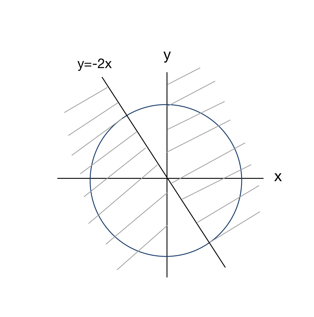
Under the following conditions, we will have (14) larger than 0.

{yβ‰₯βˆ’2​x​if ​x>0y<βˆ’2​x​if ​x<0cases𝑦2π‘₯ifΒ π‘₯0missing-subexpression𝑦2π‘₯ifΒ π‘₯0missing-subexpression\left\{\begin{array}[]{lr}y\geq-2x\;\;\;\text{if\;}x>0\\ y<-2x\;\;\;\text{if\;}x<0\end{array}\right.

The shadow region in the following figure shows the area satisfying the above condition, which indicates a large probability, around 5/6 (more accurately, 1-2*arctan (0.5)) of Q2βˆ’Q1>0subscript𝑄2subscript𝑄10Q_{2}-Q_{1}>0. In other words, there is a probability around 5/6 that SPSA with Bernoulli outperforms RDSA with Gaussian.
Refer to caption
Figure 1: Region of equation (14) being larger than 0

Then we are going to consider the high-dim case. Denote:

Q1=(𝒖1+𝒖2)T​𝑺​(𝒖1+𝒖2),Q2=(3​𝒖1+𝒖2)T​𝑺​(3​𝒖1+𝒖2).formulae-sequencesubscript𝑄1superscriptsubscript𝒖1subscript𝒖2𝑇𝑺subscript𝒖1subscript𝒖2subscript𝑄2superscript3subscript𝒖1subscript𝒖2𝑇𝑺3subscript𝒖1subscript𝒖2\displaystyle\begin{split}&{Q}_{1}=(\bm{u}_{1}+\bm{u}_{2})^{T}\bm{S}(\bm{u}_{1}+\bm{u}_{2}),\\ &{Q}_{2}=(3\bm{u}_{1}+\bm{u}_{2})^{T}\bm{S}(3\bm{u}_{1}+\bm{u}_{2}).\end{split}

We would like to compare Q2,Q1subscript𝑄2subscript𝑄1Q_{2},Q_{1}. Similar to the scalar case, set 𝒙=𝑺1/2​𝒖1,π’š=𝑺1/2​𝒖2.formulae-sequence𝒙superscript𝑺12subscript𝒖1π’šsuperscript𝑺12subscript𝒖2\bm{x}=\bm{S}^{1/2}\bm{u}_{1},\bm{y}=\bm{S}^{1/2}\bm{u}_{2}. Then consider:

𝒛=Q2βˆ’Q1𝒛subscript𝑄2subscript𝑄1\displaystyle\bm{z}=Q_{2}-Q_{1} (17)
=(3​𝒙+π’š)T​(3​𝒙+π’š)βˆ’(𝒙+π’š)T​(𝒙+π’š)absentsuperscript3π’™π’šπ‘‡3π’™π’šsuperscriptπ’™π’šπ‘‡π’™π’š\displaystyle=(3\bm{x}+\bm{y})^{T}(3\bm{x}+\bm{y})-(\bm{x}+\bm{y})^{T}(\bm{x}+\bm{y}) (18)
=4​(2​𝒙T​𝒙+𝒙Tβ€‹π’š)absent42superscript𝒙𝑇𝒙superscriptπ’™π‘‡π’š\displaystyle=4(2\bm{x}^{T}\bm{x}+\bm{x}^{T}\bm{y}) (19)
=4​𝒙T​(2​𝒙+π’š)absent4superscript𝒙𝑇2π’™π’š\displaystyle=4\bm{x}^{T}(2\bm{x}+\bm{y}) (20)

Here we consider a simple case to have a straightforward understanding. Set 𝒙,π’šπ’™π’š\bm{x},\bm{y} to be two independent random variables with uniform symmetrical distribution (i.e. 𝒙=(x1,x2,…,xp)T,π’š=(y1,y2,…,yp)T,xi∼i.i.dU​(βˆ’a,a),yi∼i.i.dU​(βˆ’b,b)formulae-sequence𝒙superscriptsubscriptπ‘₯1subscriptπ‘₯2…subscriptπ‘₯𝑝𝑇formulae-sequenceπ’šsuperscriptsubscript𝑦1subscript𝑦2…subscript𝑦𝑝𝑇formulae-sequencesuperscriptsimilar-toi.i.dsubscriptπ‘₯π‘–π‘ˆπ‘Žπ‘Žsuperscriptsimilar-toi.i.dsubscriptπ‘¦π‘–π‘ˆπ‘π‘\bm{x}=(x_{1},x_{2},...,x_{p})^{T},\bm{y}=(y_{1},y_{2},...,y_{p})^{T},\;x_{i}\stackrel{{\scriptstyle\text{i.i.d}}}{{\sim}}U(-a,a),y_{i}\stackrel{{\scriptstyle\text{i.i.d}}}{{\sim}}U(-b,b)) and 𝑺𝑺\bm{S} to be the identical matrix. Then we have:

E​(𝒙T​𝒙)=E​(βˆ‘i=1pxi2)=βˆ‘i=1pE​(xi2)=βˆ‘i=1pV​a​r​(xi)=a2​p3.𝐸superscript𝒙𝑇𝒙𝐸subscriptsuperscript𝑝𝑖1subscriptsuperscriptπ‘₯2𝑖subscriptsuperscript𝑝𝑖1𝐸subscriptsuperscriptπ‘₯2𝑖subscriptsuperscript𝑝𝑖1π‘‰π‘Žπ‘Ÿsubscriptπ‘₯𝑖superscriptπ‘Ž2𝑝3\displaystyle E(\bm{x}^{T}\bm{x})=E\left(\sum\limits^{p}_{i=1}x^{2}_{i}\right)=\sum\limits^{p}_{i=1}E(x^{2}_{i})=\sum\limits^{p}_{i=1}Var(x_{i})=\dfrac{a^{2}p}{3}.
E​(𝒙Tβ€‹π’š)=E​(βˆ‘i=1pxi​yi)=βˆ‘i=1pE​(xi)​E​(yi)=0.(due to the independence)formulae-sequence𝐸superscriptπ’™π‘‡π’šπΈsubscriptsuperscript𝑝𝑖1subscriptπ‘₯𝑖subscript𝑦𝑖subscriptsuperscript𝑝𝑖1𝐸subscriptπ‘₯𝑖𝐸subscript𝑦𝑖0due to the independence\displaystyle E(\bm{x}^{T}\bm{y})=E\left(\sum\limits^{p}_{i=1}x_{i}y_{i}\right)=\sum\limits^{p}_{i=1}E(x_{i})E(y_{i})=0.\;\;\;(\text{due\;to\;the\;independence})
E​(𝒛)=8​E​(𝒙T​𝒙)+4​E​(𝒙Tβ€‹π’š)=8​a2​p3.𝐸𝒛8𝐸superscript𝒙𝑇𝒙4𝐸superscriptπ’™π‘‡π’š8superscriptπ‘Ž2𝑝3\displaystyle E(\bm{z})=8E(\bm{x}^{T}\bm{x})+4E(\bm{x}^{T}\bm{y})=\dfrac{8a^{2}p}{3}.

Furthermore, we use one-sided version of Chebyshev inequality to see the probability that 𝒛≀0𝒛0\bm{z}\leq 0, which indicates Q2≀Q1subscript𝑄2subscript𝑄1Q_{2}\leq Q_{1}. The inequality states that P​(Xβ‰₯c)≀V​a​r​(X)/[V​a​r​(X)+c2]π‘ƒπ‘‹π‘π‘‰π‘Žπ‘Ÿπ‘‹delimited-[]π‘‰π‘Žπ‘Ÿπ‘‹superscript𝑐2P(X\geq c)\leq Var(X)/[Var(X)+c^{2}]. In our case, the inequality is in the form of:

P​[(βˆ’π’›+E​(𝒛))β‰₯E​(𝒛)]𝑃delimited-[]𝒛𝐸𝒛𝐸𝒛\displaystyle P[(-\bm{z}+E(\bm{z}))\geq E(\bm{z})] ≀V​a​r​[βˆ’π’›+E​(𝒛)]V​a​r​[βˆ’π’›+E​(𝒛)]+[E​(𝒛)]2absentπ‘‰π‘Žπ‘Ÿdelimited-[]π’›πΈπ’›π‘‰π‘Žπ‘Ÿdelimited-[]𝒛𝐸𝒛superscriptdelimited-[]𝐸𝒛2\displaystyle\leq\dfrac{Var[-\bm{z}+E(\bm{z})]}{Var[-\bm{z}+E(\bm{z})]+[E(\bm{z})]^{2}} (21)
=V​a​r​(𝒛)V​a​r​(𝒛)+[E​(𝒛)]2.absentπ‘‰π‘Žπ‘Ÿπ’›π‘‰π‘Žπ‘Ÿπ’›superscriptdelimited-[]𝐸𝒛2\displaystyle=\dfrac{Var(\bm{z})}{Var(\bm{z})+[E(\bm{z})]^{2}}. (22)

To simplify the calculation, we set xi∼i.i.dU​(βˆ’a,a),yi∼i.i.dU​(βˆ’a,a)formulae-sequencesuperscriptsimilar-toi.i.dsubscriptπ‘₯π‘–π‘ˆπ‘Žπ‘Žsuperscriptsimilar-toi.i.dsubscriptπ‘¦π‘–π‘ˆπ‘Žπ‘Žx_{i}\stackrel{{\scriptstyle\text{i.i.d}}}{{\sim}}U(-a,a),y_{i}\stackrel{{\scriptstyle\text{i.i.d}}}{{\sim}}U(-a,a). Then we have:

V​a​r​(𝒛)π‘‰π‘Žπ‘Ÿπ’›\displaystyle Var(\bm{z}) =V​a​r​(8​𝒙T​𝒙)+V​a​r​(4​𝒙Tβ€‹π’š)+C​o​v​(8​𝒙T​𝒙,4​𝒙Tβ€‹π’š)absentπ‘‰π‘Žπ‘Ÿ8superscriptπ’™π‘‡π’™π‘‰π‘Žπ‘Ÿ4superscriptπ’™π‘‡π’šπΆπ‘œπ‘£8superscript𝒙𝑇𝒙4superscriptπ’™π‘‡π’š\displaystyle=Var(8\bm{x}^{T}\bm{x})+Var(4\bm{x}^{T}\bm{y})+Cov(8\bm{x}^{T}\bm{x},4\bm{x}^{T}\bm{y})
=64​V​a​r​(βˆ‘i=1pxi2)+16​V​a​r​(βˆ‘i=1pxi​yi)=64​p​a45+16​p​a49=16Γ—41​p​a445.absent64π‘‰π‘Žπ‘Ÿsubscriptsuperscript𝑝𝑖1subscriptsuperscriptπ‘₯2𝑖16π‘‰π‘Žπ‘Ÿsubscriptsuperscript𝑝𝑖1subscriptπ‘₯𝑖subscript𝑦𝑖64𝑝superscriptπ‘Ž4516𝑝superscriptπ‘Ž491641𝑝superscriptπ‘Ž445\displaystyle=64Var\left(\sum\limits^{p}_{i=1}x^{2}_{i}\right)+16Var\left(\sum\limits^{p}_{i=1}x_{i}y_{i}\right)=\dfrac{64pa^{4}}{5}+\dfrac{16pa^{4}}{9}=16\times\dfrac{41pa^{4}}{45}.

Plug it into the inequality (20), it looks like:

P(𝒛≀0))\displaystyle P(\bm{z}\leq 0)) ≀V​a​r​(𝒛)V​a​r​(𝒛)+[E​(𝒛)]2absentπ‘‰π‘Žπ‘Ÿπ’›π‘‰π‘Žπ‘Ÿπ’›superscriptdelimited-[]𝐸𝒛2\displaystyle\leq\dfrac{Var(\bm{z})}{Var(\bm{z})+[E(\bm{z})]^{2}} (23)
=16Γ—41​p​a44516Γ—41​p​a445+64​p2​a49absent1641𝑝superscriptπ‘Ž4451641𝑝superscriptπ‘Ž44564superscript𝑝2superscriptπ‘Ž49\displaystyle=\dfrac{16\times\dfrac{41pa^{4}}{45}}{16\times\dfrac{41pa^{4}}{45}+\dfrac{64p^{2}a^{4}}{9}} (24)
=4141+20​p.absent414120𝑝\displaystyle=\dfrac{41}{41+20p}. (25)

Inequality (23) shows that as the dimension p𝑝p increases, the probability of 𝒛≀0𝒛0\bm{z}\leq 0 decreases. Here we make a simulation by setting a range of dimension from 1 to 10 and then take 100,000 independent trials to calculate the probability, i.e. P​(𝒛≀0)𝑃𝒛0P(\bm{z}\leq 0) with 𝑺=𝑰;𝒖1​i∼i.i.dU​(βˆ’100,100);𝒖2​i∼i.i.dU​(βˆ’100,100),i=1,2,…,pformulae-sequence𝑺𝑰formulae-sequencesuperscriptsimilar-toi.i.dsubscript𝒖1π‘–π‘ˆ100100formulae-sequencesuperscriptsimilar-toi.i.dsubscript𝒖2π‘–π‘ˆ100100𝑖12…𝑝\bm{S}=\bm{I};\;\bm{u}_{1i}\stackrel{{\scriptstyle\text{i.i.d}}}{{\sim}}U(-100,100);\;\bm{u}_{2i}\stackrel{{\scriptstyle\text{i.i.d}}}{{\sim}}U(-100,100),\;i=1,2,...,p. The result is shown in the following Table 3, demonstrating a decreasing trend when the dimension gets large. Also, it shows consistency with the conclusion in the scalar case, namely, when p=1,P​(z≀0)β‰ˆ16formulae-sequence𝑝1𝑃𝑧016p=1,P(z\leq 0)\approx\dfrac{1}{6}.

Table 3: Relationship Between Dimension and P​(𝒛≀0)𝑃𝒛0P(\bm{z}\leq 0)
Dim 1 2 3 4 5
𝑷​(𝒛≀0)𝑷𝒛0\bm{P}(\bm{z}\leq 0) 0.12546 0.0336 0.00932 0.00252 0.00071
Dim 6 7 8 9 10
𝑷​(𝒛≀0)𝑷𝒛0\bm{P}(\bm{z}\leq 0) 0.00024 9Γ—10βˆ’59superscript1059\times 10^{-5} 3Γ—10βˆ’53superscript1053\times 10^{-5} 0 0

As Table 3 indicates, if we consider those high-dimension cases, there will be a tiny probability that Q2≀Q1subscript𝑄2subscript𝑄1Q_{2}\leq Q_{1}, i.e. SPSA with Bernoulli will highly probably beat RDSA with Gaussian from the perspective of a smaller MSE. However, it should be noticed that the above case is based on a simple simulated setting, which aims at providing an intuitive view at the comparison of Gaussian and Bernoulli.

In the next section, we will show how Proposition 3 works more specifically by some numerical experiments.

4 Numerical Experiment

4.1 Numerical Example 1

Consider the loss function [3]:

L​(ΞΈ)=β€–ΞΈβ€–2+βˆ‘i=1peti/p,𝐿θsuperscriptnormΞΈ2superscriptsubscript𝑖1𝑝superscript𝑒subscript𝑑𝑖𝑝L(\uptheta)=||\uptheta||^{2}+\sum\limits_{i=1}^{p}e^{t_{i}/p},

where 𝛉=[t1,t2,…,tp]T𝛉superscriptsubscript𝑑1subscript𝑑2…subscript𝑑𝑝𝑇\bm{\uptheta}=[t_{1},t_{2},...,t_{p}]^{T} and the minimum occurs at π›‰βˆ—superscript𝛉\bm{\uptheta}^{*} with each component βˆ’0.0330.033-0.033, such that L​(π›‰βˆ—)=29.99994𝐿superscript𝛉29.99994L(\bm{\uptheta}^{*})=29.99994. This is a convex function with third-derivative being nonzero and cross third-derivative being zero. Namely, in our case, we have 𝒖2=𝟎subscript𝒖20\bm{u}_{2}=\bm{0} and 𝒖1>𝟎subscript𝒖10\bm{u}_{1}>\bm{0}. So according to the Corollary in Proposition 3, SPSA with Bernoulli has lower MSE than RDSA with Gaussian.

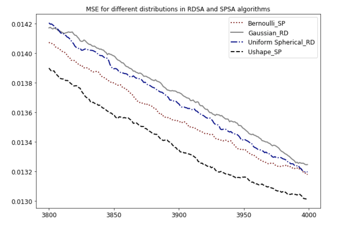
Let p=30𝑝30p=30 and take 100 independent trials, each with 3000 iterations. Results are presented in Fig 2 and Table 4. We assume the noise term has distribution N​(0,0.01)𝑁00.01N(0,0.01) and gain sequence as ak=0.05/(k+1)0.602,ck=0.3/(k+1)0.101formulae-sequencesubscriptπ‘Žπ‘˜0.05superscriptπ‘˜10.602subscriptπ‘π‘˜0.3superscriptπ‘˜10.101a_{k}=0.05/(k+1)^{0.602},\,c_{k}=0.3/(k+1)^{0.101}. Set the initial point 𝛉^0=[1,1,…,1]Tsubscript^𝛉0superscript11…1𝑇\hat{\bm{\uptheta}}_{0}=[1,1,...,1]^{T}. The results are shown below. The lowest MSE is highlighted in bold in Table 4 and other numerical results below.
Refer to caption
Figure 2: Mean Square Error, computed as an average over 100 trials, plotted the last 200 iterations for different random perturbation distributions
Table 4: MSE and confidence interval in SPSA and RDSA with different perturbations with same gain sequences in all algorithms
Perturbation MSE 95% CI
Bernoulli SP 0.01318 [0.01281, 0.01354]
U-shape(π’™πŸπŸŽsuperscript𝒙10\bm{x^{10}}) SP 0.01301 [0.01266, 0.01336]
Gaussian RD 0.01325 [0.01290, 0.01359]
Uniformly Spherical RD 0.01319 [0.01285, 0.01355]

The experimental result shows consistency with the Proposition 3. The confidence intervals show overlap among the four and then we conduct the two-sample t𝑑t-test between the Bernoulli and Gaussian cases and obtain the p𝑝p-value 0.35982, which is larger than the common threshold, 0.05, indicating that the difference is not statistically significant. The reason is that in this case, the D𝐷D value (shown in the Table 2) is much larger than the term 𝒖1T​𝑺​𝒖1superscriptsubscript𝒖1𝑇𝑺subscript𝒖1\bm{u}_{1}^{T}\bm{Su}_{1} so that it dominates the whole MSE value. So the MSE of SPSA with Bernoulli is slightly smaller than that of RDSA with Gaussian. Moreover, we notice that the MSE of U-Shape distributed perturbation is the smallest one which can also be explained by the 0.9 in front of the value D𝐷D.

4.2 Numerical Example 2

Consider the Ackley Function with dimension p=30𝑝30p=30:

L​(𝛉)𝐿𝛉\displaystyle L(\bm{\uptheta}) =βˆ’aΓ—exp​(βˆ’b​130β€‹βˆ‘i=1dti2)βˆ’exp​(130β€‹βˆ‘i=1dcos​(c​ti))+a+e,absentπ‘Žexp𝑏130subscriptsuperscript𝑑𝑖1subscriptsuperscript𝑑2𝑖exp130subscriptsuperscript𝑑𝑖1cos𝑐subscriptπ‘‘π‘–π‘Žπ‘’\displaystyle=-a\times\text{exp}\left(-b\sqrt{\dfrac{1}{30}\sum\limits^{d}_{i=1}t^{2}_{i}}\right)-\text{exp}\left(\dfrac{1}{30}\sum\limits^{d}_{i=1}\text{cos}(ct_{i})\right)+a+e,

where a=20,b=0.2,c=2​π,𝛉=[t1,t2,…,t30]formulae-sequenceπ‘Ž20formulae-sequence𝑏0.2formulae-sequence𝑐2πœ‹π›‰subscript𝑑1subscript𝑑2…subscript𝑑30a=20,b=0.2,c=2\pi,\,\bm{\uptheta}=[t_{1},t_{2},...,t_{30}] and L​(𝛉)=0𝐿𝛉0L(\bm{\uptheta})=0 at π›‰βˆ—=[1,1,…,1]T.superscript𝛉superscript11…1𝑇\bm{\uptheta}^{*}=[1,1,...,1]^{T}. Here, we assume the noise term has distribution N​(0,0.01)𝑁00.01N(0,0.01) and gain sequence as ak=0.02/(k+1+A)0.602,A=10,ck=0.2/(k+1)0.101formulae-sequencesubscriptπ‘Žπ‘˜0.02superscriptπ‘˜1𝐴0.602formulae-sequence𝐴10subscriptπ‘π‘˜0.2superscriptπ‘˜10.101a_{k}=0.02/(k+1+A)^{0.602},\;A=10,\,c_{k}=0.2/(k+1)^{0.101}. Set the initial point 𝛉^0=[0.2,0.2,…,0.2]Tsubscript^𝛉0superscript0.20.2…0.2𝑇\hat{\bm{\uptheta}}_{0}=[0.2,0.2,...,0.2]^{T}.

In this case, there are no cross-third derivatives, i.e.  𝒖2=𝟎subscript𝒖20\bm{u}_{2}=\bm{0}. By Proposition 3, SPSA with Bernoulli would have smaller MSE value than RDSA with Gaussian. Take 100 independent trials, each with 5000 iterations. The results are shown in Fig 3 and Table 5:
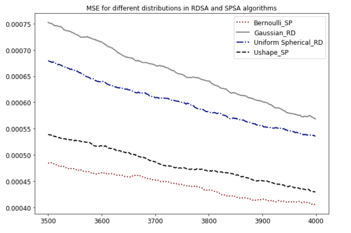
Refer to caption
Figure 3: Mean Square Error, computed as an average over 100 trials, plotted the last 500 iterations for different random perturbation distributions
Table 5: MSE and its Confidence Interval in SPSA and RDSA with different perturbations with same gain sequences in all algorithms
Perturbation MSE 95% CI
Bernoulli SP 0.00041 [0.00038, 0.00044]
U-shape (x10superscriptπ‘₯10x^{10}) SP 0.00043 [0.00041, 0.00045]
Uniformly Spherical RD 0.00054 [0.00051, 0.00056]
Gaussian RD 0.00057 [0.00054, 0.00060]

The MSE value of SPSA with Bernoulli case is lower than that of RDSA with Gaussian case, which is accordant with the Proposition 3. Notice that the confidence interval of the two cases does not overlap and we take the two-sample t𝑑t-test between them and gain the p𝑝p-value 5.96Γ—10βˆ’135.96superscript10135.96\times 10^{-13}, which indicates that the difference is significant.

4.3 Numerical Example 3

To give a more specific example. Consider the skewed-quartic function:

L​(𝛉)=𝛉T​𝑩T​𝑩​𝛉+0.1β€‹βˆ‘i=1p(𝑩​𝛉)i3+0.01β€‹βˆ‘i=1p(𝑩​𝛉)i4.𝐿𝛉superscript𝛉𝑇superscript𝑩𝑇𝑩𝛉0.1subscriptsuperscript𝑝𝑖1subscriptsuperscript𝑩𝛉3𝑖0.01subscriptsuperscript𝑝𝑖1subscriptsuperscript𝑩𝛉4𝑖L({\bm{\uptheta}})={\bm{\uptheta}}^{T}{\bm{B}}^{T}{\bm{B\uptheta}}+0.1\sum\limits^{p}_{i=1}({\bm{B\uptheta}})^{3}_{i}+0.01\sum\limits^{p}_{i=1}({\bm{B\uptheta}})^{4}_{i}.

4.3.1 Optimal Gain Sequence Searching

We consider searching the β€˜optimal gain sequence’ for aksubscriptπ‘Žπ‘˜a_{k} and cksubscriptπ‘π‘˜c_{k} in the gain sequence with the smallest MSE value, i.e. set ak=a/(k+A+1)Ξ±,ck=c/(k+1)Ξ³formulae-sequencesubscriptπ‘Žπ‘˜π‘Žsuperscriptπ‘˜π΄1𝛼subscriptπ‘π‘˜π‘superscriptπ‘˜1𝛾a_{k}=a/(k+A+1)^{\alpha},\;c_{k}=c/(k+1)^{\gamma} and keep A=10𝐴10A=10. Then set the search range of aπ‘Ža and c𝑐c to be 0.1 to 1, with interval 0.02 and pick the sequence leading to the lowest MSE value. The β€˜optimal gain sequence’ for each case has been listed in Table 6. Particularly, in order to satisfy that π›β‰ πŸŽπ›0\bm{\upmu}\neq\bm{0} in (9), we set Ξ±=0.606,Ξ³=0.101formulae-sequenceΞ±0.606Ξ³0.101\upalpha=0.606,\upgamma=0.101 in the gain sequence.

Table 6: Optimal Gain Sequence for Algorithms with distinct Perturbations
Perturbation aksubscriptπ‘Žπ‘˜a_{k} cksubscriptπ‘π‘˜c_{k}
Bernoulli SP 0.12/(k+11)0.6060.12superscriptπ‘˜110.6060.12/(k+11)^{0.606} 0.8/(k+1)0.1010.8superscriptπ‘˜10.1010.8/(k+1)^{0.101}
U-shape (x10superscriptπ‘₯10x^{10}) SP 0.1/(k+11)0.6060.1superscriptπ‘˜110.6060.1/(k+11)^{0.606} 0.48/(k+1)0.1010.48superscriptπ‘˜10.1010.48/(k+1)^{0.101}
Uniformly Spherical RD 0.1/(k+11)0.6060.1superscriptπ‘˜110.6060.1/(k+11)^{0.606} 0.42/(k+1)0.1010.42superscriptπ‘˜10.1010.42/(k+1)^{0.101}
Gaussian RD 0.1/(k+11)0.606superscriptπ‘˜110.606(k+11)^{0.606} 0.58/(k+1)0.1010.58superscriptπ‘˜10.1010.58/(k+1)^{0.101}

4.3.2 Further Comparison

In order to conduct a further comparison of the performance of RDSA and SPSA algorithm, as well as work in connection with our previous theoretical calculation, we are going to apply the optimal gain sequence for each distribution to the other three distributions and see the result. That is, in 1)-4) below, we, in turn, pick one of the pairs {ak,cksubscriptπ‘Žπ‘˜subscriptπ‘π‘˜a_{k},c_{k}} in Table 6 and run all four methods at the chosen gain sequence. This will demonstrate each method in its best configuration. Then we mainly focus on the Bernoulli and Gaussian to see their comparison.

  • 1)

    Apply the optimal gain sequence for Bernoulli, i.e. set ak=0.12/((k+11)0.606),ck=0.8/((k+1)0.101a_{k}=0.12/((k+11)^{0.606}),c_{k}=0.8/((k+1)^{0.101} for the four methods. The result is shown in Fig 4 and Table 7.
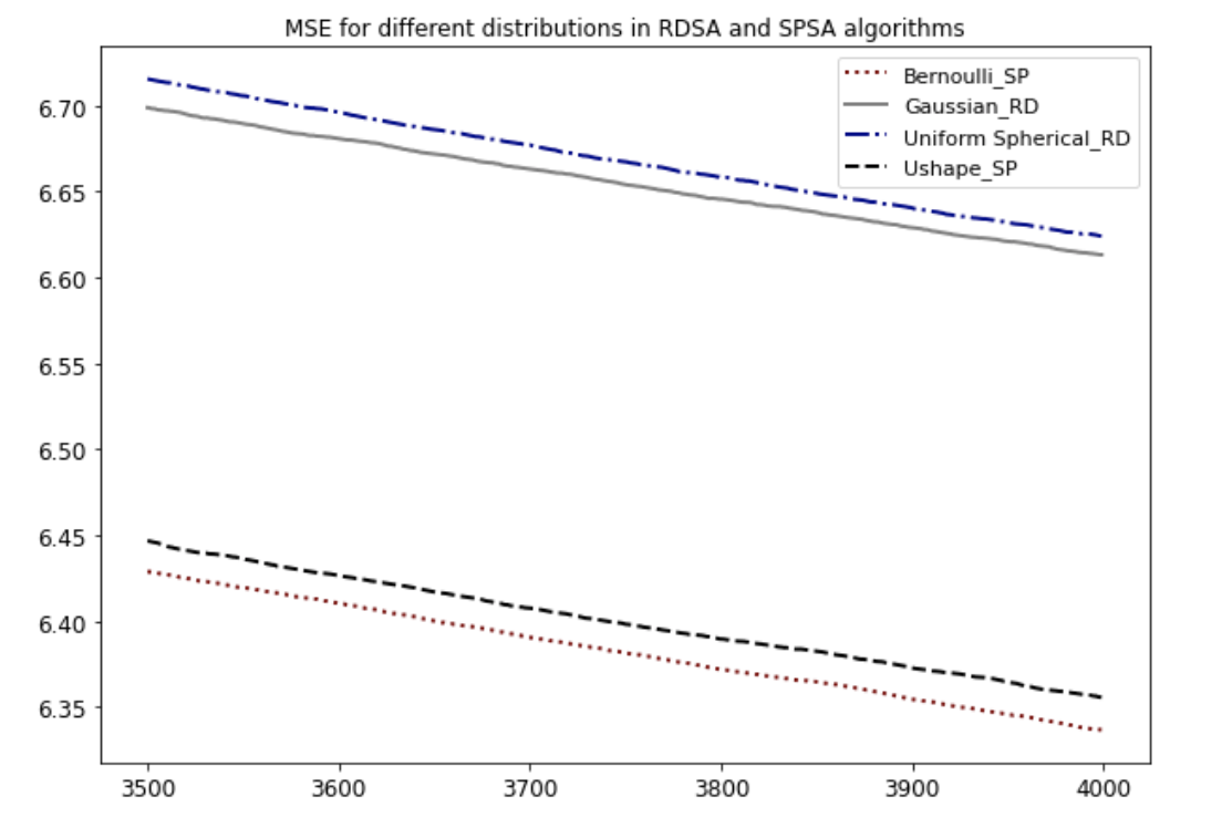
    Refer to caption
    Figure 4: Mean Square Error, computed as an average over 100 trials each of 4000 iterations with the optimal gain for Bernoulli distributed perturbation in SPSA, plotted the last 500 iterations for different random direction distributions
    Table 7: MSE for Skewed Quartic Loss Function and its Confidence Interval
    (Gain Sequence ak=0.12/((k+11)0.606),ck=0.8/((k+1)0.101a_{k}=0.12/((k+11)^{0.606}),c_{k}=0.8/((k+1)^{0.101})
    Perturbation MSE 95% CI
    Bernoulli SP 6.3368 [6.0959, 6.5778]
    U-shape (x10superscriptπ‘₯10x^{10}) SP 6.3557 [6.0536, 6.6579]
    Uniformly Spherical RD 6.6240 [6.3064, 6.9416]
    Gaussian RD 6.6132 [6.2637, 6.9626]

    We find that the Bernoulli performs the best, then the U-shape, Uniformly Spherical and Gaussian being the worst one. It is accordant with the previous Table 2. Also, we find that the 95% confidence interval of Bernoulli and Gaussian does not overlap. The two-sample test between Bernoulli and Gaussian produces the p𝑝p-value 0.0040573, indicating that the difference is significant.

  • 2)

    Apply the optimal gain sequence for U-shape, i.e. set ak=0.1/((k+11)0.606),ck=0.48/((k+1)0.101a_{k}=0.1/((k+11)^{0.606}),c_{k}=0.48/((k+1)^{0.101} for the four methods. The result is shown in Fig 5 and Table 8.
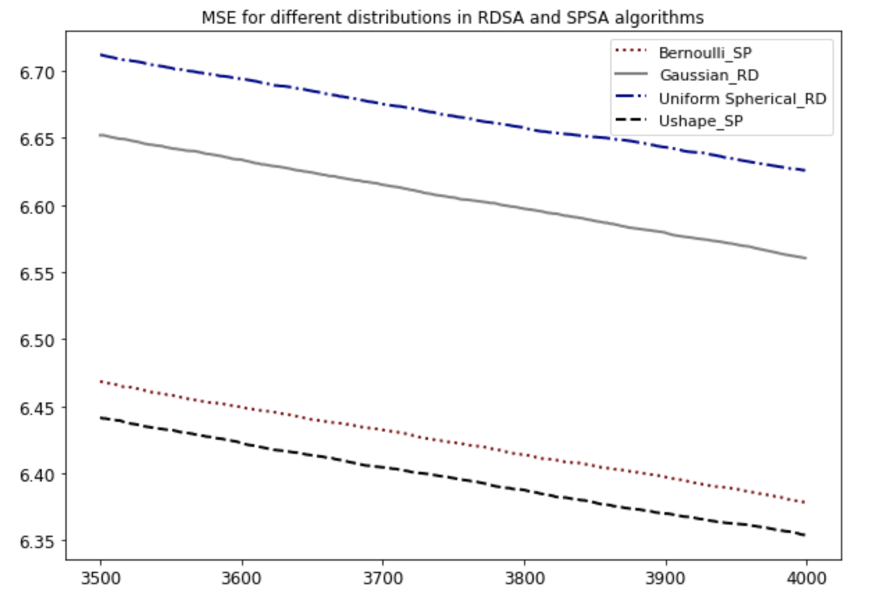
    Refer to caption
    Figure 5: Mean Square Error, computed as an average over 100 trials each of 4000 iterations with the optimal gain for U-shape in SPSA, plotted the last 500 iterations for different random direction distributions
    Table 8: MSE for Skewed Quartic Loss Function and its Confidence Interval
    (Gain Sequence ak=0.1/((k+11)0.606),ck=0.48/((k+1)0.101a_{k}=0.1/((k+11)^{0.606}),c_{k}=0.48/((k+1)^{0.101})
    Perturbation MSE 95% CI
    Bernoulli SP 6.3784 [6.1038, 6.6531]
    U-shape(π’™πŸπŸŽsuperscript𝒙10\bm{x^{10}}) SP 6.3540 [6.0761, 6.6320]
    Uniformly Spherical RD 6.6257 [6.3150, 6.9365]
    Gaussian RD 6.5604 [6.2803, 6.8406]
  • 3)

    Apply the optimal gain sequence for Uniform Spherical, i.e. set ak=0.1/((k+11)0.606),ck=0.42/((k+1)0.101a_{k}=0.1/((k+11)^{0.606}),c_{k}=0.42/((k+1)^{0.101} for the four methods. The result is shown in Fig 6 and Table 9.
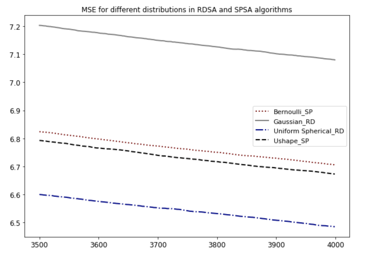
    Refer to caption
    Figure 6: Mean Square Error, computed as an average over 100 trials each of 4000 iterations with the optimal gain for Uniform Spherical in RDSA, plotted the last 500 iterations for different random direction distributions
    Table 9: MSE for Skewed Quartic Loss Function and its Confidence Interval
    (Gain Sequence ak=0.1/((k+11)0.606),ck=0.42/((k+1)0.101a_{k}=0.1/((k+11)^{0.606}),c_{k}=0.42/((k+1)^{0.101})
    Perturbation MSE 95% CI
    Bernoulli SP 6.7323 [6.4523,7.0123]
    U-shape (x10superscriptπ‘₯10x^{10}) SP 6.7012 [6.4212,6.9812]
    Uniformly Spherical RD 6.4436 [6.1636,6.7236]
    Gaussian RD 7.0789 [6.7889,7.3689]

    We find that under such gain sequence, the Uniform Spherical performs the best and Bernoulli still outperforms Gaussian, consistent with the Table 2. We then conduct the two-sample t𝑑t-test between Bernoulli and Gaussian and obtain the p𝑝p-value 0.121487, indicating that the difference is not statistically significant.

  • 4)

    Apply the optimal gain sequence for Gaussian, i.e. set ak=0.1/((k+11)0.606),ck=0.58/((k+1)0.101a_{k}=0.1/((k+11)^{0.606}),c_{k}=0.58/((k+1)^{0.101} for the four methods. The result is shown in Fig 7 and Table 10.
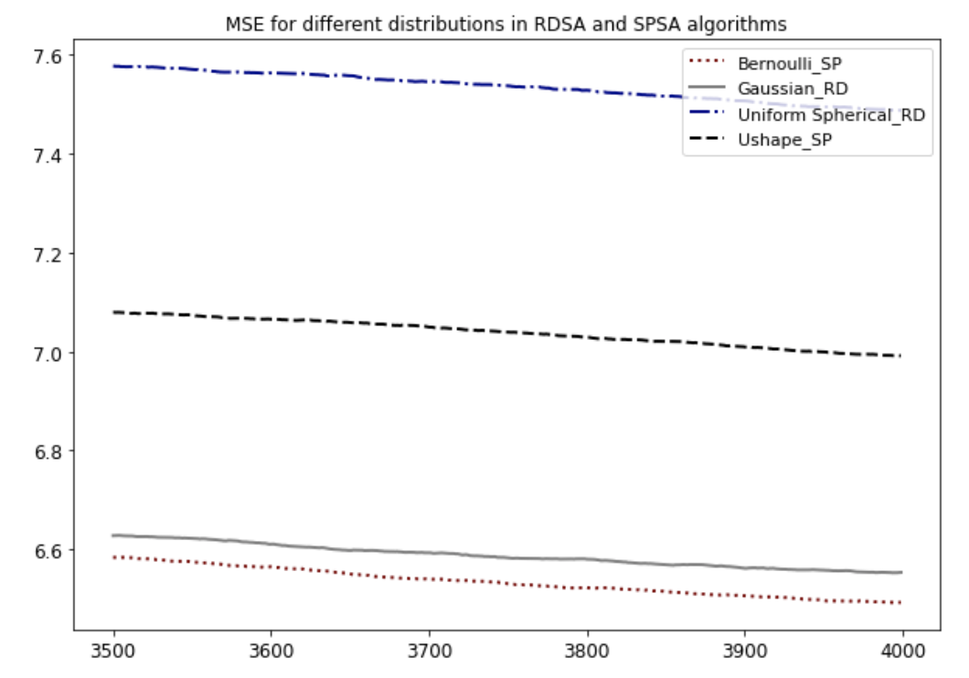
    Refer to caption
    Figure 7: Mean Square Error, computed as an average over 100 trials each of 4000 iterations with the optimal gain for Gaussian distributed perturbation in RDSA, plotted the last 500 iterations for different random direction distributions
    Table 10: MSE for Skewed Quartic Loss Function and its Confidence Interval
    (Gain Sequence ak=0.1/((k+11)0.606),ck=0.58/((k+1)0.101a_{k}=0.1/((k+11)^{0.606}),c_{k}=0.58/((k+1)^{0.101})
    Perturbation MSE 95% CI
    Bernoulli SP 6.4928 [6.2314, 6.7542]
    U-shape (x10superscriptπ‘₯10x^{10}) SP 6.9915 [6.7374, 7.2456]
    Uniformly Spherical RD 7.4873 [7.1479, 7.8267]
    Gaussian RD 6.5534 [6.2897, 6.8171]

In this case, although the optimal gain sequence of Gaussian has been applied and the Gaussian reaches its lowest MSE, it is still smaller than the MSE of Bernoulli, which can be a strong support for the theoretical conclusion shown in Proposition 3. The two-sample test between Bernoulli and Gaussian produces the p𝑝p-value 0.2431523, indicating that the difference is not statistically significant.

From above four experiments, all the four algorithms show their best performance from the perspective of a lowest MSE when their optimal gain sequence is applied. The tables show that no matter in which case, SPSA with Bernoulli beats RDSA with Gaussian, showing consistency with Proposition 3.

5 Conclusion

This paper provides a strict derivation for several essential terms in the RDSA algorithm and presents a comparison of the asymptotic MSE between RDSA and SPSA. Furthermore, this paper presents specific conditions under which SPSA with Bernoulli perturbation works better in the MSE sense than RDSA with Gaussian perturbation, which may provide practitioners a general guidance in the practical cases. In particular, it is found that SPSA outperforms RDSA across the large majority of implementation cases with different gain sequences and types of loss functions.

There are several directions for future research. First, we can consider extra types of random directions with different distributions. Second, more work related to robustness and relative efficiency would be useful. Third, since this paper mainly focuses on Bernoulli and Gaussian cases, more general cases could be considered for the comparison of MSE between SPSA and RDSA. It would also be of interest to carry out a comparison such as that above for both second-order or non-continuous versions of SPSA and RDSA, such as presented in [16], [19], [17], [21], and [10], and constant-gain (step size) versions, such as in [8], [20], and [11].

References

  • [1] Shalabh Bhatnagar, Harshika Prasad, and L.Β A. Prashanth. Stochastic recursive algorithms for optimization. Simultaneous perturbation methods, volume 434. Jan 2013.
  • [2] A.Β Blakney and J.Β Zhu. A comparison of the finite difference and simultaneous perturbation gradient estimation methods with noisy function evaluations. In 2019 53rd Annual Conference on Information Sciences and Systems (CISS), pages 1–6, 2019.
  • [3] D.Β C. Chin. Comparative study of stochastic algorithms for system optimization based on gradient approximations. IEEE Transactions on Systems, Man, and Cybernetics, Part B (Cybernetics), 27(2):244–249, 1997.
  • [4] KarlaΒ HernΓ‘ndez Cuevas. Cyclic stochastic optimization: Generalizations, convergence, and applications in multi-agent systems, PhD Dissertation, Johns Hopkins University, https://arxiv.org/abs/1707.06700, 2017.
  • [5] Vaclav Fabian. On asymptotic normality in stochastic approximation. The Annals of Mathematical Statistics, 39(4):1327–1332, 1968.
  • [6] Karla HernΓ‘ndez and J.Β C. Spall. Generalization of a result of Fabian on the asymptotic normality of stochastic approximation. Automatica, 99:420 – 424, 2019.
  • [7] J.L.Doob. Stochastic Process. New York: Wiley, 1953.
  • [8] Itsuro Kajiwara, Keiichiro Furuya, and Shinichi Ishizuka. Experimental verification of a real-time tuning method of a model-based controller by perturbations to its poles. Mechanical Systems and Signal Processing, 107:396–408, 2018.
  • [9] H.Β J. Kusher and G.Β Yin. Random directions methods in stochastic approximation. In Proceedings of the 36th IEEE Conference on Decision and Control, pages 3430–3435 vol.4, 1997.
  • [10] L.Β A. Prashanth, S.Β Bhatnagar, M.Β Fu, and S.Β Marcus. Adaptive system optimization using random directions stochastic approximation. IEEE Transactions on Automatic Control, 62(5):2223–2238, 2017.
  • [11] A.Β Ramaswamy. DSPG: Decentralized simultaneous perturbations gradient descent scheme. In 2020 28th Euromicro International Conference on Parallel, Distributed and Network-Based Processing (PDP), pages 54–62, Los Alamitos, CA, USA, Mar 2020. IEEE Computer Society.
  • [12] J.Β C. Spall. Multivariate stochastic approximation using a simultaneous perturbation gradient approximation. IEEE Transactions on Automatic Control, 37(3):332–341, 1992.
  • [13] J.Β C. Spall. Developments in stochastic optimization algorithms with gradient approximations based on function measurements. In Proceedings of Winter Simulation Conference, pages 207–214, 1994.
  • [14] J.Β C. Spall. An overview of the simultaneous perturbation method for efficient optimization. Johns Hopkins APL Technical Digest, 19:482–492, 1998.
  • [15] J.Β C. Spall. Introduction to stochastic search and optimization: estimation, simulation, and control, volumeΒ 65. John Wiley & Sons, 2005.
  • [16] J.Β C. Spall. Feedback and weighting mechanisms for improving Jacobian estimates in the adaptive simultaneous perturbation algorithm. IEEE Transactions on Automatic Control, 54(6):1216–1229, 2009.
  • [17] S.Β Sun and J.Β C. Spall. SPSA method using diagonalized Hessian estimate. In 2019 IEEE 58th Conference on Decision and Control (CDC), pages 4922–4927, 2019.
  • [18] J.Β Theiler and J.Β Alper. On the choice of random directions for stochastic approximation algorithms. IEEE Transactions on Automatic Control, 51(3):476–481, 2006.
  • [19] L.Β Wang, J.Β Zhu, and J.Β C. Spall. Mixed simultaneous perturbation stochastic approximation for gradient-free optimization with noisy measurements. In 2018 Annual American Control Conference (ACC), pages 3774–3779, 2018.
  • [20] J.Β Zhu and J.Β C. Spall. Stochastic approximation with nondecaying gain: Error bound and data-driven gain-tuning. International Journal of Robust and Nonlinear Control, 30(15):5820–5870, 2020.
  • [21] J.Β Zhu, L.Β Wang, and J.Β C. Spall. Efficient implementation of second-order stochastic approximation algorithms in high-dimensional problems. IEEE Transactions on Neural Networks and Learning Systems, 31:3087–3099, 2020.