Stress-driven two-phase integral elasticity for Timoshenko curved beams

Preprint of the article published in
Proceedings of the Institution of Mechanical Engineers, Part N: Journal of Nanomaterials, Nanoengineering and Nanosystems
235(1-2), February 2021, 52-63
Marzia Sara Vaccaro,
Francesco Paolo Pinnola,
Francesco Marotti de Sciarra,
Marko Canadija,
Raffaele Barretta

https://doi.org/10.1177/2397791421990514

ⓒ 2021. This manuscript version is made available under the CC-BY-NC-ND 4.0 license http://creativecommons.org/licenses/by-nc-nd/4.0/                              

Abstract

In this research, the size-dependent static behaviour of elastic curved stubby beams is investigated by Timoshenko kinematics. Stress-driven two-phase integral elasticity is adopted to model size effects which soften or stiffen classical local responses. The corresponding governing equations of nonlocal elasticity are established and discussed, non-classical boundary conditions are detected and an effective coordinate-free solution procedure is proposed. The presented mixture approach is elucidated by solving simple curved small-scale beams of current interest in Nanotechnology. The contributed results could be useful for design and optimization of modern sensors and actuators.

Raffaele Barretta
Department of Structures for Engineering and Architecture
University of Naples Federico II, via Claudio 21, 80125 - Naples, Italy.

1 Introduction

Analysis and modelling of scale phenomena in micro- and nano-structures is a subject of current interest in Engineering Science (Farajpour et al., 2018). Development of simple and computationally convenient methodologies for design and optimization of modern devices (Tran et al., 2018; Basutkar, 2019a; Caplins et al., 2019; Ogi et al., 2019; Natsuki, 2019; Basutkar, 2019b; Ghayesh and Farokhi, 2020) and nanocomposites (Pourasghar and Chen, 2019; Eyvazian et al., 2020; Omari et al., 2020) has been the main motivation of numerous investigations. Crucial point is to take in due account small-scale effects which are technically significant and cannot be overlooked (Rafii-Tabar et al., 2016). Assessment of size effects can be advantageously performed by making recourse to tools and techniques of nonlocal continuum mechanics rather than time consuming atomistic approaches (Ghavanloo, 2019). Seminal treatments on nonlocal theory of elasticity, based on integro-differential formulations, were mainly conceived to be applied to engineering problems involving dislocations and waves (Rogula, 1965, 1976, 1982; Eringen, 1972). Basic concepts of nonlocal mechanics can be consulted in the paper by Bazant and Jirásek (2002). Strain-driven integral formulations were reverted by Eringen (1983) to more convenient sets of differential equations due to tacit and rapid vanishing of nonlocal fields governing relevant convolutions defined in unbounded domains. Such a mathematical scenario has been recently proven to be not permissible if strain-driven integral equations of pure elasticity are exploited in order to describe size effects in small-scale structures of technical interest. This issue has been comprehensively discussed by Romano et al. (2017a) and recently acknowledged by the scientific community, see e.g. (Sidhardh et al., 2020; Zhang et al., 2020; Dilena et al., 2019; Shahsavari et al., 2018; Vila et al., 2017). Several proposals have been contributed in literature to bypass the apparent conflict between equilibrium and non-classical constitutive boundary conditions associated with the strain-driven integral convolution. An example is the integral approach illustrated and applied to nanorods by Maneshi et al. (2020), framed in the research field of nonlocal models providing compensation of boundary effects (Pijaudier-Cabot and Bazánt, 1987; Borino et al., 2003; Polizzotto et al., 2004; Koutsoumaris et al., 2017; Fuschi et al., 2019). As applied by Polizzotto (2001), Eringen’s integral approach can be amended by considering a strain-driven two-phase (local/nonlocal) mixture (Eringen, 1987) which leads to well-posed elastostatic problems, provided that the local contribution is not vanishing (Romano et al., 2017b). The strain-driven mixture has been exploited by various authors (Khodabakhshi and Reddy, 2015; Wang et al., 2016; Fernández-Sáez and Zaera, 2017) to model straight structures in several papers and recently by Zhang et al. (2019) to study circular curved beams. Total remedy to difficulties and singularity of Eringen’s formulations in structural mechanics are overcome if the stress-driven integral methodology (Romano and Barretta, 2017) is adopted for modelling size effects. The well-posed approach has been recently extended by Barretta et al. (2018) to capture both softening and stiffening elastic responses characterizing small structural scales by proposing for straight beams a stress-driven two-phase (local/nonlocal) mixture which is non-singular for any local fraction.

Motivation of the present paper is to generalize the aforementioned stress-driven mixture formulation to stubby curved beams which are basic structural components of modern micro- and nano-systems. The proposed methodology is valid for arbitrary geometry of beam axis and provides the following special treatments involving:

1. stress-driven integral slender (Bernoulli-Euler) beams (Barretta et al., 2019b);

2. stress-driven integral stubby (Timoshenko) beams with uniform geometric curvature of the structural axis (Zhang et al., 2020).

While the strategies contributed by Barretta et al. (2019b); Zhang et al. (2020) are able to capture hardening structural behaviours for increasing nonlocal parameter, the approach developed in the present paper is conveniently able to model also softening elastic responses. Accordingly, the proposed model can be applied to a wider class of applicative problems in nanomechanics. The plan is the following. Timoshenko kinematic assumptions and ensuing equilibrium equations of curved beams are provided in the next section using a coordinate-free variational approach. Classical local constitutive equations of elasticity for stubby beams are recalled and extended in the section named: ”Stress-driven mixture model” to tackle two-phase local/nonlocal materials. The associated elastostatic problem is formulated and tackled by a simple solution procedure illustrated in the section entitled: ”Elastic equilibrium of Timoshenko curved nanobeams”. Selected case-studies of nanotechnological interest are then investigated and discussed. Closing remarks are outlined in the last section.

2 Kinematics and equilibrium of Timoshenko curved beams

Let us consider a Timoshenko curved beam of length $L$ and denote by $\boldsymbol{\gamma}$ a regular curve of the plane $\,\boldsymbol{\pi}\,$ describing the beam axis and parameterized by the curvilinear abscissa $s\in[0,L]$.

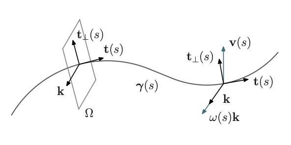
Figure 1: Sketch of a Timoshenko beam with local triad and kinematic parameters.

At each point of the axis is associated a cross-section modeled by a two-dimensional domain $\Omega$. Denoting by $\,(\bullet)^{\prime}\,$ the derivative with respect to $s$, the tangent unit vectors field is defined as

$$\textbf{t}:=\boldsymbol{\gamma}^{\prime}$$ (1)

By applying the orthogonal linear transformation  R , which performs the rotation by $\pi/2$ counterclockwise in the plane $\,\boldsymbol{\pi}\,$, the transversal unit vectors field is obtained as

$$\textbf{t}_{\bot}:=\textbf{R}\textbf{t}$$ (2)

Then, we introduce the uniform unit vectors field $\,\textbf{k}:=\textbf{t}\times\textbf{t}_{\bot}\,$.

Since the curve $\boldsymbol{\gamma}$ is assumed to be regular, the vector $\textbf{t}^{\prime}$ is defined at each abscissa $s$. Thus, introducing the scalar geometric curvature of the beam axis $\,c:=\|\textbf{t}^{\prime}\|\,$, the normal unit vector is defined by $\,\mathbf{n}:=\textbf{t}^{\prime}/c\,$. Vectors $\,\textbf{t}_{\bot}\,$ and $\,\mathbf{n}\,$ are related as (Romano, 2002) $\,\textbf{t}_{\bot}=(\textbf{t}_{\bot}\cdot\mathbf{n})\,\mathbf{n}\,$.

The kinematic hypothesis of the Timoshenko beam model is that cross-sections are hinged to the beam axis; thus, denoting by $\,V\,$ the linear space of translations, the velocity $\,\mathbf{v}:[0,\textrm{L}]\mapsto V\,$ of the beam axis and the angular velocity of cross sections $\,\omega:[0,\textrm{L}]\mapsto\Re\,$ are independent parameters describing the beam kinematics.

The tangent deformation field kinematically compatible with $\mathbf{w}=\{\mathbf{v},\>\omega\}$ is composed of axial strain, shear strain and flexural curvature scalar fields, i.e. $\{\varepsilon_{\mathbf{w}},\gamma_{\mathbf{w}},\chi_{\mathbf{w}}\}:[0,L]\mapsto\Re$.

$$\mathbf{D}_{\mathbf{w}}=\begin{vmatrix}\varepsilon_{\mathbf{w}}\\ \gamma_{\mathbf{w}}\\ \chi_{\mathbf{w}}\end{vmatrix}=\begin{vmatrix}\mathbf{v}^{\prime}\cdot\textbf{t}\\ (\mathbf{v}^{\prime}\cdot\textbf{t}_{\bot})-\omega\\ \omega^{\prime}\end{vmatrix}$$ (3)

By duality with the tangent deformation field $\mathbf{D}_{\mathbf{w}}$, the stress $\,\boldsymbol{\sigma}\,$ in a Timoshenko beam is composed of axial force, shear force and bending moment scalar fields, that is $\{N,T,M\}:[0,L]\mapsto\Re\,$.

$$\boldsymbol{\sigma}=\begin{vmatrix}N\\ T\\ M\end{vmatrix}$$ (4)

Equilibrium is expressed by the variational condition that the external virtual power of the force system l is equal to the internal virtual power of the stress $\,\boldsymbol{\sigma}\,$, for any virtual translation velocity and angular velocity, i.e. $\delta\mathbf{w}=\{\delta\mathbf{v},\>\delta\omega\}$, fulfilling homogeneous kinematic boundary conditions

$${\langle}\kern 1.00006pt\textbf{{l}},\delta\mathbf{w}\kern 1.00006pt{\rangle}=\int_{0}^{L}\boldsymbol{\sigma}(s)\cdot\mathbf{D}_{\delta\mathbf{w}}(s)\,ds$$ (5)

Integrating by parts Eq. (5) we get vector differential equation and boundary conditions ruling equilibrium between stress $\,\boldsymbol{\sigma}\,$ and external force system l which is composed of a distributed vector loading $\,\mathbf{p}:[0,L]\mapsto V\,$, distributed bending couples $\,m:[0,L]\mapsto\Re\,$, boundary concentrated forces $\,{\mathbf{F}}_{0}\in V\,$ and $\,{\mathbf{F}}_{L}\in V\,$ and boundary concentrated bending couples $\,\mathcal{M}_{0}\in\Re\,$ and $\,\mathcal{M}_{L}\in\Re\,$.

Then, projecting the vector differential equation of equilibrium along t and $\textbf{t}_{\bot}$ directions we get the following differential problem in $\,[0,\textrm{L}]\,$

$$\left\{\begin{aligned} &N^{\prime}-T\,\textbf{t}_{\bot}\cdot\textbf{t}^{\prime}=-\mathbf{p}\cdot\textbf{t}\,\\ &T^{\prime}-N\,\textbf{t}\cdot\textbf{t}_{\bot}^{\prime}=-\mathbf{p}\cdot\textbf{t}_{\bot}\,\\ &T+M^{\prime}=-m\end{aligned}\right.$$ (6)

equipped with the boundary conditions at $\,s=0\,$ and $\,s=L\,$

$$\left\{\begin{aligned} -(N\textbf{t}+T\textbf{t}_{\bot})(0)\cdot\delta\mathbf{v}(0)&={\mathbf{F}}_{0}(0)\cdot\delta\mathbf{v}(0)\,\\ (N\textbf{t}+T\textbf{t}_{\bot})(L)\cdot\delta\mathbf{v}(L)&={\mathbf{F}}_{0}(L)\cdot\delta\mathbf{v}(L)\,\\ -M(0)\;\delta\omega(0)&=\mathcal{M}_{0}\;\delta\omega(0)\,\\ M(L)\;\delta\omega(L)&=\mathcal{M}_{L}\;\delta\omega(L)\,\end{aligned}\right.$$ (7)

From Eqs. (7), natural static boundary conditions follow from essential kinematic boundary conditions related to the assigned constraints. When essential boundary conditions are not prescribed, i.e. virtual translation velocity $\,\delta\mathbf{v}\,$ and angular velocity $\,\delta\omega\,$ are arbitrary, the corresponding natural static conditions from Eqs. (7) are:

$$\left\{\begin{aligned} -(N\textbf{t}+T\textbf{t}_{\bot})(0)&={\mathbf{F}}_{0}(0)\,\\ (N\textbf{t}+T\textbf{t}_{\bot})(L)&={\mathbf{F}}_{0}(L)\,\\ -M(0)&=\mathcal{M}_{0}\,\\ M(L)&=\mathcal{M}_{L}\end{aligned}\right.$$ (8)

Explicit prescriptions of essential and natural boundary conditions for usual constraints adopted in structural mechanics are provided in the section named ”Case-studies”.

3 Stress-driven mixture model

In this section we will first recall the classical theory of local elasticity for a Timoshenko curved beam. Let us denote by $\,E\,$ and $\,G\,$ Euler-Young and shear moduli, respectively. $\,A\,$ stands for cross-sectional area and $\,J_{c}\,$ is the moment of inertia along the bending axis $\eta$ which is identified by the direction of the transversal unit vector $\,\textbf{t}_{\bot}\,$, that is:

$$J_{c}=\int_{\Omega}\eta^{2}\frac{1}{1-c\,\eta\>(\textbf{n}\cdot\textbf{t}_{\bot})}\,dA\,$$ (9)

The constitutive equations of local elasticity for curved beams are expressed following the treatments by Winkler (1858); Baldacci (1983), generalized by the presence of $\textbf{n}\cdot\textbf{t}_{\bot}$, that is

$$\left\{\begin{aligned} \varepsilon_{l}(s)&=\frac{1}{EA}\biggr{[}N+\frac{\textit{c}\,M}{\textbf{n}\cdot\textbf{t}_{\bot}}\biggr{]}(s)\,\\ \chi_{l}(s)&=\frac{M}{EJ_{c}}(s)+(\textbf{n}\cdot\textbf{t}_{\bot})\frac{\textit{c}}{EA}\biggr{[}N+\frac{\textit{c}\,M}{\textbf{n}\cdot\textbf{t}_{\bot}}\biggr{]}(s)\,\\ \gamma_{l}(s)&=\bigg{[}\frac{T}{GK_{r}}\bigg{]}(s)\end{aligned}\right.$$ (10)

where the equilibrium differential equation $T+M^{\prime}=-m$ has been considered in Eq. (10)₃, assuming vanishing distributed bending couples.

$K_{r}$ in Eq. (10)₃ is the shear stiffness for a curved beam defined as follows

$$K_{r}^{-1}=\int_{\Omega}\frac{r^{2}}{{[r-\eta(\textbf{n}\cdot\textbf{t}_{\bot})]}^{2}\>b^{2}}\bigg{[}\frac{S_{c}}{J_{c}}-\frac{A^{*}}{(\textbf{n}\cdot\textbf{t}_{\bot})rA}\bigg{]}^{2}\,dA$$ (11)

where $r=1/c$ is the curvature radius and $S_{c}$ is the static moment of $A^{*}$, that is

$$S_{c}:=\int_{\Omega^{*}}\frac{\eta}{1-c\,\eta\>(\textbf{n}\cdot\textbf{t}_{\bot})}\,dA^{*}$$ (12)

For a Timoshenko curved nanobeam the nonlocal elastic deformation fields are expressed by the stress-driven mixture model consisting in a convex combination of the local response in Eq. (10) and a nonlocal response obtained by a convolution between the local field and a scalar averaging kernel $\,\phi:\Re\mapsto[0;+\infty[$.

Let preliminarily inticate with i and f the vectors collecting source and output fields, i.e.: $\textbf{i}=\{\varepsilon_{l},\chi_{l},\gamma_{l}\};\>\textbf{f}=\{\varepsilon,\chi,\gamma\}$. Then, by denoting with $0\leq m\leq 1$ the mixture parameter and with $l_{c}$ a positive nonlocal length parameter, the stress-driven mixture model is expressed as follows

$$\textbf{f}(s)=m\>\textbf{i}(s)+(1-m)\>\int_{0}^{L}{\phi_{\l_{c}}(s,\xi)\>\textbf{i}(\xi)\>d\xi}$$ (13)

which is a Fredholm integral equation of the second kind in the unknown source field i.

The averaging kernel is assumed to be the special bi-exponential function adopted by Eringen (1983), that is

$$\phi_{\l_{c}}(s)=\frac{1}{2\l_{c}}\exp(-\frac{|s|}{\l_{c}})\,$$ (14)

By extending to Timoshenko curved beams the Mixture equivalence by Romano et al. (2017b, Lemma 2), it can be proved that the integral convolutions in Eq. (13) is equivalent to the following differential equation

$$\frac{\textbf{f}(s)}{\l_{c}^{2}}-\,\partial_{s}^{2}\textbf{f}(s)=\frac{\textbf{i}(s)}{\l_{c}^{2}}-m\>\partial_{s}^{2}\textbf{i}(s)$$ (15)

equipped with the constitutive boundary conditions

$$\left\{\begin{aligned} &\partial_{s}\textbf{f}(0)=\frac{1}{\l_{c}}\,\textbf{f}(0)+m\>\bigg{(}\partial_{s}\textbf{i}(0)-\frac{\textbf{i}(0)}{\l_{c}}\bigg{)}\,\\ &\partial_{s}\textbf{f}(L)=-\frac{1}{\l_{c}}\,\textbf{f}(L)+m\>\bigg{(}\partial_{s}\textbf{i}(L)+\frac{\textbf{i}(L)}{\l_{c}}\bigg{)}\end{aligned}\right.$$ (16)

The stress-driven mixture model in Eq. (13) is purely nonlocal when $m=0$ and purely local when $m=1$. Since the model is based on two parameters (i.e. mixture and nonlocal length parameters) it is able to provide softening or stiffening responses as shown in the section ”Case-studies” and therefore can effectively model a wide range of nano-engineering problems.

4 Elastic equilibrium of Timoshenko curved nanobeams

Let us consider the linearized, plane and curved Timoshenko beam model and denote by $\,\textbf{u}:[0,\textrm{L}]\mapsto V\,$ the displacement vector field of the structural axis and by $\,\varphi:[0,\textrm{L}]\mapsto\Re\,$ the scalar field of rotations of cross-sections.

From Eq. (3), the kinematically compatible deformation field $\,\mathbf{D}_{\textbf{w}}\,$ associated with $\textbf{w}=\{\textbf{u},\varphi\}$ is composed of axial strain $\varepsilon_{\textbf{w}}:[0,L]\mapsto\Re$, shear strain $\gamma_{\textbf{w}}:[0,L]\mapsto\Re$ and flexural curvature $\chi_{\textbf{w}}:[0,L]\mapsto\Re$ scalar fields.

$$\mathbf{D}_{\textbf{w}}=\begin{vmatrix}\varepsilon_{\textbf{w}}\\ \gamma_{\textbf{w}}\\ \chi_{\textbf{w}}\end{vmatrix}=\begin{vmatrix}\textbf{u}^{\prime}\cdot\textbf{t}\\ (\textbf{u}^{\prime}\cdot\textbf{t}_{\bot})-\varphi\\ \varphi^{\prime}\end{vmatrix}$$ (17)

Hence, by virtue of Eq. (17)₃, the scalar field of rotations is expressed by the following integration formula

$$\varphi(s)=\varphi(0)+\int_{0}^{s}\chi_{\textbf{w}}(\xi)\,d\xi\,$$ (18)

Let us consider the subsequent additive decomposition where Eq. (17)${}_{1,2}\,$ is taken into account

$$\textbf{u}^{\prime}=(\textbf{u}^{\prime}\cdot\textbf{t})\,\textbf{t}+(\textbf{u}^{\prime}\cdot\textbf{t}_{\bot})\,\textbf{t}_{\bot}=\varepsilon_{\textbf{w}}\,\textbf{t}+(\gamma_{\textbf{w}}+\varphi)\,\textbf{t}_{\bot}\,$$ (19)

with $\,\varphi\,$ given by Eq. (18).

By integrating the previous equation, the displacements field  u  can be expressed as follows

$$\begin{split}\textbf{u}(s)&=\textbf{u}(0)+\int_{0}^{s}\textbf{u}^{\prime}d\xi\,\\ &=\textbf{u}(0)+\int_{0}^{s}[\varepsilon_{\textbf{w}}(\xi)\,\textbf{t}(\xi)+(\gamma_{\textbf{w}}(\xi)+\varphi(\xi))\,\textbf{t}_{\bot}(\xi)]\,d\xi\,\end{split}$$ (20)

Thus, the local-nonlocal mixture elastostatic problem of a Timoshenko curved beam is composed of the differential equilibrium equations (6) equipped with the boundary conditions (7), the constitutive equations provided by the integral convolutions in Eq. (13) (or by the equivalent differential problem in Eqs. (15)-(16)) and the kinematic compatibility condition expressed by Eqs. (18) and (20). The integration constants $\,\varphi(0)\in\Re\,$ and $\,\textbf{u}(0)\in V\,$ are univocally evaluated by prescribing essential kinematic boundary conditions.

5 Case-studies

The procedure to solve the elastostatic problem of a Timoshenko nonlocal curved beam is now illustrated with reference to some cases of applicative interest in Nanotechnology.

A silicon carbide nanobeam, with Euler-Young modulus $E=427\>$ [GPa] and Poisson ratio $\nu=0.2$ is considered. The beam axis is assumed to be a circle arc of radius $r=10\>$ [nm] so that the beam length is $L=r\,\pi/2$. The cross-section is a rectangular domain $\Omega$ of base $b=5~{}$[nm] and height $h=2L/3$. In the present section, the following non-dimensional nonlocal parameter is adopted

$$\lambda=\frac{l_{c}}{L}$$ (21)

where $l_{c}$ is the nonlocal characteristic length parameter.

A simple procedure is proposed in order to solve the elastostatic problem of the curved nanobeam introduced above and to investigate size-dependent responses. It consists of the following steps.

• Step 1. Solution of the differential equilibrium problem in Eqs. (6)-(7) to obtain the stress fields composed of axial force $N$, shear force $T$ and bending moment $M$ as functions of $n$ integration constants, with $n$ standing for redundancy degree. For statically determinate beams for which $n=0$, the stress fields are univocally determined by equilibrium requirements.

• Step 2. Evaluation of nonlocal strain fields by applying the nonlocal stress-driven mixture model in Eq. (13) or by solving the equivalent differential problem governed by Eqs. (15)-(16).

• Step 3. Detection of curved nanobeam nonlocal displacements u and rotations $\varphi$ fields by imposing $3+n$ essential kinematic boundary conditions.

Note that in the case-studies presented in this section, total deformations and elastic deformation fields are assumed to be coincident.

Cantilever beam under point-force at free end

The curved nanobeam introduced above is clamped at the abscissa $\,s=0\,$ and subjected to a force $\,F=10\,$ [nN] applied at free end, as shown in Fig. 2. Hence, the essential kinematic boundary conditions are

$$\textbf{u}(0)=\mathbf{o}\,\qquad\varphi(0)=0\,$$ (22)

From Eqs. (7) and (22) follows that natural static boundary conditions are expressed by

$$\begin{cases}N(L)&=0\\ T(L)&=F\\ M(L)&=0\end{cases}$$ (23)

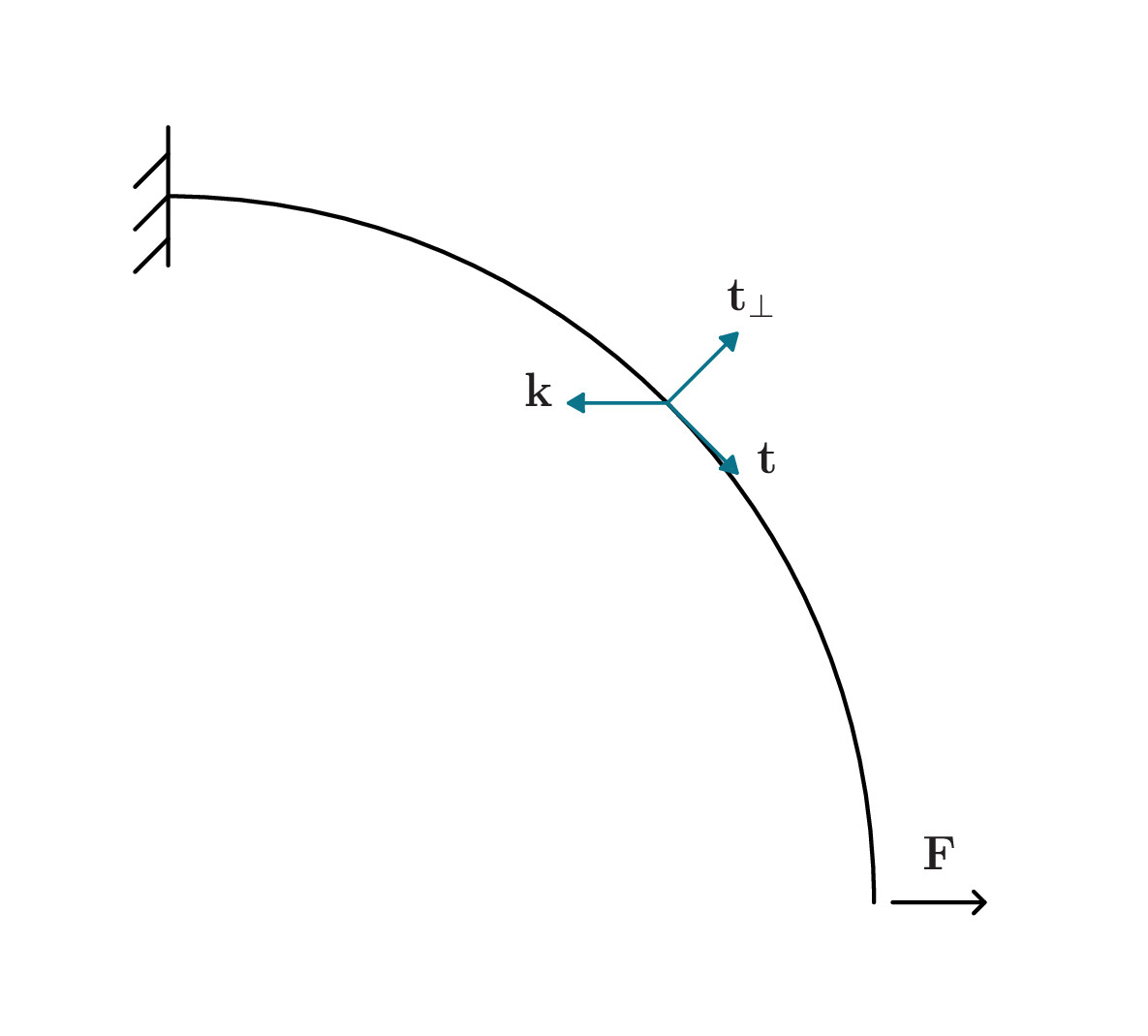
Figure 2: Cantilever curved nanobeam.

Since the redundancy degree $\,n\,$ is vanishing, by following $Step~{}1$ the stress fields of axial force $N$, shear force $T$ and bending moment $M$ are univocally determined by equilibrium requirements in Eqs. (6)-(7) and their parametric expressions are provided below:

$$\begin{cases}&N(s)=F\,\cos\big{(}s/r\big{)}\\ &T(s)=F\,\sin\big{(}s/r\big{)}\\ &M(s)=F\,r\cos\big{(}s/r\big{)}\end{cases}$$ (24)

Transversal displacements $u_{t_{\bot}}=\textbf{u}\cdot\textbf{t}_{\bot}$, axial displacements $u_{t}=\textbf{u}\cdot\textbf{t}$ and bending rotations $\varphi$ are obtained by following $Steps~{}2$-$\,3$ and then plotted as fuction of $s\in[0,L]$ as shown in Figs. 6 - 8. In particular Figs. 6 - 8 represent displacements and rotations of the nanocantilever for increasing values of the nonlocal parameter $\lambda$, for fixed values of the mixture parameter. As also shown by numerical results in Tab. 1, the response stiffens for increasing values of the nonlocal parameter $\lambda$ and exhibits a softening behavior by increasing the mixture parameter $m$.

Slider and roller supported beam under uniformly distributed loading

The curved nanobeam has a slider and a roller supports, at $s=0$ and $s=L$ respectively. It is subjected to a uniformly distributed vertical loading $\,q=2\,$ [nN/nm] directed upwards as shown in Fig. 3. Now, the essential kinematic boundary conditions are

$$\textbf{u}(0)\cdot\textbf{t}(0)=0\,\qquad\varphi(0)=0\,\qquad\textbf{u}(L)\cdot\textbf{t}(L)=0\,$$ (25)

From Eqs. (7) and (22) follows that natural static boundary conditions are expressed by

$$\left\{\begin{split}T(0)&=0\,\\ T(L)&=0\,\\ M(L)&=0\,\end{split}\right.$$ (26)

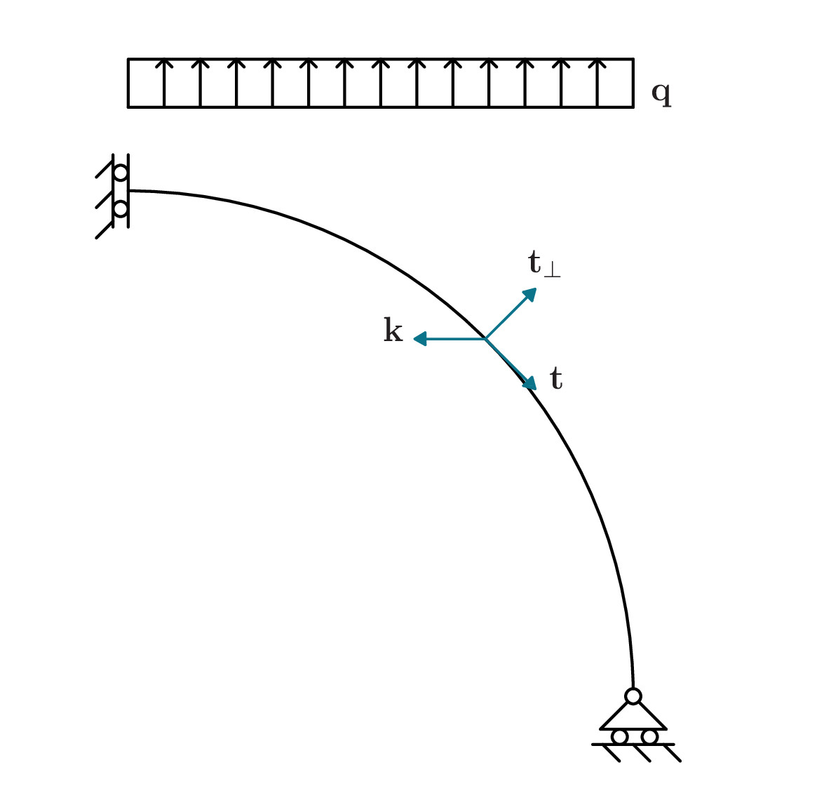
Figure 3: Curved nanobeam with slider and roller supports.

Since the beam is statically determinate, the stress fields $\,N\,,T\,,M\,$ are univocally obtained by equilibrium conditions and their parametric expressions as function of the arch length are shown as follows:

$$\begin{cases}&N(s)=q\,r\sin^{2}\big{(}s/r\big{)}\\ &T(s)=-\frac{1}{2}q\,r\sin\big{(}2s/r\big{)}\\ &M(s)=-\frac{1}{2}q\,r^{2}\cos^{2}\big{(}s/r\big{)}\end{cases}$$ (27)

Then, the transversal displacements $u_{t_{\bot}}=\textbf{u}\cdot\textbf{t}_{\bot}$, axial displacements $u_{t}=\textbf{u}\cdot\textbf{t}$ and bending rotations $\varphi$ are obtained by following $Steps~{}2$-$\,3$ and represented in Figs. 9 - 11 as function of $\lambda$ for fixed values of the mixture parameters $m$. Numerical results in terms of displacements and rotations are provided in Tab. 2.

Clamped and roller supported beam under uniformly distributed loading

Let us consider a curved nanobeam with clamped and roller supported ends, at $s=0$ and $s=L$ respectively. It is subjected to a uniformly distributed vertical loading $\,q=5\,$ [nN/nm] directed upwards as shown in Fig. 4. Hence, the essential kinematic boundary conditions are

$$\textbf{u}(0)=0\,\qquad\varphi(0)=0\,\qquad\textbf{u}(L)\cdot\textbf{t}(L)=0\,$$ (28)

From Eqs. (7) and (28) the corrisponding natural static boundary conditions take the form

$$\left\{\begin{split}T(L)&=0\,\\ M(L)&=0\,\end{split}\right.$$ (29)

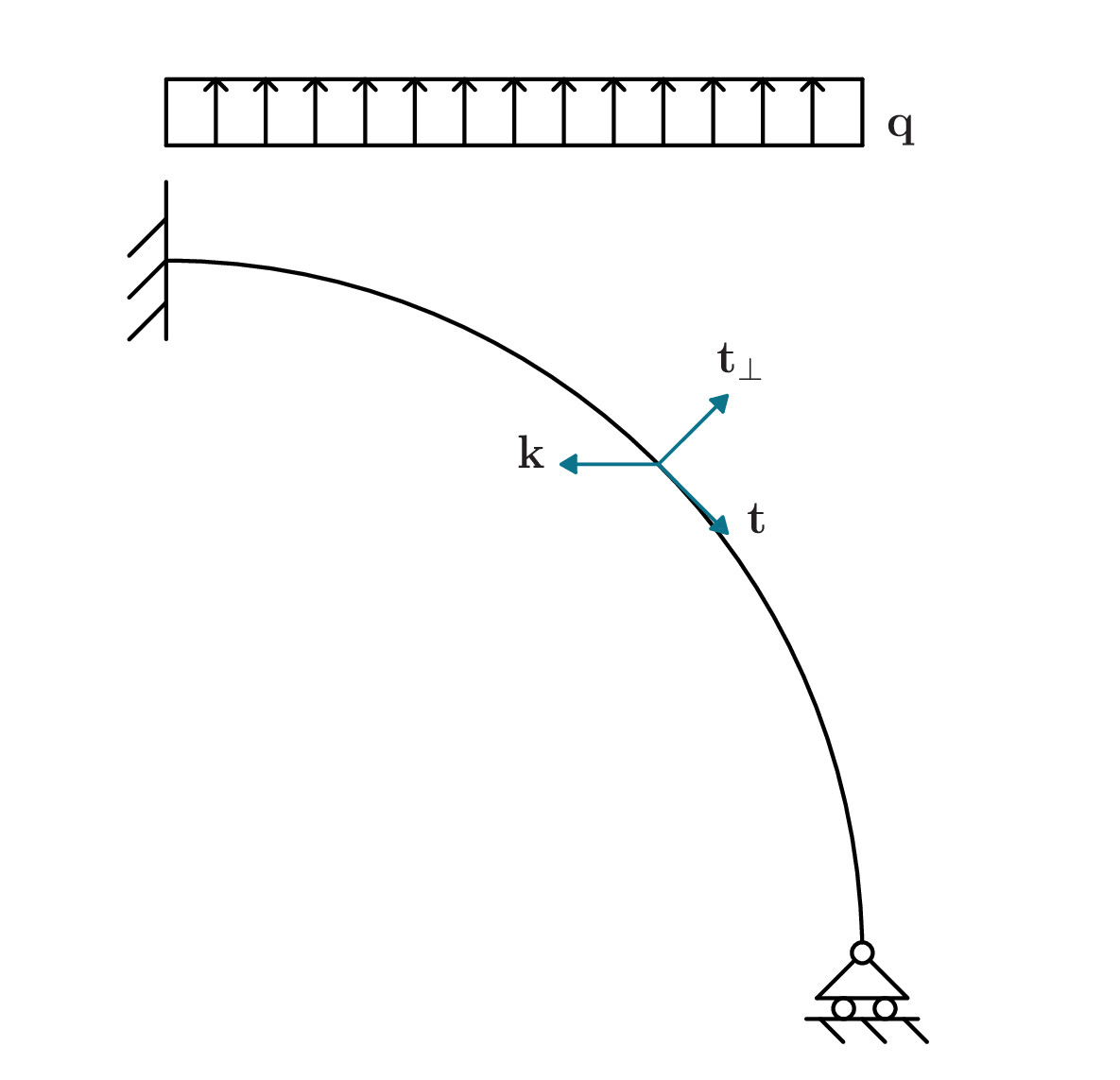
Figure 4: Clamped and roller supported curved nanobeam.

Axial force $N$, shear force $T$ and bending moment $M$ are solutions of the differential equilibrium problem in Eqs. (6)-(29) and since the redundancy degree is $n=1$, the stress fields are functions of one integration costant. Parametric nonlocal strain fields are obtained by the integral stress-driven mixture model in Eq. (13) or by solving the equivalent differential problem in Eqs. (15)-(16). Then, nonlocal displacements u and rotations $\varphi$ are detected by imposing the $3+n$ essential kinematic boundary conditions in Eq. (28). The static fields of axial force $\,\textbf{R}N\textbf{t}=N\textbf{t}_{\bot}\,$, shear force $\,T\textbf{t}_{\bot}\,$ and bending moment $\,\textbf{R}M\textbf{k}=-M\textbf{t}_{\bot}\,$, parameterized in terms of the arch length $s$, are graphically represented in Figs. 12, 13, 14, respectively. A schematic sketch of cross section with the local triad and the vectors $\textbf{R}M\textbf{k}\,$ and $\textbf{R}N\textbf{t}$ is depicted in Fig. 5.

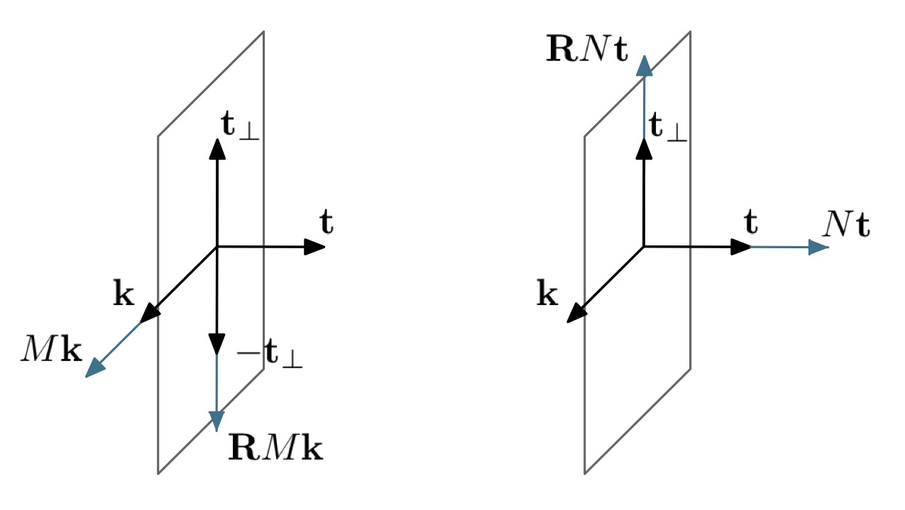
Figure 5: Sketch of cross section with local triad and bending $\textbf{R}M\textbf{k}\,$ and axial $\textbf{R}N\textbf{t}$ vectors.

Transversal displacements $u_{t_{\bot}}=\textbf{u}\cdot\textbf{t}_{\bot}$, axial displacements $u_{t}=\textbf{u}\cdot\textbf{t}$ and bending rotations $\varphi$ are plotted versus $s\in[0,L]$ in Figs. 15 - 17. As it is shown in the parametric plots, the response stiffens for increasing nonlocal parameter $\lambda$ and exhibits a softening behavior by increasing the mixture parameter $m$. This trend is also confirmed by numerical results provided in Tab. 3.

Remark. It is worth noting that for vanishing geometric curvature and mixture parameters, solution procedures and results of the case-studies illustrated in this section are coincident with the ones provided by Barretta et. al(B, 2018) for straight Timoshenko nanobeams. An alternative solution methodolody for straight thick nonlocal beams based on Laplace trasform has been recently proposed by Zhang et al.(ZhangJ, 2019).

(a)

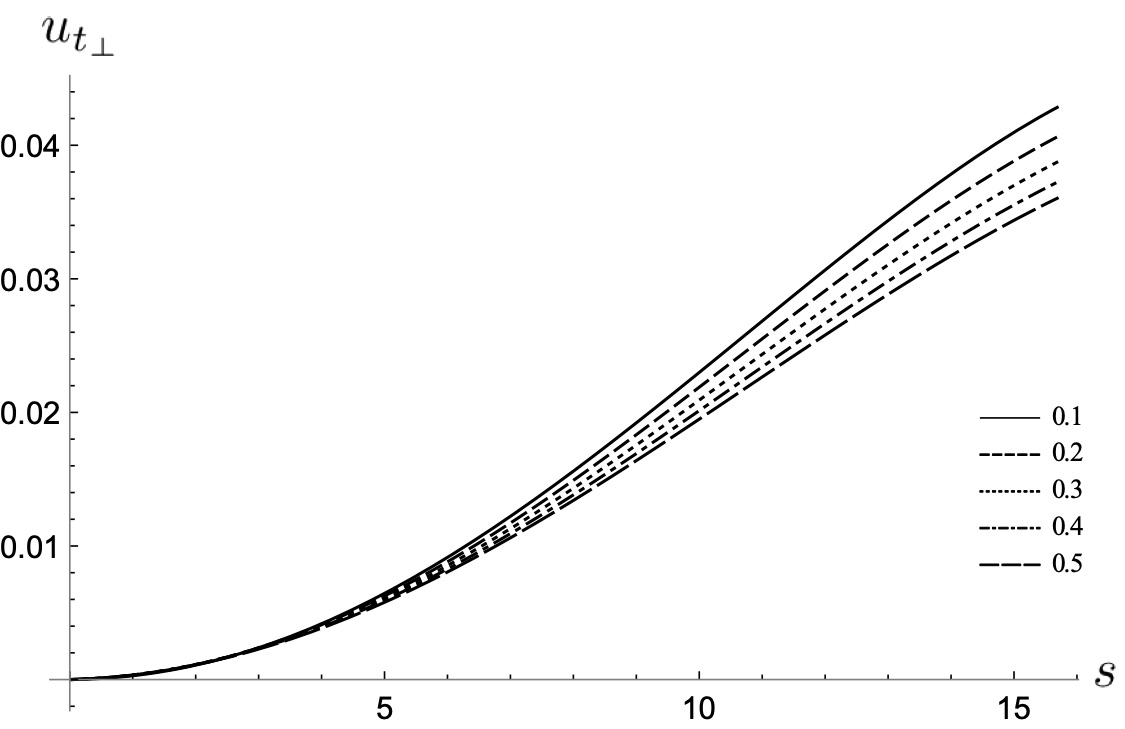
(b)

Figure 6: Cantilever beam: nonlocal transversal displacement $u_{\textbf{t}_{\bot}}$ [nm] versus $s\in[0,L]$ [nm] as fuction of $\lambda$.

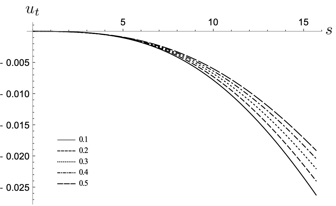
(a)

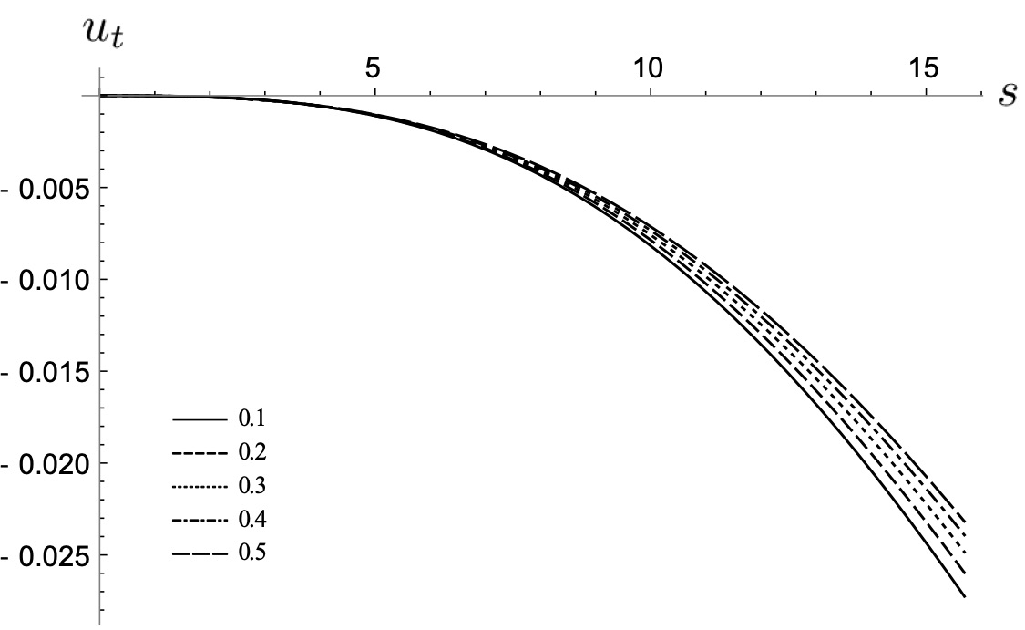
(b)

Figure 7: Cantilever beam: nonlocal axial displacement $u_{\textbf{t}}$ [nm] versus $s\in[0,L]$ [nm] as fuction of $\lambda$.

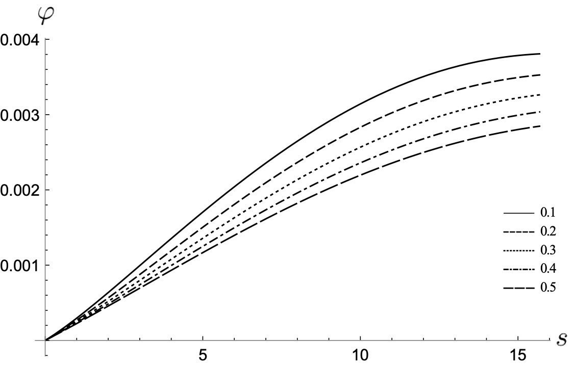
(a)

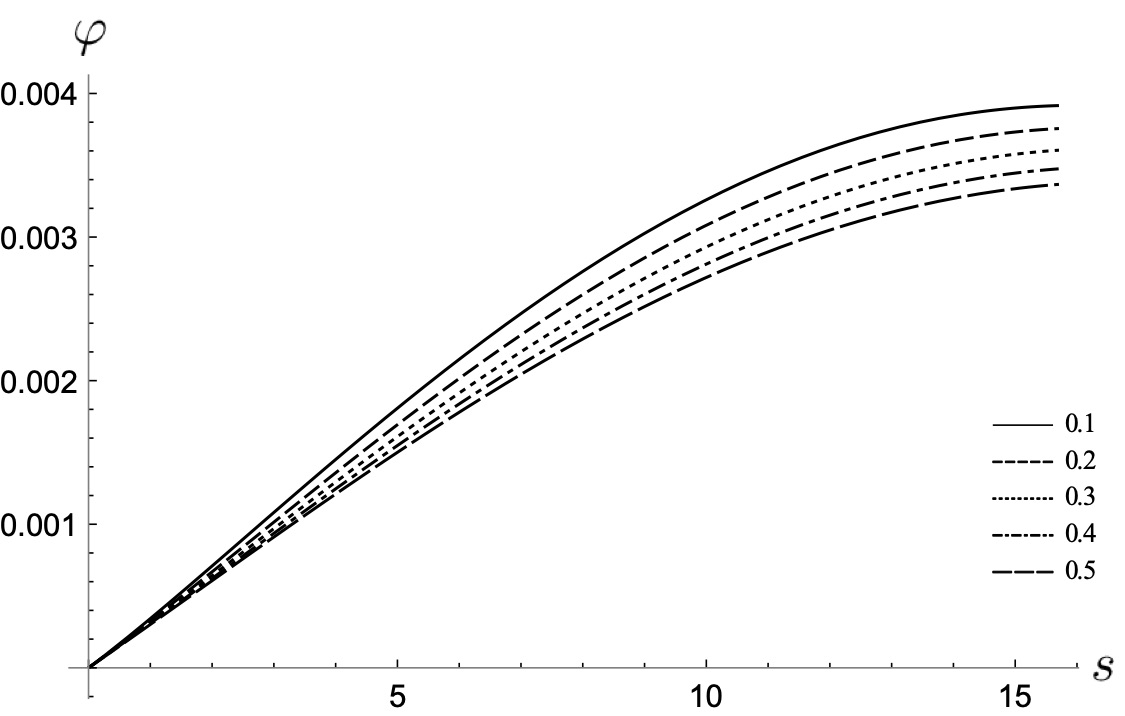
(b)

Figure 8: Cantilever beam: nonlocal bending rotation $\varphi$ [-] versus $s\in[0,L]$ [nm] as fuction of $\lambda$.

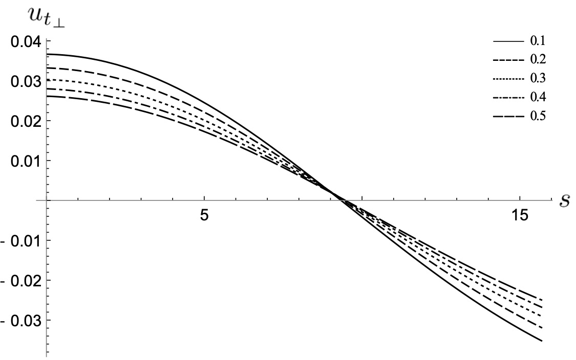
(a)

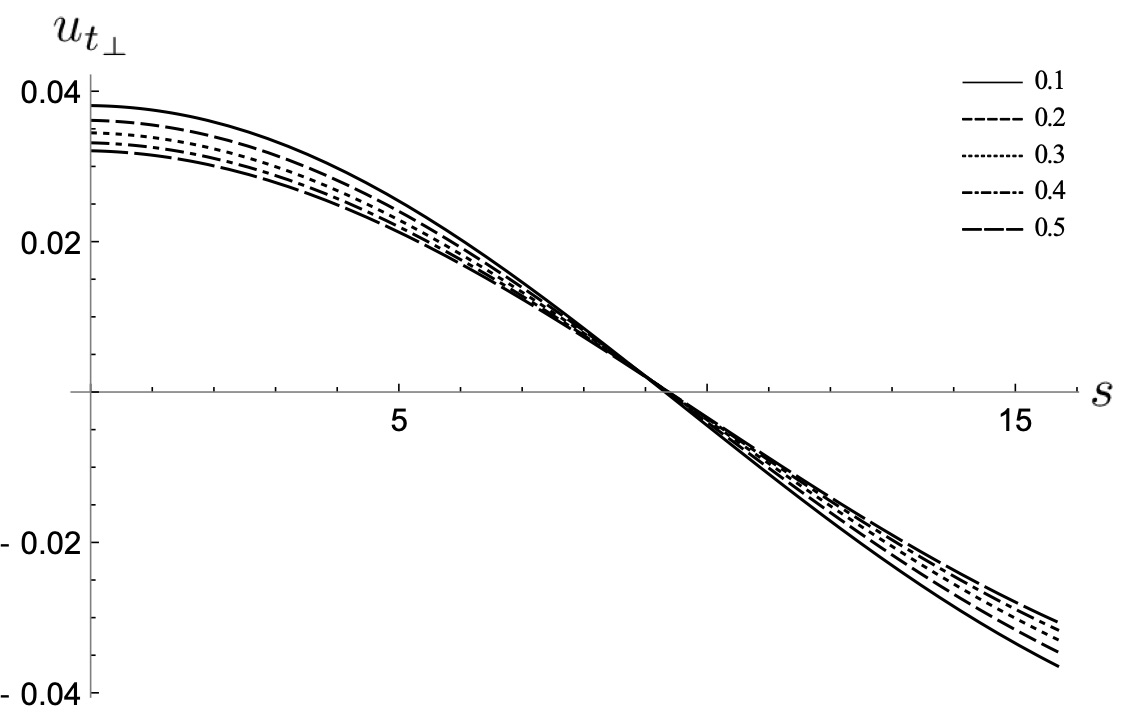
(b)

Figure 9: Slider and roller supported beam: nonlocal transversal displacement $u_{\textbf{t}_{\bot}}$ [nm] versus $s\in[0,L]$ [nm] as fuction of $\lambda$.

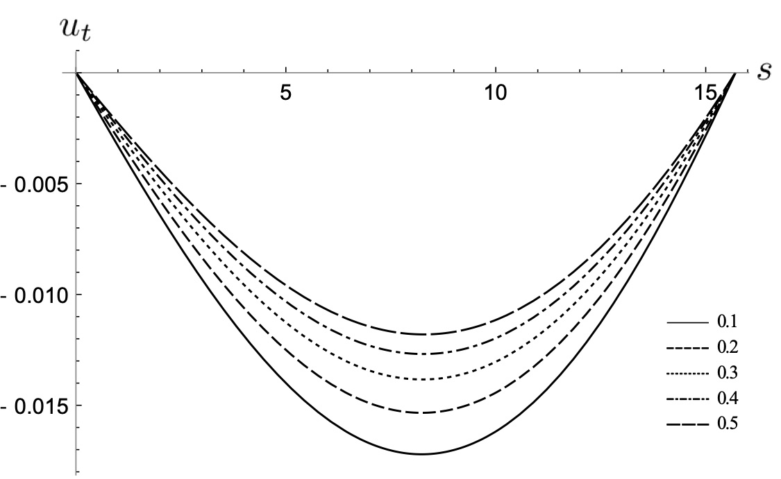
(a)

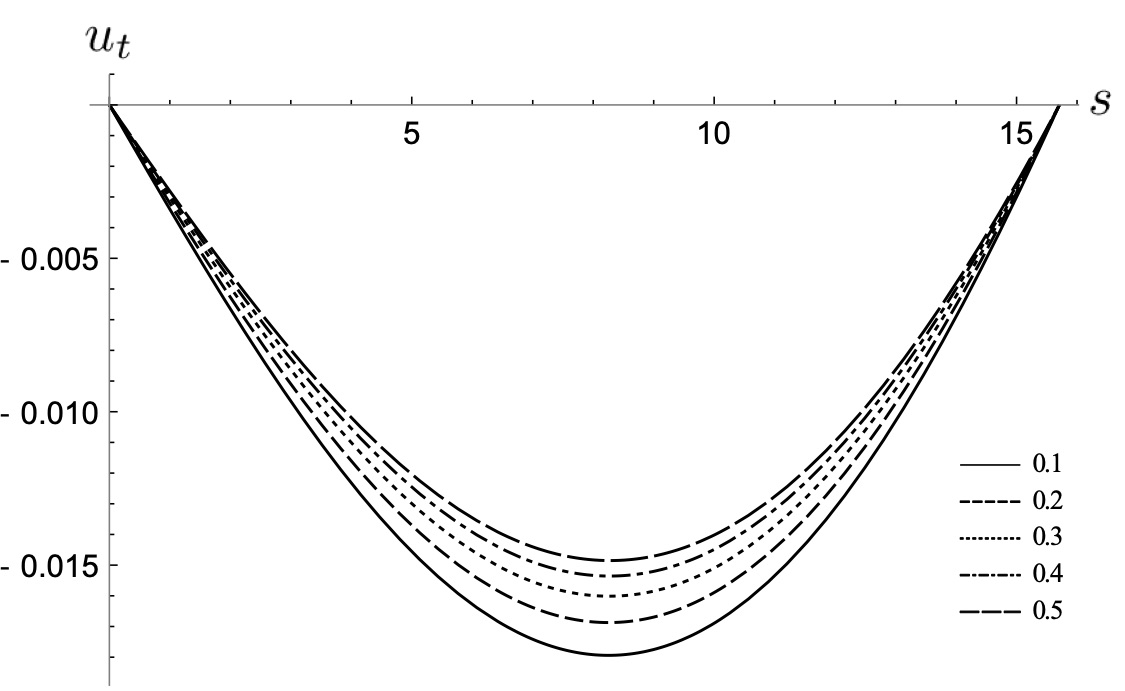
(b)

Figure 10: Slider and roller supported beam: nonlocal axial displacement $u_{\textbf{t}}$ [nm] versus $s\in[0,L]$ [nm] as fuction of $\lambda$.

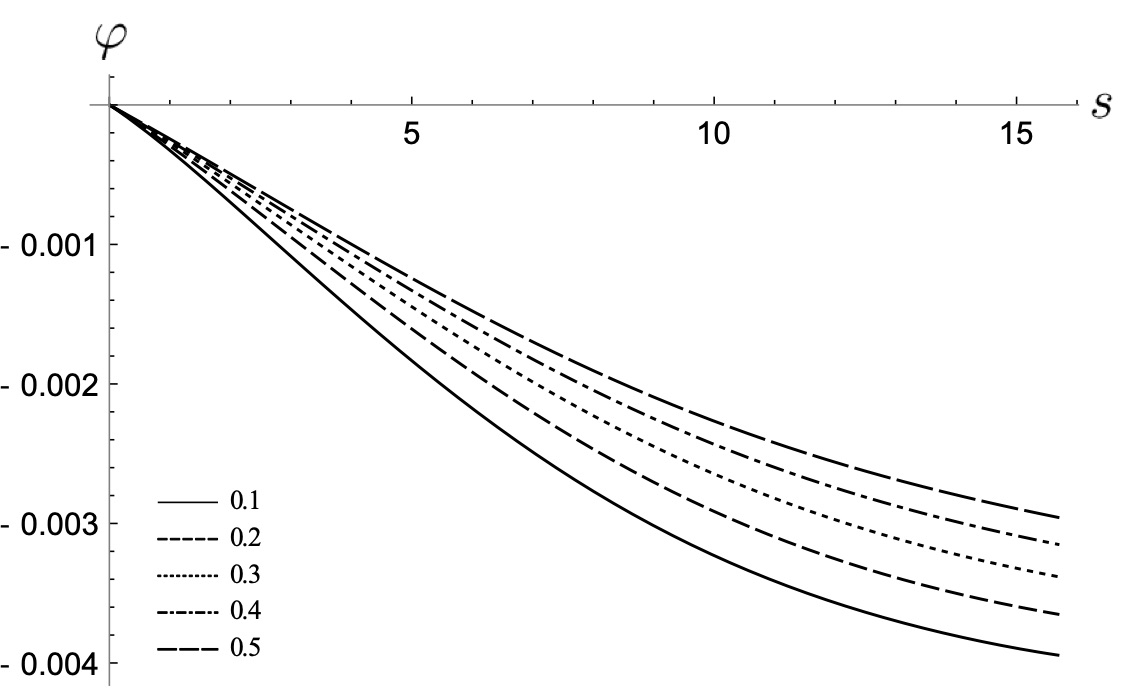
(a)

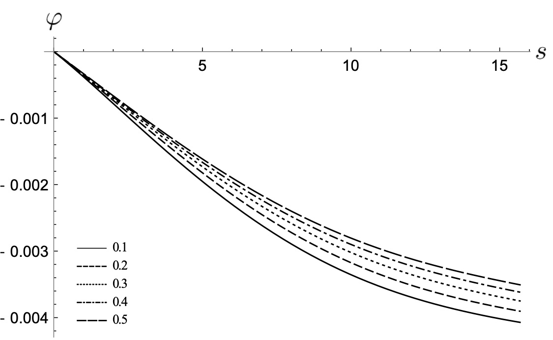
(b)

Figure 11: Slider and roller supported beam: nonlocal bending rotation $\varphi$ [-] versus $s\in[0,L]$ [nm] as fuction of $\lambda$.

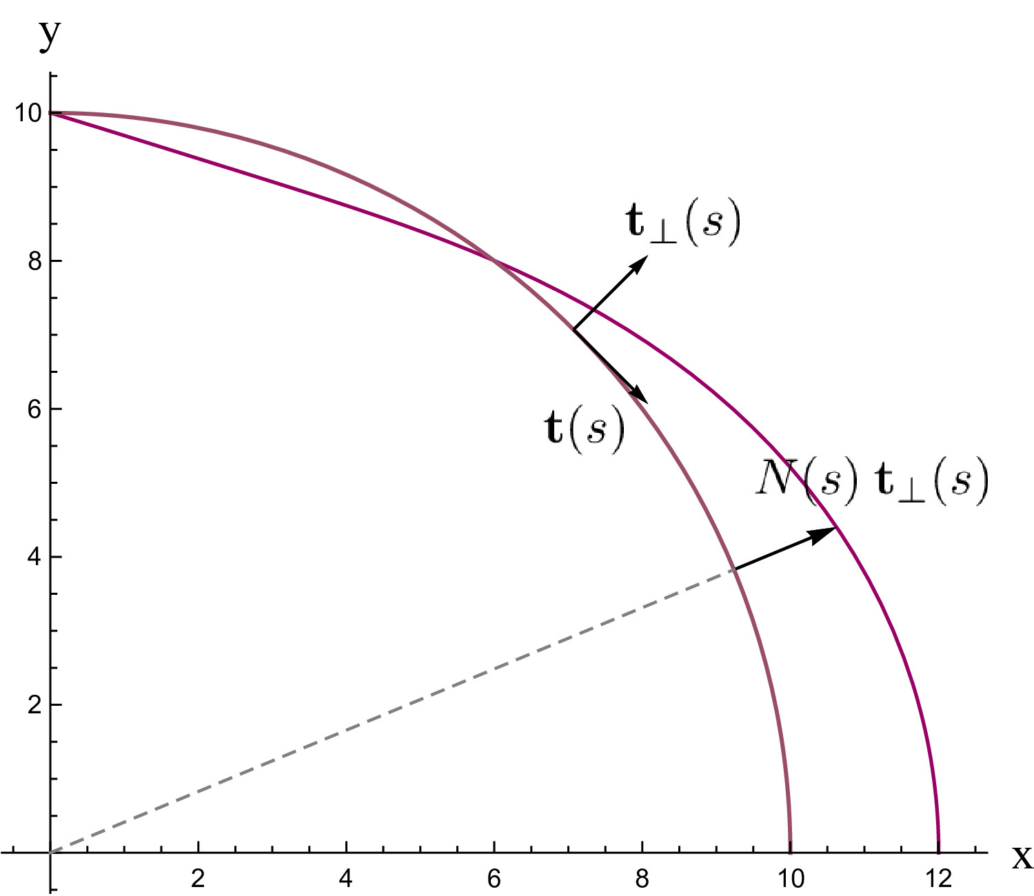
Figure 12: Clamped and roller supported beam: plot of the vector field $\textbf{R}N\textbf{t}=N\textbf{t}_{\bot}$ [10 nN] in the Cartesian plane x [nm], y [nm] for $\lambda=0.5$ and $m=0.3$.

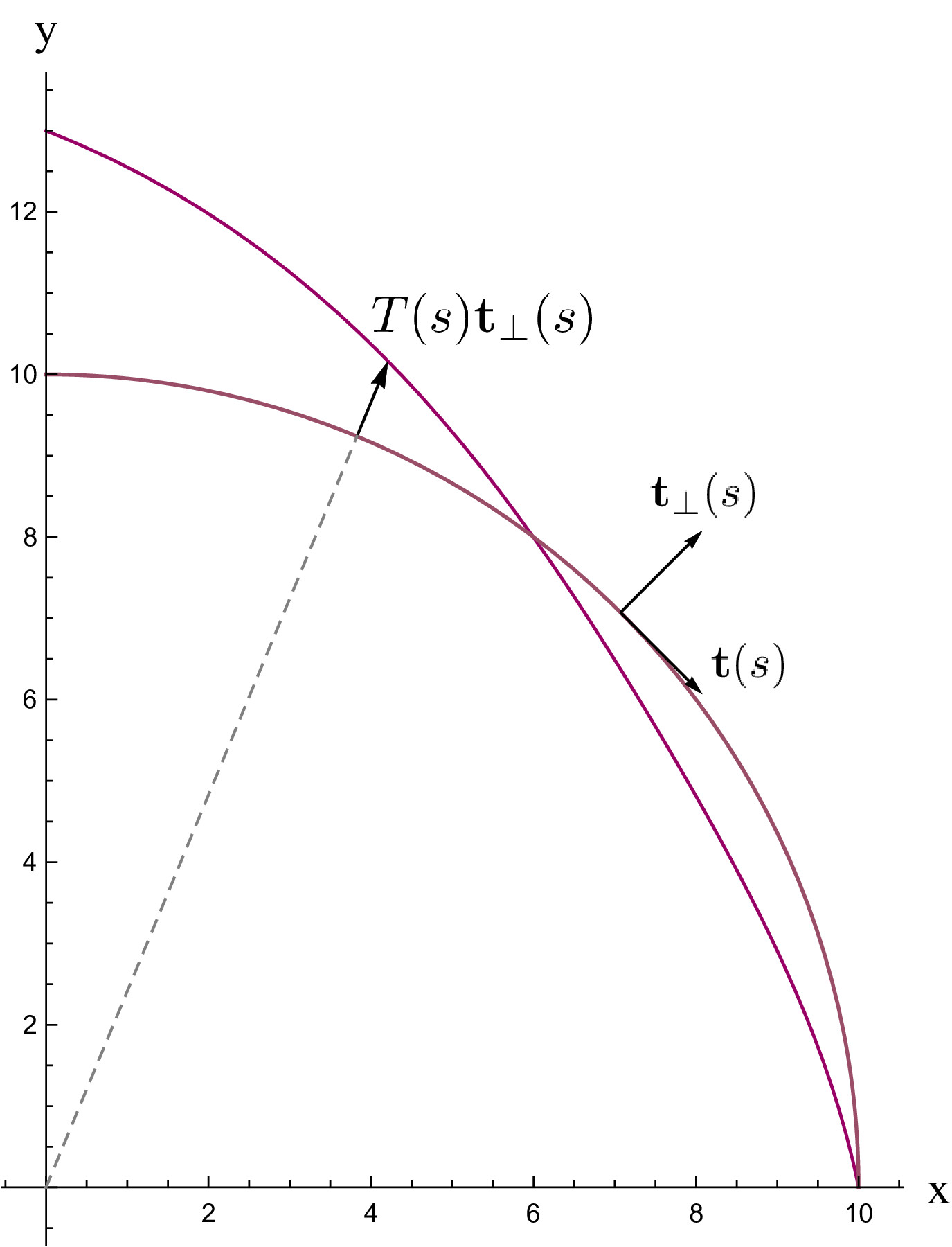
Figure 13: Clamped and roller supported beam: plot of the vector field $T\textbf{t}_{\bot}$ [10 nN] in the Cartesian plane x [nm], y [nm] for $\lambda=0.5$ and $m=0.3$.

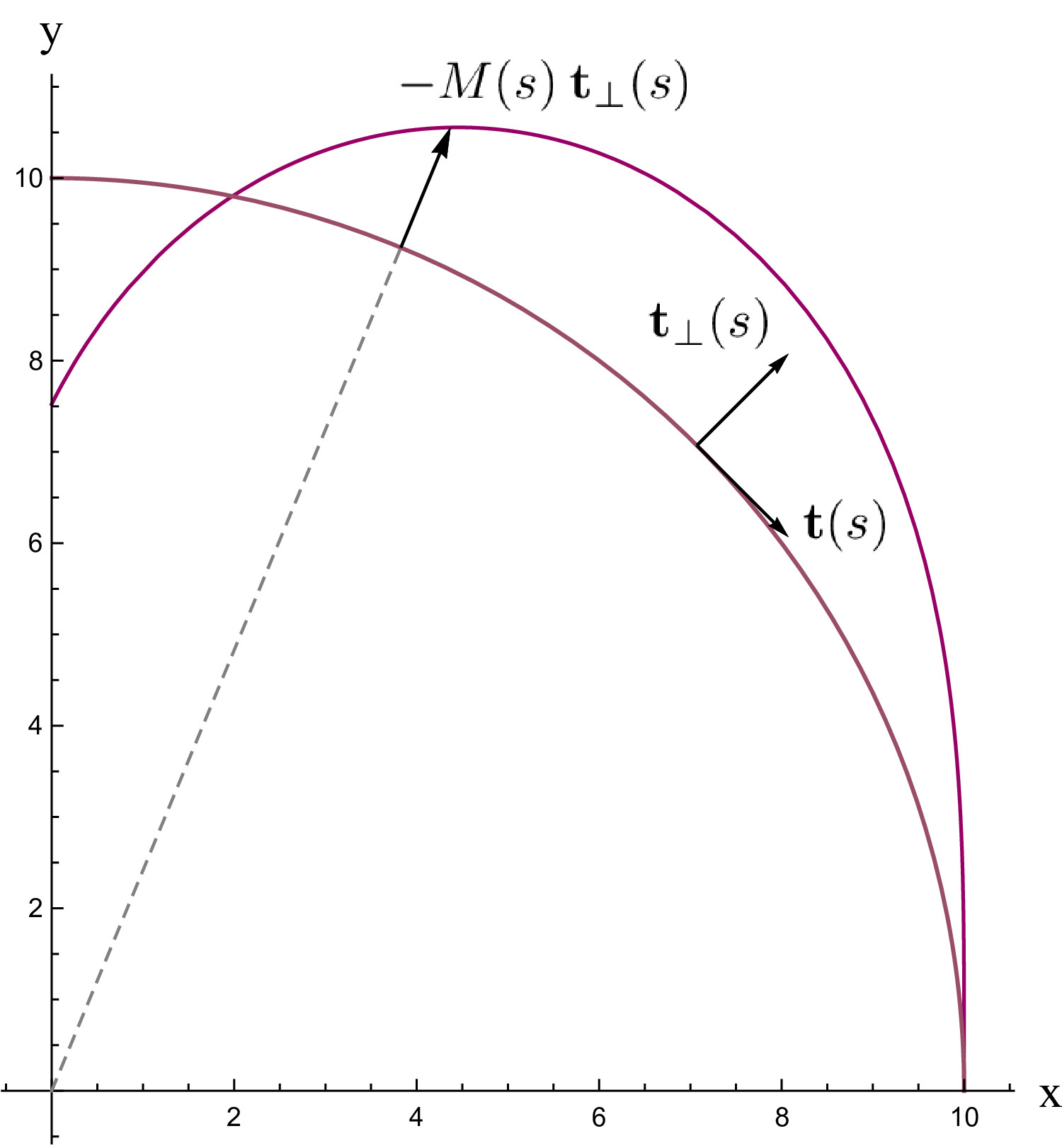
Figure 14: Clamped and roller supported beam: plot of the vector field $\textbf{R}M\textbf{k}=-M\textbf{t}_{\bot}$ [20 nN nm] in the Cartesian plane x [nm], y [nm] for $\lambda=0.5$ and $m=0.3$.

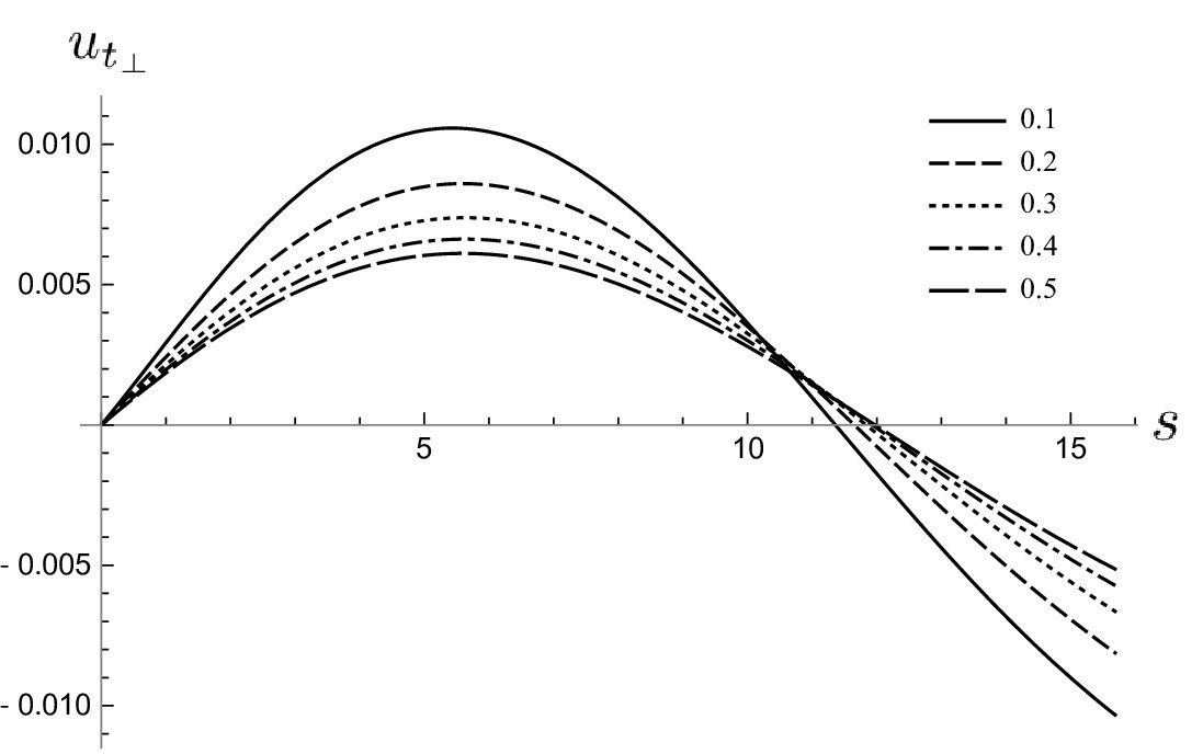
(a)

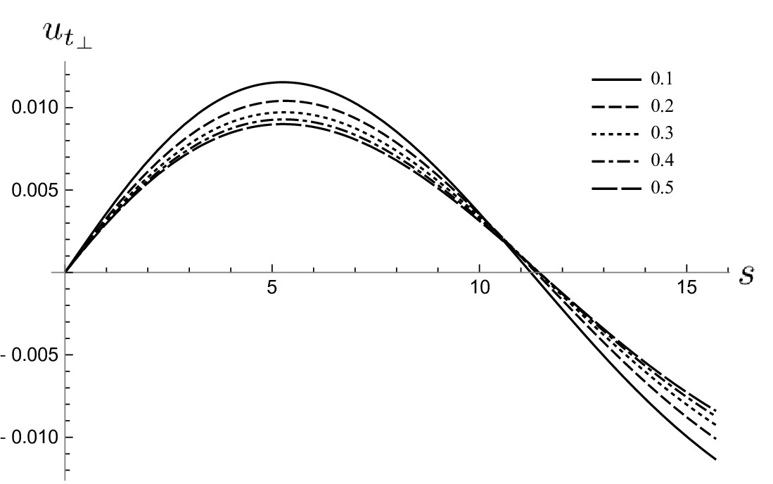
(b)

Figure 15: Clamped and roller supported beam: nonlocal transversal displacement $u_{\textbf{t}_{\bot}}$ [nm] versus $s\in[0,L]$ [nm] as fuction of $\lambda$.

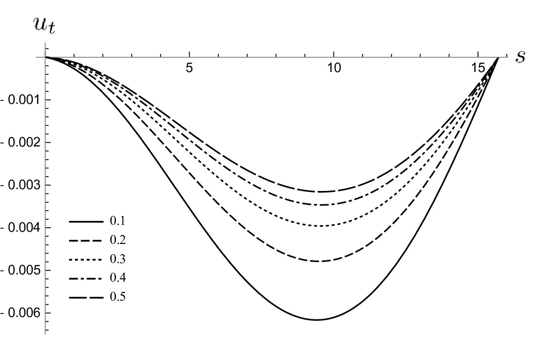
(a)

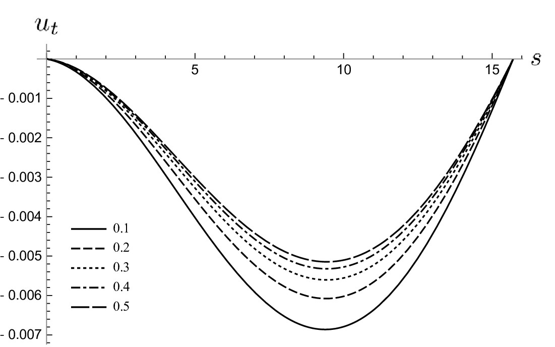
(b)

Figure 16: Clamped and roller supported beam: nonlocal axial displacement $u_{\textbf{t}}$ [nm] versus $s\in[0,L]$ [nm] as fuction of $\lambda$.

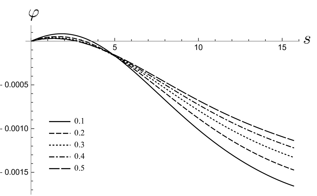
(a)

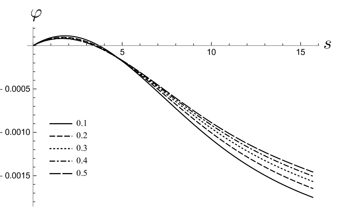
(b)

Figure 17: Clamped and roller supported beam: nonlocal bending rotation $\varphi$ [-] versus $s\in[0,L]$ [nm] as fuction of $\lambda$.

$\lambda$	$u_{\bot}(L)\>[10^{-2}nm]$		$u_{t}(L)\>[10^{-2}nm]$		$\varphi(L)\>[10^{-3}]$		$u^{tot}_{max}(L)\>[10^{-2}nm]$
	$m=0.3$	$m=0.6$	$m=0.3$	$m=0.6$	$m=0.3$	$m=0.6$	$m=0.3$	$m=0.6$
0,1	4,131	4,289	-2,633	-2,732	3,808	3,916	4,899	5,085
0,2	3,744	4,068	-2,406	-2,602	3,528	3,756	4,450	4,829
0,3	3,414	3,879	-2,209	-2,490	3,264	3,605	4,066	4,609
0,4	3,149	3,728	-2,048	-2,398	3,037	3,475	3,756	4,432
0,5	2,939	3,608	-1,916	-2,323	2,847	3,367	3,509	4,291
0,6	2,770	3,511	-1,809	-2,261	2,690	3,277	3,308	4,176
0,7	2,632	3,432	-1,721	-2,211	2,558	3,202	3,145	4,083
0,8	2,518	3,367	-1,647	-2,169	2,447	3,138	3,008	4,005
0,9	2,422	3,312	-1,584	-2,133	2,352	3,084	2,894	3,939

Table 1: Cantilever beam: numerical outcomes.

$\lambda$	$u_{\bot}(0)\>[10^{-2}nm]$		$u_{\bot}(L)\>[10^{-2}nm]$		$\varphi(L)\>[10^{-3}]$		$u^{tot}_{max}(0)\>[10^{-2}nm]$
	$m=0.3$	$m=0.6$	$m=0.3$	$m=0.6$	$m=0.3$	$m=0.6$	$m=0.3$	$m=0.6$
0,1	3,665	3,809	-3,527	-3,652	-3,945	-4,073	3,665	3,809
0,2	3,321	3,613	-3,196	-3,463	-3,652	-3,905	3,321	3,613
0,3	3,030	3,447	-2,911	-3,300	-3,383	-3,751	3,030	3,447
0,4	2,798	3,314	-2,683	-3,170	-3,152	-3,619	2,798	3,314
0,5	2,613	3,208	-2,502	-3,067	-2,959	-3,509	2,613	3,208
0,6	2,464	3,123	-2,357	-2,984	-2,797	-3,417	2,464	3,123
0,7	2,342	3,054	-2,239	-2,916	-2,662	-3,339	2,342	3,054
0,8	2,241	2,996	-2,141	-2,860	-2,547	-3,274	2,241	2,996
0,9	2,156	2,947	-2,058	-2,813	-2,450	-3,218	2,156	2,947

Table 2: Slider and roller supported beam: numerical outcomes.

$\lambda$	$u_{\bot}(L)\>[10^{-2}nm]$		$\varphi(L)\>[10^{-3}]$		$u^{tot}_{max}(s^{*})\>[10^{-2}nm]$	$u^{tot}_{max}(s^{*})\>[10^{-2}nm]$
	$m=0.3$	$m=0.6$	$m=0.3$	$m=0.6$	$m=0.3$	$m=0.6$
0,1	-1,036	-1,135	-1,658	-1,751	1,136    $s^{*}$ = 5,892	1,241    $s^{*}$ = 5,738
0,2	-0,815	-1,010	-1,474	-1,648	0,921    $s^{*}$ = 6,041	1,117    $s^{*}$ = 5,788
0,3	-0,667	-0,926	-1,330	-1,568	0,787    $s^{*}$ = 6,063	1,041    $s^{*}$ = 5,774
0,4	-0,574	-0,874	-1,221	-1,506	0,703    $s^{*}$ = 6,042	0,993    $s^{*}$ = 5,750
0,5	-0,515	-0,840	-1,137	-1,458	0,648    $s^{*}$ = 6,009	0,962    $s^{*}$ = 5,727
0,6	-0,477	-0,818	-1,072	-1,421	0,609    $s^{*}$ = 5,974	0,940    $s^{*}$ = 5,707
0,7	-0,450	-0,802	-1,020	-1,391	0,580    $s^{*}$ = 5,940	0,923    $s^{*}$ = 5,691
0,8	-0,431	-0,791	-0,977	-1,366	0,559    $s^{*}$ = 5,910	0,911    $s^{*}$ = 5,678
0,9	-0,418	-0,784	-0,942	-1,346	0,542    $s^{*}$ = 5,884	0,902    $s^{*}$ = 5,667

Table 3: Clamped and roller supported beam: numerical outcomes.

6 Closing remarks

The stress-driven mixture model of elasticity developed by Barretta et al. (2018) for straight structures has been generalized in the present paper to model and assess size effects in small-scale curved stubby beams. The relevant elastostatic problem has been preliminarily formulated by making recourse to Timoshenko kinematic theory, shown to be mathematically well-posed and analytically addressed by a simple and effective coordinate-free solution procedure.

Selected case-studies of current interest in nano-mechanics have been studied and corresponding closed-form solutions have been detected by exploiting the aforementioned solution technique.

Advantageously, the presented approach, driven by two parameters, has been proven to be able to simulate both softening and stiffening responses when compared with classical local structural behaviours.

Thus, the new methodology is technically appropriate for design and optimize the size-dependent nonlocal behaviour of a wide class of new-generation technological devices, such as Micro- and Nano-Electro-Mechanical Systems (M/NEMS) composed of small-scale curved beams.

References

- Farajpour et al. (2018) Farajpour A, Ghayesh MH and Farokhi H. A review on the mechanics of nanostructures. International Journal of Engineering Science 2018; 133:231–263.
- Tran et al. (2018) Tran N, Ghayesh MH and Arjomandi M. Ambient vibration energy harvesters: a review on nonlinear techniques for performance enhancement. International Journal of Engineering Science 2018; 127:162–185.
- Basutkar (2019a) Basutkar R. Analytical modelling of a nanoscale series-connected bimorph piezoelectric energy harvester incorporating the flexoelectric effect. International Journal of Engineering Science 2019; 139:42–61.
- Caplins et al. (2019) Caplins BW, Holm JD and Keller RR. Transmission imaging with a programmable detector in a scanning electron microscope. Ultramicroscopy 2019; 196:40–48.
- Ogi et al. (2019) Ogi H, Iwagami S, Nagakubo A, Taniguchi T and Ono T. Nano-plate biosensor array using ultrafast heat transport through proteins. Sensors and Actuators B: Chemical 2019; 278:15–20.
- Natsuki (2019) Natsuki T and Urakami K. Analysis of vibration frequency of carbon nanotubes used as nano-force sensors considering clamped boundary condition. Electronics 2019; 8(10):1082.
- Basutkar (2019b) Basutkar R. Analytical modelling of a nanoscale series-connected bimorph piezoelectric energy harvester incorporating the flexoelectric effect. International Journal of Engineering Science 2019; 139:42–61.
- Ghayesh and Farokhi (2020) Ghayesh MH and Farokhi H. Nonlinear broadband performance of energy harvesters. International Journal of Engineering Science 2020; 147:103202.
- Eyvazian et al. (2020) Eyvazian A, Shahsavari D and Karami B. On the dynamic of graphene reinforced nanocomposite cylindrical shells subjected to a moving harmonic load. International Journal of Engineering Science 2020; 154:103339.
-
Pourasghar and Chen (2019)
Pourasghar A and Chen Z.
Effect of hyperbolic heat conduction on the linear and nonlinear vibration of CNT reinforced size-dependent functionally graded microbeams.
International Journal of Engineering Science 2019; 137:57–72.
https://doi.org/10.1016/j.ijengsci.2019.02.002 -
Omari et al. (2020)
Omari MA, Almagableh A, Sevostianov I, Ashhab MS and Yaseen AB.
Modeling of the viscoelastic properties of thermoset vinyl ester nanocomposite using artificial neural network.
International Journal of Engineering Science 2020; 150:103242.
https://doi.org/10.1016/j.ijengsci.2020.103242 - Rafii-Tabar et al. (2016) Rafii-Tabar H, Ghavanloo E and Fazelzadeh SA. Nonlocal continuum-based modeling of mechanical characteristics of nanoscopic structures. Phys. Rep. 2016; 638:1–97.
-
Ghavanloo (2019)
Ghavanloo E, Rafii-Tabar H and Fazelzadeh SA.
Computational continuum mechanics of nanoscopic structures, nonlocal elasticity approaches. Springer, 2019.
https://doi.org/10.1007/978-3-030-11650-7 - Eringen (1983) Eringen AC. On differential equations of nonlocal elasticity and solutions of screw dislocation and surface waves. Journal of Applied Physics 1983; 54:4703.
- Rogula (1965) Rogula D. Influence of spatial acoustic dispersion on dynamical properties of dislocations. Bull. Acad. Pol. Sci., Ser. Sci. Tech. 1965; 13:337–385.
- Rogula (1976) Rogula D. Nonlocal theories of material systems. Ossolineum, Wrocław, Poland, 1976.
-
Rogula (1982)
Rogula D.
Introduction to nonlocal theory of material media. Nonlocal theory of material media, CISM courses and lectures. D. Rogula, ed., Springer, Wien, 1982; 268:125-222.
https://doi.org/10.1007/978-3-7091-2890-9 - Eringen (1972) Eringen AC. Linear theory of nonlocal elasticity and dispersion of plane waves. International Journal of Engineering Science 1972; 10(5):425–435.
- Bazant and Jirásek (2002) Bazant ZP and Jirásek M. Nonlocal integral formulation of plasticity and damage: survey of progress. J. Eng. Mech. ASCE 2002; 128:1119–1149.
- Romano et al. (2017a) Romano G, Barretta R, Diaco M and Marotti de Sciarra F. Constitutive boundary conditions and paradoxes in nonlocal elastic nano-beams. International Journal of Mechanical Sciences 2017; 121:151–156.
- Zhang et al. (2020) Zhang P, Qing H and Gao C-F. Exact solutions for bending of Timoshenko curved nanobeams made of functionally graded materials based on stress-driven nonlocal integral model. Composite Structures 2020; 245:112362.
- Sidhardh et al. (2020) Sidhardh S, Patnaik S and Semperlotti F. Geometrically nonlinear response of a fractional-order nonlocal model of elasticity. International Journal of Non-Linear Mechanics 2020; 125:103529.
- Dilena et al. (2019) Dilena M, Fedele Dell’Oste M, Fernández-Sáez J, Morassi A and Zaera R. Mass detection in nanobeams from bending resonant frequency shifts. Mechanical Systems and Signal Processing 2019; 116:261–276.
- Shahsavari et al. (2018) Shahsavari D, Karami B, Fahham HR and Li L. On the shear buckling of porous nanoplates using a new size-dependent quasi-3D shear deformation theory. Acta Mechanica 2018; 229(11):4549–4573.
- Vila et al. (2017) Vila J, Fernández-Sáez J and Zaera R. Nonlinear continuum models for the dynamic behavior of 1D microstructured solids. Int. J. Solid Struct. 2017; 117:111–122.
-
Maneshi et al. (2020)
Maneshi MA, Ghavanloo E, Fazelzadeh SA.
Well-posed nonlocal elasticity model for finite domains and its application to the mechanical behavior of nanorods.
Acta Mechanica 2020.
https://doi.org/10.1007/s00707-020-02749-w - Fuschi et al. (2019) Fuschi P, Pisano AA and Polizzotto C. Size effects of small-scale beams in bending addressed with a strain-difference based nonlocal elasticity theory. International Journal of Mechanical Sciences 2019; 151:661–671.
- Pijaudier-Cabot and Bazánt (1987) Pijaudier-Cabot G and Bazánt ZP. Nonlocal damage theory. J Eng Mech 1987; 113:1512–1533.
- Borino et al. (2003) Borino G, Failla B and Parrinello F. A symmetric nonlocal damage theory. Int J Solids Struct 2003; 40(13-14):3621–3645.
- Polizzotto et al. (2004) Polizzotto C, Fuschi P and Pisano AA. A strain-difference-based nonlocal elasticity model. Int J Solids Struct 2004; 41(9-10):2383–2401.
- Koutsoumaris et al. (2017) Koutsoumaris CC, Eptaimeros KG and Tsamasphyros GJ. A different approach to Eringen’s nonlocal integral stress model with applications for beams. Int J Solids Struct 2017; 112:222–238.
- Polizzotto (2001) C. Polizzotto. Nonlocal elasticity and related variational principles. Int J Solids Struct 2001; 38:7359.
- Eringen (1987) Eringen AC. Theory of nonlocal elasticity and some applications. Res Mechanica 1987; 21:313–342.
- Romano et al. (2017b) Romano G, Barretta R and Diaco M. On nonlocal integral models for elastic nano-beams. International Journal of Mechanical Sciences 2017; 131-132:490–499.
-
Wang et al. (2016)
Wang Y, Zhu X and Dai H.
Exact solutions for the static bending of Euler-Bernoulli beams using
Eringen two-phase local/nonlocal model.
AIP Advances 2016; 6(8):085114.
https://doi.org/10.1063/1.4961695 - Khodabakhshi and Reddy (2015) Khodabakhshi P and Reddy JN. A unified integro-differential nonlocal model. Int J Eng Sci 2015; 95:60–75.
- Fernández-Sáez and Zaera (2017) Fernández-Sáez J and Zaera R. Vibrations of Bernoulli-Euler beams using the two-phase nonlocal elasticity theory. Int J Eng Sci 2017; 119:232–248.
-
Zhang et al. (2019)
Zhang P, Qing H and Gao C.
Theoretical analysis for static bending of circular Euler-Bernoulli beam using local and Eringen’s nonlocal integral mixed model.
ZAMM 2019; 99(8):e201800329
https://doi.org/10.1002/zamm.201800329 - Romano and Barretta (2017) Romano G and Barretta R. Nonlocal elasticity in nanobeams: the stress-driven integral model. International Journal of Engineering Science 2017; 115:14–27.
- B (2018) Barretta R, Luciano R, Marotti de Sciarra F and Ruta G. Stress-driven nonlocal integral model for Timoshenko elastic nano-beams. European Journal of Mechanics / A Solids 2018; 72:275–286.
- ZhangJ (2019) Zhang J, Qing H and Gao C. Exact and asymptotic bending analysis of microbeams under different boundary conditions using stress‐derived nonlocal integral model. Zamm-Zeitschrift Fur Angewandte Mathematik Und Mechanik 2019; DOI:10.1002/zamm.201900148.
- Barretta et al. (2018) Barretta R, Fabbrocino F, Luciano R and Marotti de Sciarra F. Closed-form solutions in stress-driven two-phase integral elasticity for bending of functionally graded nano-beams. Physica E: Low-dimensional Systems and Nanostructures 2018; 97:13–30.
- Barretta et al. (2019b) Barretta R, Marotti de Sciarra F and Vaccaro MS. On nonlocal mechanics of curved elastic beams. International Journal of Engineering Science 2019; 144:103140.
- Romano (2002) Romano G. Scienza delle Costruzioni. Tomo I. Benevento: Hevelius 2002.
- Baldacci (1983) Baldacci R. Scienza delle Costruzioni, Volume II. Torino: UTET 1983.
- Winkler (1858) Winkler E. Formänderung und Festigkeit gekrümmter Körper, insbesondere der Ringe Civilingenieur 4, 232-246, 1858.