On the dynamics of nano-frames

Preprint of the article published in
International Journal of Engineering Science
160, March 2021, 103433

Andrea Francesco Russillo,
Giuseppe Failla,
Gioacchino Alotta,
Francesco Marotti de Sciarra,
Raffaele Barretta

https://doi.org/10.1016/j.ijengsci.2020.103433

ⓒ 2021. This manuscript version is made available under the CC-BY-NC-ND 4.0 license http://creativecommons.org/licenses/by-nc-nd/4.0/                              

Abstract

In this paper, size-dependent dynamic responses of small-size frames are modelled by stress-driven nonlocal elasticity and assessed by a consistent finite-element methodology. Starting from uncoupled axial and bending differential equations, the exact dynamic stiffness matrix of a two-node stress-driven nonlocal beam element is evaluated in a closed form. The relevant global dynamic stiffness matrix of an arbitrarily-shaped small-size frame, where every member is made of a single element, is built by a standard finite-element assembly procedure. The Wittrick-Williams algorithm is applied to calculate natural frequencies and modes. The developed methodology, exploiting the one conceived for straight beams in [International Journal of Engineering Science 115, 14-27 (2017)], is suitable for investigating size-dependent free vibrations of small-size systems of current applicative interest in Nano-Engineering, such as carbon nanotube networks and polymer-metal micro-trusses.

[orcid=https://orcid.org/0000-0002-8535-0581] [1] 1]rabarret@unina.it [cor1]Corresponding author

1 Introduction

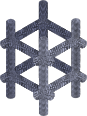
(a)

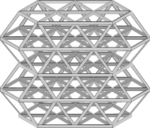
(b)

Figure 1: Typical advanced materials and structures in Engineering Science: (a) carbon nanotube network (Zhang et al., 2018), (b) polymer-metal micro-truss (Juarez et al., 2018).

Small-size structures as carbon nanotube networks (Zhang et al., 2018), 3D-printed polymer-metal micro-trusses (Juarez et al., 2018) and ceramic nanolattices (Meza et al., 2014) are attracting a considerable interest for remarkable features not obtainable by standard materials. Properties as high-thermal conductivity, excellent mechanical strength, electrical conductivity, high-strain sensitivity and large surface area make carbon nanotube networks (Zhang et al., 2018) ideally suitable for the next generation of thermal management (Fasano et al., 2015) and electronic nanodevices (Lee et al., 2016), strain sensors (Chao et al., 2020) and hydrogen storage (Ozturk et al., 2015; Bi et al., 2020). Polymer-metal micro-trusses exhibit enhanced strength, conductivity and electrochemical properties, while ceramic nanolattices feature highest strength- and stiffness-to-weight ratios (Zhang et al., 2020b). In view of promising applications in a large number of fields of Engineering Science, great attention is currently devoted to small-size structures (Ghayesh and Farajpour, 2019); for an insight, typical geometries currently under investigation are shown in Figure 1.

There exist accurate yet computationally very demanding mechanical models of small-size structures, e.g. those involving molecular dynamics simulation for carbon nanotube networks (Barretta et al., 2017; Genoese et al., 2017). On the other hand, several studies have focused on developing analytical or numerical models of small-size continua, which may provide rigorous insight into the essential mechanics of the system and be readily implementable for design and optimization at a relatively-low computational effort. For this purpose, a typical approach is the formulation of continua enriched with nonlocal terms capable of capturing size effects that, instead, cannot be described by the free-scale local continuum approach. Now, nonlocal theories represent a rather established approach to investigate small-size continua. Among others, typical examples are Eringen’s integral theory (Eringen, 1972, 1983), strain-gradient theories (Aifantis, 1999, 2003, 2009, 2011; Askes and Aifantis, 2011; Challamel et al., 2016; Polizzotto, 2014, 2015), micropolar “Cosserat” theory (Lakes, 1991), peridynamic theory (Silling, 2000; Silling et al., 2007) and mechanically-based approaches involving long-range interactions among non-adjacent volumes (Di Paola et al., 2010). Surveys of progress regarding nonlocal elasticity and generalized continua can be found in (Romano and Diaco, 2020) and (Romano et al., 2016), respectively.

Most of the existing nonlocal theories have developed nonlocal models of $1$D and $2$D structures, whose statics and dynamics have been investigated under various boundary conditions in a considerable number of studies, such as: (Akgöz and Civalek, 2013; Attia and Abdel Rahman, 2018; Challamel, 2018; Dastjerdi and Akgöz, 2019; Di Paola et al., 2009, 2013; Farajpour et al., 2018; Fuschi et al., 2019; Ghayesh et al., 2019; Gholipour and Ghayesh, 2020; Karami and Janghorban, 2020; Khaniki, 2019; Li et al., 2018, 2020; Malikan et al., 2020; Numanoğlu et al., 2018; Pinnola et al., 2020a; She et al., 2019; Srividhya et al., 2018; Zhang and Liu, 2020). In this context, an effective approach is the so-called stress-driven nonlocal model, relying on the idea that elastic deformation fields are output of convolution integrals between stress fields and appropriate averaging kernel (Romano and Barretta, 2017a). Nonlocal integral convolution, endowed with the special bi-exponential kernel, can be conveniently replaced with a higher-order differential equation supplemented with non-standard constitutive boundary conditions. The stress-driven theory leads to well-posed structural problems (Romano and Barretta, 2017b), does not exhibit paradoxical results typical of alternative nonlocal beam models (Challamel and Wang, 2008; Demir and Civalek, 2017; Fernández-Sáez et al., 2016) and, in the last few years, has gained increasing popularity for consistency, robustness and ease of implementation. Stress-driven nonlocal theory of elasticity has been applied to several problems of nanomechanics, as witnessed by recent contributions regarding buckling (Oskouie et al., 2018b; Darban et al., 2020), bending (Oskouie et al., 2018a, c; Zhang et al., 2020a; Roghani and Rouhi, ), axial (Barretta et al., 2019a) and torsional responses (Barretta et al., 2018) of nano-beams and elastostatic behaviour of nano-plates (Barretta et al., 2019b; Farajpour et al., 2020).

Nonlocal finite-element formulations have been proposed, in general to discretize single beams or rods (Marotti de Sciarra, 2014; Aria and Friswell, 2019; Alotta et al., 2014, 2017a, 2017b). A very recent study, however, has posed the issue of addressing the dynamics of small-size 2D frames/trusses (Numanoğlu and Civalek, 2019), made by assembling nonlocal beams/rods. Eringen’s differential law has been adopted and the principle of virtual work has been used to derive separate stiffness and mass matrices of a two-node nonlocal element. Typical shape functions of a two-node local element have been exploited, with bending modelled by Bernoulli-Euler kinematic theory. A further recent contribution in this field has been given by Hozhabrossadati et al. (2020), who developed a two-node six-degree-of-freedom beam element for free-vibrations of 3D nano-grids. Separate stiffness and mass matrices have been derived treating axial, bending and torsional responses by Eringen’s differential law and weighted residual method.

However, the studies by Numanoğlu and Civalek (2019) and Hozhabrossadati et al. (2020), dealing with dynamics of nanostructural systems via nonlocal finite elements, are based on Eringen’s differential formulation which leads to mechanical paradoxes and unviable elastic responses (Peddieson et al., 2003), a conclusion acknowledged by the community of Engineering Science (Fernández-Sáez et al., 2016). Lack of alternative technically significant contributions on the matter may also be attributed to the fact that not all size-dependent theories allow for formulating stiffness, mass matrices and nodal forces to be assembled in $2$D and $3$D frames/trusses. As a matter of fact, there is a great interest in developing accurate and computationally-effective nonlocal models of complex nanostructures in view of their increasing relevance in several engineering fields: carbon nanotube networks (Zhang et al., 2018), polymer-metal micro-trusses (Juarez et al., 2018), ceramic nanolattices (Meza et al., 2014). Various examples of nano/micro-scale hierarchical lattice structures and cellular nanostructures have been pointed out by Numanoğlu and Civalek (2019) along with several related applications.

This paper proposes an effective approach to model and assess the dynamic behaviour of complex small-size frames, exploiting the treatment by Romano and Barretta (2017a) confined to straight nano-beams. Key novelties are as follows.

1. Adoption of a well-posed and experimentally consistent stress-driven nonlocal formulation to capture size effects within the members of the structure, assuming uncoupled axial and bending motions (small displacements).

2. Derivation of the exact dynamic stiffness matrix of a two-node stress-driven nonlocal element, from which the global dynamic stiffness matrix of the structure can be readily built by a standard finite-element assembly procedure.

Upon constructing the global dynamic stiffness matrix, all natural frequencies and related modes of the structure are calculated using the Wittrick-Williams (WW) algorithm. The formulation applies not only to frames, but also to trusses. It is presented for 2D frames and is readily extendable to 3D networks of nanotechnological interest.

The main advantages of the proposed approach are summarized as follows. The stress-driven methodology is not affected by inconsistencies and paradoxes corresponding to alternative nonlocal models (Romano et al., 2017). The dynamic-stiffness approach captures the exact dynamic response, using a single two-node beam element for every frame member without any internal mesh. Further, the WW algorithm provides all natural frequencies exactly, without missing anyone and including multiple ones.

The paper is organized as follows. The stress-driven nonlocal formulation for axial and bending motions is described in Section 2. The exact dynamic stiffness matrix of two-node stress-driven nonlocal truss and beam elements is established in Section 3. In addition, the assembly procedure to build the global dynamic stiffness matrix of arbitrarily-shaped small-size frames is illustrated therein. The implementation of the WW algorithm is discussed in Section 4. Numerical applications are presented in Section 5, investigating the role of size effects on the free-vibration responses of small-size 2D structures of current technical interest.

2 Stress-driven nonlocal integral elasticity

This Section introduces fundamental equations governing axial and bending vibrations of a nonlocal beam, according to the stress-driven model recently introduced by Romano and Barretta (2017a, b). Specifically, axial and bending responses are uncoupled on the assumption of small displacements.

Consider a plane beam of length $L$, uniform cross section of area $A$ and moment of inertia $I$, as shown in Fig. 2. Let $E$ be the local elastic stiffness at the macroscopic scale.

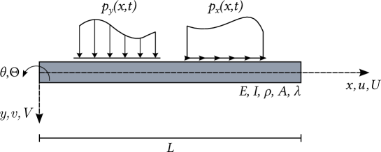
Figure 2: Stress-driven nonlocal beam in axial and bending vibrations.

According to the stress-driven model, the uniaxial strain-stress relationship reads:

$$\varepsilon(x,t)=\frac{1}{E}\int_{0}^{L}\Phi(|x-\zeta|)\sigma(\zeta,t)d\zeta$$ (1)

where $\varepsilon$ is the elastic longitudinal strain, $\sigma$ is the normal stress, $\Phi(|x-\zeta|)$ is a scalar function known as attenuation function assumed to fullfil positivity, symmetric and limit impulsivity.

First, let us focus on the axial response of the beam in Fig. (2). On the assumption that cross sections remain plane and normal to the longitudinal axis, from Eq. (1) the following equation can be derived between longitudinal generalized strain $\gamma$ and axial force $N$ (Barretta et al., 2019a):

$$\gamma(x,t)=\frac{1}{EA}\int_{0}^{L}\Phi(|x-\zeta|)N(\zeta,t)d\zeta$$ (2)

being

$$\gamma(x,t)=u^{(1)}(x,t)$$ (3)

where $u$ is the axial displacement and superscript $(k)$ means $k^{\mathrm{th}}$ derivative w.r.t. the spatial coordinate $x$. As in recent works (Romano and Barretta, 2017a, b; Barretta et al., 2019a), $\Phi$ is taken as the following bi-exponential function:

$$\Phi(x,\zeta)=\frac{1}{2L_{c}}\exp\left(-\frac{|x-\zeta|}{L_{c}}\right)$$ (4)

where $L_{c}=\lambda\cdot L$ is the characteristic length, being $\lambda$ a material-dependent parameter. Eq. (4) fulfils the requirements of symmetry and positivity. Moreover, Eq. (4) satisfies the property of limit impulsivity, i.e. reverts to the Dirac’s delta function for $\lambda\rightarrow 0$, so that Eq. (2) reduces to the standard local constitutive law of linear elasticity at internal points of the structural domain. The choice of Eq. (4) for $\Phi$ is motivated by the fact that, using integration by parts, the integral constitutive law (2) can be now reverted to the following equivalent differential equation:

$$N(x,t)=-EA\cdot L_{c}^{2}\left(\gamma^{(2)}(x,t)-\frac{1}{L_{c}^{2}}\gamma(x,t)\right)$$ (5)

with the additional constitutive BCs

$$\gamma^{(1)}(0,t)=\frac{1}{L_{c}}\gamma(0,t)$$ (6a,b)

$$\gamma^{(1)}(L,t)=-\frac{1}{L_{c}}\gamma(L,t)$$

Next, consider the equilibrium equation governing the axial vibration response (see Fig. 3a)

$$N^{(1)}(x,t)+p_{x}(x,t)-\rho A\ddot{u}(x,t)=0$$ (7)

where $\rho$ is the volume mass density of the material, $p_{x}(x,t)$ is the external transversal force per unit length. Combining Eq. (7) with Eq. (5) leads to the following partial differential equation governing axial vibrations of a stress-driven nonlocal beam:

$$-EA\cdot L_{c}^{2}\left(u^{(4)}(x,t)-\frac{1}{L_{c}^{2}}u^{(2)}(x,t)\right)+p_{x}(x,t)-\rho A\ddot{u}(x,t)=0$$ (8)

Eq. (8) is a partial differential equation in the unknown time-dependent axial displacement $u$, to be solved enforcing the two classical static/kinematic BCs and the additional constitutive BCs (6a,b) together with the initial conditions. As $\lambda\rightarrow 0$, Eq. (8) reverts to the classical partial differential equation governing axial vibrations of the local beam.

Further, for the purposes of this study, it is of interest to formulate the equations governing bending vibrations of the stress-driven nonlocal beam. Assuming the Bernoulli-Euler beam model, Eq. (1) leads to the following nonlocal relation between elastic curvature $\chi$ and bending moment interaction $M$ (Romano and Barretta, 2017a, b)

$$\chi(x,t)=\frac{1}{EI}\int_{0}^{L}\Phi(|x-\zeta|)M(\zeta,t)d\zeta$$ (9)

In Eq. (9)

$$\chi(x,t)=-v^{(2)}(x,t),\qquad\theta(x,t)=-v^{(1)}(x,t)$$ (10a,b)

where $v$ is the deflection in the $y$ direction, $\theta$ is the rotation (positive counterclockwise). Again, using the bi-exponential function (4) in Eq. (9) and integrating by parts leads to the equivalent differential problem of Eq. (9):

$$M(x)=-EI\cdot L_{c}^{2}\left(\chi^{(2)}(x)-\frac{1}{L_{c}^{2}}\chi(x)\right)$$ (11)

with the additional constitutive BCs

$$\chi^{(1)}(0,t)=\frac{1}{L_{c}}\chi(0,t)$$ (12a,b)

$$\chi^{(1)}(L,t)=-\frac{1}{L_{c}}\chi(L,t)$$

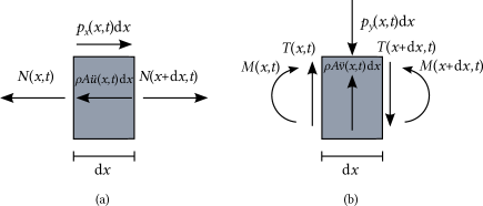
Figure 3: Equilibrium of a beam segment: axial problem (a), bending problem (b).

Next, consider that the bending vibration response of a Bernoulli-Euler beam is governed by the differential condition of equilibrium

$$M^{(2)}(x,t)+p_{y}(x,t)-\rho A\ddot{v}(x,t)=0$$ (13)

where $p_{y}(x,t)$ is the external transverse force per unit length; further,

$$M^{(1)}(x,t)=T(x,t)$$ (14)

as shown in Fig. 3b. Combining Eq. (11) and Eq. (13) leads to the following equation governing bending vibrations of a stress-driven nonlocal beam:

$$EI\cdot L_{c}^{2}\left(v^{(6)}(x,t)-\frac{1}{L_{c}^{2}}v^{(4)}(x,t)\right)+p_{y}(x,t)-\rho A\ddot{v}(x,t)=0$$ (15)

Eq. (15) is a partial differential equation in the unknown time-dependent deflection $v$, to be solved enforcing the classical four static/kinematic BCs and the two constitutive BCs (12a,b) (Romano and Barretta, 2017a, b), together with the initial conditions. Note that, as $\lambda\rightarrow 0$, Eq. (15) reverts to the classical partial differential equation governing the local Bernoulli-Euler beam.

Eq. (8) and Eq. (15) are the basis to derive the exact dynamic stiffness of a two-node stress-driven nonlocal beam element, as explained in the next Section.

3 Exact dynamic stiffness matrix of stress-driven nonlocal beam elements

Let us consider the stress-driven nonlocal beam in Fig. 4, acted upon by harmonic forces/moments at the ends.

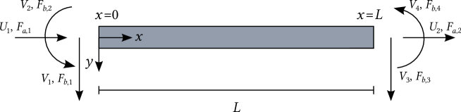
Figure 4: Nodal forces and displacements of a two-node stress-driven nonlocal beam element.

Beam ends are referred to as “nodes” with three degrees of freedom each and the beam as a two-node stress-driven nonlocal beam element. Denoting by $u(x,t)=U(x)\mathrm{e}^{\mathrm{i}\omega t}$, $v(x,t)=V(x)\mathrm{e}^{\mathrm{i}\omega t}$, $\theta(x,t)=\Theta(x)\mathrm{e}^{\mathrm{i}\omega t}$, …, axial and bending response variables, be $\mathbf{F}\mathrm{e}^{\mathrm{i}\omega t}=[-N(0)\;N(L)\;-T(0)\;-M(0)\;T(L)\;M(L)]^{\mathrm{T}}\mathrm{e}^{\mathrm{i}\omega t}$ the vector of nodal forces and $\mathbf{U}\mathrm{e}^{\mathrm{i}\omega t}=[U(0)\;U(L)\;V(0)\;\Theta(0)\;V(L)\;\Theta(L)]^{\mathrm{T}}\mathrm{e}^{\mathrm{i}\omega t}$ the corresponding vector of nodal displacements.

For generality, the dynamic stiffness matrix of the two-node stress-driven nonlocal beam element is sought in terms of dimensionless frequencies (Banerjee and Williams, 1996; Banerjee, 1998, 2001, 2003). Thus, the equations of motion (8) and (15) governing steady-state responses under harmonic forces/moments at beam ends and the associated constitutive BCs (6a,b) and (12a,b) are rewritten as ($\omega$ – dependence of the response variables is omitted for brevity):

$$(\mathcal{L}_{a}+\overline{\omega}_{a}^{2}\mathcal{I})[U]=0\,,\qquad\textrm{with}\qquad\mathcal{L}_{a}:=-\lambda^{2}\frac{{\mathrm{d}^{4}}}{\mathrm{d}\xi^{4}}+\frac{{\mathrm{d}^{2}}}{\mathrm{d}\xi^{2}}\,,\quad\xi\in[0,1]$$ (16)

$$\left.\frac{\mathrm{d}\Gamma}{\mathrm{d}\xi}\right\rvert_{\xi=0}=\frac{1}{\lambda}\Gamma(0)$$ (17a,b)

$$\left.\frac{\mathrm{d}\Gamma}{\mathrm{d}\xi}\right\rvert_{\xi=1}=-\frac{1}{\lambda}\Gamma(1)$$

$$(\mathcal{L}_{b}+\overline{\omega}_{b}^{4}\mathcal{I})[V]=0\,,\qquad\textrm{with}\qquad\mathcal{L}_{b}:=\lambda^{2}\frac{{\mathrm{d}^{6}}}{\mathrm{d}\xi^{6}}-\frac{{\mathrm{d}^{4}}}{\mathrm{d}\xi^{4}}\,,\quad\xi\in[0,1]$$ (18)

$$\left.\frac{\mathrm{d}X}{\mathrm{d}\xi}\right\rvert_{\xi=0}=\frac{1}{\lambda}X(0)$$ (19a,b)

$$\left.\frac{\mathrm{d}X}{\mathrm{d}\xi}\right\rvert_{\xi=1}=-\frac{1}{\lambda}X(1)$$

where $\,\xi=x/L\,$, $\,\lambda=L_{c}/L\,$, $\,\overline{\omega}_{a}=[\rho A(\omega L)^{2}/EA]^{1/2}\,$, $\,\overline{\omega}_{b}=[\rho A(\omega L^{2})^{2}/EI]^{1/4}\,$ and $\,\mathcal{I}\,$ is the identity map. Further, in Eq. (16) through Eqs. (19a,b), the notation $\mathrm{d}^{k}/\mathrm{d}\xi^{k}$ distinguishes the derivative w.r.t. to the dimensionless spatial coordinate $\xi$ from the derivative w.r.t. to $x$, indicated by the superscript $(k)$. Upon enforcing the constitutive BCs (17a,b) and (19a,b), the exact solutions of Eq. (16) and Eq. (18) can be obtained in the following analytical forms:

$$U(\xi)=\sum_{k=1}^{2}c_{a,k}f_{k}(\xi)$$ (20)

$$V(\xi)=\sum_{k=1}^{4}c_{b,k}g_{k}(\xi)$$ (21)

where $c_{a,k}$ for $k=1,2$ and $c_{b,k}$ for $k=1,...,4$ are integration constants depending on the classical static/kinematic BCs. Further, $f_{k}(\xi)=f_{k}(\xi,\overline{\omega}_{a})$ and $g_{k}(\xi)=g_{k}(\xi,\overline{\omega}_{b})$ are closed analytical functions depending on frequency and parameters of the stress-driven nonlocal beam, reported in Appendix A for brevity.

Now, from Eq. (20) and Eq. (21) and taking into account Eqs. (10a,b), Eq. (11) and Eq. (14) for the bending response, as well as Eq. (3) and Eq. (5) for the axial response, the whole set of response variables can be cast as functions of the integration constants $\mathbf{c}_{a}=[c_{a,1}\;c_{a,2}]^{T}$ and $\mathbf{c}_{b}=[c_{b,1}\;c_{b,2}\;c_{b,3}\;c_{b,4}]^{T}$, i.e.

$$U=U(\xi,\mathbf{c}_{a})$$ (22a-f)

$$N=-\frac{EA\cdot\lambda^{2}}{L}\left(\frac{{\mathrm{d}^{3}U}}{\mathrm{d}\xi^{3}}-\frac{1}{\lambda^{2}}\frac{\mathrm{d}U}{\mathrm{d}\xi}\right)=N(\xi,\mathbf{c}_{a})$$

$$V=V(\xi,\mathbf{c}_{b})$$

$$\Theta=-\frac{\mathrm{d}V}{\mathrm{d}\xi}=\Theta(\xi,\mathbf{c}_{b})$$

$$M=\frac{EI\cdot\lambda^{2}}{L^{2}}\left(\frac{{\mathrm{d}^{4}V}}{\mathrm{d}\xi^{4}}-\frac{1}{\lambda^{2}}\frac{{\mathrm{d}^{2}V}}{\mathrm{d}\xi^{2}}\right)=M(\xi,\mathbf{c}_{b})$$

$$T=\frac{EI\cdot\lambda^{2}}{L^{3}}\left(\frac{{\mathrm{d}^{5}V}}{\mathrm{d}\xi^{5}}-\frac{1}{\lambda^{2}}\frac{{\mathrm{d}^{3}V}}{\mathrm{d}\xi^{3}}\right)=T(\xi,\mathbf{c}_{b})$$

Computing Eqs. (22a-f) at $\xi=0$ and $\xi=1$, the following expressions are obtained for the vectors of nodal displacements and forces:

$$\mathbf{U}=\mathbf{A}\mathbf{c}$$ (23)

$$\mathbf{F}=\mathbf{B}\mathbf{c}$$ (24)

where $\mathbf{c}=[\mathbf{c}_{a}\;\mathbf{c}_{b}]^{\mathrm{T}}$. Next, using Eq. (23) to calculate $\mathbf{c}=\mathbf{A}^{-1}\mathbf{U}$ and replacing for $\mathbf{c}$ in Eq. (24) lead to (Banerjee, 1997)

$$\mathbf{B}\mathbf{A}^{-1}\mathbf{U}=\mathbf{D}\mathbf{U}=\mathbf{F}$$ (25)

where

$$\mathbf{D}(\omega)=\begin{bmatrix}\mathbf{D}_{a}(\overline{\omega}_{a}(\omega))&\mathbf{0}\\ \mathbf{0}&\mathbf{D}_{b}(\overline{\omega}_{b}(\omega))\\ \end{bmatrix}$$ (26)

being $\mathbf{D}_{a}$ and $\mathbf{D}_{b}$ the block matrices associated with axial and bending responses, respectively. The matrix $\mathbf{D}$ in Eq. (26) is the dynamic stiffness matrix of the two-node stress-driven nonlocal beam element in Fig. 3. Remarkably, it is available in a closed analytical form, as the inverse matrix $\mathbf{A}^{-1}$ in Eq. (25) can be obtained symbolically from the inverses of the two separate block matrices associated with axial and bending responses (Failla, 2016). The matrix $\mathbf{D}$ is exact, because is based on the exact solutions of the equations of motion (16) and (18) along with the related constitutive BCs (17a,b) and (19a,b). Indeed, no approximations have been made in building the solutions (20) and (21).

An alternative approach to derive the exact dynamic stiffness matrix of the two-node stress-driven nonlocal beam element in Fig. 4 relies on the principle of virtual work. Consider Eq. (16) governing the steady-state axial vibrations under harmonic axial forces at the beam ends (see Fig. 4). The identity of internal and external works reads ($\overline{\omega}_{a}$ – dependence of response variables and virtual axial displacement/longitudinal generalized strain is omitted for brevity)

$$L\int_{0}^{1}\left(-\lambda^{2}\frac{{\mathrm{d}^{3}U}}{\mathrm{d}\xi^{3}}+\frac{\mathrm{d}U}{\mathrm{d}\xi}\right)\delta\Gamma~{}~{}\mathrm{d}\xi-\overline{\omega}_{a}^{2}L\int_{0}^{1}U\delta U~{}~{}\mathrm{d}\xi=\widetilde{F}_{a,1}\delta U_{1}+\widetilde{F}_{a,2}\delta U_{2}$$ (27)

where $\delta U_{k}$ for $k=1,2$ are virtual nodal displacements, $\delta U$ and $\delta\Gamma=\mathrm{d}\delta U/\mathrm{d}\xi$ the corresponding virtual axial displacement and longitudinal generalized strain along the beam; further, $\widetilde{F}_{a,k}=(L^{2}/EA)F_{a,k}$ for $k=1,2$. Now, exact expression of the axial displacement $U$ is

$$U(\xi)=\sum_{j=1}^{2}U_{j}\psi_{j}(\xi)$$ (28)

where $U_{j}$ are the nodal displacements associated with the applied nodal forces $\widetilde{F}_{a,k}$ and $\psi_{j}$ are frequency-dependent, exact shape functions obtained from Eq. (20) enforcing the following BCs (omitting $\overline{\omega}_{a}$ – dependence for brevity)

$$U(0)=1\qquad U(1)=0 \rightarrow \psi_{1}(\xi)$$ (29)

$$U(0)=0\qquad U(1)=1 \rightarrow \psi_{2}(\xi)$$

The boundary value problem (29) requires inverting a $2\times 2$ matrix to calculate the integration constants $c_{a,k}$ in Eq. (20) and the matrix inversion can be readily implemented in a closed form. Replacing Eq. (28) in Eq. (27) and enforcing the identity of internal and external works for any virtual nodal displacements leads to

$$\sum_{j=1}^{2}\left(L\int_{0}^{1}\left(-\lambda^{2}\frac{\mathrm{d}\psi_{i}}{\mathrm{d}\xi}\frac{{\mathrm{d}^{3}\psi_{j}}}{\mathrm{d}\xi^{3}}+\frac{\mathrm{d}\psi_{i}}{\mathrm{d}\xi}\frac{\mathrm{d}\psi_{j}}{\mathrm{d}\xi}\right)~{}~{}\mathrm{d}\xi\right)U_{j}-\sum_{j=1}^{2}\left(\overline{\omega}_{a}^{2}L\int_{0}^{1}\psi_{i}\psi_{j}~{}~{}\mathrm{d}\xi\right)U_{j}=\widetilde{F}_{a,1}\psi_{i}(0)$$ (30)

$$+\widetilde{F}_{a,2}\psi_{i}(1)$$

where $\psi_{1}(1)=\psi_{2}(0)=0$ on the r.h.s. Eq. (30) can be written in matrix form as

$$\widetilde{\mathbf{D}}_{a}(\overline{\omega}_{a})\mathbf{U}_{a}=\widetilde{\mathbf{F}}_{a}$$ (31)

where $\mathbf{U}_{a}=\begin{bmatrix}U_{1}&U_{2}\end{bmatrix}^{\mathrm{T}}$, $\widetilde{\mathbf{F}}_{a}=\begin{bmatrix}\widetilde{F}_{a,1}&\widetilde{F}_{a,2}\end{bmatrix}^{\mathrm{T}}$ and $\widetilde{\mathbf{D}}_{a}$ is a $2\times 2$ matrix with elements

$$(\widetilde{\mathbf{D}}_{a})_{ij}=L\int_{0}^{1}\left(-\lambda^{2}\frac{\mathrm{d}\psi_{i}}{\mathrm{d}\xi}\frac{{\mathrm{d}^{3}\psi_{j}}}{\mathrm{d}\xi^{3}}+\frac{\mathrm{d}\psi_{i}}{\mathrm{d}\xi}\frac{\mathrm{d}\psi_{j}}{\mathrm{d}\xi}\right)~{}\mathrm{d}\xi-\overline{\omega}_{a}^{2}L\int_{0}^{1}\psi_{i}\psi_{j}~{}~{}\mathrm{d}\xi$$ (32)

Being $\widetilde{\mathbf{F}}_{a}=(L^{2}/EA)\mathbf{F}_{a}$ for $\mathbf{F}_{a}=\begin{bmatrix}F_{a,1}&F_{a,2}\end{bmatrix}^{\mathrm{T}}$, we finally obtain

$$\mathbf{D}_{a}(\overline{\omega}_{a})\mathbf{U}_{a}=\mathbf{F}_{a}$$ (33)

where $\mathbf{D}_{a}$ is the dynamic stiffness matrix of the rod. Next, consider Eq. (18) governing the steady-state bending vibrations under transverse forces/moments applied at the beam ends (Fig. 4). The identity of internal and external works reads ($\overline{\omega}_{b}$ – dependence of response variables and virtual deflection/curvature is omitted for conciseness)

$$L\int_{0}^{1}\left(\lambda^{2}\frac{{\mathrm{d}^{4}V}}{\mathrm{d}\xi^{4}}-\frac{{\mathrm{d}^{2}V}}{\mathrm{d}\xi^{2}}\right)\delta X~{}\mathrm{d}\xi-\overline{\omega}_{b}^{4}L\int_{0}^{1}V\delta V~{}~{}\mathrm{d}\xi=\widetilde{F}_{b,1}\delta V_{1}+\widetilde{F}_{b,2}\delta V_{2}+\widetilde{F}_{b,3}\delta V_{3}+\widetilde{F}_{b,4}\delta V_{4}$$ (34)

where $\delta V_{k}$ for $k=1,...,4$ are virtual nodal displacements, $\delta V$ and $\delta X=-\mathrm{d}^{2}\delta V/\mathrm{d}\xi^{2}$ the corresponding virtual deflection and curvature along the beam; further, $\widetilde{F}_{b,k}=(L^{4}/EI)F_{b,k}$ for $k=1,3$ and $\widetilde{F}_{b,k}=(L^{3}/EI)F_{b,k}$ for $k=2,4$, hence:

$$\underbrace{\begin{bmatrix}\widetilde{F}_{b,1}\\ \widetilde{F}_{b,2}\\ \widetilde{F}_{b,3}\\ \widetilde{F}_{b,4}\end{bmatrix}}_{\widetilde{\mathbf{F}}_{b}}=\underbrace{\begin{bmatrix}\frac{L^{4}}{EI}&0&0&0\\ 0&\frac{L^{3}}{EI}&0&0\\ 0&0&\frac{L^{4}}{EI}&0\\ 0&0&0&\frac{L^{3}}{EI}\end{bmatrix}}_{\mathbf{T}}\underbrace{\begin{bmatrix}F_{b,1}\\ F_{b,2}\\ F_{b,3}\\ F_{b,4}\\ \end{bmatrix}}_{\mathbf{F}_{b}}$$ (35)

The exact expression of the deflection $V$ is

$$V(\xi)=\sum_{j=1}^{4}V_{j}\beta_{j}(\xi)$$ (36)

$V_{j}$ are the nodal displacements associated with the applied nodal forces/moments $F_{b,k}$ and $\beta_{j}$ are frequency-dependent, exact shape functions obtained from Eq. (21) by enforcing the following BCs (again, omitting $\overline{\omega}_{b}$ – dependence for brevity)

$$U(0)=1\qquad\Theta(0)=0\qquad U(1)=0\qquad\Theta(1)=0 \rightarrow \beta_{1}(\xi)$$ (37)

$$U(0)=0\qquad\Theta(0)=1\qquad U(1)=0\qquad\Theta(1)=0 \rightarrow \beta_{2}(\xi)$$

$$U(0)=0\qquad\Theta(0)=0\qquad U(1)=1\qquad\Theta(1)=0 \rightarrow \beta_{3}(\xi)$$

$$U(0)=0\qquad\Theta(0)=0\qquad U(1)=0\qquad\Theta(1)=1 \rightarrow \beta_{4}(\xi)$$

The boundary value problem (37) requires inverting a $4\times 4$ matrix to calculate the integration constants $c_{b,k}$ in Eq. (21), and the matrix inversion can be readily implemented in closed form (Failla, 2016). Replacing Eq. (36) in Eq. (34) and enforcing the identity of internal and external works for any virtual nodal displacements yields

$$\sum_{j=1}^{4}\left(L\int_{0}^{1}-\lambda^{2}\frac{{\mathrm{d}^{2}\beta_{i}}}{\mathrm{d}\xi^{2}}\frac{{\mathrm{d}^{4}\beta_{j}}}{\mathrm{d}\xi^{4}}+\frac{{\mathrm{d}^{2}\beta_{i}}}{\mathrm{d}\xi^{2}}\frac{{\mathrm{d}^{2}\beta_{j}}}{\mathrm{d}\xi^{2}}~{}\mathrm{d}\xi\right)V_{j}-\sum_{j=1}^{4}\left(\overline{\omega}_{b}^{4}L\int_{0}^{1}\beta_{i}\beta_{j}~{}~{}\mathrm{d}\xi\right)V_{j}=\widetilde{F}_{b,1}\beta_{i}(0)$$ (38)

$$-\widetilde{F}_{b,2}\left.\frac{\mathrm{d}\beta_{i}}{\mathrm{d}\xi}\right\rvert_{\xi=0}+\widetilde{F}_{b,3}\beta_{i}(1)-\widetilde{F}_{b,4}\left.\frac{\mathrm{d}\beta_{i}}{\mathrm{d}\xi}\right\rvert_{\xi=1}$$

being $\beta_{i}(0)=\left.\frac{\mathrm{d}\beta_{i}}{\mathrm{d}\xi}\right\rvert_{\xi=0}=0$ and $\beta_{i}(1)=\left.\frac{\mathrm{d}\beta_{i}}{\mathrm{d}\xi}\right\rvert_{\xi=1}=0$ except for $\beta_{1}(0)=1$, $\left.\frac{\mathrm{d}\beta_{2}}{\mathrm{d}\xi}\right\rvert_{\xi=0}=-1$, $\beta_{3}(1)=1$, $\left.\frac{\mathrm{d}\beta_{4}}{\mathrm{d}\xi}\right\rvert_{\xi=1}=-1$. Eq. (38) can be written in matrix form as

$$\widetilde{\mathbf{D}}_{b}(\overline{\omega}_{b})\mathbf{U}_{b}=\widetilde{\mathbf{F}}_{b}$$ (39)

where $\mathbf{U}_{b}=\begin{bmatrix}V_{1}&V_{2}&V_{3}&V_{4}\end{bmatrix}^{\mathrm{T}}$, $\widetilde{\mathbf{F}}_{b}=\begin{bmatrix}\widetilde{F}_{b,1}&\widetilde{F}_{b,2}&\widetilde{F}_{b,3}&\widetilde{F}_{b,4}\end{bmatrix}^{\mathrm{T}}$ and $\widetilde{\mathbf{D}}_{b}$ is a $4\times 4$ matrix whose elements are

$$(\widetilde{\mathbf{D}}_{b})_{ij}=L\int_{0}^{1}-\lambda^{2}\frac{{\mathrm{d}^{2}\beta_{i}}}{\mathrm{d}\xi^{2}}\frac{{\mathrm{d}^{4}\beta_{j}}}{\mathrm{d}\xi^{4}}+\frac{{\mathrm{d}^{2}\beta_{i}}}{\mathrm{d}\xi^{2}}\frac{{\mathrm{d}^{2}\beta_{j}}}{\mathrm{d}\xi^{2}}~{}\mathrm{d}\xi-\overline{\omega}_{b}^{4}L\int_{0}^{1}\beta_{i}\beta_{j}~{}~{}\mathrm{d}\xi$$ (40)

From Eq. (40) and taking into account Eq. (35), we finally obtain

$$\mathbf{D}_{b}(\overline{\omega}_{b})\mathbf{U}_{b}=\mathbf{F}_{b}$$ (41)

being

$$\mathbf{D}_{b}(\overline{\omega}_{b})=\mathbf{T}^{-1}\widetilde{\mathbf{D}}_{b}$$ (42)

where $\mathbf{T}^{-1}$ is trivially computable. Now, assembling Eq. (32) and Eq. (40) for axial and bending vibrations yields

$$\mathbf{D}\mathbf{U}=\mathbf{F}\qquad\mathbf{D}(\omega)=\begin{bmatrix}\mathbf{D}_{a}(\overline{\omega}_{a})&\mathbf{0}\\ \mathbf{0}&\mathbf{D}_{b}(\overline{\omega}_{b})\end{bmatrix}$$ (43)

where

$$\mathbf{U}=\begin{bmatrix}U_{1}&U_{2}&V_{1}&V_{2}&V_{3}&V_{4}\end{bmatrix}^{\mathrm{T}}\qquad\mathbf{F}=\begin{bmatrix}F_{a,1}&F_{a,2}&F_{b,1}&F_{b,2}&F_{b,3}&F_{b,4}\end{bmatrix}^{\mathrm{T}}$$ (44a,b)

Remarkably, upon calculating the integrals (32) and (40) by standard numerical methods, the matrix $\mathbf{D}$ in Eq. (43) is found to coincide with the dynamic stiffness matrix $\mathbf{D}$ in Eq. (26).

It is noteworthy that all elements of the dynamic stiffness matrix $\mathbf{D}$ are real. Further, $\mathbf{D}$ is symmetric. Indeed, performing integration by parts of Eq. (32) yields

$$(\widetilde{\mathbf{D}}_{a})_{ij}=L\int_{0}^{1}\left(\lambda^{2}\frac{{\mathrm{d}^{2}\psi_{i}}}{\mathrm{d}\xi^{2}}\frac{{\mathrm{d}^{2}\psi_{j}}}{\mathrm{d}\xi^{2}}+\frac{\mathrm{d}\psi_{i}}{\mathrm{d}\xi}\frac{\mathrm{d}\psi_{j}}{\mathrm{d}\xi}\right)~{}\mathrm{d}\xi-\overline{\omega}_{a}^{2}L\int_{0}^{1}\psi_{i}\psi_{j}~{}~{}\mathrm{d}\xi-\left.\lambda^{2}L\frac{\mathrm{d}\psi_{i}}{\mathrm{d}\xi}\frac{{\mathrm{d}^{2}\psi_{j}}}{\mathrm{d}\xi^{2}}\right\rvert_{0}^{1}$$ (45)

The shape functions $\psi_{i}$ fulfil Eqs. (17a,b), i.e.

$$\left.\frac{{\mathrm{d}^{2}\psi_{i}}}{\mathrm{d}\xi^{2}}\right\rvert_{\xi=0}=\frac{1}{\lambda}\left.\frac{\mathrm{d}\psi_{i}}{\mathrm{d}\xi}\right\rvert_{\xi=0}\qquad\left.\frac{{\mathrm{d}^{2}\psi_{i}}}{\mathrm{d}\xi^{2}}\right\rvert_{\xi=1}=-\frac{1}{\lambda}\left.\frac{\mathrm{d}\psi_{i}}{\mathrm{d}\xi}\right\rvert_{\xi=1}$$ (46a,b)

Therefore, in view of Eq. (46a,b) in Eq. (45) takes the form

$$(\widetilde{\mathbf{D}}_{a})_{ij} =L\int_{0}^{1}\left(\lambda^{2}\frac{{\mathrm{d}^{2}\psi_{i}}}{\mathrm{d}\xi^{2}}\frac{{\mathrm{d}^{2}\psi_{j}}}{\mathrm{d}\xi^{2}}+\frac{\mathrm{d}\psi_{i}}{\mathrm{d}\xi}\frac{\mathrm{d}\psi_{j}}{\mathrm{d}\xi}\right)~{}\mathrm{d}\xi-\overline{\omega}_{a}^{2}L\int_{0}^{1}\psi_{i}\psi_{j}~{}~{}\mathrm{d}\xi$$ (47)

$$+\lambda L\left(\left.\frac{\mathrm{d}\psi_{i}}{\mathrm{d}\xi}\frac{\mathrm{d}\psi_{j}}{\mathrm{d}\xi}\right\rvert_{\xi=0}\right.\left.+\left.\frac{\mathrm{d}\psi_{i}}{\mathrm{d}\xi}\frac{\mathrm{d}\psi_{j}}{\mathrm{d}\xi}\right\rvert_{\xi=1}\right)$$

Eq. (47) implies that $(\mathbf{D}_{a})_{ij}=(\mathbf{D}_{a})_{ji}$, i.e the symmetry of the dynamic stiffness matrix associated with the axial response.

Likewise, performing integration by parts of Eq. (40) yields

$$(\widetilde{\mathbf{D}}_{b})_{ij}=L\int_{0}^{1}\left(\lambda^{2}\frac{{\mathrm{d}^{3}\beta_{i}}}{\mathrm{d}\xi^{3}}\frac{{\mathrm{d}^{3}\beta_{j}}}{\mathrm{d}\xi^{3}}+\frac{{\mathrm{d}^{2}\beta_{i}}}{\mathrm{d}\xi^{2}}\frac{{\mathrm{d}^{2}\beta_{j}}}{\mathrm{d}\xi^{2}}\right)~{}\mathrm{d}\xi-\overline{\omega}_{b}^{4}L\int_{0}^{1}\beta_{i}\beta_{j}~{}~{}\mathrm{d}\xi-\left.\lambda^{2}L\frac{{\mathrm{d}^{2}\beta_{i}}}{\mathrm{d}\xi^{2}}\frac{{\mathrm{d}^{3}\beta_{i}}}{\mathrm{d}\xi^{3}}\right\rvert_{0}^{1}$$ (48)

Again, since the shape functions $\beta_{i}$ satisfy Eqs. (19a,b), i.e.

$$\left.\frac{{\mathrm{d}^{3}\beta_{i}}}{\mathrm{d}\xi^{3}}\right\rvert_{\xi=0}=\frac{1}{\lambda}\left.\frac{{\mathrm{d}^{2}\beta_{i}}}{\mathrm{d}\xi^{2}}\right\rvert_{\xi=0}\qquad\left.\frac{{\mathrm{d}^{3}\beta_{i}}}{\mathrm{d}\xi^{3}}\right\rvert_{\xi=1}=-\frac{1}{\lambda}\left.\frac{{\mathrm{d}^{2}\beta_{i}}}{\mathrm{d}\xi^{2}}\right\rvert_{\xi=1}$$ (49a,b)

Eq. (48) can be written as

$$(\widetilde{\mathbf{D}}_{b})_{ij} =L\int_{0}^{1}\left(\lambda^{2}\frac{{\mathrm{d}^{3}\beta_{i}}}{\mathrm{d}\xi^{3}}\frac{{\mathrm{d}^{3}\beta_{j}}}{\mathrm{d}\xi^{3}}+\frac{{\mathrm{d}^{2}\beta_{i}}}{\mathrm{d}\xi^{2}}\frac{{\mathrm{d}^{2}\beta_{j}}}{\mathrm{d}\xi^{2}}\right)~{}\mathrm{d}\xi-\overline{\omega}_{b}^{4}L\int_{0}^{1}\beta_{i}\beta_{j}~{}~{}\mathrm{d}\xi$$ (50)

$$+\lambda L\left(\left.\frac{{\mathrm{d}^{2}\beta_{i}}}{\mathrm{d}\xi^{2}}\frac{{\mathrm{d}^{2}\beta_{j}}}{\mathrm{d}\xi^{2}}\right\rvert_{\xi=0}\right.\left.+\left.\frac{{\mathrm{d}^{2}\beta_{i}}}{\mathrm{d}\xi^{2}}\frac{{\mathrm{d}^{2}\beta_{j}}}{\mathrm{d}\xi^{2}}\right\rvert_{\xi=1}\right)$$

Eq. (50) demonstrates that $(\mathbf{D}_{b})_{ij}=(\mathbf{D}_{b})_{ji}$, that is the dynamic stiffness matrix associated with the bending response is symmetric.

At this stage, a few remarks are in order. The dynamic stiffness matrix $\mathbf{D}$ of the two-node stress-driven beam element in Fig. 4 can be used to build the global dynamic stiffness matrix of an arbitrarily-shaped frame. For this, a standard finite-element assembly procedure can be implemented. It is noteworthy that every frame member is modelled exactly by a single element. The size of the global dynamic stiffness matrix depends only on the total number of degrees of freedom of the frame nodes (“beam-to-column” nodes), as no meshing is required within every frame member.

The global dynamic stiffness matrix is exact because is exact the dynamic stiffness matrix of every frame member. The exact natural frequencies and related modes can be calculated by the WW algorithm, using the implementation described in Section 4.

The frequency response of the frame, acted upon by harmonic forces/moments at the nodes (Banerjee, 1997), can be calculated upon inverting the global dynamic stiffness matrix. This can be done numerically, for every frequency of interest.

The proposed framework can be generalized to build the global dynamic stiffness matrix of 3D frames. This requires formulating the exact dynamic stiffness matrix of a two-node stress-driven nonlocal beam element, where each node features six degrees of freedom including torsional rotation. It is noticed that the stress-driven nonlocal constitutive law for torsional behaviour and associated constitutive BCs, formulated by Barretta et al. (2018), lead to a partial differential equation governing torsional vibrations that mirror Eq. (8) for axial vibrations. Therefore, under the assumption of small displacements, the exact dynamic stiffness matrix of the two-node, twelve-degree-of-freedom stress-driven nonlocal beam element will involve separate block matrices pertinent to axial, bending and torsional responses. Again, the global dynamic stiffness matrix will be obtainable by a standard finite-element assembly procedure.

The global dynamic stiffness matrix of an arbitrarily-shaped truss can be built based on the dynamic stiffness matrix of a two-node rod, which can be readily derived from Eq. (25) upon eliminating rows and columns associated with the bending response. For trusses as well, the exact natural frequencies and modes can be computed by the WW algorithm, as described in Section 4. Both 2D and 3D dimensional truss structures can be modelled.

The proposed framework represents an exact approach to the dynamics of small-size frames/trusses, where size effects are modelled by the stress-driven nonlocal model. Here, the assumption is that the nonlocality introduces a coupling between the responses at different points that belong to the same frame/truss member, to an extent depending on the internal length $\lambda$. Recognize that this assumption is made also in the previous works on small-size frames/trusses (Numanoğlu and Civalek, 2019; Hozhabrossadati et al., 2020), where Eringen’s differential model (1983) was used to build stiffness and mass matrices of a two-node nonlocal finite element.

The differential operators $\,\mathcal{L}_{a}\,$ and $\,\mathcal{L}_{b}\,$ in Eq. (16) and Eq. (18), governing axial and bending free vibrations of the two-node stress-driven nonlocal beam element in Fig. 4, are self-adjoint. That is,

$$\int_{0}^{1}\mathcal{L}_{a}[U_{m}]U_{n}~{}~{}\mathrm{d}\xi=\int_{0}^{1}\mathcal{L}_{a}[U_{n}]U_{m}~{}~{}\mathrm{d}\xi$$ (51)

$$\int_{0}^{1}\mathcal{L}_{b}[V_{m}]V_{n}~{}~{}\mathrm{d}\xi=\int_{0}^{1}\mathcal{L}_{b}[V_{n}]V_{m}~{}~{}\mathrm{d}\xi$$ (52)

with $U_{m}$, $U_{n}$, $V_{m}$, $V_{n}$ eigenfunctions fulfilling the constitutive BCs (17a,b)-(19a,b) and the static/kinematic BCs. Eq. (51) can be demonstrated writing Eq. (16) for the $m^{\mathrm{th}}$ eigenfunction $U_{m}(\xi)$, multiplying by the $n^{\mathrm{th}}$ eigenfunction $U_{n}(\xi)$ and integrating Eq. (16) over $[0,1]$, performing integration by parts (as to derive Eq. (45)) and enforcing the constitutive BCs (17a,b) along with the static/kinematic BCs. Eq. (52) can be proven likewise, starting from Eq. (18). Furthermore, the self-adjoint differential operators $\mathcal{L}_{a}$ and $\mathcal{L}_{b}$ feature properly-defined Green’s functions, given by:

$$G_{a}(\xi,\xi_{0})=g_{a,1}+g_{a,2}\xi+g_{a,3}\lambda^{2}\mathrm{e}^{-\frac{\xi}{\lambda}}+g_{a,4}\lambda^{2}\mathrm{e}^{\frac{\xi}{\lambda}}+\left[\xi_{0}-\xi+\frac{\lambda}{2}\left(\mathrm{e}^{\frac{\xi-\xi_{0}}{\lambda}}-\mathrm{e}^{-\frac{\xi-\xi_{0}}{\lambda}}\right)\right]\mathcal{H}(\xi-\xi_{0})$$ (53)

$$G_{b}(\xi,\xi_{0})= ~{}~{}g_{b,1}+g_{b,2}\xi+g_{b,3}\xi^{2}+g_{b,4}\xi^{3}+g_{b,5}\lambda^{4}\mathrm{e}^{-\frac{\xi}{\lambda}}+g_{b,6}\lambda^{4}\mathrm{e}^{\frac{\xi}{\lambda}}+\frac{1}{6}\left[\vphantom{\frac{\xi-\xi_{0}}{\lambda}}-(\xi-\xi_{0})^{3}+6\lambda^{2}(\xi-\xi_{0})\right.$$ (54)

$$\left.+6\lambda^{3}\sinh\left(\frac{\xi-\xi_{0}}{\lambda}\right)\right]\mathcal{H}(\xi-\xi_{0})$$

where $g_{a,i}$ (for $i=1,...,4$) and $g_{b,i}$ (for $i=1,...,6$) are integration constants to be evaluated depending on static/kinematic BCs and $\mathcal{H}$ is the unit-step function defined by

$$\mathcal{H}(\xi-\xi_{0})=\left\{\begin{aligned} &1&&\text{if}~{}\xi>\xi_{0}\\ &0&&\text{if}~{}\xi<\xi_{0}\end{aligned}\right.$$ (55)

The Green’s functions (53) and (54) are real functions, obtained as solutions of the equations:

$$\mathcal{L}_{a}[U]+\delta(\xi-\xi_{0})=0$$ (56)

$$\mathcal{L}_{b}[V]+\delta(\xi-\xi_{0})=0$$ (57)

Specifically, Eq.(53) and Eq.(54) are built applying direct and inverse Laplace transform to Eq.(55) and Eq.(56) respectively (for a similar approach, see (Wang and Qiao, 2007)).

Since $\mathcal{L}_{a}$ and $\mathcal{L}_{b}$ are self-adjoint, the (real) Green’s functions are symmetric. Accordingly, the free-vibration problem of the two-node stress-driven nonlocal beam element features an infinite sequence of real eigenvalues (natural frequencies) with associated eigenfunctions, which form an infinite system of functions satisfying the orthogonality conditions (Courant and Hilbert, 1953):

$$L\int_{0}^{1}\rho AU_{m}U_{n}~{}\mathrm{d}\xi=\delta_{mn}$$ (58)

$$L\int_{0}^{1}\rho AV_{m}V_{n}~{}\mathrm{d}\xi=\delta_{mn}$$ (59)

with $\delta_{mn}$ Kronecker delta.

Existence of an infinite sequence of real natural frequencies and associated eigenfunctions follows also for the free-vibration problem of an arbitrarily-shaped frame whose members are two-node stress-driven nonlocal beam elements. Indeed, as motivated below, the free-vibration problem of such a frame is still governed by self-adjoint differential operators with associated properly-defined, real and symmetric Green’s functions.

• As for self-adjointness, see the work by Náprstek and Fischer (2015) proving that, upon enforcing the classical equilibrium equations at the nodes, the free-vibration problem of an arbitrarily-shaped frame is still governed by self-adjoint differential operators, if the free-vibration problem of every frame member is governed by self-adjoint differential operators.

• As for the calculation of the Green’s functions, notice that they can be obtained exactly by a static finite-element analysis of the frame, acted upon by a concentrated force applied at an arbitrary point within one of its members. For this purpose, exact static stiffness matrices and exact static load vectors of the two-node stress-driven nonlocal beam elements can be assembled by a standard finite-element assembly procedure. The exact static stiffness matrix can be obtained mirroring the approach here devised for deriving the exact dynamic stiffness matrix. The exact static load vector of the beam element loaded by an arbitrarily-placed concentrated force can be constructed based on the Green’s functions (53)-(54) using a standard method to evaluate the corresponding nodal forces (e.g., see the procedure by Failla (2016) for dynamic problems, applicable also in a static framework). The so-computed Green’s functions are real and symmetric as a result of self-adjointess.

Additionally, it is noteworthy that existence and uniqueness of the frequency response can be demonstrated for forced-vibration problems governed by self-adjoint operators and associated real, symmetric Green functions (Courant and Hilbert, 1953). Specifically, the frequency response exists and is unique if the forcing frequency is not a natural frequency of the system, which avoids resonance. Accordingly, existence and uniqueness hold true also for the frequency response of the two-node stress-driven nonlocal beam element or a frame whose members are two-node stress-driven nonlocal beam elements.

The conclusions drawn above are valid for any BCs and prove the well-posedness of the stress-driven nonlocal formulation for elastodynamic problems, including free- and forced-vibration ones. On the other hand, the well-posedness of the stress-driven nonlocal formulation for elastostatic problems was already proved by Romano and Barretta (2017a), for any BCs as well.

In the next Section, natural frequencies and modes of arbitrarily-shaped frames whose members are two-node stress-driven nonlocal beam elements will be calculated by the WW algorithm.

4 Wittrick-Williams algorithm for small-size trusses and frames

It is known that the WW algorithm calculates all the natural frequencies of a frame whose exact global dynamic stiffness matrix $\mathbf{D}_{G}(\omega)$ is available (Wittrick and Williams, 1971; Banerjee, 1997). The unique and distinctive feature of the WW algorithm is that all the natural frequencies are obtained exactly, without missing anyone and including multiple ones (Williams and Wittrick, 1970; Wittrick and Williams, 1973; Williams and Anderson, 1986; Banerjee and Williams, 1992; Su and Banerjee, 2015). For this reason, the WW algorithm is the benchmark to investigate the exact free-vibration response of frame.

The basis of the WW algorithm is the calculation of the number of natural frequencies $J(\omega)$ below a trial frequency $\omega$, based on which upper and lower bounds can be determined on every target natural frequency and made to approach each other by the bisection method. Specifically, $J(\omega)$ is given as (Wittrick and Williams, 1971)

$$J(\omega)=J_{0}(\omega)+s[\mathbf{D}_{G}(\omega)]$$ (60)

where $J_{0}(\omega)$ is the number of natural frequencies of the component frame members with fixed ends (“clamped-clamped” frequencies); further, $s[\mathbf{D}_{G}(\omega)]$ is the number of negative entries on the leading diagonal of the upper triangular matrix obtained by applying the Gaussian elimination procedure to $\mathbf{D}_{G}(\omega)$.

Here, the objective is to apply the WW algorithm for small-size frames where every member is modelled as the two-node stress-driven nonlocal beam element with exact dynamic stiffness matrix (26). For this purpose, $s[\mathbf{D}_{G}(\omega)]$ in Eq. (60) can be obtained from the exact global dynamic stiffness matrix $\mathbf{D}_{G}(\omega)$, built upon assembling the dynamic stiffness matrices (26) of the frame members by a standard finite-element assembly procedure, see Section 3. Further, taking into account that axial and bending vibration responses of the single frame member are uncoupled (see Eq. (26)), $J_{0}(\omega)$ in Eq. (60) can be written as

$$J_{0}(\omega)=\sum_{k=1}^{n}J^{(a)}_{0,k}(\omega)+J^{(b)}_{0,k}(\omega)$$ (61)

where $n$ is the number of the frame members, $J^{(a)}_{0,k}(\omega)$, $J^{(b)}_{0,k}(\omega)$ denote the numbers of “clamped-clamped” frequencies smaller than $\omega$ of the $k^{\mathrm{th}}$ frame member, for axial and bending vibrations respectively.

Now, for consistency with the whole formulation in Section 3, the calculation of $s[\mathbf{D}_{G}(\omega)]$, $J^{(a)}_{0,k}(\omega)$ and $J^{(b)}_{0,k}(\omega)$ is performed using dimensionless frequencies $\overline{\omega}_{a}$ and $\overline{\omega}_{b}$ corresponding to the trial frequency $\omega$. This is straightforward in the calculation of $s[\mathbf{D}_{G}(\omega)]$, see Eq. (26) for the dynamic stiffness matrix $\mathbf{D}$ of every frame member. On the other hand, the general expressions for $J^{(a)}_{0,k}(\overline{\omega}_{a})$ and $J^{(b)}_{0,k}(\overline{\omega}_{b})$ are

$$J^{(a)}_{0,k}(\overline{\omega}_{a})=\sum_{r=1}^{\infty}\min\left\{1;\left\lfloor\frac{\overline{\omega}_{a}}{\overline{\omega}^{(a)}_{k,r}}\right\rfloor\right\};\qquad\qquad J^{(b)}_{0,k}(\overline{\omega}_{b})=\sum_{r=1}^{\infty}\min\left\{1;\left\lfloor\frac{\overline{\omega}_{b}}{\overline{\omega}^{(b)}_{k,r}}\right\rfloor\right\}$$ (62a,b)

where $\overline{\omega}^{(\diamondsuit)}_{k,r}$ (with $\diamondsuit=a,b$) is the $r^{\mathrm{th}}$ dimensionless “clamped-clamped” frequency of the $k^{\mathrm{th}}$ frame member with either axial or bending vibrations ($\overline{\omega}^{(\diamondsuit)}_{k,1}\leq\overline{\omega}^{(\diamondsuit)}_{k,2}\leq\dots\leq\overline{\omega}^{(\diamondsuit)}_{k,r}\leq\overline{\omega}^{(\diamondsuit)}_{k,r+1}\leq\dots$). For the stress-driven nonlocal beam under study, $\overline{\omega}^{(\diamondsuit)}_{k,r}$ shall be obtained as roots of a characteristic equation given as determinant of matrix $\mathbf{A}$ in Eq. (23). Specifically, two separate characteristic equations can be obtained from the determinants of the block matrices $\mathbf{A}_{a}$ and $\mathbf{A}_{b}$ associated with axial and bending vibrations:

$$\det{\mathbf{A}_{a}(\overline{\omega}_{a})}=g_{1}(0,\overline{\omega}_{b})g_{2}(1,\overline{\omega}_{b})-g_{1}(1,\overline{\omega}_{b})g_{2}(0,\overline{\omega}_{b})$$ (63)

$$\det{\mathbf{A}_{b}(\overline{\omega}_{b})}=\sum_{i,j,h,k=1}^{4}g_{i}(0,\overline{\omega}_{b})\cdot g_{j}(1,\overline{\omega}_{b})\cdot\left.\frac{\partial g_{h}(\xi,\overline{\omega}_{b})}{\partial\xi}\right\rvert_{\xi=0}\cdot\left.\frac{\partial g_{k}(\xi,\overline{\omega}_{b})}{\partial\xi}\right\rvert_{\xi=1}\epsilon_{ijhk}$$ (64)

being $\epsilon_{ijhk}$ the $4^{\mathrm{th}}$-dimensional Levi-Civita tensor defined as

$$\epsilon_{ijhk}=\left\{\begin{aligned} &1&&\text{if}~{}(i,j,k,h)=(1,2,3,4),(2,3,4,1),(3,4,1,2)~{}\text{or}~{}(4,1,2,3)\\ -&1&&\text{if}~{}(i,j,k,h)=(4,3,2,1),(3,2,1,4),(2,1,4,3)~{}\text{or}~{}(1,4,3,2)\\ &0&&\text{if two or more indices are equal}\end{aligned}\right.$$ (65)

It is noticed that the roots of Eq. (63) and Eq. (64) cannot be obtained in analytical form but are readily obtainable by a numerical root-finding algorithm. Indeed, whenever roots of the characteristic equation are not available in analytical form, the implementation of the WW algorithm involves the numerical calculation of the roots in order to evaluate $J_{0}(\omega)$, e.g. see (Banerjee and Williams, 1985). Table 1 reports the first 20 dimensionless “clamped-clamped” frequencies of the two-node stress-driven nonlocal beam element in Figure 4, for various values of the internal length $\lambda$, as computed by Mathematica (Wolfram Research, Inc., 2017). Additional frequencies are not included in Table 1 for conciseness.

Table 1: First 20 dimensionless frequencies of clamped-clamped two-node stress-driven nonlocal beam element: (a) axial vibrations, (b) bending vibrations

$\lambda$	0	0.01	0.10
	3.14159	3.17488	3.63694
	6.28319	6.35908	8.07878
	9.42478	9.56186	13.86928
	12.56637	12.79240	21.29970
	15.70796	16.05973	30.51843
	18.84956	19.37271	41.60268
	21.99115	22.73997	54.59429
	25.13274	26.16990	69.51703
	28.27433	29.67060	86.38503
	31.41593	33.24986	105.20705

(a)       

$\lambda$	0	0.01	0.10
	4.71239	4.78036	5.46176
	7.85398	7.94458	9.61519
	10.99557	11.13962	14.37222
	14.13717	14.34978	19.73479
	17.27876	17.58029	25.67782
	20.42035	20.83533	32.16655
	23.56194	24.11894	39.16664
	26.70354	27.43498	46.64714
	29.84513	30.78710	54.58095
	32.98672	34.17872	62.94445

(b)       

5 Numerical applications

Here, two applications are presented. For a first insight, natural frequencies and modes of a single small-size beam will be calculated by the proposed approach and validated by comparison with approximate ones obtained by an alternative solution method. Secondly, the proposed approach will be applied to a small-size structure.

5.1 Example A

Consider the small-size cantilever beam in Fig. 5, with the following parameters: $E=427\hskip 1.5pt\text{GPa}$, $L=20\hskip 1.5pt\text{nm}$, $A=2\hskip 1.5pt\text{$\text{nm}^{2}$}$ (rectangular cross section with $b=1\hskip 1.5pt\text{nm}$ and $h=2\hskip 1.5pt\text{nm}$), $\rho=3200\hskip 1.5pt\text{kg$\text{m}^{-3}$}$. The proposed approach is implemented to investigate axial and bending vibrations. Specifically, the exact dynamic stiffness matrix $\mathbf{D}(\omega)$ of the beam is constructed using a single element and the WW algorithm described in Section 4 is applied to calculate exact natural frequencies and modes. For validation, they are compared with approximate frequency/modes obtained by a linear eigenvalue problem formulated by the Rayleigh-Ritz method (Meirovitch, 1997), using Chebyshëv polynomials as trial functions. Details on the implementation of the Rayleigh-Ritz method are given in Appendix B.

Figure 5: Small-size cantilever beam.

Tables 2 and 3 report the first $10$ natural frequencies of axial and bending vibrations, assuming $\lambda=0.1$ as internal length of the stress-driven nonlocal model. As the number $N$ of Chebyshëv polynomials increases, the approximate natural frequencies obtained by the Rayleigh-Ritz method converge to the exact ones calculated by the proposed approach, with accuracy up to the first four digits after the comma. For completeness, Tables 2 and 3 include also the numbers of $J_{0}$ and $s[\mathbf{D}]$ corresponding to each natural frequency, as calculated by the WW algorithm.

Table 2: Natural frequencies for axial vibrations of cantilever beam in Fig. 5.

Rayleigh-Ritz method				Proposed approach
$\omega$ (GHz)	$\omega$ (GHz)	$\omega$ (GHz)	$\omega$ (GHz)	$\omega$ (GHz)	$J_{0}$	$s[\mathbf{D}]$
$N=15$	$N=20$	$N=25$	$N=30$
153.55326	153.55326	153.55326	153.55326	153.55326	0	1
496.47072	496.47072	496.47072	496.47072	496.47072	1	1
935.15490	935.15490	935.15490	935.15490	935.15490	2	1
1507.35332	1507.35332	1507.35332	1507.35332	1507.35332	3	1
2234.00705	2234.00701	2234.00701	2234.00701	2234.00701	4	1
3126.45565	3126.44056	3126.44056	3126.44056	3126.44056	5	1
4191.19849	4190.85881	4190.85880	4190.85880	4190.85880	6	1
5446.24457	5430.76615	5430.76561	5430.76561	5430.76561	7	1
6923.28272	6848.28865	6848.21510	6848.21510	6848.21510	8	1
9171.87686	8445.24453	8444.45914	8444.45902	8444.45902	9	1

Table 3: Natural frequencies for bending vibrations of cantilever beam in Fig. 5.

Rayleigh-Ritz method				Proposed approach
$\omega$ (GHz)	$\omega$ (GHz)	$\omega$ (GHz)	$\omega$ (GHz)	$\omega$ (GHz)	$J_{0}$	$s[\mathbf{D}]$
$N=15$	$N=20$	$N=25$	$N=30$
10.34411	10.34411	10.34411	10.34411	10.34411	0	1
69.34614	69.34614	69.34614	69.34614	69.34614	0	2
216.98244	216.98244	216.98244	216.98244	216.98244	1	2
486.95413	486.95413	486.95413	486.95413	486.95413	2	2
924.34254	924.34242	924.34242	924.34242	924.34242	3	2
1576.81346	1576.71498	1576.71498	1576.71498	1576.71497	4	2
2493.86913	2492.72293	2492.72281	2492.72281	2492.72281	5	2
3777.69185	3721.45057	3721.44739	3721.44739	3721.44738	6	2
5522.11124	5312.63783	5312.14577	5312.14577	5312.14575	7	2
9394.99642	7317.91183	7314.14894	7314.14767	7314.14765	8	2

Figures 6 and 7 show the eigenfunctions corresponding to the first four modes for axial and bending vibrations, calculated by the proposed approach and Rayleigh-Ritz method. The agreement is excellent, substantiating the correctness of the proposed strategy.

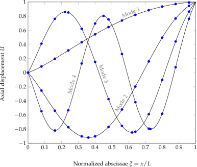
Figure 6: First four eigenfunctions for axial vibrations of the cantilever beam in Fig. 5: Proposed approach (continuous line), Rayleigh-Ritz method (dots).

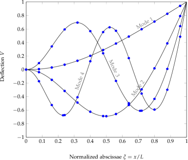
Figure 7: First four eigenfunctions for bending vibrations of the cantilever beam in Fig. 5: Proposed approach (continuous line), Rayleigh-Ritz method (dots).

5.2 Example B

Consider the small-size 2D structures in Fig. 8. The two structures feature the same external constraints but two different assumptions are made on the internal nodes, i.e. truss (Fig. 8a) and frame (Fig. 8b) nodal connections are considered. For numerical purposes, reference parameters are: $E=427\hskip 1.5pt\text{GPa}$, $L=20\hskip 1.5pt\text{nm}$, $A=2\hskip 1.5pt\text{$\text{nm}^{2}$}$ (rectangular cross section with $b=1\hskip 1.5pt\text{nm}$ and $h=2\hskip 1.5pt\text{nm}$), $\rho=3200\hskip 1.5pt\text{kg$\text{m}^{-3}$}$.

Figure 8: Small-size 2D structures: (a) truss; (b) frame.

To investigate the free-vibration response in presence of size effects, every structural member is modelled by a single stress-driven nonlocal two-node beam element, whose exact dynamic stiffness matrix is $\mathbf{D}$ given by Eq. (26) for the frame or its block matrix $\mathbf{D}_{a}$ for the truss. On building the global dynamic stiffness matrix by a standard finite-element assembly procedure, exact natural frequencies and modes are calculated by the WW algorithm described in Section 4. Size effects are investigated considering different values of the internal length $\lambda$ of the stress-driven nonlocal model.

Table 4: Natural frequencies, $J_{0}$ and $s[\mathbf{D}_{G}]$ for truss in Fig. 8a.

$\lambda$	0			0.01			0.10
	$\omega~{}(\hskip 1.5pt\text{GHz})$	$J_{0}$	$s[\mathbf{D}_{G}]$	$\omega~{}(\hskip 1.5pt\text{GHz})$	$J_{0}$	$s[\mathbf{D}_{G}]$	$\omega~{}(\hskip 1.5pt\text{GHz})$	$J_{0}$	$s[\mathbf{D}_{G}]$
	27.43821	0	1	27.57524	0	1	28.92544	0	1
	58.27909	0	2	58.56994	0	2	61.51358	0	2
	63.87465	0	4	64.20284	0	4	67.53415	0	4
	63.87465	0	4	64.20284	0	4	67.53415	0	4
	72.19697	0	5	72.56269	0	5	76.27531	0	5
	75.49053	0	6	75.86652	0	6	79.78619	0	6
	89.90719	0	7	90.34393	0	7	94.99763	0	7
	101.00278	0	9	101.47942	0	9	106.72088	0	9
	101.00278	0	9	101.47942	0	9	106.72088	0	9
	130.70334	0	10	131.39556	0	10	139.26081	0	10
	144.39394	0	11	145.13719	0	11	153.55326	0	11
	161.97629	0	13	162.98630	0	13	174.80492	0	13
	161.97629	0	13	162.98630	0	13	174.80492	0	13
	170.78182	0	14	171.94402	0	14	185.74609	0	14
	176.32509	0	15	177.47886	0	15	191.44679	0	15
	184.61555	0	17	185.96370	0	17	202.32571	0	17
	184.61555	0	17	185.96370	0	17	202.32571	0	17
	191.85137	0	18	193.44083	0	18	212.98799	0	18
	209.44418	8	11	211.20072	8	11	232.47553	0	19
	216.59091	8	12	217.73242	8	12	234.52643	0	20

For a first insight, the truss model in Fig. 8a is considered. Table 4 shows the first 20 natural frequencies computed by the proposed approach, along with the numbers $J_{0}$ and $s[\mathbf{D}_{G}]$ corresponding to each natural frequency calculated by the WW algorithm. Results in Table 4 suggest some interesting comments. The first is that the natural frequencies increase with the internal length $\lambda$, meaning that increasing nonlocality induces stiffening. This is in agreement with previous results obtained for the static response using the stress-driven nonlocal approach (Romano and Barretta, 2017a, b; Romano et al., 2017); as for size effects in general, it is to be noticed that experimental evidence of stiffening size effects exists in the literature for small-size specimens, see for instance the work by Lam et al. (2003). A second observation is that the natural frequencies tend to those of the classical local model as the internal length $\lambda$ decreases, as expected.

Finally, it is noteworthy that some of the natural frequencies reported in Table 4 are double roots of the characteristic equation, confirming that the WW algorithm is capable of detecting all natural frequencies, including multiple ones. The mode shapes associated with some of the natural frequencies in Table 4 are illustrated in Fig. 9.

(a) $1^{\mathrm{st}}$ mode

(b) $2^{\mathrm{nd}}$ mode

(c) $5^{\mathrm{th}}$ mode

(d) $6^{\mathrm{th}}$ mode

Figure 9: Mode shapes for truss in Fig. 8a, for $\lambda=0.10$.

They appear meaningful based on engineering judgement and exhibit typical symmetric or anti-symmetric shapes, as is typical the case in vibrating structures.

Next, the frame in Fig. 8b is investigated. Table 5 reports the first 20 natural frequencies obtained by the proposed approach along with the pertinent numbers $J_{0}$ and $s[\mathbf{D}_{G}]$. Comments mirrors those on Table 4. That is, the natural frequencies increase with the internal length $\lambda$, i.e. increasing nonlocality induces stiffening effects in the free-vibration response, while the local natural frequencies are retrieved for vanishing $\lambda$. For a final insight, Fig. 11 illustrates the frequency response for the horizontal displacement of the top-right node, when a harmonic horizontal force $1e^{i\omega t}$ (expressed in  nN) is applied at the same node of the frame. As expected, the resonance peaks of the frequency response occur at the natural frequencies reported in Table 5 for various internal lengths $\lambda$’s. The results in Fig. 11 substantiate the correctness of the proposed approach.

Table 5: Natural frequencies, $J_{0}$ and $s[\mathbf{D}_{G}]$ for frame in Fig. 8b.

$\lambda$	0			0.01			0.10
	$\omega~{}(\hskip 1.5pt\text{GHz})$	$J_{0}$	$s[\mathbf{D}_{G}]$	$\omega~{}(\hskip 1.5pt\text{GHz})$	$J_{0}$	$s[\mathbf{D}_{G}]$	$\omega~{}(\hskip 1.5pt\text{GHz})$	$J_{0}$	$s[\mathbf{D}_{G}]$
	18.06966	0	1	18.20830	0	1	19.74251	0	1
	21.43257	0	2	21.66017	0	2	24.85028	0	2
	21.82279	0	3	22.07537	0	3	25.64302	0	3
	24.23064	0	4	24.55413	0	4	28.90690	0	4
	24.64898	0	5	24.99159	0	5	29.58275	0	5
	25.11337	0	6	25.48482	0	6	30.54844	0	6
	26.38111	0	7	26.75646	0	7	31.37600	0	7
	27.73741	0	8	28.01785	0	8	32.04594	0	8
	29.36164	0	9	29.97324	0	9	33.37855	0	9
	30.50700	8	2	30.63232	8	2	37.90881	0	10
	33.07618	8	3	33.39250	8	3	39.42049	0	11
	36.73234	8	4	37.08584	8	4	42.08654	8	4
	36.90634	8	5	37.29529	8	5	42.64020	8	5
	37.22135	8	6	37.67109	8	6	44.91988	8	6
	39.65386	8	7	40.09235	8	7	46.64787	8	7
	40.83422	8	8	41.28685	8	8	48.15536	8	8
	41.20524	8	9	41.74052	8	9	49.12239	8	9
	42.17990	8	10	42.71746	8	10	49.56440	8	10
	44.39416	8	11	44.97509	8	11	52.63650	8	11
	45.49144	8	12	46.10350	8	12	54.30830	8	12

Mode shapes associated with some of the natural frequencies in Table 5, reported in Fig. 10, exhibit symmetry and anti-symmetry as expected in vibrating structures.

(a) $1^{\mathrm{st}}$ mode

(b) $2^{\mathrm{nd}}$ mode

(c) $3^{\mathrm{rd}}$ mode

(d) $5^{\mathrm{th}}$ mode

Figure 10: Mode shapes for frame in Fig. 8b, for $\lambda=0.10$.

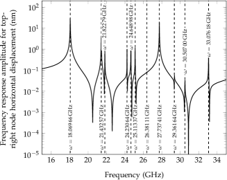
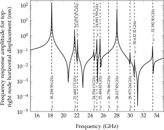
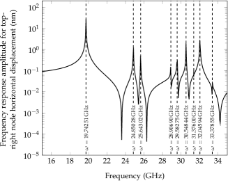
Figure 11: Frequency response function for horizontal displacement of top-right node of frame in Fig. 8b, for various internal lengths: (a) $\lambda=0$, (b) $\lambda=0.01$, (c) $\lambda=0.10$.

6 Closing remarks

A novel approach to the dynamics of small-size frames has been proposed, resorting to the analysis presented in (Romano and Barretta, 2017a) within special framework of straight beams. On adopting a stress-driven nonlocal formulation to account for size effects, the exact dynamic stiffness matrix of a two-node nonlocal element has been analytically derived in a closed form, which can readily be used to construct, by a standard finite-element assembly procedure, the global dynamic stiffness matrix of complex small-size frames. The Wittrick-Williams algorithm has been applied to calculate all natural frequencies and related modes. The formulation has been presented for 2D structures, but can be generalized to 3D ones.

The proposed approach provides, to the best of authors’ knowledge, a first example of two-node nonlocal element, whose dynamics is treated exactly using the dynamic-stiffness matrix approach. That is, every member of the frame can be modelled by a single, exact element without any internal mesh. The stress-driven approach offers a consistent nonlocal description of size effects that does overcome theoretical flaws of alternative nonlocal formulations. Finally, using the Wittrick-Williams technique guarantees that all natural frequencies can be calculated without missing anyone and including multiple ones. It is believed that the proposed methodology provides an effective and robust tool to assess scale effects in nano-frames, within the general framework of nonlocal mechanics.

Appendix A

This Appendix reports closed analytical expressions of functions $f_{k}$ and $g_{k}$ involved in Eq. (20) and Eq. (21) of the main text. First, notice that the solution of the $4^{\mathrm{th}}$ order differential equation (16) takes the general expression:

$$U(\xi)=\sum_{k=1}^{2}c_{a,k}\mathrm{e}^{\sqrt{r_{k}}\xi}+c_{a,k+2}\mathrm{e}^{-\sqrt{r_{k}}\xi}$$ (66)

where $c_{a,k}$ (for $k=1,...,4$) are integration constants and $\pm\sqrt{r_{k}}$ (for $k=1,...,2$) are the roots of the characteristic polynomial of Eq. (16), obtained in the following form on assuming the solution $U=\mathrm{e}^{y\xi}$ and setting $y^{2}=r$:

$$-\lambda^{2}r^{2}+r+\overline{\omega}_{a}^{2}=0$$ (67)

Enforcing the constitutive BCs (17a,b), (66) reverts to Eq. (20) where functions $f_{k}$ are:

$$f_{1}(\xi)=\mathcal{A}_{1}\mathrm{e}^{-r_{1}\xi}+\mathcal{A}_{2}\mathrm{e}^{-r_{2}\xi}+\mathrm{e}^{r_{1}\xi}$$ (68)

$$f_{2}(\xi)=\mathcal{A}_{3}\mathrm{e}^{-r_{1}\xi}+\mathcal{A}_{4}\mathrm{e}^{-r_{2}\xi}+\mathrm{e}^{r_{2}\xi}$$

In Eq. (68), symbols $A_{k}$ (for $k=1,...,4$) and $r_{k}$ (for $k=1,2$)

$$\mathcal{A}_{1}=\mathcal{O}_{1}^{-1}\mathrm{e}^{r_{1}}\left(\lambda^{2}\mathrm{e}^{r_{1}+r_{2}}r_{1}r_{2}-\lambda^{2}r_{1}r_{2}+\lambda\mathrm{e}^{r_{1}+r_{2}}r_{1}+\lambda r_{1}+\lambda\mathrm{e}^{r_{1}+r_{2}}r_{2}+\lambda r_{2}+\mathrm{e}^{r_{1}+r_{2}}-1\right)$$ (69)

$$\mathcal{A}_{2}=-(r_{2}\mathcal{O}_{1})^{-1}\mathrm{e}^{r_{2}}r_{1}\left(\lambda^{2}\mathrm{e}^{2r_{1}}r_{1}^{2}-\lambda^{2}r_{1}^{2}+2\lambda\mathrm{e}^{2r_{1}}r_{1}+2\lambda r_{1}+\mathrm{e}^{2r_{1}}-1\right)$$

$$\mathcal{A}_{3}=(r_{1}\mathcal{O}_{1})^{-1}\mathrm{e}^{r_{1}}r_{2}\left(\lambda^{2}\mathrm{e}^{2r_{2}}r_{2}^{2}-\lambda^{2}r_{2}^{2}+2\lambda\mathrm{e}^{2r_{2}}r_{2}+2\lambda r_{2}+\mathrm{e}^{2r_{2}}-1\right)$$

$$\mathcal{A}_{4}=-\mathcal{O}_{1}^{-1}\mathrm{e}^{r_{2}}\left(\lambda^{2}\mathrm{e}^{r_{1}+r_{2}}r_{1}r_{2}-\lambda^{2}r_{1}r_{2}+\lambda\mathrm{e}^{r_{1}+r_{2}}r_{1}+\lambda r_{1}+\lambda\mathrm{e}^{r_{1}+r_{2}}r_{2}+\lambda r_{2}+\mathrm{e}^{r_{1}+r_{2}}-1\right)$$

with

$$\mathcal{O}_{1}=\lambda^{2}\mathrm{e}^{p_{1}}p_{1}p_{2}-\lambda^{2}\mathrm{e}^{p_{2}}p_{1}p_{2}-\lambda\mathrm{e}^{p_{1}}p_{1}-\lambda\mathrm{e}^{p_{2}}p_{1}+\lambda\mathrm{e}^{p_{1}}p_{2}+\lambda\mathrm{e}^{p_{2}}p_{2}-\mathrm{e}^{p_{1}}+\mathrm{e}^{p_{2}}$$ (70)

Further, recognize that the solution of the $6^{\mathrm{th}}$ order differential equation (18) takes the general expression (e.g., see Pinnola et al. (2020b)):

$$V(\xi)=\sum_{k=1}^{3}c_{b,k}\mathrm{e}^{\sqrt{p_{k}}\xi}+c_{b,k+3}\mathrm{e}^{-\sqrt{p_{k}}\xi}$$ (71)

where $c_{b,k}$ (for $k=1,...,6$) are integration constants and $\pm\sqrt{p_{k}}$ (for $k=1,...,3$) are the roots of the characteristic polynomial of Eq. (18), obtained in the following form on assuming the solution $V=\mathrm{e}^{y\xi}$ and setting $y^{2}=p$:

$$\lambda^{2}p^{3}-p^{2}+\overline{\omega}_{b}^{4}=0$$ (72)

Enforcing the constitutive BCs (19a,b), (71) becomes Eq. (21) where functions $g_{k}$ are:

$$g_{1}(\xi)=\mathrm{e}^{p_{1}\xi}+\mathcal{B}_{1}\mathrm{e}^{-p_{2}\xi}+\mathcal{B}_{2}\mathrm{e}^{-p_{3}\xi}$$ (73)

$$g_{2}(\xi)=\mathrm{e}^{p_{2}\xi}+\mathcal{B}_{3}\mathrm{e}^{-p_{2}\xi}+\mathcal{B}_{4}\mathrm{e}^{-p_{3}\xi}$$

$$g_{3}(\xi)=\mathrm{e}^{p_{3}\xi}+\mathcal{B}_{5}\mathrm{e}^{-p_{2}\xi}+\mathcal{B}_{6}\mathrm{e}^{-p_{3}\xi}$$

$$g_{4}(\xi)=\mathrm{e}^{-p_{1}\xi}+\mathcal{B}_{7}\mathrm{e}^{-p_{2}\xi}+\mathcal{B}_{8}\mathrm{e}^{-p_{3}\xi}$$

In Eq. (73), symbols $\mathcal{B}_{k}$ (for $k=1,...,8$) and $p_{k}$ (for $k=1,...,3$) denote:

$$\mathcal{B}_{1}=-(p_{2}^{2}\mathcal{O}_{2})^{-1}\mathrm{e}^{p_{2}}p_{1}^{2}\left(\mathrm{e}^{p_{1}+p_{3}}p_{1}p_{3}\lambda^{2}-p_{1}p_{3}\lambda^{2}+\mathrm{e}^{p_{1}+p_{3}}p_{1}\lambda+p_{1}\lambda+\mathrm{e}^{p_{1}+p_{3}}p_{3}\lambda+p_{3}\lambda+\mathrm{e}^{p_{1}+p_{3}}-1\right)$$ (74)

$$\mathcal{B}_{2}=(p_{3}^{2}\mathcal{O}_{2})^{-1}\mathrm{e}^{p_{3}}p_{1}^{2}\left(\mathrm{e}^{p_{1}+p_{2}}p_{1}p_{2}\lambda^{2}-p_{1}p_{2}\lambda^{2}+\mathrm{e}^{p_{1}+p_{2}}p_{1}\lambda+p_{1}\lambda+\mathrm{e}^{p_{1}+p_{2}}p_{2}\lambda+p_{2}\lambda+\mathrm{e}^{p_{1}+p_{2}}-1\right)$$

$$\mathcal{B}_{3}=-\mathcal{O}_{2}^{-1}\mathrm{e}^{p_{2}}\left(\mathrm{e}^{p_{2}+p_{3}}p_{2}p_{3}\lambda^{2}-p_{2}p_{3}\lambda^{2}+\mathrm{e}^{p_{2}+p_{3}}p_{2}\lambda+p_{2}\lambda+\mathrm{e}^{p_{2}+p_{3}}p_{3}\lambda+p_{3}\lambda+\mathrm{e}^{p_{2}+p_{3}}-1\right)$$

$$\mathcal{B}_{4}=(p_{3}^{2}\mathcal{O}_{2})^{-1}\mathrm{e}^{p_{3}}p_{2}^{2}\left(\mathrm{e}^{2p_{2}}\lambda^{2}p_{2}^{2}-\lambda^{2}p_{2}^{2}+2\mathrm{e}^{2p_{2}}\lambda p_{2}+2\lambda p_{2}+\mathrm{e}^{2p_{2}}-1\right)$$

$$\mathcal{B}_{5}=-(p_{2}^{2}\mathcal{O}_{2})^{-1}\mathrm{e}^{p_{2}}p_{3}^{2}\left(\mathrm{e}^{2p_{3}}\lambda^{2}p_{3}^{2}-\lambda^{2}p_{3}^{2}+2\mathrm{e}^{2p_{3}}\lambda p_{3}+2\lambda p_{3}+\mathrm{e}^{2p_{3}}-1\right)$$

$$\mathcal{B}_{6}=\mathcal{O}_{2}^{-1}\mathrm{e}^{p_{3}}\left(\mathrm{e}^{p_{2}+p_{3}}p_{2}p_{3}\lambda^{2}-p_{2}p_{3}\lambda^{2}+\mathrm{e}^{p_{2}+p_{3}}p_{2}\lambda+p_{2}\lambda+\mathrm{e}^{p_{2}+p_{3}}p_{3}\lambda+p_{3}\lambda+\mathrm{e}^{p_{2}+p_{3}}-1\right)$$

$$\mathcal{B}_{7}=-(p_{2}^{2}\mathcal{O}_{2})^{-1}\mathrm{e}^{p_{2}-p_{1}}p_{1}^{2}\left(\mathrm{e}^{p_{1}}p_{1}p_{3}\lambda^{2}-\mathrm{e}^{p_{3}}p_{1}p_{3}\lambda^{2}-\mathrm{e}^{p_{1}}p_{1}\lambda-\mathrm{e}^{p_{3}}p_{1}\lambda+\mathrm{e}^{p_{1}}p_{3}\lambda+\mathrm{e}^{p_{3}}p_{3}\lambda-\mathrm{e}^{p_{1}}+\mathrm{e}^{p_{3}}\right)$$

$$\mathcal{B}_{8}=(p_{3}^{2}\mathcal{O}_{2})^{-1}\mathrm{e}^{p_{3}-p_{1}}p_{1}^{2}\left(\mathrm{e}^{p_{1}}p_{1}p_{2}\lambda^{2}-\mathrm{e}^{p_{2}}p_{1}p_{2}\lambda^{2}-\mathrm{e}^{p_{1}}p_{1}\lambda-\mathrm{e}^{p_{2}}p_{1}\lambda+\mathrm{e}^{p_{1}}p_{2}\lambda+\mathrm{e}^{p_{2}}p_{2}\lambda-\mathrm{e}^{p_{1}}+\mathrm{e}^{p_{2}}\right)$$

being

$$\mathcal{O}_{2}=\mathrm{e}^{p_{2}}p_{2}p_{3}\lambda^{2}-\mathrm{e}^{p_{3}}p_{2}p_{3}\lambda^{2}-\mathrm{e}^{p_{2}}p_{2}\lambda-\mathrm{e}^{p_{3}}p_{2}\lambda+\mathrm{e}^{p_{2}}p_{3}\lambda+\mathrm{e}^{p_{3}}p_{3}\lambda-\mathrm{e}^{p_{2}}+\mathrm{e}^{p_{3}}$$ (75)

Appendix B

This Appendix describes the formulation of the eigenvalue problem for the free vibrations of stress-driven nonlocal beams, according to the Rayleigh-Ritz method (Meirovitch, 1997) using Chebyshëv polynomials (Mason and Handscomb, 2002) as trial functions.

For axial vibrations, the Rayleigh’s quotient is defined by

$$\overline{\omega}_{a}^{2}=R(U)=\frac{\int_{0}^{1}\left(\lambda^{2}\frac{{\mathrm{d}^{4}U}}{\mathrm{d}\xi^{4}}U-\frac{{\mathrm{d}^{2}U}}{\mathrm{d}\xi^{2}}\right)~{}\mathrm{d}\xi}{\int_{0}^{1}U^{2}~{}\mathrm{d}\xi}$$ (76)

where $U$ is an eigenfunction. Next, integrate by parts the numerator of Eq. (76), enforce the constitutive BCs (17a,b) along with the static BCs and assume that $U(\xi)$ is written as an expansion of $N$ shifted Chebyshëv polynomials of the first kind:

$$U(\xi)=\mathbf{c}^{\mathrm{T}}\boldsymbol{\phi}(\xi)$$ (77)

where $\mathbf{c}=\begin{bmatrix}c_{0}&\dots&c_{N}\end{bmatrix}^{\mathrm{T}}$ is the vector of constants and $\boldsymbol{\phi}(\xi)$ is the vector

$$\boldsymbol{\phi}(\xi)=\begin{bmatrix}T_{0}(-1+2\xi)&\dots&T_{N}(-1+2\xi)\end{bmatrix}^{\mathrm{T}}$$ (78)

being $T_{j}$ the $j^{\mathrm{th}}$ Chebyshëv polynomial defined by the following recurrence relation (Mason and Handscomb, 2002):

$$T_{j}(x)=2xT_{j-1}(x)-T_{j-2}(x),\qquad j=2,3,...$$ (79)

with $T_{0}(x)=1$ and $T_{1}(x)=x$. Using Eq. (77), the stationary condition of the Rayleigh’s quotient implies that

$$\frac{\partial R(\mathbf{c})}{\partial\mathbf{c}}=\mathbf{0}$$ (80)

Eq. (80) leads to following generalized eigenproblem:

$$\left(\mathbf{A}_{a}-\overline{\omega}_{a}^{2}\mathbf{B}\right)\mathbf{c}=\mathbf{0}$$ (81)

where

$$\mathbf{A}_{a}=\int_{0}^{1}\left(\lambda^{2}\frac{{\mathrm{d}^{2}\boldsymbol{\phi}}}{\mathrm{d}\xi^{2}}\otimes\frac{{\mathrm{d}^{2}\boldsymbol{\phi}}}{\mathrm{d}\xi^{2}}+\frac{\mathrm{d}\boldsymbol{\phi}}{\mathrm{d}\xi}\otimes\frac{\mathrm{d}\boldsymbol{\phi}}{\mathrm{d}\xi}\right)~{}\mathrm{d}\xi+\lambda\left(\left.\frac{\mathrm{d}\boldsymbol{\phi}}{\mathrm{d}\xi}\otimes\frac{\mathrm{d}\boldsymbol{\phi}}{\mathrm{d}\xi}\right\rvert_{\xi=0}+\left.\frac{\mathrm{d}\boldsymbol{\phi}}{\mathrm{d}\xi}\otimes\frac{\mathrm{d}\boldsymbol{\phi}}{\mathrm{d}\xi}\right\rvert_{\xi=1}\right)$$ (82)

and

$$\mathbf{B}=\int_{0}^{1}\boldsymbol{\phi}\otimes\boldsymbol{\phi}~{}\mathrm{d}\xi$$ (83)

In a similar fashion, the generalized eigenproblem is derived for bending responses. In this case, the Rayleigh’s quotient is defined by

$$\overline{\omega}_{b}^{4}=R(V)=\frac{\int_{0}^{1}\left(-\lambda^{2}\frac{{\mathrm{d}^{6}V}}{\mathrm{d}\xi^{6}}V+\frac{{\mathrm{d}^{5}V}}{\mathrm{d}\xi^{5}}V\right)~{}\mathrm{d}\xi}{\int_{0}^{1}V^{2}~{}\mathrm{d}\xi}$$ (84)

with $V$ an eigenfunction. Again, the numerator of Eq. (76) is integrated by part, the constitutive BCs (19a,b) along with static BCs are enforced and $V(\xi)$ is written as an expansion of $N$ shifted Chebyshëv polynomials of the first kind:

$$V(\xi)=\mathbf{c}^{\mathrm{T}}\boldsymbol{\phi}(\xi)$$ (85)

where $\mathbf{c}=\begin{bmatrix}c_{0}&\dots&c_{N}\end{bmatrix}^{\mathrm{T}}$ is the vector of constants and $\boldsymbol{\phi}(\xi)$ is the vector (78). Finally, replacing (84) for $R$ in Eq. (80) leads to the following eigenproblem

$$\left(\mathbf{A}_{b}-\overline{\omega}_{b}^{4}\mathbf{B}\right)\mathbf{c}=\mathbf{0}$$ (86)

where

$$\mathbf{A}_{b}=\int_{0}^{1}\left(\lambda^{2}\frac{{\mathrm{d}^{3}\boldsymbol{\phi}}}{\mathrm{d}\xi^{3}}\otimes\frac{{\mathrm{d}^{3}\boldsymbol{\phi}}}{\mathrm{d}\xi^{3}}+\frac{{\mathrm{d}^{2}\boldsymbol{\phi}}}{\mathrm{d}\xi^{2}}\otimes\frac{{\mathrm{d}^{2}\boldsymbol{\phi}}}{\mathrm{d}\xi^{2}}\right)~{}\mathrm{d}\xi+\lambda\left(\left.\frac{{\mathrm{d}^{2}\boldsymbol{\phi}}}{\mathrm{d}\xi^{2}}\otimes\frac{{\mathrm{d}^{2}\boldsymbol{\phi}}}{\mathrm{d}\xi^{2}}\right\rvert_{\xi=0}+\left.\frac{{\mathrm{d}^{2}\boldsymbol{\phi}}}{\mathrm{d}\xi^{2}}\otimes\frac{{\mathrm{d}^{2}\boldsymbol{\phi}}}{\mathrm{d}\xi^{2}}\right\rvert_{\xi=1}\right)$$ (87)

and $\mathbf{B}$ is given by Eq. (83). It has to be noticed that, in the formulation of both eigenvalue problems (81) and (86), kinematic BCs can be suitably enforced on the trial functions using the method of Lagrange multipliers (Canales and Mantari, 2016). This leads to the following eigenvalue problems:

$$\left(\begin{bmatrix}\mathbf{A}_{a}&\mathbf{L}_{a}\\ \mathbf{L}_{a}^{\mathrm{T}}&\mathbf{0}\end{bmatrix}-\overline{\omega}_{a}^{2}\begin{bmatrix}\mathbf{B}&\mathbf{0}\\ \mathbf{0}&\mathbf{0}\end{bmatrix}\right)\begin{bmatrix}\mathbf{c}\\ \boldsymbol{\mu}\end{bmatrix}=\mathbf{0}\qquad\left(\begin{bmatrix}\mathbf{A}_{b}&\mathbf{L}_{b}\\ \mathbf{L}_{b}^{\mathrm{T}}&\mathbf{0}\end{bmatrix}-\overline{\omega}_{b}^{4}\begin{bmatrix}\mathbf{B}&\mathbf{0}\\ \mathbf{0}&\mathbf{0}\end{bmatrix}\right)\begin{bmatrix}\mathbf{c}\\ \boldsymbol{\mu}\end{bmatrix}=\mathbf{0}$$ (87a,b)

with $\mathbf{L}_{a}$ and $\mathbf{L}_{b}$ involving the trial functions computed at beam ends according to kinematic BCs. For instance, for a cantilever beam:

$$\mathbf{L}_{a}=\begin{bmatrix}\boldsymbol{\phi}(0)\end{bmatrix}\qquad\mathbf{L}_{b}=\begin{bmatrix}\boldsymbol{\phi}(0)&\left.\frac{\mathrm{d}\boldsymbol{\phi}}{\mathrm{d}\xi}\right\rvert_{\xi=0}\end{bmatrix}$$ (88a,b)

Acknowledgment - Financial supports from MIUR in the framework of the Project PRIN 2017 - code 2017J4EAYB Multiscale Innovative Materials and Structures (MIMS) - University of Naples Federico II Research Unit is gratefully acknowledged.

References

- Aifantis (1999) Aifantis, E., 1999. Gradient deformation models at nano, micro, and macro scales. Journal of Engineering Materials and Technology, Transactions of the ASME 121, 189–202.
- Aifantis (2003) Aifantis, E.C., 2003. Update on a class of gradient theories. Mechanics of materials 35, 259–280.
- Aifantis (2009) Aifantis, E.C., 2009. Exploring the applicability of gradient elasticity to certain micro/nano reliability problems. Microsystem Technologies 15, 109–115.
- Aifantis (2011) Aifantis, E.C., 2011. On the gradient approach–relation to eringen’s nonlocal theory. International Journal of Engineering Science 49, 1367–1377.
- Akgöz and Civalek (2013) Akgöz, B., Civalek, Ö., 2013. A size-dependent shear deformation beam model based on the strain gradient elasticity theory. International Journal of Engineering Science 70, 1–14.
- Alotta et al. (2017a) Alotta, G., Failla, G., Pinnola, F., 2017a. Stochastic analysis of a nonlocal fractional viscoelastic bar forced by gaussian white noise. ASCE-ASME Journal of Risk and Uncertainty in Engineering Systems, Part B: Mechanical Engineering 3.
- Alotta et al. (2014) Alotta, G., Failla, G., Zingales, M., 2014. Finite element method for a nonlocal timoshenko beam model. Finite Elements in Analysis and Design 89, 77–92.
- Alotta et al. (2017b) Alotta, G., Failla, G., Zingales, M., 2017b. Finite-element formulation of a nonlocal hereditary fractional-order timoshenko beam. Journal of Engineering Mechanics 143, D4015001.
- Aria and Friswell (2019) Aria, A., Friswell, M., 2019. A nonlocal finite element model for buckling and vibration of functionally graded nanobeams. Composites Part B: Engineering 166, 233–246.
- Askes and Aifantis (2011) Askes, H., Aifantis, E.C., 2011. Gradient elasticity in statics and dynamics: an overview of formulations, length scale identification procedures, finite element implementations and new results. International Journal of Solids and Structures 48, 1962–1990.
- Attia and Abdel Rahman (2018) Attia, M.A., Abdel Rahman, A.A., 2018. On vibrations of functionally graded viscoelastic nanobeams with surface effects. International Journal of Engineering Science 127, 1 – 32.
- Banerjee (1997) Banerjee, J., 1997. Dynamic stiffness formulation for structural elements: a general approach. Computers & structures 63, 101–103.
- Banerjee (1998) Banerjee, J., 1998. Free vibration of axially loaded composite timoshenko beams using the dynamic stiffness matrix method. Computers & Structures 69, 197 – 208.
- Banerjee (2001) Banerjee, J., 2001. Frequency equation and mode shape formulae for composite timoshenko beams. Composite Structures 51, 381 – 388.
- Banerjee and Williams (1985) Banerjee, J., Williams, F., 1985. Exact bernoulli–euler dynamic stiffness matrix for a range of tapered beams. International Journal for Numerical Methods in Engineering 21, 2289–2302.
- Banerjee and Williams (1992) Banerjee, J., Williams, F., 1992. Coupled bending-torsional dynamic stiffness matrix for timoshenko beam elements. Computers & Structures 42, 301–310.
- Banerjee and Williams (1996) Banerjee, J., Williams, F., 1996. Exact dynamic stiffness matrix for composite timoshenko beams with applications. Journal of Sound and Vibration 194, 573 – 585.
- Banerjee (2003) Banerjee, J.R., 2003. Dynamic Stiffness Formulation and Its Application for a Combined Beam and a Two Degree-of-Freedom System . Journal of Vibration and Acoustics 125, 351–358.
- Barretta et al. (2017) Barretta, R., Brčić, M., Čanađija, M., Luciano, R., Marotti de Sciarra, F., 2017. Application of gradient elasticity to armchair carbon nanotubes: Size effects and constitutive parameters assessment. European Journal of Mechanics - A/Solids 65, 1 – 13.
- Barretta et al. (2019a) Barretta, R., Faghidian, S.A., Luciano, R., 2019a. Longitudinal vibrations of nano-rods by stress-driven integral elasticity. Mechanics of Advanced Materials and Structures 26, 1307–1315.
- Barretta et al. (2018) Barretta, R., Faghidian, S.A., Luciano, R., Medaglia, C., Penna, R., 2018. Stress-driven two-phase integral elasticity for torsion of nano-beams. Composites Part B: Engineering 145, 62–69.
- Barretta et al. (2019b) Barretta, R., Faghidian, S.A., Marotti de Sciarra, F., 2019b. Stress-driven nonlocal integral elasticity for axisymmetric nano-plates. International Journal of Engineering Science 136, 38 – 52.
- Bi et al. (2020) Bi, L., Yin, J., Huang, X., Wang, Y., Yang, Z., 2020. Graphene pillared with hybrid fullerene and nanotube as a novel 3d framework for hydrogen storage: A dft and gcmc study. International Journal of Hydrogen Energy 45, 17637 – 17648.
- Canales and Mantari (2016) Canales, F., Mantari, J., 2016. Buckling and free vibration of laminated beams with arbitrary boundary conditions using a refined hsdt. Composites Part B: Engineering 100, 136 – 145.
- Challamel (2018) Challamel, N., 2018. Static and dynamic behaviour of nonlocal elastic bar using integral strain-based and peridynamic models. Comptes Rendus Mécanique 346, 320–335.
- Challamel et al. (2016) Challamel, N., Wang, C., Elishakoff, I., 2016. Nonlocal or gradient elasticity macroscopic models: a question of concentrated or distributed microstructure. Mechanics Research Communications 71, 25–31.
- Challamel and Wang (2008) Challamel, N., Wang, C.M., 2008. The small length scale effect for a non-local cantilever beam: a paradox solved. Nanotechnology 19, 345703.
- Chao et al. (2020) Chao, M., Wang, Y., Ma, D., Wu, X., Zhang, W., Zhang, L., Wan, P., 2020. Wearable mxene nanocomposites-based strain sensor with tile-like stacked hierarchical microstructure for broad-range ultrasensitive sensing. Nano Energy 78, 105187.
- Courant and Hilbert (1953) Courant, R., Hilbert, D., 1953. Methods of Mathematical Physics. Interscience Publishers.
- Darban et al. (2020) Darban, H., Luciano, R., Caporale, A., Fabbrocino, F., 2020. Higher modes of buckling in shear deformable nanobeams. International Journal of Engineering Science 154, 103338.
- Dastjerdi and Akgöz (2019) Dastjerdi, S., Akgöz, B., 2019. On the statics of fullerene structures. International Journal of Engineering Science 142, 125 – 144.
- Demir and Civalek (2017) Demir, Ç., Civalek, Ö., 2017. On the analysis of microbeams. International Journal of Engineering Science 121, 14–33.
- Di Paola et al. (2009) Di Paola, M., Failla, G., Zingales, M., 2009. Physically-based approach to the mechanics of strong non-local linear elasticity theory. Journal of Elasticity 97, 103–130.
- Di Paola et al. (2010) Di Paola, M., Failla, G., Zingales, M., 2010. The mechanically-based approach to 3d non-local linear elasticity theory: Long-range central interactions. International Journal of Solids and Structures 47, 2347 – 2358.
- Di Paola et al. (2013) Di Paola, M., Failla, G., Zingales, M., 2013. Non-local stiffness and damping models for shear-deformable beams. European Journal of Mechanics-A/Solids 40, 69–83.
- Eringen (1983) Eringen, A., 1983. On differential equations of nonlocal elasticity and solutions of screw dislocation and surface waves. Journal of Applied Physics 54, 4703–4710.
- Eringen (1972) Eringen, A.C., 1972. Linear theory of nonlocal elasticity and dispersion of plane waves. International Journal of Engineering Science 10, 425–435.
- Failla (2016) Failla, G., 2016. An exact generalised function approach to frequency response analysis of beams and plane frames with the inclusion of viscoelastic damping. Journal of Sound and Vibration 360, 171 – 202.
- Farajpour et al. (2018) Farajpour, A., Ghayesh, M.H., Farokhi, H., 2018. A review on the mechanics of nanostructures. International Journal of Engineering Science 133, 231 – 263.
- Farajpour et al. (2020) Farajpour, A., Howard, C.Q., Robertson, W.S., 2020. On size-dependent mechanics of nanoplates. International Journal of Engineering Science 156, 103368.
- Fasano et al. (2015) Fasano, M., Bozorg Bigdeli, M., Vaziri Sereshk, M.R., Chiavazzo, E., Asinari, P., 2015. Thermal transmittance of carbon nanotube networks: Guidelines for novel thermal storage systems and polymeric material of thermal interest. Renewable and Sustainable Energy Reviews 41, 1028 – 1036.
- Fernández-Sáez et al. (2016) Fernández-Sáez, J., Zaera, R., Loya, J., Reddy, J., 2016. Bending of euler–bernoulli beams using eringen’s integral formulation: a paradox resolved. International Journal of Engineering Science 99, 107–116.
- Fuschi et al. (2019) Fuschi, P., Pisano, A., Polizzotto, C., 2019. Size effects of small-scale beams in bending addressed with a strain-difference based nonlocal elasticity theory. International Journal of Mechanical Sciences 151, 661–671.
- Genoese et al. (2017) Genoese, A., Genoese, A., Rizzi, N.L., Salerno, G., 2017. On the derivation of the elastic properties of lattice nanostructures: The case of graphene sheets. Composites Part B: Engineering 115, 316 – 329.
- Ghayesh and Farajpour (2019) Ghayesh, M.H., Farajpour, A., 2019. A review on the mechanics of functionally graded nanoscale and microscale structures. International Journal of Engineering Science 137, 8 – 36.
- Ghayesh et al. (2019) Ghayesh, M.H., Farajpour, A., Farokhi, H., 2019. Viscoelastically coupled mechanics of fluid-conveying microtubes. International Journal of Engineering Science 145, 103139.
- Gholipour and Ghayesh (2020) Gholipour, A., Ghayesh, M.H., 2020. Nonlinear coupled mechanics of functionally graded nanobeams. International Journal of Engineering Science 150, 103221.
- Hozhabrossadati et al. (2020) Hozhabrossadati, S.M., Challamel, N., Rezaiee-Pajand, M., Sani, A.A., 2020. Free vibration of a nanogrid based on eringen’s stress gradient model. Mechanics Based Design of Structures and Machines , 1–19.
- Juarez et al. (2018) Juarez, T., Schroer, A., Schwaiger, R., Hodge, A.M., 2018. Evaluating sputter deposited metal coatings on 3d printed polymer micro-truss structures. Materials & Design 140, 442 – 450.
- Karami and Janghorban (2020) Karami, B., Janghorban, M., 2020. On the mechanics of functionally graded nanoshells. International Journal of Engineering Science 153, 103309.
- Khaniki (2019) Khaniki, H.B., 2019. On vibrations of fg nanobeams. International Journal of Engineering Science 135, 23 – 36.
- Lakes (1991) Lakes, R., 1991. Experimental Micro Mechanics Methods for Conventional and Negative Poisson’s Ratio Cellular Solids as Cosserat Continua. Journal of Engineering Materials and Technology 113, 148–155. doi:10.1115/1.2903371.
- Lam et al. (2003) Lam, D., Yang, F., Chong, A., Wang, J., Tong, P., 2003. Experiments and theory in strain gradient elasticity. Journal of the Mechanics and Physics of Solids 51, 1477 – 1508.
- Lee et al. (2016) Lee, D., Lee, B.H., Yoon, J., Ahn, D.C., Park, J.Y., Hur, J., Kim, M.S., Jeon, S.B., Kang, M.H., Kim, K., Lim, M., Choi, S.J., Choi, Y.K., 2016. Three-dimensional fin-structured semiconducting carbon nanotube network transistor. ACS Nano 10, 10894 – 10900.
- Li et al. (2020) Li, L., Lin, R., Ng, T.Y., 2020. Contribution of nonlocality to surface elasticity. International Journal of Engineering Science 152, 103311.
- Li et al. (2018) Li, L., Tang, H., Hu, Y., 2018. The effect of thickness on the mechanics of nanobeams. International Journal of Engineering Science 123, 81 – 91.
- Malikan et al. (2020) Malikan, M., Krasheninnikov, M., Eremeyev, V.A., 2020. Torsional stability capacity of a nano-composite shell based on a nonlocal strain gradient shell model under a three-dimensional magnetic field. International Journal of Engineering Science 148, 103210.
- Mason and Handscomb (2002) Mason, J., Handscomb, D., 2002. Chebyshev Polynomials. CRC Press.
- Meirovitch (1997) Meirovitch, L., 1997. Principles and Techniques of Vibrations. Prentice Hall.
- Meza et al. (2014) Meza, L.R., Das, S., Greer, J.R., 2014. Strong, lightweight, and recoverable three-dimensional ceramic nanolattices. Science 345, 1322–1326.
- Náprstek and Fischer (2015) Náprstek, J., Fischer, C., 2015. Static and dynamic analysis of beam assemblies using a differential system on an oriented graph. Computers & Structures 155, 28–41.
- Numanoğlu et al. (2018) Numanoğlu, H.M., Akgöz, B., Civalek, Ö., 2018. On dynamic analysis of nanorods. International Journal of Engineering Science 130, 33–50.
- Numanoğlu and Civalek (2019) Numanoğlu, H.M., Civalek, Ö., 2019. On the dynamics of small-sized structures. International Journal of Engineering Science 145, 103164.
- Oskouie et al. (2018a) Oskouie, M.F., Ansari, R., Rouhi, H., 2018a. Bending of euler-bernoulli nanobeams based on the strain- and stress-driven nonlocal integral models: a numerical approach. Acta Mechanica Sinica 34, 871 – 882.
- Oskouie et al. (2018b) Oskouie, M.F., Ansari, R., Rouhi, H., 2018b. A numerical study on the buckling and vibration of nanobeams based on the strain- and stress-driven nonlocal integral models. International Journal of Computational Materials Science and Engineering 7, 1850016.
- Oskouie et al. (2018c) Oskouie, M.F., Ansari, R., Rouhi, H., 2018c. Stress-driven nonlocal and strain gradient formulations of timoshenko nanobeams. European Physical Journal Plus 133, 336.
- Ozturk et al. (2015) Ozturk, Z., Baykasoglu, C., Celebi, A.T., Kirca, M., Mugan, A., To, A.C., 2015. Hydrogen storage in heat welded random cnt network structures. International Journal of Hydrogen Energy 40, 403 – 411.
- Peddieson et al. (2003) Peddieson, J., Buchanan, G.R., McNitt, R.P., 2003. Application of nonlocal continuum models to nanotechnology. International journal of engineering science 41, 305–312.
- Pinnola et al. (2020a) Pinnola, F., Faghidian, S.A., Barretta, R., Marotti de Sciarra, F., 2020a. Variationally consistent dynamics of nonlocal gradient elastic beams. International Journal of Engineering Science 149, 103220.
- Pinnola et al. (2020b) Pinnola, F.P., Vaccaro, M.S., Barretta, R., Marotti de Sciarra, F., 2020b. Random vibrations of stress-driven nonlocal beams with external damping. Meccanica doi:https://doi.org/10.1007/s11012-020-01181-7.
- Polizzotto (2014) Polizzotto, C., 2014. Stress gradient versus strain gradient constitutive models within elasticity. International Journal of Solids and Structures 51, 1809–1818.
- Polizzotto (2015) Polizzotto, C., 2015. A unifying variational framework for stress gradient and strain gradient elasticity theories. European Journal of Mechanics-A/Solids 49, 430–440.
- (73) Roghani, M., Rouhi, H., . Nonlinear stress-driven nonlocal formulation of timoshenko beams made of fgms. Continuum Mechanics and Thermodynamics doi:https://doi.org/10.1007/s00161-020-00906-z.
- Romano and Barretta (2017a) Romano, G., Barretta, R., 2017a. Nonlocal elasticity in nanobeams: the stress-driven integral model. International Journal of Engineering Science 115, 14–27.
- Romano and Barretta (2017b) Romano, G., Barretta, R., 2017b. Stress-driven versus strain-driven nonlocal integral model for elastic nano-beams. Composites Part B: Engineering 114, 184 – 188.
- Romano et al. (2016) Romano, G., Barretta, R., Diaco, M., 2016. Micromorphic continua: non-redundant formulations. Continuum Mechanics and Thermodynamics 28, 1659 – 1670.
- Romano et al. (2017) Romano, G., Barretta, R., Diaco, M., Marotti de Sciarra, F., 2017. Constitutive boundary conditions and paradoxes in nonlocal elastic nanobeams. International Journal of Mechanical Sciences 121, 151 – 156.
- Romano and Diaco (2020) Romano, G., Diaco, M., 2020. On formulation of nonlocal elasticity problems. Meccanica doi:https://doi.org/10.1007/s11012-020-01183-5.
- Marotti de Sciarra (2014) Marotti de Sciarra, F., 2014. Finite element modelling of nonlocal beams. Physica E: Low-Dimensional Systems and Nanostructures 59, 144–149.
- She et al. (2019) She, G.L., Yuan, F.G., Karami, B., Ren, Y.R., Xiao, W.S., 2019. On nonlinear bending behavior of fg porous curved nanotubes. International Journal of Engineering Science 135, 58 – 74.
- Silling (2000) Silling, S., 2000. Reformulation of elasticity theory for discontinuities and long-range forces. Journal of the Mechanics and Physics of Solids 48, 175 – 209.
- Silling et al. (2007) Silling, S.A., Epton, M., Weckner, O., Xu, J., Askari, E., 2007. Peridynamic states and constitutive modelings. Journal of Elasticity 88, 151–184.
- Srividhya et al. (2018) Srividhya, S., Raghu, P., Rajagopal, A., Reddy, J., 2018. Nonlocal nonlinear analysis of functionally graded plates using third-order shear deformation theory. International Journal of Engineering Science 125, 1 – 22.
- Su and Banerjee (2015) Su, H., Banerjee, J., 2015. Development of dynamic stiffness method for free vibration of functionally graded timoshenko beams. Computers & Structures 147, 107 – 116.
- Wang and Qiao (2007) Wang, J., Qiao, P., 2007. Vibration of beams with arbitrary discontinuities and boundary conditions. Journal of Sound and Vibration 308, 12–27.
- Williams and Anderson (1986) Williams, F., Anderson, M., 1986. Inclusion of elastically connected members in exact buckling and frequency calculations. Computers & structures 22, 395–397.
- Williams and Wittrick (1970) Williams, F., Wittrick, W., 1970. An automatic computational procedure for calculating natural frequencies of skeletal structures. International Journal of Mechanical Sciences 12, 781–791.
- Wittrick and Williams (1971) Wittrick, W., Williams, F., 1971. A general algorithm for computing natural frequencies of elastic structures. The Quarterly Journal of Mechanics and Applied Mathematics 24, 263–284.
- Wittrick and Williams (1973) Wittrick, W., Williams, F., 1973. An algorithm for computing critical buckling loads of elastic structures. Journal of Structural Mechanics 1, 497–518.
- Wolfram Research, Inc. (2017) Wolfram Research, Inc., 2017. Mathematica, Version 11.2. Champaign, IL.
- Zhang et al. (2018) Zhang, C., Akbarzadeh, A., Kang, W., Wang, J., Mirabolghasemi, A., 2018. Nano-architected metamaterials: Carbon nanotube-based nanotrusses. Carbon 131, 38 – 46.
- Zhang et al. (2020a) Zhang, P., Qing, H., Gao, C.F., 2020a. Exact solutions for bending of timoshenko curved nanobeams made of functionally graded materials based on stress-driven nonlocal integral model. Composite Structures 245, 112362.
- Zhang and Liu (2020) Zhang, Q., Liu, H., 2020. On the dynamic response of porous functionally graded microbeam under moving load. International Journal of Engineering Science 153, 103317.
- Zhang et al. (2020b) Zhang, X., Wang, Y., Ding, B., Li, X., 2020b. Design, fabrication, and mechanics of 3d micro-/nanolattices. Small 16, 1902842.