Stability & Generalisation of Gradient Descent for Shallow Neural Networks without the Neural Tangent Kernel

Abstract

We revisit on-average algorithmic stability of Gradient Descent (GD) for training overparameterised shallow neural networks and prove new generalisation and excess risk bounds without the Neural Tangent Kernel (NTK) or Polyak-Łojasiewicz (PL) assumptions. In particular, we show oracle type bounds which reveal that the generalisation and excess risk of GD is controlled by an interpolating network with the shortest GD path from initialisation (in a sense, an interpolating network with the smallest relative norm). While this was known for kernelised interpolants, our proof applies directly to networks trained by GD without intermediate kernelisation. At the same time, by relaxing oracle inequalities developed here we recover existing NTK-based risk bounds in a straightforward way, which demonstrates that our analysis is tighter. Finally, unlike most of the NTK-based analyses we focus on regression with label noise and show that GD with early stopping is consistent.

1 Introduction

In a canonical statistical learning problem the learner is given a tuple of independently sampled training examples $S=\left(z_{1},\ldots,z_{n}\right)$, where each example $z_{i}=(\mathbf{x}_{i},y_{i})$ consists of an input $\mathbf{x}_{i}$ and label $y_{i}$ jointly distributed according to some unknown probability measure $P$. In the following we assume that inputs belong to an Euclidean ball $\mathcal{B}_{2}^{d}(C_{x})$ of radius $C_{x}$ and labels belong to $[-C_{y},C_{y}]$. Based on training examples the goal of the learner is to select parameters $\mathbf{W}$ from some parameter space $\mathcal{W}$ in order to minimise the statistical risk

$$\mathcal{L}(\mathbf{W})\stackrel{{\scriptstyle\mathrm{def}}}{{=}}\frac{1}{2}\int\left(f_{\mathbf{W}}(\mathbf{x})-y\right)^{2}\mathop{}\!\mathrm{d}P$$

where $f_{\mathbf{W}}$ is a predictor parameterised by $\mathbf{W}$. The best possible predictor in this setting is the regression function $f^{\star}$, which is defined as $f^{\star}(\mathbf{x})=\int y\mathop{}\!\mathrm{d}P_{Y|\mathbf{X}=\mathbf{x}}$, while the minimum possible risk is equal to the noise-rate of the problem, which is given by $\sigma^{2}=\int_{\mathcal{Z}}(f^{\star}(\mathbf{x})-y)^{2}\mathop{}\!\mathrm{d}P$.

In this paper we will focus on a shallow neural network predictor that takes the form

$$f_{\mathbf{W}}(\mathbf{x})\stackrel{{\scriptstyle\mathrm{def}}}{{=}}\sum_{k=1}^{m}u_{k}\phi\left(\left\langle\mathbf{W}_{k},\mathbf{x}\right\rangle\right)\qquad\left(\mathbf{x}\in\mathbb{R}^{d},\ \mathbf{W}\in\mathbb{R}^{d\times m}\right)$$

defined with respect to some activation function $\phi~{}:~{}\mathbb{R}\to\mathbb{R}$, fixed output layer $\mathbf{u}\in\left\{\nicefrac{{\pm 1}}{{\sqrt{m}}}\right\}^{m}$, and a tunable (possibly randomised) hidden layer $\mathbf{W}$. In particular, we will consider $f_{\mathbf{W}_{T}}$, where the hidden layer is obtained by minimising an empirical proxy of $\mathcal{L}$ called the empirical risk $\mathcal{L}_{S}(\mathbf{W})\stackrel{{\scriptstyle\mathrm{def}}}{{=}}(2n)^{-1}\sum_{i=1}^{n}(f_{\mathbf{W}}(\mathbf{x}_{i})-y_{i})^{2}$ by running a Gradient Descent (GD) procedure: For $t\in[T]$ steps with initial parameters $\mathbf{W}_{0}$ and a step size $\eta>0$, we have iterates $\mathbf{W}_{t+1}=\mathbf{W}_{t}-\eta\nabla\mathcal{L}_{t}(\mathbf{W}_{t})$ where $\nabla\mathcal{L}_{t}(\mathbf{W})$ is the first order derivative of $\mathcal{L}_{t}(\mathbf{W})$.

Understanding the behaviour of the statistical risk for neural networks has been a long-standing topic of interest in the statistical learning theory (Anthony and Bartlett, 1999). The standard approach to this problem is based on uniform bounds on the generalisation gap

$$\epsilon^{\mathrm{Gen}}(\mathbf{W}_{T})\stackrel{{\scriptstyle\mathrm{def}}}{{=}}\mathcal{L}(\mathbf{W}_{T})-\mathcal{L}_{S}(\mathbf{W}_{T})~{},$$

which, given a parameter space $\mathcal{W}$, involves controlling the gap for the worst possible choice of $\mathbf{W}\in\mathcal{W}$ under some unknown data distribution. The theory then typically leads to the capacity-based (Rademacher complexity, VC-dimension, or metric-entropy based) bounds which hold with high probability (w.h.p.) over $S$ (Bartlett and Mendelson, 2002; Golowich et al., 2018; Neyshabur et al., 2018):

$$\sup_{\mathbf{W}\in\mathcal{W}}|\epsilon^{\mathrm{Gen}}(\mathbf{W})|\lesssim\sqrt{\frac{\mathrm{capacity}(\mathcal{W})}{n}}~{}.$$ (1)

Thus, if one could simultaneously control the empirical risk and the capacity of the class of neural networks, one could control the statistical risk. Unfortunately, controlling the empirical risk $\mathcal{L}_{T}$ turns out to be a challenging part here since it is non-convex, and thus, it is not clear whether GD can minimise it up to a desired precision.

This issue has attracted considerable attention in recent years with numerous works (Du et al., 2018; Lee et al., 2019; Allen-Zhu et al., 2019; Oymak and Soltanolkotabi, 2020) demonstrating that overparameterised shallow networks (in a sense $m\gtrsim\mathrm{poly}(n)$) trained on subgaussian inputs converge to global minima exponentially fast, namely, $\mathcal{L}_{S}(\mathbf{W}_{T})\lesssim(1-\eta\cdot\nicefrac{{d}}{{n}})^{T}$. Loosely speaking, these proofs are based on the idea that a sufficiently overparameterised network trained by GD initialised at $\mathbf{W}_{0}$ with Gaussian entries, predicts closely to a solution of a Kernelised Least-Squares (KLS) formulation minimised by GD, where the kernel function called the Neural Tangent Kernel (NTK) (Jacot et al., 2018) is implicitly given by the activation function. This connection explains the observed exponential rate in case of shallow neural networks: For the NTK kernel matrix $\mathbf{K}$ the convergence rate of GD is $(1-\eta\lambda_{\min}(\mathbf{K}))^{T}$, where $\lambda_{\min}(\mathbf{K})$ is its smallest eigenvalue, and as it turns out, for subgaussian inputs $\lambda_{\min}(\mathbf{K})\gtrsim d/n$ (Bartlett et al., 2021). Naturally, the convergence was exploited to state bounds on the statistical risk: Arora et al. (2019) showed that for noise-free regression ($\sigma^{2}=0$) when $T\gtrsim 1/(\eta\lambda_{\min}(\mathbf{K}))$,

$$\mathcal{L}(\mathbf{W}_{T})\lesssim\sqrt{\frac{\left\langle\mathbf{y},(n\mathbf{K})^{-1}\mathbf{y}\right\rangle}{n}}~{}.$$ (2)

Clearly, the bound is non-vacuous whenever $\left\langle\mathbf{y},\mathbf{K}^{-1}\mathbf{y}\right\rangle\lesssim n^{2\alpha}$ for some $\alpha\in[0,1)$, and Arora et al. (2019) present several examples of smooth target functions which satisfy this. More generally, for $f^{\star}$ which belongs to the Reproducing kernel Hilbert space (RKHS) induced by NTK one has $\left\langle\mathbf{y},\mathbf{K}^{-1}\mathbf{y}\right\rangle\leq\|f^{\star}\|_{\mathcal{H}_{\mathrm{NTK}}}^{2}$ (Schölkopf and Smola, 2002). The norm-based control of the risk is standard in the literature on kernels, and thus, one might wonder to which extent neural networks are kernel methods in disguise? At the same time, some experimental and theoretical evidence (Bai and Lee, 2019; Seleznova and Kutyniok, 2020; Suzuki and Akiyama, 2021) suggest that connection to kernels might be good only at explaining the behaviour of very wide networks, much more overparameterised than those used in practice. Therefore, an interesting possibility is to develop alternative ways to analyse generalisation in neural networks: Is there a more straightforward kernel-free optimisation-based perspective?

In this paper we take a step in this direction and explore a kernel-free approach, which at the same time avoids worst-case type uniform bounds such as Eq. 1. In particular, we focus on the notion of the algorithmic stability: If an algorithm is insensitive to replacement (or removal) of an observation in a training tuple, then it must have a small generalisation gap. Thus, a natural question is whether GD is sufficiently stable when training overparameterised neural networks.

The stability of GD (and its stochastic counterpart) when minimising convex and non-convex smooth objective functions was first explored by Hardt et al. (2016). Specifically, for a time-dependent choice of a step size $\eta_{t}=1/t$ and a problem-dependent constant $\alpha\in(0,1)$ they show that

$$\mathbf{E}\left[\epsilon^{\mathrm{Gen}}(\mathbf{W}_{T})\;\middle|\;\mathbf{W}_{0},\mathbf{u}\right]\lesssim\ln(T)n^{-\alpha}~{}.$$

Unfortunately, when combined with the NTK-based convergence rate of the empirical risk we have a vacuous bound since $\mathcal{L}_{S}(\mathbf{W}_{T})\lesssim 1$. This is because the stability is enforced through a quickly decaying step size rather than by exploiting a finer structure of the loss, and turns out to be insufficient to guarantee the convergence of the empirical risk. That said, several works Charles and Papailiopoulos (2018); Lei and Ying (2021) have proved stability bounds exploiting an additional structure in mildly non-convex losses. Specifically, they studied the stability of GD minimising a gradient-dominated empirical risk, meaning that for all $\mathbf{W}$ in some neighbourhood $\mathcal{W}$ and a problem-dependent quantity $\mu$, it is assumed that $\mathcal{L}_{S}(\mathbf{W})-\min_{\mathbf{W}^{\prime}}\mathcal{L}_{S}(\mathbf{W}^{\prime})\leq\|\nabla\mathcal{L}_{S}(\mathbf{W})\|^{2}/(2\mu)$. Having iterates of GD within $\mathcal{W}$ and assuming that the gradient is $\rho$-Lipschitz, this allows to show

$$\mathbf{E}\left[\epsilon^{\mathrm{Gen}}(\mathbf{W}_{T})\;\middle|\;\mathbf{W}_{0},\mathbf{u}\right]\lesssim\frac{\rho}{\mu}\cdot\frac{1}{n}~{}.$$

As it turns out, the condition is satisfied for the iterates of GD training overparameterised networks (Du et al., 2018) with high probability over $\mathbf{W}_{0}$. The key quantity that controls the bound is $\rho/\mu\lesssim 1/\lambda_{\min}(\mathbf{K})$ which can be interpreted as a condition number of the NTK matrix. However, it is known that for subgaussian inputs the condition number behaves as $n/d$ which renders the bound vacuous (Bartlett et al., 2021).

2 Our Contributions

In this paper we revisit algorithmic stability of GD for training overparameterised shallow neural networks, and prove new risk bounds without the Neural Tangent Kernel (NTK) or Polyak-Łojasiewicz (PL) machinery. In particular, we first show a bound on the generalisation gap and then specialise it to state risk bounds for regression with and without label noise. In the case of learning with noise we demonstrate that GD with a form of early stopping is consistent, meaning that the risk asymptotically converges to the noise rate $\sigma^{2}$.

Our analysis brings out a key quantity, which controls all our bounds, the Regularised Empirical Risk Minimisation (R-ERM) Oracle defined as

$$\Delta_{S}^{\mathrm{oracle}}\stackrel{{\scriptstyle\mathrm{def}}}{{=}}\min_{\mathbf{W}\in\mathbb{R}^{d\times m}}\mathcal{L}_{S}(\mathbf{W})+\mathcal{O}\left(\frac{\|\mathbf{W}-\mathbf{W}_{0}\|_{F}^{2}}{\eta T}\right)\quad\mathrm{as}\quad\eta T\to\infty~{},$$ (3)

which means that $\Delta_{S}^{\mathrm{oracle}}$ is essentially an empirical risk of solution closest to initialisation (an interpolant when for $m$ large enough). We first consider a bound on the generalisation gap.

2.1 Generalisation Gap

For simplicity of presentation in the following we assume that the activation function $\phi$, its first and second derivatives are bounded. Assuming parameterisation $m\gtrsim(\eta T)^{5}$ we show (Corollary 1) that the expected generalisation gap is bounded as

$$\mathbf{E}\left[\epsilon^{\mathrm{Gen}}(\mathbf{W}_{T})\;\middle|\;\mathbf{W}_{0},\mathbf{u}\right]\leq C\cdot\frac{\eta T}{n}\left(1+\frac{\eta T}{n}\right)\mathbf{E}\left[\Delta_{S}^{\mathrm{oracle}}\;\middle|\;\mathbf{W}_{0},\mathbf{u}\right]~{},$$ (4)

where $C$ is a constant independent from $n,T,\eta$.

Dependence of $m$ on the total number of steps $T$ might appear strange at first, however things clear out once we pay attention to the scaling of the bound. Setting the step size $\eta$ to be constant, $T=n^{\alpha}$, and overparameterisation $m\gtrsim n^{5\alpha}$ for some free parameter $\alpha\in(0,1]$ we have

$$\mathbf{E}\left[\epsilon^{\mathrm{Gen}}(\mathbf{W}_{T})\;\middle|\;\mathbf{W}_{0},\mathbf{u}\right]=\mathcal{O}\left(\frac{1}{n}\,\mathbf{E}\left[\|\mathbf{\hat{W}}-\mathbf{W}_{0}\|_{F}^{2}\;\middle|\;\mathbf{W}_{0},\mathbf{u}\right]\right)\quad\mathrm{as}\quad n\to\infty~{},$$

where $\mathbf{\hat{W}}$ is chosen as parameters of a minimal-norm interpolating network, in a sense $\mathbf{\hat{W}}\in\operatorname{argmin}_{\mathbf{W}\in\mathbb{R}^{d\times m}}\{\|\mathbf{W}-\mathbf{W}_{0}\|_{F}^{2}~{}|~{}\mathcal{L}_{S}(\mathbf{W})=0\}$. Thus, as Eq. 4 suggests, the generalisation gap is controlled by a minimal relative norm of an interpolating network. In comparison, previous work in the NTK setting obtained results of a similar type where in place of $\mathbf{\hat{W}}$ one has an interpolating minimal-norm solution to an NTK least-squares problem. Specifically, in Eq. 2 the generalisation gap is controlled by $\left\langle\mathbf{y},(n\mathbf{K})^{-1}\mathbf{y}\right\rangle$, which is a squared norm of such solution.

The generalisation gap of course only tells us a partial story, since the behaviour of the empirical risk is unknown. Next, we take care of this and present bounds excess risk bounds.

2.2 Risk Bound without Label Noise

We first present a bound on the statistical risk which does not use the usual NTK arguments to control the empirical risk. For now assume that $\sigma^{2}=0$ meaning that there is no label noise and randomness is only in the inputs.

NTK-free Risk Bound.

In Corollary 2 we show that the risk is bounded as

$$\mathbf{E}\left[\mathcal{L}(\mathbf{W}_{T})\;\middle|\;\mathbf{W}_{0},\mathbf{u}\right]\leq\left(1+C\cdot\frac{\eta T}{n}\left(1+\frac{\eta T}{n}\right)\right)\mathbf{E}\left[\Delta_{S}^{\mathrm{oracle}}\;\middle|\;\mathbf{W}_{0},\mathbf{u}\right]~{}.$$ (5)

Note that this bound looks very similar compared to the bound on generalisation gap. The difference lies in a “$1+$” term which accounts for the fact that $\mathcal{L}(\mathbf{W}_{T})\leq\Delta_{S}^{\mathrm{oracle}}$ as we show in Lemma 2.

As before we let the step size be constant, set $T=n^{\alpha}$, and let overparameterisation be $m\gtrsim n^{5\alpha}$ for some $\alpha\in(0,1]$. Then our risk bound implies that

$$\mathbf{E}\left[\mathcal{L}(\mathbf{W}_{T})\;\middle|\;\mathbf{W}_{0},\mathbf{u}\right]=\mathcal{O}\left(\frac{1}{n^{\alpha}}\,\mathbf{E}\left[\|\mathbf{\hat{W}}-\mathbf{W}_{0}\|_{F}^{2}\;\middle|\;\mathbf{W}_{0},\mathbf{u}\right]\right)\quad\mathrm{as}\quad n\to\infty~{},$$

which comes as a simple consequence of bounding $\Delta_{S}^{\mathrm{oracle}}$ while choosing $\mathbf{\hat{W}}$ to be parameters of a minimal relative norm interpolating network as before. Recall that $y_{i}=f^{\star}(\mathbf{x}_{i})$: The bound suggests that target functions $f^{\star}$ are only learnable if $n^{-\alpha}\,\mathbf{E}[\|\mathbf{\hat{W}}-\mathbf{W}_{0}\|_{F}^{2}\mid\mathbf{W}_{0},\mathbf{u}]\to 0$ as $n\to\infty$ for a fixed $\alpha$ and input distribution. A natural question is whether a class of such functions is non-empty. Indeed, the NTK theory suggests that it is not and in the following we will recover NTK-based results by relaxing our oracle inequality.

Similarly as in Section 2.1 we choose $T=n^{\alpha}$ and so we require $m\gtrsim n^{5\alpha}$, which trades off overparameterisation and convergence rate through the choice of $\alpha\in(0,1]$. To the best of our knowledge this is the first result of this type, where one can achieve a smaller overparameterisation compared to the NTK literature at the expense of a slower convergence rate of the risk. Finally, unlike the NTK setting we do not require randomisation of the initialisation and the risk bound we obtain holds for any $\mathbf{W}_{0}$.

Comparison to NTK-based Risk Bound.

Our generalisation bound can be naturally relaxed to obtain NTK-based empirical risk convergence rates. In this case we observe that our analysis is general enough to recover results of Arora et al. (2019) (up to a difference that our bounds hold in expectation rather than in high probability).

By looking at Eq. 5, our task is in controlling $\Delta_{S}^{\mathrm{oracle}}$: by its definition in Eq. 3 we can see that it can be bounded by the regularised empirical risk of any model, and we choose a Moore-Penrose pseudo-inverse solution to the least-squares problem supplied with the NTK feature map $\mathbf{x}\mapsto(\nabla_{\mathbf{W}}f_{\mathbf{W}}(\mathbf{x}))(\mathbf{W}_{0})$. Here, entries of $\mathbf{W}_{0}$ are drawn from $\mathcal{N}(0,\nu_{\mathrm{init}}^{2})$ for some appropriately chosen $\nu_{\mathrm{init}}^{2}$, and entries of the outer layer $\mathbf{u}$ are distributed according to the uniform distribution over $\left\{\pm\nicefrac{{1}}{{\sqrt{m}}}\right\}$, independently from each other and the data. It is not hard to see that aforementioned pseudo-inverse solution $\mathbf{W}^{\mathrm{pinv}}$ will have zero empirical risk, and so we are left with controlling $\|\mathbf{W}^{\mathrm{pinv}}-\mathbf{W}_{0}\|_{F}^{2}$ as can be seen from the definition of $\Delta_{S}^{\mathrm{oracle}}$. Note that it is straightforward to do since $\mathbf{W}^{\mathrm{pinv}}$ has an analytic form. In Theorem 2 we carry out these steps and show that with high probability over initialisation $(\mathbf{W}_{0},\mathbf{u})$,

$$\Delta_{S}^{\mathrm{oracle}}=\tilde{\mathcal{O}}_{P}\left(\frac{1}{n}\left\langle\mathbf{y},(n\mathbf{K})^{-1}\mathbf{y}\right\rangle\right)\quad\mathrm{as}\quad n\to\infty~{},$$

which combined with Eq. 5 recovers the result of Arora et al. (2019). Note that we had to relax the oracle inequality, which suggests that the risk bound we give here is tighter compared to the NTK-based bound. Similarly, Arora et al. (2019) demonstrated that $\|\mathbf{W}_{T}-\mathbf{W}_{0}\|_{F}^{2}=\tilde{\mathcal{O}}_{P}\left(\left\langle\mathbf{y},(n\mathbf{K})^{-1}\mathbf{y}\right\rangle\right)$ holds w.h.p. over initialisation and ReLU activation function, however their proof requires a much more involved “coupling” argument where iterates $(\mathbf{W}_{t})_{t=1}^{T}$ are shown to be close to the GD iterates minimising a KLS problem with NTK matrix.

2.3 Risk Bound with Label Noise and Consistency

So far we considered regression with random inputs, but without label noise. In this section we use our bounds to show that GD with early stopping is consistent in the regression with label noise. Here labels are generated as $y_{i}=f^{\star}(\mathbf{x}_{i})+\varepsilon_{i}$ where zero-mean random variables $(\varepsilon_{i})_{i=1}^{n}$ are i.i.d., almost surely bounded, and $\mathbf{E}[\varepsilon_{1}^{2}]=\sigma^{2}$.

For now we will use the same settings of parameters as in Section 2.2: Recall that $\eta$ is constant, $T=n^{\alpha}$, $m\gtrsim n^{5\alpha}$ for a free parameter $\alpha\in(0,1]$. In addition assume a well-specified scenario which means that $m$ is large enough such that for some subset of parameters $\mathcal{W}$ we achieve $\mathcal{L}(\mathbf{W}^{\star})=\sigma^{2}$ for some parameters $\mathbf{W}^{\star}$. Employing our risk bound of Eq. 5, we relax R-ERM oracle as

$$\mathbf{E}[\Delta_{S}^{\mathrm{oracle}}~{}|~{}\mathbf{W}_{0},\mathbf{u}]\lesssim\sigma^{2}+n^{-\alpha}\|\mathbf{W}^{\star}-\mathbf{W}_{0}\|_{F}^{2}~{},\quad\mathrm{where}\quad\mathbf{W}^{\star}\in\operatorname{argmin}_{\mathbf{W}\in\mathbb{R}^{d\times m}}\mathcal{L}(\mathbf{W})~{}.$$

Then we immediately have an $\alpha$-dependent risk bound

$$\mathbf{E}\left[\mathcal{L}(\mathbf{W}_{T})\;\middle|\;\mathbf{W}_{0},\mathbf{u}\right]\leq\left(1+\frac{C}{n^{1-\alpha}}\right)\left(\sigma^{2}+\mathcal{O}\left(\frac{\|\mathbf{W}^{\star}-\mathbf{W}_{0}\|_{F}^{2}}{n^{\alpha}}\right)\right)\quad\mathrm{as}\quad n\to\infty~{}.$$ (6)

It is important to note that for any tuning $\alpha\in(0,1)$, as long as $\mathbf{W}^{\star}$ is constant in $n$ (which is the case in the parametric setting), we have $\mathbf{E}\left[\mathcal{L}(\mathbf{W}_{T})\;\middle|\;\mathbf{W}_{0},\mathbf{u}\right]\to\sigma^{2}$ as $n\to\infty$, and so we achieve consistency. Adaptivity to the noise achieved here is due to early stopping: Indeed, recall that we take $T=n^{\alpha}$ steps and having smaller $\alpha$ mitigates the effect of the noise as can be seen from Eq. 6. This should come as no surprise as early stopping is well-known to have a regularising effect in GD methods (Yao et al., 2007). The current literature on the NTK deals with this through a kernelisation perspective by introducing an explicit $L2$ regularisation (Hu et al., 2021), while risk bound of (Arora et al., 2019) designed for a noise-free setting would be vacuous in this case.

2.4 Future Directions and Limitations

We presented generalisation and risk bounds for shallow nets controlled by the Regularised Empirical Risk Minimisation oracle $\Delta_{S}^{\mathrm{oracle}}$. By straightforward relaxation of $\Delta_{S}^{\mathrm{oracle}}$, we showed that the risk can be controlled by the minimal (relative) norm of an interpolating network which is tighter than the NTK-based bounds. There are several interesting venues which can be explored based on our results. For example, by assuming a specific form of a target function $f^{\star}$ (e.g., a “teacher” network), one possibility is to characterise the minimal norm. This would allow us to understand better which such target function are learnable by GD.

One limitation of our analysis is smoothness of the activation function and its boundedness. While boundedness can be easily dealt with by localising the smoothness analysis (using a Taylor approximation around each GD iterate) and randomising $(\mathbf{W}_{0},\mathbf{u})$, extending our analysis to non-smooth activations (such as ReLU $\phi(x)=\max(x,0)$) appears to be non-trivial because our stability analysis crucially relies on the control of the smallest eigenvalue of the Hessian. Another peculiarity of our analysis is a time-dependent parameterisation requirement $m\gtrsim(\eta T)^{5}$. Making parameterisation $n$-dependent introduces an implicit early-stopping condition, which helped us to deal with label noise. On the other hand, such requirement might be limiting when dealing with noiseless interpolating learning where one could require to have $\eta T\to\infty$ while keeping $n$ finite.

Notation

In the following denote $\ell(\mathbf{w},(\mathbf{x},y))\stackrel{{\scriptstyle\mathrm{def}}}{{=}}\tfrac{1}{2}(f_{\mathbf{W}}(\mathbf{x})-y)^{2}$. Operator norm is denoted as $\|\cdot\|_{\text{op}}$, while $L_{2}$ norm is denoted by $\|\cdot\|_{2}$ or $\|\cdot\|_{F}$. We use notation $(a\vee b)\stackrel{{\scriptstyle\mathrm{def}}}{{=}}\max\left\{a,b\right\}$ and $(a\wedge b)\stackrel{{\scriptstyle\mathrm{def}}}{{=}}\min\left\{a,b\right\}$ throughout the paper. Let $(\mathbf{W}_{t}^{(i)})_{t}$ be the iterates of GD obtained from the data set with a resampled data point:

$$S^{(i)}\stackrel{{\scriptstyle\mathrm{def}}}{{=}}(z_{1},\ldots,z_{i-1},\widetilde{z}_{i},z_{i+1},\ldots,z_{n})$$

where $\widetilde{z}_{i}$ is an independent copy of $z_{i}$. Moreover, denote a remove-one version of $S$ by

$$S^{\backslash i}\stackrel{{\scriptstyle\mathrm{def}}}{{=}}(z_{1},\ldots,z_{i-1},z_{i+1},\ldots,z_{n})~{}.$$

3 Main Result and Proof Sketch

This section presents both the main results as well as a proof sketch. Precisely, Section 3.1 presents the main result and Section 3.2 the proof sketch.

3.1 Main Results

We formally make the following assumption regarding the regularity of the activation function.

Assumption 1 (Activation).

The activation $\phi(u)$ is continuous and twice differentiable with constant $B_{\phi},B_{\phi^{\prime}},B_{\phi^{\prime\prime}}\geq 0$ bounding $|\phi(u)|\leq B_{\phi}$, $|\phi^{\prime}(u)|\leq B_{\phi^{\prime}}$ and $|\phi^{\prime\prime}(u)|\leq B_{\phi^{\prime\prime}}$ for any $u\in\mathbb{R}$.

This is satisfied for sigmoid as well as hyperbolic tangent activations.

Assumption 2 (Inputs, labels, and the loss function).

For constants $C_{x},C_{y},C_{0}>0$, inputs belong to $\mathcal{B}_{2}^{d}(C_{x})$, labels belong to $[-C_{y},C_{y}]$, and loss is uniformly bounded by $C_{0}$ almost surely.

A consequence of the above is an essentially constant smoothness of the loss and the fact that the Hessian scales with $1/\sqrt{m}$ (see Appendix A for the proof). These facts will play a key role in our stability analysis.

Lemma 1 (Smoothness and curvature).

Fix $\mathbf{W},\widetilde{\mathbf{W}}\in\mathbb{R}^{d\times m}$. Consider 1, 2, and assume that $\mathcal{L}_{S}(\widetilde{\mathbf{W}})\leq C_{0}^{2}$. Then, for any $S$,

$$\lambda_{\max}(\nabla^{2}\mathcal{L}_{S}(\mathbf{W}))\leq\rho\quad\text{where}\quad\rho\stackrel{{\scriptstyle\mathrm{def}}}{{=}}C_{x}^{2}\left(B_{\phi^{\prime}}^{2}+B_{\phi^{\prime\prime}}B_{\phi}+\frac{B_{\phi^{\prime\prime}}C_{y}}{\sqrt{m}}\right)~{},$$

$$\min_{\alpha\in[0,1]} \lambda_{\min}(\nabla^{2}\mathcal{L}_{S}(\widetilde{\mathbf{W}}+\alpha(\mathbf{W}-\widetilde{\mathbf{W}})))\geq-\frac{B_{\phi^{\prime\prime}}\big{(}B_{\phi^{\prime}}C_{x}+C_{0}\big{)}}{\sqrt{m}}\cdot(1\vee\|\mathbf{W}-\widetilde{\mathbf{W}}\|_{F})~{}.$$

Given these assumptions we are ready to present a bound on the Generalisation Error of the gradient descent iterates.

Theorem 1 (Generalisation Error).

Consider Assumptions 1 and 2. Fix $t>0$. If $\eta\leq 1/(2\rho)$ and

$$m\geq 144(\eta t)^{2}C_{x}^{4}C_{0}^{2}B_{\phi^{\prime\prime}}^{2}\left(4B_{\phi^{\prime}}C_{x}\sqrt{\eta t}+\sqrt{2}\right)^{2}$$ (7)

$$\mathrm{then}\qquad \mathbf{E}\left[\epsilon^{\text{Gen}}(\mathbf{W}_{t+1})\;\middle|\;\mathbf{W}_{0},\mathbf{u}\right]\leq b\left(\frac{\eta}{n}+\frac{\eta^{2}t}{n^{2}}\right)\sum_{j=0}^{t}\mathbf{E}\left[\mathcal{L}_{S}(\mathbf{W}_{j})\;\middle|\;\mathbf{W}_{0},\mathbf{u}\right]$$

where $b=16e^{3}C_{x}^{\frac{3}{2}}B_{\phi^{\prime}}^{2}(1+C_{x}^{\frac{3}{2}}B_{\phi^{\prime}}^{2})$.

Proof.

For full proof see Appendix C with sketch proof in Section 3.2. ∎

Theorem 1 then provides a formal upper bound on the Generalisation Gap of a shallow neural network trained with GD. Specifically, provided the network is sufficiently wide the generalisation gap can be controlled through both: the gradient descent trajectory evaluated at the Empirical Risk $\sum_{t=0}^{T}\mathbf{E}[\mathcal{L}_{S}(\mathbf{W}_{t})~{}|~{}\mathbf{W}_{0},\mathbf{u}]$, as well as step size and number of iterations in the multiplicative factor. Similar bounds for the test performance of gradient descent have been given by Lei and Ying (2020), although in our case the risk is non-convex, and thus, a more delicate bound on the Optimisation Gap is required. This is summarised within the lemma, which is presented in an “oracle” inequality manner.

Lemma 2 (Optimisation Error).

Consider Assumptions 1 and 2. Fix $t>0$. If $\eta\leq 1/(2\rho)$, then

$$\frac{1}{t}\sum_{j=0}^{t}\mathcal{L}_{S}(\mathbf{W}_{j})\leq\min_{\mathbf{W}\in\mathbb{R}^{d\times m}}\Big{\{}\mathcal{L}_{S}(\mathbf{W})+\frac{\|\mathbf{W}-\mathbf{W}_{0}\|_{F}^{2}}{\eta t}+\frac{\widetilde{b}\|\mathbf{W}-\mathbf{W}_{0}\|_{F}^{3}}{\sqrt{m}}\Big{\}}+\widetilde{b}C_{0}\cdot\frac{(\eta t)^{\frac{3}{2}}}{\sqrt{m}}$$

where $\widetilde{b}=C_{x}^{2}B_{\phi^{\prime\prime}}\left(B_{\phi^{\prime}}C_{x}+C_{0}\right)$.

Proof.

Full proof is given in Appendix B with sketch proof in Section 3.2. ∎

By combining Theorem 1 and Lemma 2 we get the following where $\Delta_{S}^{\mathrm{oracle}}$ is defined in Eq. 3:

Corollary 1.

Assume the same as in Theorem 1 and Lemma 2. Then,

$$\mathbf{E}\left[\epsilon^{\mathrm{Gen}}(\mathbf{W}_{T})\;\middle|\;\mathbf{W}_{0},\mathbf{u}\right]\leq C\cdot\frac{\eta T}{n}\left(1+\frac{\eta T}{n}\right)\mathbf{E}\left[\Delta_{S}^{\mathrm{oracle}}\;\middle|\;\mathbf{W}_{0},\mathbf{u}\right]$$

where $\Delta_{S}^{\mathrm{oracle}}$ is defined in Eq. 3 and $C$ is a constant independent from $n,T,\eta$.

The above combined with Lemma 2, and the fact that $\mathcal{L}_{S}(\mathbf{W}_{T})=\min_{t\in[T]}\mathcal{L}_{S}(\mathbf{W}_{t})$ gives us:

Corollary 2.

Assume the same as in Theorem 1 and Lemma 2. Then,

$$\mathbf{E}\left[\mathcal{L}(\mathbf{W}_{T})\;\middle|\;\mathbf{W}_{0},\mathbf{u}\right]\leq\left(1+C\cdot\frac{\eta T}{n}\left(1+\frac{\eta T}{n}\right)\right)\mathbf{E}\left[\Delta_{S}^{\mathrm{oracle}}\;\middle|\;\mathbf{W}_{0},\mathbf{u}\right]~{}.$$

Proof.

The proof is given in Appendix E. ∎

Finally, $\Delta_{S}^{\mathrm{oracle}}$ is controlled by the norm of the NTK solution, which establishes connection to the NTK-based risk bounds:

Theorem 2 (Connection between $\Delta_{S}^{\mathrm{oracle}}$ and NTK).

Consider 1 and that $\eta T=n$. Moreover, assume that entries of $\mathbf{W}_{0}$ are i.i.d., that $\lambda_{\min}(\mathbf{K})\gtrsim 1/n$, and assume that $\mathbf{u}\sim\mathrm{unif}\left(\left\{\pm 1/\sqrt{m}\right\}\right)^{m}$ independently from all sources of randomness. Then, with probability least $1-\delta$ for $\delta\in(0,1)$, over $(\mathbf{W}_{0},\mathbf{u})$,

$$\Delta_{S}^{\mathrm{oracle}}=\tilde{\mathcal{O}}_{P}\left(\frac{1}{n}\left\langle\mathbf{y},(n\mathbf{K})^{-1}\mathbf{y}\right\rangle\right)\quad\mathrm{as}\quad n\to\infty~{}.$$

Proof.

The proof is given in Appendix D. ∎

3.2 Proof Sketch of Theorem 1 and Lemma 2

Throughout this sketch let expectation be understood as $\mathbf{E}[\cdot]=\mathbf{E}[\cdot~{}|~{}\mathbf{W}_{0},\mathbf{u}]$. For brevity we will also vectorise parameter matrices, so that $\mathbf{W}\in\mathbb{R}^{dm}$ and thus $\|\cdot\|_{2}=\|\cdot\|_{F}$.

Let us begin with the bound on the generalisation gap, for which we use the notion of algorithmic stability (Bousquet and Elisseeff, 2002). With $\mathbf{W}_{t}^{(i)}$ denoting a GD iterate with the dataset with the resampled data point $S^{(i)}$, the Generalisation Gap can be rewritten (Shalev-Shwartz and Ben-David, 2014, Chap. 13)

$$\epsilon^{\mathrm{Gen}}=\mathbf{E}[\mathcal{L}(\mathbf{W}_{T})-\mathcal{L}_{S}(\mathbf{W}_{T})]=\frac{1}{n}\sum_{i=1}^{n}\mathbf{E}[\ell(\mathbf{W}_{T},\widetilde{z}_{i})-\ell(\mathbf{W}_{T}^{(i)},\widetilde{z}_{i})]~{}.$$

The equality suggests that if trained parameters do not vary much when a data point is resampled, that is $\mathbf{W}_{T}\approx\mathbf{W}_{T}^{(i)}$, then the Generalisation Gap will be small. Indeed, prior work (Hardt et al., 2016; Kuzborskij and Lampert, 2018) has been dedicated to proving uniform bounds on $L_{2}$ norm $\max_{i\in[n]}\|\mathbf{W}_{T}-\mathbf{W}_{T}^{(i)}\|_{2}$. In our case, we consider the more refined squared $L_{2}$ expected stability and consider a bound for smooth losses similar to that of Lei and Ying (2020):

Lemma 3.

Consider Assumptions 1 and 2. Then,

$$\epsilon^{\mathrm{Gen}} \lesssim\sqrt{\mathbf{E}\left[\mathcal{L}_{S}(\mathbf{W}_{T})\right]}\sqrt{\frac{1}{n}\sum_{i=1}^{n}\mathbf{E}\left[\|\mathbf{W}_{T}-\mathbf{W}_{T}^{(i)}\|_{\text{op}}^{2}\right]}+\frac{1}{n}\sum_{i=1}^{n}\mathbf{E}\left[\|\mathbf{W}_{T}-\mathbf{W}_{T}^{(i)}\|_{\text{op}}^{2}\right]~{}.$$

Proof.

The proof is given in Section C.1. ∎

To this end, we bound $\|\mathbf{W}_{T}-\mathbf{W}_{T}^{(i)}\|_{2}^{2}$ recursively by using the definition of the gradient iterates and applying Young’s inequality $(a+b)^{2}\leq(1+\frac{1}{t})a^{2}+(1+t)b^{2}$ to get that for any $i\in[n]$:

$$\|\mathbf{W}_{t+1}-\mathbf{W}_{t+1}^{(i)}\|_{2}^{2}$$ (8)

$$=\|\mathbf{W}_{t}-\mathbf{W}_{t}^{(i)}-\eta(\nabla\mathcal{L}_{S}(\mathbf{W}_{t})-\nabla\mathcal{L}_{S^{(i)}}(\mathbf{W}_{t}^{(i)}))\|_{2}^{2}$$

$$=\|\mathbf{W}_{t}-\mathbf{W}_{t}^{(i)}-\eta(\nabla\mathcal{L}_{S^{\backslash i}}(\mathbf{W}_{t})-\nabla\mathcal{L}_{S^{\backslash i}}(\mathbf{W}_{t}^{(i)}))+\frac{\eta}{n}(\nabla\ell(\mathbf{W}_{t},z_{i})-\nabla\ell(\mathbf{W}_{t}^{(i)},\tilde{z}_{i})\|_{2}^{2}$$

$$\leq(1+\frac{1}{t})\underbrace{\|\mathbf{W}_{t}-\mathbf{W}_{t}^{(i)}-\eta\left(\nabla\mathcal{L}_{S^{\backslash i}}(\mathbf{W}_{t})-\nabla\mathcal{L}_{S^{\backslash i}}(\mathbf{W}_{t}^{(i)})\right)\|_{2}^{2}}_{\text{Expansiveness of the Gradient Update}}$$

$$+\frac{\eta^{2}(1+t)}{n^{2}}\left(\|\nabla\ell(\mathbf{W}_{t},z_{i})\|_{2}^{2}+\|\nabla\ell(\mathbf{W}_{t}^{(i)},\widetilde{z}_{i})\|_{2}^{2}\right)~{}.$$ (9)

The analysis of the expansiveness of the gradient update then completes the recursive relationship (Hardt et al., 2016; Kuzborskij and Lampert, 2018; Lei and Ying, 2020; Richards and Rabbat, 2021). Clearly, a trivial handling of the term (using smoothness) would yield a bound $(1+\eta\rho)^{2}\|\mathbf{W}_{t}-\mathbf{W}^{(i)}_{t}\|_{2}^{2}$, which leads to an exponential blow-up when unrolling the recursion. So, we must ensure that the expansivity coefficient is no greater than one. While the classic analysis of Hardt et al. (2016) controls this by having a polynomially decaying learning rate schedule, here we leverage on observation of Richards and Rabbat (2021) that the negative Eigenvalues of the loss’s Hessian $\nabla^{2}\mathcal{L}_{S^{{}^{\backslash i}}}(\cdot)\in\mathbb{R}^{dm\times dm}$ can control the expansiveness. This boils down to Lemma 1:

$$\lambda_{\min}\left(\int_{0}^{1}\nabla^{2}\mathcal{L}_{S^{\backslash i}}(\mathbf{W}_{t}^{(i)}+\alpha(\mathbf{W}_{t}-\mathbf{W}_{t}^{(i)}))\mathop{}\!\mathrm{d}\alpha\right)\gtrsim-\frac{1\vee\|\mathbf{W}_{t}-\mathbf{W}_{t}^{(i)}\|_{2}}{\sqrt{m}}\gtrsim-\sqrt{\frac{\eta t}{m}}$$

where $\|\mathbf{W}_{t}-\mathbf{W}_{t}^{(i)}\|_{2}\lesssim\sqrt{\eta t}$ comes from smoothness and standard analysis of GD (see Lemma 6). Note that the eigenvalue scales $1/\sqrt{m}$ because Hessian has a block-diagonal structure.

Controlling expansiveness of GD updates.

Abbreviate $\Delta=\nabla\mathcal{L}_{S^{\backslash i}}(\mathbf{W}_{t})-\nabla\mathcal{L}_{S^{\backslash i}}(\mathbf{W}_{t}^{(i)})$ and $\nabla^{2}=\int_{0}^{1}\nabla^{2}\mathcal{L}_{S^{\backslash i}}(\mathbf{W}_{t}^{(i)}+\alpha(\mathbf{W}_{t}-\mathbf{W}_{t}^{(i)}))\mathop{}\!\mathrm{d}\alpha$. Now we “open” the squared norm

$$\|\mathbf{W}_{t}-\mathbf{W}_{t}^{(i)}-\eta\Delta\|_{2}^{2}=\|\mathbf{W}_{t}-\mathbf{W}_{t}^{(i)}\|_{2}^{2}+\eta^{2}\left\|\Delta\right\|_{2}^{2}-2\eta\left\langle\mathbf{W}_{t}-\mathbf{W}_{t}^{(i)},\Delta\right\rangle$$

and use Taylor’s theorem for gradients to have

$$\eta^{2}\left\|\Delta\right\|_{2}^{2}-2\eta\left\langle\mathbf{W}_{t}-\mathbf{W}_{t}^{(i)},\Delta\right\rangle =\left\langle\Delta,\left(\eta^{2}\nabla^{2}-2\eta\mathbf{I}\right)(\mathbf{W}_{t}-\mathbf{W}_{t}^{(i)})\right\rangle$$

$$=\left\langle\mathbf{W}_{t}-\mathbf{W}_{t}^{(i)},\eta\nabla^{2}\left(\eta\nabla^{2}-2\mathbf{I}\right)(\mathbf{W}_{t}-\mathbf{W}_{t}^{(i)})\right\rangle$$

$$\lesssim\left(\eta\sqrt{\frac{\eta t}{m}}+\eta^{2}\frac{\eta t}{m}\right)\|\mathbf{W}_{t}-\mathbf{W}_{t}^{(i)}\|_{2}^{2}$$

where we noted that $(\eta\nabla^{2}-2\mathbf{I})$ has only negative eigenvalues due to assumption $\eta\leq 1/(2\rho)$.

By rearranging this inequality one can verify that the gradient operator is approximately co-coercive (Hardt et al., 2016). This result, crucial to our proof, is supported by some empirical evidence: In Fig. 1 we show a synthetic experiment where we train a shallow neural network with sigmoid activation.

$$\|\mathbf{W}_{t}-\mathbf{W}_{t}^{(i)}-\eta\Delta\|_{2}^{2}\lesssim\left(1+\eta\sqrt{\frac{\eta t}{m}}\right)\|\mathbf{W}_{t}-\mathbf{W}_{t}^{(i)}\|_{2}^{2}~{}.$$

Plugging this back into Eq. 8-(9) we unroll the recursion:

$$\|\mathbf{W}_{t+1}-\mathbf{W}_{t+1}^{(i)}\|_{2}^{2} \lesssim\frac{\eta^{2}t}{n^{2}}\sum_{j=0}^{t}\left(1+\frac{1}{t}\right)^{t}\left(1+\eta\sqrt{\frac{\eta t}{m}}\right)^{t}\left(\|\nabla\ell(\mathbf{W}_{j},z_{i})\|_{2}^{2}+\|\nabla\ell(\mathbf{W}_{j}^{(i)},\widetilde{z}_{i})\|_{2}^{2}\right)~{}.$$

The above suggest that to prevent exponential blow-up (and ensure that the expansiveness remains under control), it’s enough to have $\eta\sqrt{\frac{\eta t}{m}}\leq 1/t$, which is an assumption of the theorem, enforcing relationship between $\eta t$ and $m$.

On-average stability bound.

Now we are ready to go back to Lemma 3 and complete the proof of the generalisation bound. Since we have a squared loss we have $\|\nabla\ell(\mathbf{W}_{j},z_{i})\|_{2}^{2}\lesssim\ell(\mathbf{W}_{j},z_{i})$, and thus, when summing over $i\in[n]$ we recover the Empirical risk $\frac{1}{n}\sum_{i=1}^{n}\|\nabla\ell(\mathbf{W}_{j},z_{i})\|_{2}^{2}\lesssim\mathcal{L}_{S}(\mathbf{W}_{j})$. Finally, noting that $\mathbf{E}[\ell(\mathbf{W}_{j},z_{i})]=\mathbf{E}[\ell(\mathbf{W}_{j}^{(i)},\widetilde{z}_{i})]$ we then arrive at the following bound on the expected squared $L_{2}$ stability

$$\frac{1}{n}\sum_{i=1}^{n}\mathbf{E}[\|\mathbf{W}_{t+1}-\mathbf{W}_{t+1}^{(i)}\|_{2}^{2}]\lesssim\frac{\eta^{2}t}{n^{2}}\sum_{j=0}^{t}\mathbf{E}[\mathcal{L}_{S}(\mathbf{W}_{j})]~{}.$$

Note that the Generalisation Gap is directly controlled by the Optimisation Performance along the path of the iterates, matching the shape of bounds by Lei and Ying (2020). Using smoothness of the loss as well as that $\mathcal{L}_{S}(\mathbf{W}_{T})\leq\frac{1}{T}\sum_{j=0}^{T}\mathcal{L}_{S}(\mathbf{W}_{j})$, the risk is bounded when $m\gtrsim(\eta t)^{3}$ as

$$\mathbf{E}[\mathcal{L}(\mathbf{W}_{T})]\lesssim\left(1+\frac{\eta T}{n}\left(1+\frac{\eta T}{n}\right)\right)\frac{1}{T}\sum_{j=0}^{T}\mathbf{E}[\mathcal{L}_{S}(\mathbf{W}_{j})]~{}.$$

Optimisation error.

We must now bound the Optimisation Error averaged across the iterates. Following standard optimisation arguments for gradient descent on a smooth objective we then get

$$\mathcal{L}_{S}(\mathbf{W}_{t+1})\leq\mathcal{L}_{S}(\mathbf{W}_{t})-\frac{\eta}{2}\|\nabla\mathcal{L}_{S}(\mathbf{W}_{t})\|_{2}^{2}$$

At this point convexity would usually be applied to upper bound $\mathcal{L}_{S}(\mathbf{W}_{t})\leq\mathcal{L}_{S}(\mathbf{\hat{W}})-\langle\nabla\mathcal{L}_{S}(\mathbf{W}_{t}),\mathbf{\hat{W}}-\mathbf{W}_{t}\rangle$ where $\mathbf{\hat{W}}$ is a minimiser of $\mathcal{L}_{S}(\cdot)$. The analysis differs from this approach in two respects. Firstly, we do not consider a minimiser of $\mathcal{L}_{S}(\cdot)$ but a general point $\mathbf{W}$, which is then optimised over at the end. Secondly, the objective is not convex, and therefore, we leverage that the Hessian negative Eigenvalues are on the order of $-\frac{1}{\sqrt{m}}$ to arrive at the upper bound (Lemma 1):

$$\mathcal{L}_{S}(\mathbf{W}_{t})\lesssim\underbrace{\mathcal{L}_{S}(\mathbf{W})-\langle\nabla\mathcal{L}_{S}(\mathbf{W}_{t}),\mathbf{W}-\mathbf{W}_{t}\rangle}_{\text{Convex Component}}+\underbrace{\frac{1}{\sqrt{m}}\|\mathbf{W}-\mathbf{W}_{t}\|_{2}^{3}}_{\text{Negative Hessian Eigenvalues}}$$

After this point, the standard optimisation analysis for gradient descent can be performed i.e. $-\langle\nabla\mathcal{L}_{S}(\mathbf{W}_{t}),\mathbf{W}-\mathbf{W}_{t}\rangle-\frac{\eta}{2}\|\mathcal{L}_{S}(\mathbf{W}_{t})\|_{2}^{2}=\frac{1}{\eta}\left(\|\mathbf{W}-\mathbf{W}_{t}\|_{2}^{2}-\|\mathbf{W}-\mathbf{W}_{t+1}\|_{2}^{2}\right)$, which then yields to a telescoping sum over $t=0,1,\dots,T-1$. This leads to the upper bound for $\mathbf{W}\in\mathbb{R}^{m\times d}$

$$\frac{1}{T}\sum_{j=0}^{T}\mathbf{E}[\mathcal{L}_{S}(\mathbf{W}_{j})]\lesssim\mathcal{L}_{S}(\mathbf{W})+\frac{\|\mathbf{W}-\mathbf{W}_{0}\|_{2}^{2}}{\eta T}+\frac{1}{\sqrt{m}}\cdot\frac{1}{T}\sum_{j=0}^{T}\|\mathbf{W}-\mathbf{W}_{j}\|_{2}^{3}$$

where we plug this into the generalisation bound and take a minimum over $\mathbf{W}\in\mathbb{R}^{md}$.

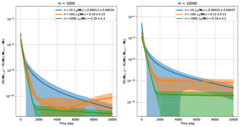
Figure 1: The gradient operator of an overparameterised shallow neural network is almost-monotone: Here, inputs are uniformly distributed on a $10$-sphere and labels are generated by $\mathbf{x}\mapsto\frac{e^{\left\langle\mathbf{W}^{\star},\mathbf{x}\right\rangle}}{1+e^{\left\langle\mathbf{W}^{\star},\mathbf{x}\right\rangle}}$ where $\mathbf{W}^{\star}$ is once sampled from $\mathcal{N}(\mathbf{0},\mathbf{I}_{10})$ at the beginning of the training. The initialisation $\mathbf{W}_{0}$ is sampled from $\mathcal{N}(\mathbf{0},\mathbf{I}_{10})$ and each experiment is performed $10$ times (which is reflected by standard deviation). The shallow network is then trained by GD with $\eta=1$, $T=10^{4}$, and sigmoid activation.

4 Additional Related Literature

Stability of Gradient Descent. Algorithmic stability (Bousquet and Elisseeff, 2002) has been used to investigate the generalisation performance of GD in a number of works (Hardt et al., 2016; Kuzborskij and Lampert, 2018; Chen et al., 2018; Lei and Ying, 2020; Richards and Rabbat, 2021). While near optimal bounds are achieved for convex losses, the non-convex case aligning with this work is more challenging. Within (Hardt et al., 2016; Kuzborskij and Lampert, 2018) in particular a restrictive $1/t$ step size is required if $t$ iterations of gradient descent are performed. This was partially alleviated within (Richards and Rabbat, 2021) which demonstrated that the magnitude of Hessian’s negative eigenvalues can be leveraged to allow for much larger step sizes to be taken. In this work we also utilise the magnitude of Hessian’s negative Eigenvalue, although a more delicate analysis is required as both: the gradient is potentially unbounded in our case; and the Hessian’s negative eigenvalues need to be bounded when evaluated across multiple points. We note the scaling of the Hessian network has also previously been observed within (Liu et al., 2020a, b), with empirical investigations into the magnitude of the Hessian’s negative Eigenvalues conducted within (Sagun et al., 2016; Yuan et al., 2019). Stability-based generalisation bounds were also shown for certain types of non-convex functions, such Polyak-Łojasiewicz functions (Charles and Papailiopoulos, 2018; Lei and Ying, 2021) and functions with strict saddles among stationary points (Gonen and Shalev-Shwartz, 2017). In line with our results, Rangamani et al. (2020) shows that for interpolating kernel predictors, minimizing the norm of the ERM solution minimizes stability.

Several works have also recently demonstrated consistency of GD with early stopping for training shallow neural networks in the presence of label noise. The concurrent work (Ji et al., 2021) also showed that shallow neural networks trained with gradient descent are consistent, although their approach distinctly different to ours e.g. leveraging structure of logistic loss as well as connections between shallow neural networks and random feature models / NTK. Earlier, Li et al. (2020) showed consistency under a certain gaussian-mixture type parametric classification model. In a more general nonparametric setting, Kuzborskij and Szepesvári (2021) showed that early-stopped GD is consistent when learning Lipschitz regression functions.

Certain notions of stability, such the uniform stability (taking $\sup$ over the data rather than expectation) allows to prove high-probability risk bounds (h.p.) (Bousquet and Elisseeff, 2002) which are known to be optimal up to log-terms (Feldman and Vondrak, 2019; Bousquet et al., 2020). In this work we show bounds in expectation, or equivalently, control the first moment of a generalisation gap. To prove a h.p. bounds while enjoying benefits of a stability in expectation, one would need to control higher order moments (Maurer, 2017; Abou-Moustafa and Szepesvári, 2019), however often this is done through a higher-order uniform stability: Since our proof closely relies on the stability in expectation, it is not clear whether our results can be trivially stated with high probability.

Notation

In the following denote $\ell(\mathbf{w},(\mathbf{x},y))\stackrel{{\scriptstyle\mathrm{def}}}{{=}}\tfrac{1}{2}(f_{\mathbf{W}}(\mathbf{x})-y)^{2}$. Unless stated otherwise, we work with vectorised quantities so $\mathbf{W}\in\mathbb{R}^{dm}$ and therefore simply interchange $\|\cdot\|_{2}$ with $\|\cdot\|_{F}$. We also use notation $(\mathbf{W})_{k}$ so select $k$-th block of size $d$, that is $(\mathbf{W})_{k}=[W_{(d-1)k+1},\ldots,W_{dk}]^{\top}$. We use notation $(a\vee b)\stackrel{{\scriptstyle\mathrm{def}}}{{=}}\max\left\{a,b\right\}$ and $(a\wedge b)\stackrel{{\scriptstyle\mathrm{def}}}{{=}}\min\left\{a,b\right\}$ throughout the paper. Let $(\mathbf{W}_{t}^{(i)})_{t}$ be the iterates of GD obtained from the data set with a resampled data point:

$$S^{(i)}\stackrel{{\scriptstyle\mathrm{def}}}{{=}}(z_{1},\ldots,z_{i-1},\widetilde{z}_{i},z_{i+1},\ldots,z_{n})$$

where $\widetilde{z}_{i}$ is an independent copy of $z_{i}$. Moreover, denote a remove-one version of $S$ by

$$S^{\backslash i}\stackrel{{\scriptstyle\mathrm{def}}}{{=}}(z_{1},\ldots,z_{i-1},z_{i+1},\ldots,z_{n})~{}.$$

Appendix A Smoothness and Curvature of the Empirical Risk (Proof of Lemma 1)

Nameddef 1 (Lemma 1 (restated)).

Fix $\mathbf{W},\widetilde{\mathbf{W}}\in\mathbb{R}^{d\times m}$. Consider 1, 2, and assume that $\mathcal{L}_{S}(\widetilde{\mathbf{W}})\leq C_{0}^{2}$. Then, for any $S$,

$$\lambda_{\max}(\nabla^{2}\mathcal{L}_{S}(\mathbf{W}))\leq\rho\quad\text{where}\quad\rho\stackrel{{\scriptstyle\mathrm{def}}}{{=}}C_{x}^{2}\left(B_{\phi^{\prime}}^{2}+B_{\phi^{\prime\prime}}B_{\phi}+\frac{B_{\phi^{\prime\prime}}C_{y}}{\sqrt{m}}\right)~{},$$

$$\min_{\alpha\in[0,1]} \lambda_{\min}(\nabla^{2}\mathcal{L}_{S}(\widetilde{\mathbf{W}}+\alpha(\mathbf{W}-\widetilde{\mathbf{W}})))\geq-\frac{B_{\phi^{\prime\prime}}\big{(}B_{\phi^{\prime}}C_{x}+C_{0}\big{)}}{\sqrt{m}}\cdot(1\vee\|\mathbf{W}-\widetilde{\mathbf{W}}\|_{F})~{}.$$ (10)

Proof.

Vectorising allows the loss’s Hessian to be denoted

$$\nabla^{2}\ell(\mathbf{W},z)=\nabla f_{\mathbf{W}}(\mathbf{x})\nabla f_{\mathbf{W}}(\mathbf{x})^{\top}+\nabla^{2}f_{\mathbf{W}}(\mathbf{x})(f_{\mathbf{W}}(\mathbf{x})-y)$$ (11)

where

$$\nabla f_{\mathbf{W}}(\mathbf{x})=\begin{pmatrix}u_{1}\mathbf{x}\phi^{\prime}\left(\langle(\mathbf{W})_{1},\mathbf{x}\rangle\right)\\ u_{2}\mathbf{x}\phi^{\prime}\left(\langle(\mathbf{W})_{2},\mathbf{x}\rangle\right)\\ \vdots\\ u_{m}\mathbf{x}\phi^{\prime}\left(\langle(\mathbf{W})_{m},\mathbf{x}\rangle\right)\end{pmatrix}\in\mathbb{R}^{dm}$$

and $\nabla^{2}f_{\mathbf{W}}(\mathbf{x})\in\mathbb{R}^{dm\times dm}$ with

$$\nabla^{2}f_{\mathbf{W}}(\mathbf{x})=\begin{pmatrix}u_{1}\mathbf{x}\mathbf{x}^{\top}\phi^{\prime\prime}(\langle(\mathbf{W})_{1},\mathbf{x}\rangle)&0&0&\dots&0\\ 0&u_{2}\mathbf{x}\mathbf{x}^{\top}\phi^{\prime\prime}(\langle(\mathbf{W})_{2},\mathbf{x}\rangle)&0&\dots&0\\ \vdots&\ddots&\ddots&\vdots&\vdots\\ 0&0&0&\dots&u_{m}\mathbf{x}\mathbf{x}^{\top}\phi^{\prime\prime}(\langle(\mathbf{W})_{m},\mathbf{x}\rangle)\end{pmatrix}$$

Note that we then immediately have with $\mathbf{v}=(\mathbf{v}_{1},\mathbf{v}_{2},\dots,\mathbf{v}_{m})\in\mathbb{R}^{dm}$ with $\mathbf{v}_{i}\in\mathbb{R}^{d}$

$$\|\nabla^{2}f_{\mathbf{W}}(\mathbf{x})\|_{2} =\max_{\mathbf{v}:\|\mathbf{v}\|_{2}\leq 1}\sum_{j=1}^{m}u_{j}\langle\mathbf{v}_{j},\mathbf{x}\rangle^{2}\phi^{\prime\prime}(\langle(\mathbf{W})_{j},\mathbf{x}\rangle)$$

$$\leq\frac{1}{\sqrt{m}}\|\mathbf{x}\|_{2}^{2}B_{\phi^{\prime\prime}}\max_{\mathbf{v}:\|\mathbf{v}\|_{2}\leq 1}\sum_{j=1}^{m}\|\mathbf{v}_{j}\|_{2}^{2}$$

$$\leq\frac{C^{2}_{x}B_{\phi^{\prime\prime}}}{\sqrt{m}}~{}.$$ (12)

We then see that the maximum Eigenvalue of the Hessian is upper bounded for any $\mathbf{W}\in\mathbb{R}^{dm}$, that is

$$\|\nabla^{2}\ell(\mathbf{W},z)\|_{2} \leq\|\nabla f_{\mathbf{W}}(\mathbf{x})\|_{2}^{2}+\|\nabla^{2}f_{\mathbf{W}}(\mathbf{x})\|_{2}|f_{\mathbf{W}}(\mathbf{x})-y|$$ (13)

$$\leq C_{x}^{2}B_{\phi^{\prime}}^{2}+\frac{C_{x}^{2}B_{\phi^{\prime\prime}}}{\sqrt{m}}(\sqrt{m}B_{\phi}+C_{y})$$ (14)

and therefore the objective is $\rho$-smooth with $\rho=C_{x}^{2}\big{(}B_{\phi^{\prime}}^{2}+B_{\phi^{\prime\prime}}B_{\phi}+\frac{B_{\phi^{\prime\prime}}C_{y}}{\sqrt{m}}\big{)}$.

Let us now prove the lower bound (10). For some fixed $\mathbf{W},\widetilde{\mathbf{W}}\in\mathbb{R}^{d\times m}$ define

$$\mathbf{W}(\alpha)\stackrel{{\scriptstyle\mathrm{def}}}{{=}}\widetilde{\mathbf{W}}+\alpha(\mathbf{W}-\widetilde{\mathbf{W}})\qquad\alpha\in[0,1]~{}.$$

Looking at the Hessian in (11), the first matrix is positive semi-definite, therefore

$$\lambda_{\min}(\nabla^{2}\mathcal{L}_{S}(\mathbf{W}(\alpha))) \geq-\Big{(}\max_{i=1,\dots,n}\big{\{}\|\nabla^{2}f_{\mathbf{W}(\alpha)}(\mathbf{x}_{i})\|_{2}\big{\}}\Big{)}\frac{1}{n}\sum_{i=1}^{n}|f_{\mathbf{W}(\alpha)}(\mathbf{x}_{i})-y_{i}|$$

$$\geq-\frac{C_{x}^{2}B_{\phi^{\prime\prime}}}{\sqrt{m}}\cdot\frac{1}{n}\sum_{i=1}^{n}|f_{\mathbf{W}(\alpha)}(\mathbf{x}_{i})-y_{i}|$$

where we have used the upper bound on $\|\nabla^{2}f_{\mathbf{W}}(\mathbf{x}_{i})\|_{2}$. Adding and subtracting $f_{\widetilde{\mathbf{W}}}(\mathbf{x}_{i})$ inside the absolute value we then get

$$\frac{1}{n}\sum_{i=1}^{n}|f_{\mathbf{W}(\alpha)}(\mathbf{x}_{i})-y_{i}| \leq\frac{1}{n}\sum_{i=1}^{n}|f_{\mathbf{W}(\alpha)}(\mathbf{x}_{i})-f_{\widetilde{\mathbf{W}}}(\mathbf{x}_{i})|+\frac{1}{n}\sum_{i=1}^{n}|f_{\widetilde{\mathbf{W}}}(\mathbf{x}_{i})-y_{i}|$$

$$\leq B_{\phi^{\prime}}C_{x}\|\mathbf{W}(\alpha)-\widetilde{\mathbf{W}}\|_{2}+\sqrt{\mathcal{L}_{S}(\widetilde{\mathbf{W}})}$$

$$\leq B_{\phi^{\prime}}C_{x}\|\mathbf{W}(\alpha)-\widetilde{\mathbf{W}}\|_{2}+\sqrt{\mathcal{L}_{S}(\mathbf{W}_{0})}$$

$$\leq\big{(}B_{\phi^{\prime}}C_{x}+C_{0}\big{)}(1\vee\|\mathbf{W}(\alpha)-\widetilde{\mathbf{W}}\|_{2})$$

where for the second term we have simply applied Cauchy-Schwarz inequality. For the first term, we used that for any $\mathbf{W},\widetilde{\mathbf{W}}\in\mathbb{R}^{dm}$ we see that

$$|f_{\mathbf{W}}(\mathbf{x})-f_{\widetilde{\mathbf{W}}}(\mathbf{x})| \leq\frac{1}{\sqrt{m}}\sum_{i=1}^{m}|\phi(\langle(\mathbf{W})_{i},\mathbf{x}\rangle)-\phi(\langle(\widetilde{\mathbf{W}})_{i},\mathbf{x}\rangle)|$$ (15)

$$\leq\frac{B_{\phi^{\prime}}}{\sqrt{m}}\sum_{i=1}^{m}\left|\langle(\mathbf{W})_{i}-(\widetilde{\mathbf{W}})_{i},\mathbf{x}\rangle\right|$$

$$\leq C_{x}B_{\phi^{\prime}}\|\mathbf{W}-\widetilde{\mathbf{W}}\|_{2}.$$ (16)

Bringing everything together yields the desired lower bound

$$\lambda_{\min}(\nabla^{2}\mathcal{L}_{S}(\mathbf{W}(\alpha))) \geq-\frac{C_{x}^{2}}{\sqrt{m}}B_{\phi^{\prime\prime}}\big{(}B_{\phi^{\prime}}C_{x}+C_{0}\big{)}(1\vee\|\mathbf{W}(\alpha)-\widetilde{\mathbf{W}}\|_{2})$$

$$\geq-\frac{C_{x}^{2}}{\sqrt{m}}B_{\phi^{\prime\prime}}\big{(}B_{\phi^{\prime}}C_{x}+C_{0}\big{)}(1\vee\|\mathbf{W}-\widetilde{\mathbf{W}}\|_{2})~{}.$$

This holds for any $\alpha\in[0,1]$, therefore, we took the minimum. ∎

Appendix B Optimisation Error Bound (Proof of Lemma 2)

In this section we present the proof for the Optimisation Error term. We begin by quoting the result which we set to prove.

Nameddef 2 (Lemma 2 (restated)).

Consider Assumptions 1 and 2. Fix $t>0$. If $\eta\leq 1/(2\rho)$, then

$$\frac{1}{t}\sum_{j=0}^{t}\mathcal{L}_{S}(\mathbf{W}_{j})\leq\min_{\mathbf{W}\in\mathbb{R}^{d\times m}}\Big{\{}\mathcal{L}_{S}(\mathbf{W})+\frac{\|\mathbf{W}-\mathbf{W}_{0}\|_{F}^{2}}{\eta t}+\frac{\widetilde{b}\|\mathbf{W}-\mathbf{W}_{0}\|_{F}^{3}}{\sqrt{m}}\Big{\}}+\widetilde{b}C_{0}\cdot\frac{(\eta t)^{\frac{3}{2}}}{\sqrt{m}}$$

where $\widetilde{b}=C_{x}^{2}B_{\phi^{\prime\prime}}\left(B_{\phi^{\prime}}C_{x}+C_{0}\right)$.

Proof.

Using Lemma 1 as well as that $\eta\rho\leq 1$ from the assumption within the theorem yields for $t\geq 0$

$$\mathcal{L}_{S}(\mathbf{W}_{t+1}) \leq\mathcal{L}_{S}(\mathbf{W}_{t})-\eta\big{(}1-\frac{\eta\rho}{2}\big{)}\|\nabla\mathcal{L}_{S}(\mathbf{W}_{t})\|_{2}^{2}$$

$$\leq\mathcal{L}_{S}(\mathbf{W}_{t})-\frac{\eta}{2}\|\nabla\mathcal{L}_{S}(\mathbf{W}_{t})\|_{2}^{2}.$$

Fix some $\mathbf{W}\in\mathbb{R}^{dm}$. We then use the following inequality which will be proven shortly:

$$\mathcal{L}_{S}(\mathbf{W}_{t})\leq\mathcal{L}_{S}(\mathbf{W})-\langle\mathbf{W}-\mathbf{W}_{t},\nabla\mathcal{L}_{S}(\mathbf{W}_{t})\rangle+\frac{\widetilde{b}}{\sqrt{m}}\big{(}1\vee\|\mathbf{W}-\mathbf{W}_{t}\|_{2}\big{)}^{3}$$ (17)

Plugging in this inequality we then get

$$\mathcal{L}_{S}(\mathbf{W}_{t+1})\leq\mathcal{L}_{S}(\mathbf{W})-\langle\mathbf{W}-\mathbf{W}_{t},\nabla\mathcal{L}_{S}(\mathbf{W}_{t})\rangle-\frac{\eta}{2}\|\nabla\mathcal{L}_{S}(\mathbf{W}_{t})\|_{2}^{2}+\frac{\widetilde{b}}{\sqrt{m}}\big{(}1\vee\|\mathbf{W}-\mathbf{W}_{t}\|_{2}\big{)}^{3}~{}.$$

Note that we can rewrite

$$-\langle\mathbf{W}-\mathbf{W}_{t},\nabla\mathcal{L}_{S}(\mathbf{W}_{t})\rangle-\frac{\eta}{2}\|\nabla\mathcal{L}_{S}(\mathbf{W}_{t})\|_{2}^{2}$$

$$=\frac{1}{\eta}\langle\mathbf{W}-\mathbf{W}_{t},\mathbf{W}_{t+1}-\mathbf{W}_{t}\rangle-\frac{1}{2\eta}\|\mathbf{W}_{t+1}-\mathbf{W}_{t}\|_{2}^{2}$$

$$=\frac{1}{\eta}\big{(}\|\mathbf{W}-\mathbf{W}_{t}\|_{2}^{2}-\|\mathbf{W}_{t+1}-\mathbf{W}\|_{2}^{2}\big{)}$$

where we used that for any vectors $\mathbf{x},\mathbf{y},\mathbf{z}$: $2\langle\mathbf{x}-\mathbf{y},\mathbf{x}-\mathbf{z}\rangle=\|\mathbf{x}-\mathbf{y}\|_{2}^{2}+\|\mathbf{x}-\mathbf{z}\|_{2}^{2}-\|\mathbf{y}-\mathbf{z}\|_{2}^{2}$ (which is easier to see if we relabel $2\langle\mathbf{a},\mathbf{b}\rangle=\|\mathbf{a}\|_{2}^{2}+\|\mathbf{b}\|_{2}^{2}-\|\mathbf{a}-\mathbf{b}\|_{2}^{2}$). Plugging in and summing up we get

$$\frac{1}{t}\sum_{s=0}^{t}\mathcal{L}_{S}(\mathbf{W}_{t})\leq\mathcal{L}_{S}(\mathbf{W})+\frac{\|\mathbf{W}-\mathbf{W}_{0}\|_{2}^{2}}{\eta t}+\frac{\widetilde{b}}{\sqrt{m}}\cdot\frac{1}{t}\sum_{s=0}^{t}\big{(}1\vee\|\mathbf{W}-\mathbf{W}_{t}\|_{2}\big{)}^{3}.$$

Since the choice of $\mathbf{W}$ was arbitrary, we can simply take the minimum.

Proof of Eq. 17.

Let us now prove the key Eq. 17. Fix $t\geq 0$, and let us define the following functions for $\alpha\in[0,1]$

$$\mathbf{W}(\alpha) \stackrel{{\scriptstyle\mathrm{def}}}{{=}}\mathbf{W}_{t}+\alpha(\mathbf{W}-\mathbf{W}_{t})~{},$$

$$g(\alpha) \stackrel{{\scriptstyle\mathrm{def}}}{{=}}\mathcal{L}_{S}(\mathbf{W}(\alpha))+\frac{\widetilde{b}}{\sqrt{m}}\cdot\frac{\alpha^{2}}{2}\big{(}1\vee\|\mathbf{W}-\mathbf{W}_{t}\|_{2}\big{)}^{3}~{}.$$

Note that computing the derivative we have

$$g^{\prime\prime}(\alpha)=(\mathbf{W}-\mathbf{W}_{t})^{\top}\nabla^{2}\mathcal{L}_{S}(\mathbf{W}(\alpha))(\mathbf{W}-\mathbf{W}_{t})+\frac{\widetilde{b}}{\sqrt{m}}\big{(}1\vee\|\mathbf{W}-\mathbf{W}_{t}\|_{2}\big{)}^{3}.$$

On the other hand by Lemma 1 we have

$$\min_{\alpha\in[0,1]}\lambda_{\min}(\nabla^{2}\mathcal{L}_{S}(\mathbf{W}(\alpha)))\geq-\frac{\widetilde{b}}{\sqrt{m}}\big{(}1\vee\|\mathbf{W}-\mathbf{W}_{t}\|_{2}\big{)}$$

and we immediately have $g^{\prime\prime}(\alpha)\geq 0$, and thus, $g(\cdot)$ is convex on $[0,1]$. Inequality (17) then arises from $g(1)-g(0)\geq g^{\prime}(0)$, in particular

$$g(1)-g(0) =\mathcal{L}_{S}(\mathbf{W})+\frac{\widetilde{b}}{\sqrt{m}}\big{(}1\vee\|\mathbf{W}-\mathbf{W}_{t}\|_{2}\big{)}^{3}-\mathcal{L}_{S}(\mathbf{W}_{t})$$

$$\geq\langle\mathbf{W}-\mathbf{W}_{t},\nabla\mathcal{L}_{S}(\mathbf{W}_{t})\rangle$$

$$=g^{\prime}(0)$$

as required. ∎

Appendix C Generalisation Gap Bound (Proof of Theorem 1)

In this section we prove:

Nameddef 3 (Theorem 1 (restated)).

Consider Assumptions 1 and 2. Fix $t>0$. If $\eta\leq 1/(2\rho)$ and

$$m\geq 144(\eta t)^{2}C_{x}^{4}C_{0}^{2}B_{\phi^{\prime\prime}}^{2}\left(4B_{\phi^{\prime}}C_{x}\sqrt{\eta t}+\sqrt{2}\right)^{2}$$

$$\mathrm{then}\qquad \mathbf{E}\left[\epsilon^{\text{Gen}}(\mathbf{W}_{t+1})\;\middle|\;\mathbf{W}_{0},\mathbf{u}\right]\leq b\left(\frac{\eta}{n}+\frac{\eta^{2}t}{n^{2}}\right)\sum_{j=0}^{t}\mathbf{E}\left[\mathcal{L}_{S}(\mathbf{W}_{j})\;\middle|\;\mathbf{W}_{0},\mathbf{u}\right]$$

where $b=16e^{3}C_{x}^{\frac{3}{2}}B_{\phi^{\prime}}^{2}(1+C_{x}^{\frac{3}{2}}B_{\phi^{\prime}}^{2})$.

To prove this result we use algorithmic stability arguments. Recall that we can write [Shalev-Shwartz and Ben-David, 2014, Chapter 13],

$$\mathbf{E}\left[\mathcal{L}(\mathbf{W}_{t+1})-\mathcal{L}_{S}(\mathbf{W}_{t+1})\;\middle|\;\mathbf{W}_{0},\mathbf{u}\right]=\frac{1}{n}\sum_{i=1}^{n}\mathbf{E}\left[\ell(\mathbf{W}_{t+1},\widetilde{z}_{i})-\ell(\mathbf{W}_{t+1}^{(i)},\widetilde{z}_{i})\;\middle|\;\mathbf{W}_{0},\mathbf{u}\right]~{}.$$

The following lemma shown in Section C.1 then bounds the Generalisation error in terms of a notation of stability.

Nameddef 4 (Lemma 3 (restated)).

Consider Assumptions 1 and 2. Then, for any $t\geq 0$,

$$\mathbf{E}\left[\mathcal{L}(\mathbf{W}_{t})-\mathcal{L}_{S}(\mathbf{W}_{t})\;\middle|\;\mathbf{W}_{0},\mathbf{u}\right]$$

$$\leq B_{\phi^{\prime}}\sqrt{C_{x}}\sqrt{\mathbf{E}\left[\mathcal{L}_{S}(\mathbf{W}_{t})\;\middle|\;\mathbf{W}_{0},\mathbf{u}\right]}\sqrt{\frac{1}{n}\sum_{i=1}^{n}\mathbf{E}\left[\|\mathbf{W}_{t}-\mathbf{W}_{t}^{(i)}\|_{\text{op}}^{2}\;\middle|\;\mathbf{W}_{0},\mathbf{u}\right]}$$

$$+C_{x}B_{\phi^{\prime}}^{2}\cdot\frac{1}{n}\sum_{i=1}^{n}\mathbf{E}\left[\|\mathbf{W}_{t}-\mathbf{W}_{t}^{(i)}\|_{\text{op}}^{2}\;\middle|\;\mathbf{W}_{0},\mathbf{u}\right]$$

where $\|\cdot\|_{\text{op}}$ denotes the spectral norm.

We note while the stability is only required on the spectral norm, our bound will be on the element wise $L_{2}$-norm i.e. Frobenius norm, which upper bounds the spectral norm. It is summarised within the following lemma shown in Section C.2.

Lemma 4 (Bound on On-Average Parameter Stability).

Consider Assumptions 1 and 2. Fix $t>0$. If $\eta\leq 1/(2\rho)$, then

$$\frac{1}{n}\sum_{i=1}^{n}\mathbf{E}\left[\|\mathbf{W}_{t+1}-\mathbf{W}_{t+1}^{(i)}\|_{F}^{2}\;\middle|\;\mathbf{W}_{0},\mathbf{u}\right]\leq 8e\frac{\eta^{2}t}{n^{2}}\Big{(}\frac{1}{1-2\eta\epsilon}\Big{)}^{t}\frac{1}{n}\sum_{i=1}^{n}\sum_{j=0}^{t}\mathbf{E}\left[\|\nabla\ell(\mathbf{W}_{j},z_{i})\|_{2}^{2}\;\middle|\;\mathbf{W}_{0},\mathbf{u}\right]$$

where $\epsilon=2\cdot\frac{C_{x}^{2}\sqrt{C_{0}}B_{\phi^{\prime\prime}}}{\sqrt{m}}\big{(}4B_{\phi^{\prime}}C_{x}\sqrt{\eta t}+\sqrt{2}\big{)}$.

Theorem 1 then arises by combining Lemma 3 and Lemma 4, and noting the following three points. Firstly, recall that

$$\frac{1}{n}\sum_{i=1}^{n}\|\nabla\ell(\mathbf{W},z_{i})\|_{2}^{2} \leq\big{(}\max_{i=1,\dots,n}\|\nabla f_{\mathbf{W}}(\mathbf{x}_{i})\|_{2}^{2}\big{)}\frac{1}{n}\sum_{i=1}^{n}(f_{\mathbf{W}}(\mathbf{x}_{i})-y_{i})^{2}$$

$$\leq 2C_{x}^{2}B_{\phi^{\prime}}^{2}\mathcal{L}_{S}(\mathbf{W}).$$

Secondly, note that we have $\big{(}\frac{1}{1-2\eta\epsilon}\big{)}^{t}\leq\exp(\frac{2\eta t\epsilon}{1-2\eta t\epsilon})\leq e^{2}$ when $2\eta t\epsilon\leq 2/3$. For this to occur we then require

$$\epsilon=2\cdot\frac{C_{x}^{2}\sqrt{C_{0}}B_{\phi^{\prime\prime}}}{\sqrt{m}}\cdot\big{(}4B_{\phi^{\prime}}C_{x}\sqrt{\eta t}+\sqrt{2}\big{)}\leq\frac{1}{3\eta t},$$

which is satisfied by scaling $m$ sufficient large, in particular, as required within condition (7) within the statement of Theorem 1. This allows us to arrive at the bound on the $L_{2}$-stability

$$\frac{1}{n}\sum_{i=1}^{n}\mathbf{E}\left[\|\mathbf{W}_{t+1}-\mathbf{W}_{t+1}^{(i)}\|_{F}^{2}\;\middle|\;\mathbf{W}_{0},\mathbf{u}\right]\leq\frac{\eta^{2}t}{n^{2}}\cdot 16e^{3}C_{x}^{2}B_{\phi^{\prime}}^{2}\sum_{j=0}^{t}\mathbf{E}\left[\mathcal{L}_{S}(\mathbf{W}_{j})\;\middle|\;\mathbf{W}_{0},\mathbf{u}\right]~{}.$$

Third and finally, note that we can bound

$$\sqrt{\mathbf{E}\left[\mathcal{L}_{S}(\mathbf{W}_{t+1})\;\middle|\;\mathbf{W}_{0},\mathbf{u}\right]}\sqrt{\frac{\eta^{2}t}{n^{2}}\sum_{j=0}^{t}\mathbf{E}\left[\mathcal{L}_{S}(\mathbf{W}_{j})\;\middle|\;\mathbf{W}_{0},\mathbf{u}\right]}$$

$$=\frac{\eta}{n}\sqrt{t\mathbf{E}\left[\mathcal{L}_{S}(\mathbf{W}_{t+1})\;\middle|\;\mathbf{W}_{0},\mathbf{u}\right]}\sqrt{\sum_{j=0}^{t}\mathbf{E}\left[\mathcal{L}_{S}(\mathbf{W}_{j})\;\middle|\;\mathbf{W}_{0},\mathbf{u}\right]}$$

$$\leq\frac{\eta}{n}\sum_{j=0}^{t}\mathbf{E}\left[\mathcal{L}_{S}(\mathbf{W}_{j})\;\middle|\;\mathbf{W}_{0},\mathbf{u}\right]$$

since $\mathcal{L}_{S}(\mathbf{W}_{t+1})\leq\frac{1}{t}\sum_{j=1}^{t}\mathcal{L}_{S}(\mathbf{W}_{j})$. This then results in

$$\mathbf{E}\left[\mathcal{L}(\mathbf{W}_{t+1})-\mathcal{L}_{S}(\mathbf{W}_{t+1})\;\middle|\;\mathbf{W}_{0},\mathbf{u}\right]$$

$$\leq\Big{(}\frac{\eta}{n}\big{(}4e^{2}C_{x}^{3/2}B_{\phi^{\prime}}^{2}\big{)}+\frac{\eta^{2}t}{n^{2}}\big{(}16e^{3}C_{x}^{3}B_{\phi^{\prime}}^{4}\big{)}\Big{)}\sum_{j=0}^{t}\mathbf{E}\left[\mathcal{L}_{S}(\mathbf{W}_{j})\;\middle|\;\mathbf{W}_{0},\mathbf{u}\right]$$

$$\leq 16e^{3}C_{x}^{3/2}B_{\phi^{\prime}}^{2}(1+C_{x}^{3/2}B_{\phi^{\prime}}^{2})\Big{(}\frac{\eta}{n}+\frac{\eta^{2}t}{n^{2}}\Big{)}\sum_{j=0}^{t}\mathbf{E}\left[\mathcal{L}_{S}(\mathbf{W}_{j})\;\middle|\;\mathbf{W}_{0},\mathbf{u}\right]$$

as required.

C.1 Proof of Lemma 3: From loss stability to parameter stability

Recall that $\widetilde{z}_{i}=(\widetilde{\mathbf{x}}_{i},y_{i})\in\mathcal{B}_{2}^{d}(C_{x})\times[-C_{y},C_{y}]$. Expanding the square loss and some basic algebra gives us:

$$2\left(\ell(\mathbf{W}_{t},\widetilde{z}_{i})-\ell(\mathbf{W}_{t}^{(i)},\widetilde{z}_{i})\right)$$

$$=\left(f_{\mathbf{W}_{t}}(\widetilde{\mathbf{x}}_{i})-\widetilde{y}_{i}\right)^{2}-\left(f_{\mathbf{W}_{t}^{(i)}}(\widetilde{\mathbf{x}}_{i})-\widetilde{y}_{i}\right)^{2}$$

$$=\left(f_{\mathbf{W}_{t}}(\widetilde{\mathbf{x}}_{i})-\widetilde{y}_{i}\right)\left(f_{\mathbf{W}_{t}}(\widetilde{\mathbf{x}}_{i})-f_{\mathbf{W}_{t}^{(i)}}(\widetilde{\mathbf{x}}_{i})\right)+\left(f_{\mathbf{W}_{t}^{(i)}}(\widetilde{\mathbf{x}}_{i})-\widetilde{y}_{i}\right)\left(f_{\mathbf{W}_{t}}(\widetilde{\mathbf{x}}_{i})-f_{\mathbf{W}_{t}^{(i)}}(\widetilde{\mathbf{x}}_{i})\right)$$

$$=\left(f_{\mathbf{W}_{t}}(\widetilde{\mathbf{x}}_{i})-f_{\mathbf{W}_{t}^{(i)}}(\widetilde{\mathbf{x}}_{i})\right)^{2}+2\left(f_{\mathbf{W}_{t}^{(i)}}(\widetilde{\mathbf{x}}_{i})-\widetilde{y}_{i}\right)\left(f_{\mathbf{W}_{t}}(\widetilde{\mathbf{x}}_{i})-f_{\mathbf{W}_{t}^{(i)}}(\widetilde{\mathbf{x}}_{i})\right)~{}.$$

We then have

$$\frac{1}{n}\sum_{i=1}^{n}\mathbf{E}\left[\ell(\mathbf{W}_{t},\widetilde{z}_{i})-\ell(\mathbf{W}_{t}^{(i)},\widetilde{z}_{i})\;\middle|\;\mathbf{W}_{0},\mathbf{u}\right]$$

$$\leq\frac{1}{n}\sum_{i=1}^{n}\mathbf{E}\left[\left|\left(f_{\mathbf{W}_{t}^{(i)}}(\widetilde{\mathbf{x}}_{i})-\widetilde{y}_{i}\right)\right|\left|\left(f_{\mathbf{W}_{t}}(\widetilde{\mathbf{x}}_{i})-f_{\mathbf{W}_{t}^{(i)}}(\widetilde{\mathbf{x}}_{i})\right)\right|\;\middle|\;\mathbf{W}_{0},\mathbf{u}\right]$$

$$\quad\quad+\frac{1}{2n}\sum_{i=1}^{n}\mathbf{E}\left[\left(f_{\mathbf{W}_{t}}(\widetilde{\mathbf{x}}_{i})-f_{\mathbf{W}_{t}^{(i)}}(\widetilde{\mathbf{x}}_{i})\right)^{2}\;\middle|\;\mathbf{W}_{0},\mathbf{u}\right]$$

$$\leq\sqrt{\frac{1}{n}\sum_{i=1}^{n}\mathbf{E}\left[\left(f_{\mathbf{W}_{t}^{(i)}}(\widetilde{\mathbf{x}}_{i})-\widetilde{y}_{i}\right)^{2}\;\middle|\;\mathbf{W}_{0},\mathbf{u}\right]}\sqrt{\frac{1}{n}\sum_{i=1}^{n}\mathbf{E}\left[\left(f_{\mathbf{W}_{t}}(\widetilde{\mathbf{x}}_{i})-f_{\mathbf{W}_{t}^{(i)}}(\widetilde{\mathbf{x}}_{i})\right)^{2}\;\middle|\;\mathbf{W}_{0},\mathbf{u}\right]}$$

$$\quad\quad+\frac{1}{2n}\sum_{i=1}^{n}\mathbf{E}\left[\left(f_{\mathbf{W}_{t}}(\widetilde{\mathbf{x}}_{i})-f_{\mathbf{W}_{t}^{(i)}}(\widetilde{\mathbf{x}}_{i})\right)^{2}\;\middle|\;\mathbf{W}_{0},\mathbf{u}\right]$$

where performing steps as in Eq. 15-(16) we have

$$\left(f_{\mathbf{W}_{t}}(\widetilde{\mathbf{x}}_{i})-f_{\mathbf{W}_{t}^{(i)}}(\widetilde{\mathbf{x}}_{i})\right)^{2}\leq C^{2}_{x}B_{\phi^{\prime}}^{2}\|\mathbf{W}_{t}-\mathbf{W}_{t}^{(i)}\|_{2}^{2}~{}.$$

Plugging in this bound then yields the result.

C.2 Proof of Lemma 4: Bound on on-average parameter stability

Throughout the proof empirical risk w.r.t. remove-one tuple $S^{\backslash i}$ is denoted as

$$\mathcal{L}_{S^{\backslash i}}(\mathbf{W})=\mathcal{L}_{S}(\mathbf{W})-\frac{1}{n}\ell(\mathbf{W},z_{i})=\mathcal{L}_{S_{i}}(\mathbf{W})-\frac{1}{n}\ell(\mathbf{W},\widetilde{z}_{i})~{}.$$

Plugging in the gradient updates with the inequality $(a+b)^{2}\leq(1+p)a^{2}+(1+1/p)b^{2}$ for $p>0$ then yields (this technique having been applied within [Lei and Ying, 2020])

$$\|\mathbf{W}_{t+1}-\mathbf{W}_{t+1}^{(i)}\|_{2}^{2} \leq(1+p)\underbrace{\|\mathbf{W}_{t}-\mathbf{W}_{t}^{(i)}-\eta\left(\nabla\mathcal{L}_{S^{\backslash i}}(\mathbf{W}_{t})-\nabla\mathcal{L}_{S^{\backslash i}}(\mathbf{W}_{t}^{(i)})\right)\|_{2}^{2}}_{\text{Expansiveness of the Gradient Update}}$$

$$+(1+1/p)\cdot\frac{2\eta^{2}}{n^{2}}\cdot\left(\|\nabla\ell(\mathbf{W}_{t},z_{i})\|_{2}^{2}+\|\nabla\ell(\mathbf{W}_{t}^{(i)}),\widetilde{z}_{i})\|_{2}^{2}\right)~{}.$$

We must now bound the expansiveness of the gradient update. Opening-up the squared norm we get

$$\|\mathbf{W}_{t}-\mathbf{W}_{t}^{(i)}-\eta(\nabla\mathcal{L}_{S^{\backslash i}}(\mathbf{W}_{t})-\nabla\mathcal{L}_{S^{\backslash i}}(\mathbf{W}_{t}^{(i)}))\|_{2}^{2}$$

$$=\|\mathbf{W}_{t}-\mathbf{W}_{t}^{(i)}\|^{2}_{2}+\eta^{2}\|\nabla\mathcal{L}_{S^{\backslash i}}(\mathbf{W}_{t})-\nabla\mathcal{L}_{S^{\backslash i}}(\mathbf{W}_{t}^{(i)})\|_{2}^{2}$$

$$\quad\quad-2\eta\left\langle\mathbf{W}_{t}-\mathbf{W}_{t}^{(i)},\nabla\mathcal{L}_{S^{\backslash i}}(\mathbf{W}_{t})-\nabla\mathcal{L}_{S^{\backslash i}}(\mathbf{W}_{t}^{(i)})\right\rangle$$

For this purpose we will use the following key lemma shown in Section C.3.1:

Lemma 5 (Almost Co-coercivity of the Gradient Operator).

Consider the assumptions of Lemma 4. Then for $t\geq 1$

$$\langle\mathbf{W}_{t}-\mathbf{W}_{t}^{(i)},\nabla\mathcal{L}_{S^{\backslash i}}(\mathbf{W}_{t})-\nabla\mathcal{L}_{S^{\backslash i}}(\mathbf{W}_{t}^{(i)})\rangle\geq 2\eta\left(1-\frac{\eta\rho}{2}\right)\|\nabla\mathcal{L}_{S^{\backslash i}}(\mathbf{W}_{t})-\nabla\mathcal{L}_{S^{\backslash i}}(\mathbf{W}_{t}^{(i)})\|_{2}^{2}$$

$$\quad\quad\quad\quad\quad\quad-\epsilon\left\|\mathbf{W}_{t}-\mathbf{W}_{t}^{(i)}-\eta\left(\nabla\mathcal{L}_{S^{\backslash i}}(\mathbf{W}_{t})-\nabla\mathcal{L}_{S^{\backslash i}}(\mathbf{W}_{t}^{(i)})\right)\right\|_{2}^{2}$$

where

$$\rho =C_{x}^{2}\left(B_{\phi^{\prime}}^{2}+B_{\phi^{\prime\prime}}B_{\phi}+\frac{B_{\phi^{\prime\prime}}C_{y}}{\sqrt{m}}\right)~{},$$

$$\epsilon =2\cdot\frac{C_{x}^{2}\sqrt{C_{0}}B_{\phi^{\prime\prime}}}{\sqrt{m}}\left(4B_{\phi^{\prime}}C_{x}\sqrt{\eta t}+\sqrt{2}\right)~{}.$$

Thus by Lemma 5 we get

$$\|\mathbf{W}_{t}-\mathbf{W}_{t}^{(i)}-\eta\left(\nabla\mathcal{L}_{S^{\backslash i}}(\mathbf{W}_{t})-\nabla\mathcal{L}_{S^{\backslash i}}(\mathbf{W}_{t}^{(i)})\right)\|_{2}^{2}$$

$$\leq\|\mathbf{W}_{t}-\mathbf{W}_{t}^{(i)}\|_{2}^{2}+\eta^{2}(2\eta\rho-3)\left\|\nabla\mathcal{L}_{S^{\backslash i}}(\mathbf{W}_{t})-\nabla\mathcal{L}_{S^{\backslash i}}(\mathbf{W}_{t}^{(i)})\right\|_{2}^{2}$$

$$\quad\quad+2\eta\epsilon\left\|\mathbf{W}_{t}-\mathbf{W}_{t}^{(i)}-\eta\left(\nabla\mathcal{L}_{S^{\backslash i}}(\mathbf{W}_{t})-\nabla\mathcal{L}_{S^{\backslash i}}(\mathbf{W}_{t}^{(i)})\right)\right\|_{2}^{2}.$$

Rearranging and using that $\eta\rho\leq 1/2$ we then arrive at the recursion

$$\|\mathbf{W}_{t+1}-\mathbf{W}_{t+1}^{(i)}\|_{F}^{2} \leq\frac{1+p}{1-2\eta\epsilon}\cdot\|\mathbf{W}_{t}-\mathbf{W}_{t}^{(i)}\|_{F}^{2}$$

$$\quad\quad+\left(1+\frac{1}{p}\right)\cdot\frac{2\eta^{2}}{n^{2}}\left(\|\nabla\ell(\mathbf{W}_{t},z_{i})\|_{2}^{2}+\|\nabla\ell(\mathbf{W}_{t}^{(i)}),\widetilde{z}_{i})\|_{2}^{2}\right)$$

$$\leq\left(1+\frac{1}{p}\right)\cdot\frac{2\eta^{2}}{n^{2}}\left(\frac{1+p}{1-2\eta\epsilon}\right)^{t}\sum_{j=0}^{t}\left(\|\nabla\ell(\mathbf{W}_{j},z_{i})\|_{2}^{2}+\|\nabla\ell(\mathbf{W}_{j}^{(i)}),\widetilde{z}_{i})\|_{2}^{2}\right)~{}.$$

Taking expectation and summing we then get

$$\frac{1}{n}\sum_{i=1}^{n}\mathbf{E}\left[\|\mathbf{W}_{t+1}-\mathbf{W}_{t+1}^{(i)}\|_{F}^{2}\;\middle|\;\mathbf{W}_{0},\mathbf{u}\right]$$

$$\qquad\qquad\leq 4(1+1/p)\frac{2\eta^{2}}{n^{2}}\left(\frac{(1+p)}{1-2\eta\epsilon}\right)^{t}\sum_{j=0}^{t}\mathbf{E}\left[\|\nabla\ell(\mathbf{W}_{j},z_{i})\|_{2}^{2}\;\middle|\;\mathbf{W}_{0},\mathbf{u}\right]$$

where we note that $\mathbf{E}\left[\|\nabla\ell(\mathbf{W}_{j},z_{i})\|_{2}^{2}\;\middle|\;\mathbf{W}_{0},\mathbf{u}\right]=\mathbf{E}\left[\|\nabla\ell(\mathbf{W}_{j}^{(i)},\widetilde{z}_{i})\|_{2}^{2}\;\middle|\;\mathbf{W}_{0},\mathbf{u}\right]$ since $z_{i}$ and $\widetilde{z}_{i}$ are identically distributed. Picking $p=1/t$ and noting that $(1+p)^{t}=(1+1/t)^{t}\leq e$ yields the bound.

C.3 Proof of Lemma 5: Almost-co-coercivity of the Gradient Operator

In this section we show Lemma 5 which says that a gradient operator of an overparameterised shallow network is almost-co-coercive. The proof of this lemma will require two auxiliary lemmas.

Lemma 6.

Consider Assumptions 1 and 2 and assume that $\eta\leq 1/(2\rho)$. Then for any $t\geq 0$, $i\in[n]$,

$$\|\mathbf{W}_{t}-\mathbf{W}_{0}\|_{F} \leq\sqrt{2\eta t\mathcal{L}_{S}(\mathbf{W}_{0})}~{},$$

$$\|\mathbf{W}_{t}^{(i)}-\mathbf{W}_{0}\|_{F} \leq\sqrt{2\eta t\mathcal{L}_{S^{(i)}}(\mathbf{W}_{0})}~{}.$$

Proof.

The proof is given in Section C.3.2. ∎

We also need the following Lemma (whose proof is very similar to Lemma 1).

Lemma 7.

Consider Assumptions 1 and 2. Fix $s\geq 0$, $i\in[n]$. For any $\alpha\in[0,1]$ denote

$$\mathbf{W}(\alpha) \stackrel{{\scriptstyle\mathrm{def}}}{{=}}\mathbf{W}_{s}^{(i)}+\alpha\left(\mathbf{W}_{s}-\mathbf{W}_{s}^{(i)}-\eta\left(\nabla\mathcal{L}_{S^{\backslash i}}(\mathbf{W}_{s})-\nabla\mathcal{L}_{S^{\backslash i}}(\mathbf{W}_{s}^{(i)})\right)\right)~{},$$

$$\widetilde{\mathbf{W}}(\alpha) \stackrel{{\scriptstyle\mathrm{def}}}{{=}}\mathbf{W}_{s}+\alpha\left(\mathbf{W}_{s}^{(i)}-\mathbf{W}_{s}-\eta\left(\nabla\mathcal{L}_{S^{\backslash i}}(\mathbf{W}_{s}^{(i)})-\nabla\mathcal{L}_{S^{\backslash i}}(\mathbf{W}_{s})\right)\right)~{}.$$

If $\eta\leq 1/(2\rho)$, then

$$\min_{\alpha\in[0,1]}\lambda_{\min}\left(\nabla^{2}\mathcal{L}_{S^{\backslash i}}\left(\mathbf{W}(\alpha)\right)\right)\geq-\widetilde{\epsilon}~{},$$

$$\min_{\alpha\in[0,1]}\lambda_{\min}\left(\nabla^{2}\mathcal{L}_{S^{\backslash i}}\left(\widetilde{\mathbf{W}}(\alpha)\right)\right)\geq-\widetilde{\epsilon}~{}.$$

with

$$\widetilde{\epsilon}=\frac{C_{x}^{2}B_{\phi^{\prime\prime}}}{\sqrt{m}}\left(4B_{\phi^{\prime}}C\sqrt{\eta s}\left(\sqrt{\mathcal{L}_{S}(\mathbf{W}_{0})}+\sqrt{\mathcal{L}_{S_{i}}(\mathbf{W}_{0})}\right)+\sqrt{2\mathcal{L}_{S_{i}}(\mathbf{W}_{0})}+\sqrt{2\mathcal{L}_{S}(\mathbf{W}_{0})}\right)~{}.$$

Proof.

The proof is given in Section C.3.3. ∎

C.3.1 Proof of Lemma 5

The proof of this Lemma follows by arguing that the operator $\mathbf{w}\mapsto\nabla\mathcal{L}_{S^{\backslash i}}(\mathbf{w})$ is almost-co-coercive: Recall that the operator $F~{}:~{}\mathcal{X}\to\mathcal{X}$ is co-coercive whenever $\left\langle\nabla F(\mathbf{x})-\nabla F(\mathbf{y}),\mathbf{x}-\mathbf{y}\right\rangle\geq\alpha\|\nabla F(\mathbf{x})-\nabla F(\mathbf{y})\|^{2}$ holds for any $\mathbf{x},\mathbf{y}\in\mathcal{X}$ with parameter $\alpha>0$. In our case, right side of the inequality will be replaced by $\alpha\|\nabla F(\mathbf{x})-\nabla F(\mathbf{y})\|^{2}-\varepsilon$, where $\varepsilon$ is a small.

Let us begin by defining the following two functions

$$\psi(\mathbf{W})=\mathcal{L}_{S^{\backslash i}}(\mathbf{W})-\langle\nabla\mathcal{L}_{S^{\backslash i}}(\mathbf{W}^{(i)}_{t}),\mathbf{W}\rangle~{},\quad\quad\psi^{\star}(\mathbf{W})=\mathcal{L}_{S^{\backslash i}}(\mathbf{W})-\langle\nabla\mathcal{L}_{S^{\backslash i}}(\mathbf{W}_{t}),\mathbf{W}\rangle~{}.$$

Observe that

$$\psi(\mathbf{W}_{t})-\psi(\mathbf{W}_{t}^{(i)})+\psi^{\star}(\mathbf{W}_{t}^{(i)})-\psi^{\star}(\mathbf{W}_{t})$$ (18)

$$=\mathcal{L}_{S^{\backslash i}}(\mathbf{W}_{t})-\langle\nabla\mathcal{L}_{S^{\backslash i}}(\mathbf{W}^{(i)}_{t}),\mathbf{W}_{t}\rangle-\mathcal{L}_{S^{\backslash i}}(\mathbf{W}_{t}^{(i)})+\langle\nabla\mathcal{L}_{S^{\backslash i}}(\mathbf{W}^{(i)}_{t}),\mathbf{W}_{t}^{(i)}\rangle$$

$$+\mathcal{L}_{S^{\backslash i}}(\mathbf{W}_{t}^{(i)})-\langle\nabla\mathcal{L}_{S^{\backslash i}}(\mathbf{W}_{t}),\mathbf{W}_{t}^{(i)}\rangle-\mathcal{L}_{S^{\backslash i}}(\mathbf{W}_{t})+\langle\nabla\mathcal{L}_{S^{\backslash i}}(\mathbf{W}_{t}),\mathbf{W}_{t}\rangle$$

$$=\langle\mathbf{W}_{t}-\mathbf{W}_{t}^{(i)},\nabla\mathcal{L}_{S^{\backslash i}}(\mathbf{W}_{t})-\nabla\mathcal{L}_{S^{\backslash i}}(\mathbf{W}_{t}^{(i)})\rangle~{},$$

from which follows that we are interesting in giving lower bounds on $\psi(\mathbf{W}_{t})-\psi(\mathbf{W}_{t}^{(i)})$ and $\psi^{\star}(\mathbf{W}_{t}^{(i)})-\psi^{\star}(\mathbf{W}_{t})$.

From Lemma 1 we know the loss is $\rho$-smooth with $\rho=C_{x}^{2}\left(B_{\phi^{\prime}}^{2}+B_{\phi^{\prime\prime}}B_{\phi}+\frac{C_{y}B_{\phi^{\prime\prime}}}{\sqrt{m}}\right)$, and thus, for any $i\in[n]$, we immediately have the upper bounds

$$\psi(\mathbf{W}_{t}-\nabla\psi(\mathbf{W}_{t})) \leq\psi(\mathbf{W}_{t})-\eta\left(1-\frac{\eta\rho}{2}\right)\|\nabla\psi(\mathbf{W}_{t})\|_{2}^{2}$$ (19)

$$\psi^{\star}(\mathbf{W}_{t}^{(i)}-\eta\nabla\psi^{\star}(\mathbf{W}_{t}^{(i)})) \leq\psi^{\star}(\mathbf{W}_{t}^{(i)})-\eta\left(1-\frac{\eta\rho}{2}\right)\|\nabla\psi^{\star}(\mathbf{W}_{t}^{(i)})\|_{2}^{2}$$ (20)

Now, in the smooth and convex case [Nesterov, 2003], convexity would be used here to lower bound the left side of each of the inequalities by $\psi(\mathbf{W}_{t}^{(i)})$ and $\psi^{\star}(\mathbf{W}_{t})$ respectively. In our case, while the functions are not convex, we can get an “approximate” lower bound by leveraging that the minimum Eigenvalue evaluated at the points $\mathbf{W}_{t},\mathbf{W}_{t}^{(i)}$ is not too small. More precisely, we have the following lower bounds by applying Lemma 7, which will be shown shortly:

$$\psi(\mathbf{W}_{t}-\eta\nabla\psi(\mathbf{W}_{t})) \geq\psi(\mathbf{W}_{t}^{(i)})-\frac{\epsilon}{2}\|\mathbf{W}_{t}-\mathbf{W}_{t}^{(i)}-\eta\nabla\psi(\mathbf{W}_{t})\|_{2}^{2}~{},$$ (21)

$$\psi^{\star}(\mathbf{W}_{t}^{(i)}-\eta\nabla\psi^{\star}(\mathbf{W}^{(i)}_{t})) \geq\psi^{\star}(\mathbf{W}_{t})-\frac{\epsilon}{2}\|\mathbf{W}_{t}^{(i)}-\mathbf{W}_{t}-\eta\nabla\psi^{\star}(\mathbf{W}_{t}^{(i)})\|_{2}^{2}.$$ (22)

Combining this with Eq. 19, (20), and rearranging we get:

$$\psi(\mathbf{W}_{t})-\psi(\mathbf{W}_{t}^{(i)}) \geq\eta\left(1-\frac{\eta\rho}{2}\right)\|\nabla\psi(\mathbf{W}_{t})\|_{2}^{2}-\frac{\epsilon}{2}\|\mathbf{W}_{t}-\mathbf{W}_{t}^{(i)}-\eta\nabla\psi(\mathbf{W}_{t})\|_{2}^{2}~{},$$ (23)

$$\psi^{\star}(\mathbf{W}_{t}^{(i)})-\psi^{\star}(\mathbf{W}_{t}) \geq\eta\left(1-\frac{\eta\rho}{2}\right)\|\nabla\psi^{\star}(\mathbf{W}_{t}^{(i)})\|_{2}^{2}-\frac{\epsilon}{2}\|\mathbf{W}_{t}^{(i)}-\mathbf{W}_{t}-\eta\nabla\psi^{\star}(\mathbf{W}_{t}^{(i)})\|_{2}^{2}.$$ (24)

Adding together the two bounds and plugging into Eq. 18 completes the proof.

Proof of Eq. 21 and Eq. 22.

All that is left to do, is to prove Eq. 21 and (22). To do that, we will use Lemma 7 while recalling the definition of $\mathbf{W}(\alpha)$ and $\widetilde{\mathbf{W}}(\alpha)$ given in the Lemma. That said, let us then define the following two functions:

$$g(\alpha)\stackrel{{\scriptstyle\mathrm{def}}}{{=}}\psi(\mathbf{W}(\alpha))+\frac{\widetilde{\epsilon}\alpha^{2}}{2}\|\mathbf{W}_{t}-\mathbf{W}_{t}^{(i)}-\eta\big{(}\nabla\mathcal{L}_{S^{\backslash i}}(\mathbf{W}_{t})-\nabla\mathcal{L}_{S^{\backslash i}}(\mathbf{W}_{t}^{(i)})\big{)}\|_{2}^{2}~{},$$

$$\widetilde{g}(\alpha)\stackrel{{\scriptstyle\mathrm{def}}}{{=}}\psi^{\star}(\widetilde{\mathbf{W}}(\alpha))+\frac{\widetilde{\epsilon}\alpha^{2}}{2}\|\mathbf{W}_{t}-\mathbf{W}_{t}^{(i)}-\eta\big{(}\nabla\mathcal{L}_{S^{\backslash i}}(\mathbf{W}_{t})-\nabla\mathcal{L}_{S^{\backslash i}}(\mathbf{W}_{t}^{(i)})\big{)}\|_{2}^{2}~{}.$$

Note that from Lemma 7 we have that $g^{\prime\prime}(\alpha),\widetilde{g}^{\prime\prime}(\alpha)\geq 0$ for $\alpha\in[0,1]$. Indeed, we have with $\Delta\stackrel{{\scriptstyle\mathrm{def}}}{{=}}\mathbf{W}_{t}-\mathbf{W}_{t}^{(i)}-\eta\big{(}\nabla\mathcal{L}_{S^{\backslash i}}(\mathbf{W}_{t})-\nabla\mathcal{L}_{S^{\backslash i}}(\mathbf{W}_{t}^{(i)})\big{)}$:

$$g^{\prime\prime}(\alpha)=\left\langle\Delta,\nabla^{2}\mathcal{L}_{S^{\backslash i}}(\mathbf{W}(\alpha))\Delta\right\rangle+\widetilde{\epsilon}\|\Delta\|_{2}^{2}\geq 0$$

and similarly for $\widetilde{g}(\alpha)$. Therefore both $g(\cdot)$ and $\widetilde{g}(\cdot)$ are convex on $[0,1]$. The first inequality then arises from noting the follow three points. Since $g$ is convex we have $g(1)-g(0)\geq g^{\prime}(0)$ with $g^{\prime}(0)=\langle\nabla\psi(\mathbf{W}_{t}^{(i)}),\Delta\rangle=0$ since $\nabla\psi(\mathbf{W}_{t}^{(i)})=0$. This yields

$$0 \leq g(1)-g(0)$$

$$=\psi(\mathbf{W}_{t}-\eta\nabla\psi(\mathbf{W}_{t}))+\frac{\widetilde{\epsilon}}{2}\|\mathbf{W}_{t}-\mathbf{W}_{t}^{(i)}-\eta\big{(}\nabla\mathcal{L}_{S^{\backslash i}}(\mathbf{W}_{t})-\nabla\mathcal{L}_{S^{\backslash i}}(\mathbf{W}_{t}^{(i)})\big{)}\|_{2}^{2}-\psi(\mathbf{W}_{t}^{(i)})$$

which is almost Eq. 21: The missing step is showing that $\widetilde{\epsilon}\leq\epsilon$. This comes by the uniform boundedness of the loss, that is, having $\ell(\mathbf{W}_{0},z)\leq C_{0}$ a.s. we can upper-bound

$$\widetilde{\epsilon}\leq 2\cdot\frac{C_{x}^{2}\sqrt{C_{0}}B_{\phi^{\prime\prime}}}{\sqrt{m}}\big{(}4B_{\phi^{\prime}}C_{x}\sqrt{\eta s}+\sqrt{2}\big{)}=\epsilon$$

This proves Eq. 21, while Eq. 22 comes by following similar steps and considering $\widetilde{g}(1)-\widetilde{g}(0)\geq\widetilde{g}^{\prime}(0)$.

C.3.2 Proof of Lemma 6

Recalling the Hessian (11) we have for any parameter $\mathbf{W}$ and data point $z=(\mathbf{x},y)$,

$$\|\nabla^{2}\ell(\mathbf{W},z)\|_{2} \leq\|\nabla f_{\mathbf{W}}(\mathbf{x})\|_{2}^{2}+\|\nabla^{2}f_{\mathbf{W}}(\mathbf{x})\|_{2}|f_{\mathbf{W}}(\mathbf{x})-y|$$

$$\leq C_{x}^{2}\left(B_{\phi^{\prime}}^{2}+B_{\phi^{\prime\prime}}B_{\phi}+\frac{B_{\phi^{\prime\prime}}C_{y}}{\sqrt{m}}\right)$$

That is we have from (A) the bound $\|\nabla^{2}f_{\mathbf{W}}(\mathbf{x})\|_{2}\leq\frac{C^{2}_{x}}{\sqrt{m}}B_{\phi^{\prime\prime}}$, meanwhile we can trivially bound

$$|f_{\mathbf{W}}(\mathbf{x})-y| \leq\frac{1}{\sqrt{m}}\sum_{j=1}^{m}|\phi(\langle(\mathbf{W})_{j},\mathbf{x}\rangle)|+C_{y}$$

$$\leq\sqrt{m}B_{\phi}+C_{y}.$$

and

$$\|\nabla f_{\mathbf{W}}(\mathbf{x})\|_{2}^{2} =\|\mathbf{x}\|_{2}^{2}\cdot\frac{1}{m}\sum_{j=1}^{m}\phi^{\prime}(\langle(\mathbf{W})_{j},\mathbf{x}\rangle)$$

$$\leq C_{x}^{2}B_{\phi^{\prime}}^{2}.$$

The loss is therefore $\rho$-smooth with $\rho=C_{x}^{2}\left(B_{\phi^{\prime}}^{2}+B_{\phi}B_{\phi^{\prime\prime}}+\frac{C_{y}B_{\phi^{\prime\prime}}}{\sqrt{m}}\right)$. Following standard arguments we then have for $j\in\mathbb{N}_{0}$

$$\mathcal{L}_{S}(\mathbf{W}_{j+1})\leq\mathcal{L}_{S}(\mathbf{W}_{j})-\eta\left(1-\frac{\eta\rho}{2}\right)\|\nabla\mathcal{L}_{S}(\mathbf{W}_{j})\|_{F}^{2}$$

which when rearranged and summed over $j$ yields

$$\eta\big{(}1-\frac{\eta\rho}{2}\big{)}\sum_{j=0}^{t}\|\nabla\mathcal{L}_{S}(\mathbf{W}_{j})\|_{F}^{2}\leq\sum_{j=0}^{t}\mathcal{L}_{S}(\mathbf{W}_{j})-\mathcal{L}_{S}(\mathbf{W}_{j+1})=\mathcal{L}_{S}(\mathbf{W}_{0})-\mathcal{L}_{S}(\mathbf{W}_{t+1})$$

We also note that

$$\mathbf{W}_{t+1}-\mathbf{W}_{0}=-\eta\sum_{s=0}^{t}\nabla\mathcal{L}_{S}(\mathbf{W}_{s})$$

and therefore by convexity of the squared norm we have $\|\mathbf{W}_{t+1}-\mathbf{W}_{0}\|_{F}^{2}=\eta^{2}\|\sum_{s=0}^{t}\nabla\mathcal{L}_{S}(\mathbf{W}_{s})\|_{F}^{2}\leq\eta^{2}t\sum_{s=0}^{t}\|\nabla\mathcal{L}_{S}(\mathbf{W}_{s})\|_{F}^{2}$. Plugging this in we get when $\eta\rho\leq 1/2$

$$\frac{3}{4}\cdot\frac{1}{\eta t}\|\mathbf{W}_{t+1}-\mathbf{W}_{0}\|_{F}^{2}\leq\mathcal{L}_{S}(\mathbf{W}_{0})$$

Rearranging then yields the inequality. An identical set of steps can be performed for the cases $\mathbf{W}_{t}^{(i)}$ for $i\in[n]$.

C.3.3 Proof of Lemma 7

Looking at (11) we note the first matrix is positive semi-definite and therefore for any $\mathbf{W}\in\mathbb{R}^{dm}$:

$$\lambda_{\min}(\nabla^{2}\mathcal{L}_{S^{\backslash i}}(\mathbf{W})) \geq-\lambda_{\max}\left(\frac{1}{n}\sum_{j\in[n]:j\neq i}\nabla^{2}f_{\mathbf{W}}(\mathbf{x}_{i})\big{(}f_{\mathbf{W}}(\mathbf{x}_{j})-y_{j}\big{)}\right)$$

$$\geq-\frac{C_{x}^{2}B_{\phi^{\prime\prime}}}{\sqrt{m}}\cdot\frac{1}{n}\sum_{j\in[n]:j\neq i}|f_{\mathbf{W}}(x_{j})-y_{j}|$$

where we have used the operator norm of the Hessian $\|\nabla^{2}f_{\mathbf{W}}(\mathbf{x})\|_{2}$ bound (A). We now choose $\mathbf{W}=\mathbf{W}(\alpha)$ and thus need to bound $\frac{1}{n}\sum_{j\in[n]:j\neq i}|f_{\mathbf{W}(\alpha)}(x_{j})-y_{i}|$ and $\frac{1}{n}\sum_{j\in[n]:j\neq i}|f_{\widetilde{\mathbf{W}}(\alpha)}(\mathbf{x}_{i})-y_{i}|$. Note that we then have for any iterate $\mathbf{W}_{t}$ with $t\in\mathbb{N}_{0}$,

$$\frac{1}{n}\sum_{j\in[n]:j\neq i}|f_{\mathbf{W}(\alpha)}(\mathbf{x}_{i})-y_{i}| \leq\frac{1}{n}\sum_{j\in[n]:j\neq i}|f_{\mathbf{W}(\alpha)}(\mathbf{x}_{i})-f_{\mathbf{W}_{t}^{(i)}}(\mathbf{x}_{i})|+\frac{1}{n}\sum_{j\in[n]:j\neq i}|f_{\mathbf{W}_{t}^{(i)}}(\mathbf{x}_{i})-y_{i}|$$

$$\leq B_{\phi^{\prime}}C_{x}\|\mathbf{W}(\alpha)-\mathbf{W}_{t}^{(i)}\|_{F}+\sqrt{2\mathcal{L}_{S^{\backslash i}}(\mathbf{W}_{t}^{(i)})}$$

where the first term on the r.h.s. is bounded using Cauchy-Schwarz inequality as in Eq. 15-(16), and the second term is bounded by Jensen’s inequality. A similar calculation yields

$$\frac{1}{n}\sum_{j=1,j\not=i}^{n}|f_{\widetilde{\mathbf{W}}(\alpha)}(\mathbf{x}_{i})-y_{i}|\leq B_{\phi^{\prime}}C_{x}\|\widetilde{\mathbf{W}}(\alpha)-\mathbf{W}_{t}\|_{F}+\sqrt{2\mathcal{L}_{S^{\backslash i}}(\mathbf{W}_{t}^{(i)})}~{}.$$

Since the loss is $\rho$-smooth by Lemma 1 we then have

$$\|\mathbf{W}(\alpha)-\mathbf{W}_{t}^{(i)}\|_{F} \leq\alpha\big{(}\|\mathbf{W}_{t}-\mathbf{W}_{t}^{(i)}\|_{F}+\eta\|\nabla\mathcal{L}_{S^{\backslash i}}(\mathbf{W}_{t})-\nabla\mathcal{L}_{S^{\backslash i}}(\mathbf{W}_{t}^{(i)})\|_{F}\big{)}$$

$$\leq(1+\eta\rho)\|\mathbf{W}_{t}-\mathbf{W}_{t}^{(i)}\|_{F}$$

$$\leq\frac{3}{2}\big{(}\|\mathbf{W}_{t}-\mathbf{W}_{0}\|_{F}+\|\mathbf{W}_{0}-\mathbf{W}_{t}^{(i)}\|_{F}\big{)}$$

$$\leq\frac{3}{2}\sqrt{2\eta s}\big{(}\sqrt{\mathcal{L}_{S}(\mathbf{W}_{0})}+\sqrt{\mathcal{L}_{S^{(i)}}(\mathbf{W}_{0})}\big{)}$$

where at the end we used Lemma 6. A similar calculation yields the same bound for $\|\widetilde{\mathbf{W}}(\alpha)-\mathbf{W}_{t}\|_{F}$. Bringing together we get

$$\lambda_{\min}(\nabla^{2}\mathcal{L}_{S^{\backslash i}}(\mathbf{W}(\alpha))) \geq-\frac{C_{x}^{2}B_{\phi^{\prime\prime}}}{\sqrt{m}}\left(4B_{\phi^{\prime}}C_{x}\sqrt{\eta s}\big{(}\sqrt{\mathcal{L}_{S}(\mathbf{W}_{0})}+\sqrt{\mathcal{L}_{S^{(i)}}(\mathbf{W}_{0})}\big{)}+\sqrt{2\mathcal{L}_{S^{\backslash i}}(\mathbf{W}_{t}^{(i)})}\right)$$

$$\lambda_{\min}(\nabla^{2}\mathcal{L}_{S^{\backslash i}}(\widetilde{\mathbf{W}}(\alpha))) \geq-\frac{C_{x}^{2}B_{\phi^{\prime\prime}}}{\sqrt{m}}\left(4B_{\phi^{\prime}}C_{x}\sqrt{\eta s}\big{(}\sqrt{\mathcal{L}_{S}(\mathbf{W}_{0})}+\sqrt{\mathcal{L}_{S^{(i)}}(\mathbf{W}_{0})}\big{)}+\sqrt{2\mathcal{L}_{S^{\backslash i}}(\mathbf{W}_{t})}\right)$$

The final bound arises from noting that $\mathcal{L}_{S^{\backslash i}}(\mathbf{W}_{t})\leq\mathcal{L}_{S}(\mathbf{W}_{t})\leq\mathcal{L}_{S}(\mathbf{W}_{0})$ and $\mathcal{L}_{S^{\backslash i}}(\mathbf{W}_{t}^{(i)})\leq\mathcal{L}_{S^{(i)}}(\mathbf{W}^{(i)}_{t})\leq\mathcal{L}_{S^{(i)}}(\mathbf{W}_{0})$.

Appendix D Connection between $\Delta_{S}^{\mathrm{oracle}}$ and NTK

This section is dedicated to the proof of Theorem 2. We will first need the following standard facts about the NTK.

Lemma 8 (NTK Lemma).

For any $\mathbf{W},\widetilde{\mathbf{W}}\in\mathbb{R}^{d\times m}$ and any $\mathbf{x}\in\mathbb{R}^{d}$,

$$f_{\mathbf{W}}(\mathbf{x})=f_{\widetilde{\mathbf{W}}}(\mathbf{x})+\sum_{k=1}^{m}u_{k}\phi^{\prime}\left(\left\langle\mathbf{x},\widetilde{\mathbf{W}}_{k}\right\rangle\right)\left\langle\mathbf{W}_{k}-\widetilde{\mathbf{W}}_{k},\mathbf{x}\right\rangle+\epsilon(\mathbf{x})$$

where

$$\epsilon(\mathbf{x})=\frac{1}{2}\sum_{k=1}^{m}u_{k}\left(\int_{0}^{1}\phi^{\prime\prime}\left(\tau\left\langle\mathbf{x},\mathbf{W}_{k}\right\rangle+(1-\tau)\left\langle\mathbf{x},\widetilde{\mathbf{W}}_{k}\right\rangle\right)\mathop{}\!\mathrm{d}\tau\right)\left\langle\mathbf{x},\mathbf{W}_{k}-\widetilde{\mathbf{W}}_{k}\right\rangle^{2}~{}.$$

Note that

$$|\epsilon(\mathbf{x})|\leq\frac{B_{\phi^{\prime\prime}}\|\mathbf{x}\|}{2\sqrt{m}}\cdot\|\mathbf{W}-\widetilde{\mathbf{W}}\|_{F}^{2}~{}.$$

Proof.

By Taylor theorem,

$$f_{\mathbf{W}}(\mathbf{x}) =f_{\widetilde{\mathbf{W}}}(\mathbf{x})+\sum_{k}u_{k}\phi^{\prime}\left(\left\langle\mathbf{x},\widetilde{\mathbf{W}}_{k}\right\rangle\right)\left\langle\mathbf{x},\mathbf{W}_{k}-\widetilde{\mathbf{W}}_{k}\right\rangle$$

$$+\underbrace{\frac{1}{2}\sum_{k}u_{k}\left(\int_{0}^{1}\phi^{\prime\prime}\left(\tau\left\langle\mathbf{x},\mathbf{W}_{k}\right\rangle+(1-\tau)\left\langle\mathbf{x},\widetilde{\mathbf{W}}_{k}\right\rangle\right)\mathop{}\!\mathrm{d}\tau\right)\left\langle\mathbf{x},\mathbf{W}_{k}-\widetilde{\mathbf{W}}_{k}\right\rangle^{2}}_{\epsilon(\mathbf{x})}~{}.$$

Cauchy-Schwarz inequality gives us

$$|\epsilon(\mathbf{x})|\leq\frac{B_{\phi^{\prime\prime}}\|\mathbf{x}\|}{2\sqrt{m}}\cdot\|\mathbf{W}-\widetilde{\mathbf{W}}\|_{F}^{2}~{}.$$

∎

We will use the following proposition [Du et al., 2018, Arora et al., 2019]:

Proposition 1 (Concentration of NTK gram matrix).

With probability at least $1-\delta$ over $\mathbf{W}_{0}$,

$$\|\hat{\mathbf{K}}-\mathbf{K}\|_{2}\leq B_{\phi^{\prime}}\sqrt{\frac{\ln\left(\frac{2n}{\delta}\right)}{2m}}~{}.$$

Proof.

Since each entry is independent, by Hoeffding’s inequality we have for any $t\geq 0$,

$$\mathbf{P}\left(n|(\hat{\mathbf{K}})_{i,j}-(\mathbf{K})_{i,j}|\geq t\right)\leq 2e^{-2nt^{2}/B_{\phi^{\prime}}^{2}}~{},$$

and applying the union bound

$$\|\hat{\mathbf{K}}-\mathbf{K}\|_{F}^{2}\leq\frac{B_{\phi^{\prime}}^{2}\ln\left(\frac{2n}{\delta}\right)}{2m}~{}.$$

∎

Now we are ready to prove the main Theorem of this section (in the main text we only report the second result).

Nameddef 5 (Theorem 2 (restated)).

Denote

$$\mathbf{\Phi}_{0}\stackrel{{\scriptstyle\mathrm{def}}}{{=}}\begin{bmatrix}u_{1}\mathbf{X}\,\mathrm{diag}\left(\boldsymbol{\phi}^{\prime}(\mathbf{X}^{\top}\mathbf{W}_{0,1})\right)\\ \vdots\\ u_{m}\mathbf{X}\,\mathrm{diag}\left(\boldsymbol{\phi}^{\prime}(\mathbf{X}^{\top}\mathbf{W}_{0,m})\right)\end{bmatrix}$$

and $\hat{\mathbf{K}}\stackrel{{\scriptstyle\mathrm{def}}}{{=}}\frac{1}{n}\mathbf{\Phi}_{0}^{\top}\mathbf{\Phi}_{0}$. Assume that $m\gtrsim(\eta T)^{5}$. Then,

$$\Delta_{S}^{\mathrm{oracle}}=\mathcal{O}\left(\frac{1}{\eta T}\left\langle\mathbf{y},(n\hat{\mathbf{K}})^{-1}\mathbf{y}\right\rangle\right)\quad\mathrm{as}\quad\eta T\to\infty~{}.$$

Consider 1 and that $\eta T=n$. Moreover, assume that entries of $\mathbf{W}_{0}$ are i.i.d., $\mathbf{K}=\mathbf{E}[\hat{\mathbf{K}}~{}|~{}S,\mathbf{u}]$ with $\lambda_{\min}(\mathbf{K})\gtrsim 1/n$, and assume that $\mathbf{u}\sim\mathrm{unif}\left(\left\{\pm 1/\sqrt{m}\right\}\right)^{m}$ independently from all sources of randomness. Then, with probability least $1-\delta$ over $(\mathbf{W}_{0},\mathbf{u})$,

$$\Delta_{S}^{\mathrm{oracle}}=\tilde{\mathcal{O}}_{P}\left(\frac{1}{n}\left\langle\mathbf{y},(n\mathbf{K})^{-1}\mathbf{y}\right\rangle\right)\quad\mathrm{as}\quad n\to\infty~{}.$$

Proof.

The proof of the first inequality will follow by relaxation of the oracle R-ERM $\Delta_{S}^{\mathrm{oracle}}$ to the Moore-Penrose pseudo-inverse solution to a linearised problem given by Lemma 8. The proof of the second inequality will build on the same idea, in addition making use of the concentration of entries of $\hat{\mathbf{K}}$ around $\mathbf{K}$.

Define

$$f^{\mathrm{lin}}_{\mathbf{W}}(\mathbf{x}) \stackrel{{\scriptstyle\mathrm{def}}}{{=}}\sum_{k=1}^{m}u_{k}\phi^{\prime}\left(\left\langle\mathbf{x},\mathbf{W}_{0,k}\right\rangle\right)\left\langle\mathbf{W}_{k}-\mathbf{W}_{0,k},\mathbf{x}\right\rangle~{},$$

$$\mathcal{L}_{S}^{\mathrm{lin}}(\mathbf{W}) \stackrel{{\scriptstyle\mathrm{def}}}{{=}}\frac{1}{2}\sum_{i=1}^{n}\left(y_{i}-f^{\mathrm{lin}}_{\mathbf{W}}(\mathbf{x})\right)^{2}~{}.$$

Then for the square loss we have

$$\left(f_{\mathbf{W}}(\mathbf{x}_{i})-y_{i}\right)^{2} =\left(f_{\mathbf{W}_{0}}(\mathbf{x}_{i})+f^{\mathrm{lin}}_{\mathbf{W}}(\mathbf{x}_{i})+\epsilon(\mathbf{x}_{i})-y_{i}\right)^{2}$$

$$\leq 2\left(f^{\mathrm{lin}}_{\mathbf{W}}(\mathbf{x}_{i})-(y_{i}-f_{\mathbf{W}_{0}}(\mathbf{x}_{i}))\right)^{2}+2\epsilon(\mathbf{x}_{i})^{2}$$

and so,

$$\mathcal{L}(\mathbf{W})\leq\mathcal{L}^{\mathrm{lin}}(\mathbf{W})+\frac{B_{\phi^{\prime\prime}}^{2}}{m}\cdot\|\mathbf{W}-\mathbf{W}_{0}\|_{F}^{4}$$

where we observe that

$$\mathcal{L}^{\mathrm{lin}}(\mathbf{W})=\frac{1}{n}\|\mathbf{\Phi}_{0}^{\top}(\mathbf{W}-\mathbf{W}_{0})-(\mathbf{y}-\mathbf{\hat{y}}_{0})\|^{2}$$

and with $\mathbf{\Phi}_{0}$, the matrix of NTK features, defined in the statement. Solving the above undetermined least-squares problem using the Moore-Penrose pseudo-inverse we get

$$\mathbf{W}^{\mathrm{pinv}}-\mathbf{W}_{0}=\left(\mathbf{\Phi}_{0}\mathbf{\Phi}_{0}^{\top}\right)^{\dagger}\mathbf{\Phi}_{0}(\mathbf{y}-\mathbf{\hat{y}}_{0})~{},$$

and so

$$\|\mathbf{W}^{\mathrm{pinv}}-\mathbf{W}_{0}\|_{F}^{2} =(\mathbf{y}-\mathbf{\hat{y}}_{0})^{\top}\mathbf{\Phi}_{0}^{\top}\left(\mathbf{\Phi}_{0}\mathbf{\Phi}_{0}^{\top}\right)^{\dagger 2}\mathbf{\Phi}_{0}(\mathbf{y}-\mathbf{\hat{y}}_{0})$$

$$=(\mathbf{y}-\mathbf{\hat{y}}_{0})^{\top}\left(\mathbf{\Phi}_{0}^{\top}\mathbf{\Phi}_{0}\right)^{-1}(\mathbf{y}-\mathbf{\hat{y}}_{0})$$

$$=(\mathbf{y}-\mathbf{\hat{y}}_{0})^{\top}(n\hat{\mathbf{K}})^{-1}(\mathbf{y}-\mathbf{\hat{y}}_{0})$$

where the final step can be observed by Singular Value Decomposition (SVD) of $\Phi_{0}$. Since $\mathcal{L}_{S}(\mathbf{W}^{\mathrm{pinv}})=0$,

$$\Delta_{S}^{\mathrm{oracle}}=\mathcal{O}\left(\frac{1}{\eta T}\left\langle(\mathbf{y}-\mathbf{\hat{y}}_{0}),(n\hat{\mathbf{K}})^{-1}(\mathbf{y}-\mathbf{\hat{y}}_{0})\right\rangle\right)\quad\mathrm{as}\quad\eta T\to\infty~{}.$$

This proves the first result.

Now we prove the second result involving $\mathbf{K}$. We will first handle the empirical risk by concentration between $\hat{\mathbf{K}}$ and $\mathbf{K}$. For $\boldsymbol{\alpha}\in\mathbb{R}^{n}$ define $\mathbf{W}_{\boldsymbol{\alpha}}=\mathbf{\Phi}_{0}\boldsymbol{\alpha}+\mathbf{W}_{0}$. Then,

$$\mathcal{L}^{\mathrm{lin}}(\mathbf{W}_{\boldsymbol{\alpha}}) =\frac{1}{n}\|\mathbf{\Phi}_{0}^{\top}\mathbf{\Phi}_{0}\boldsymbol{\alpha}-(\mathbf{y}-\mathbf{\hat{y}}_{0})\|^{2}$$

$$=\frac{1}{n}\|n(\hat{\mathbf{K}}-\mathbf{K})\boldsymbol{\alpha}+n\mathbf{K}\boldsymbol{\alpha}-(\mathbf{y}-\mathbf{\hat{y}}_{0})\|^{2}$$

$$\leq\frac{2}{n}\|n(\hat{\mathbf{K}}-\mathbf{K})\boldsymbol{\alpha}\|^{2}+\frac{2}{n}\|n\mathbf{K}\boldsymbol{\alpha}-(\mathbf{y}-\mathbf{\hat{y}}_{0})\|^{2}$$

$$\leq 2n\|\hat{\mathbf{K}}-\mathbf{K}\|_{2}^{2}\|\boldsymbol{\alpha}\|_{2}^{2}+\frac{2}{n}\|n\mathbf{K}\boldsymbol{\alpha}-(\mathbf{y}-\mathbf{\hat{y}}_{0})\|^{2}$$

Plug into the above $\hat{\boldsymbol{\alpha}}=(n\mathbf{K})^{-1}(\mathbf{y}-\mathbf{\hat{y}}_{0})$ (note that $\mathbf{K}$ is full-rank by assumption)

$$\mathcal{L}^{\mathrm{lin}}(\mathbf{W}_{\hat{\boldsymbol{\alpha}}}) \leq 2n\|\hat{\mathbf{K}}-\mathbf{K}\|_{2}^{2}\|\hat{\boldsymbol{\alpha}}\|_{2}^{2}$$

$$\leq n\cdot\frac{B_{\phi^{\prime}}^{2}\ln\left(\frac{2n}{\delta}\right)}{m}\cdot\left((\mathbf{y}-\mathbf{\hat{y}}_{0})^{\top}(n\mathbf{K})^{-2}(\mathbf{y}-\mathbf{\hat{y}}_{0})\right)$$

$$\leq\|\mathbf{y}-\mathbf{\hat{y}}_{0}\|^{2}\cdot\frac{B_{\phi^{\prime}}^{2}\ln\left(\frac{2n}{\delta}\right)}{m}\cdot\frac{1}{n\lambda_{\min}(\mathbf{K})^{2}}$$

$$=2\mathcal{L}_{S}(\mathbf{W}_{0})\cdot\frac{B_{\phi^{\prime}}^{2}\ln\left(\frac{2n}{\delta}\right)}{m}\cdot\frac{1}{\lambda_{\min}(\mathbf{K})^{2}}$$

where the last inequality hold w.p. at least $1-\delta$ by Proposition 1.

Now we pay attention to the quadratic term within $\Delta_{S}^{\mathrm{oracle}}$:

$$\|\mathbf{W}_{\hat{\boldsymbol{\alpha}}}-\mathbf{W}_{0}\|_{2}^{2}=\|\mathbf{\Phi}_{0}\hat{\boldsymbol{\alpha}}\|_{2}^{2}$$

$$=\|\mathbf{\Phi}_{0}(n\mathbf{K})^{-1}(\mathbf{y}-\mathbf{\hat{y}}_{0})\|_{2}^{2}$$

$$=(\mathbf{y}-\mathbf{\hat{y}}_{0})^{\top}(n\mathbf{K})^{-1}(n\hat{\mathbf{K}})(n\mathbf{K})^{-1}(\mathbf{y}-\mathbf{\hat{y}}_{0})$$

$$=\underbrace{(\mathbf{y}-\mathbf{\hat{y}}_{0})^{\top}(n\mathbf{K})^{-1}(n\hat{\mathbf{K}}-n\mathbf{K})(n\mathbf{K})^{-1}(\mathbf{y}-\mathbf{\hat{y}}_{0})}_{(i)}+\underbrace{(\mathbf{y}-\mathbf{\hat{y}}_{0})^{\top}(n\mathbf{K})^{-1}(\mathbf{y}-\mathbf{\hat{y}}_{0})}_{(ii)}~{}.$$

We will show that $(i)$ is “small”:

$$(\mathbf{y}-\mathbf{\hat{y}}_{0})^{\top}(n\mathbf{K})^{-1}(n\hat{\mathbf{K}}-n\mathbf{K})(n\mathbf{K})^{-1}(\mathbf{y}-\mathbf{\hat{y}}_{0})$$

$$\leq\|\mathbf{y}-\mathbf{\hat{y}}_{0}\|^{2}\|(n\mathbf{K})^{-2}\|n\|\hat{\mathbf{K}}-\mathbf{K}\|_{2}$$

$$\leq\|\mathbf{y}-\mathbf{\hat{y}}_{0}\|^{2}\|(n\mathbf{K})^{-2}\|\cdot nB_{\phi^{\prime}}\sqrt{\frac{\ln\left(\frac{2n}{\delta}\right)}{2m}}$$

$$\leq 2\mathcal{L}_{S}(\mathbf{W}_{0})\cdot\frac{1}{\lambda_{\min}(\mathbf{K})^{2}}\cdot B_{\phi^{\prime}}\sqrt{\frac{\ln\left(\frac{2n}{\delta}\right)}{2m}}$$

where we used Proposition 1 once again. Putting all together w.p. at least $1-\delta$ over $\mathbf{W}_{0}$ we have

$$\Delta_{S}^{\mathrm{oracle}} =\mathcal{O}_{P}\Bigg{(}\frac{1}{\eta T}\left\langle(\mathbf{y}-\mathbf{\hat{y}}_{0}),(n\mathbf{K})^{-1}(\mathbf{y}-\mathbf{\hat{y}}_{0})\right\rangle$$

$$\quad\quad+\frac{2\mathcal{L}_{S}(\mathbf{W}_{0})}{\lambda_{\min}(\mathbf{K})^{2}}\cdot\frac{B_{\phi^{\prime}}^{2}\ln\left(\frac{2n}{\delta}\right)}{m}+\frac{1}{\eta T}\cdot\frac{2\mathcal{L}_{S}(\mathbf{W}_{0})}{\lambda_{\min}(\mathbf{K})^{2}}\cdot B_{\phi^{\prime}}\sqrt{\frac{\ln\left(\frac{2n}{\delta}\right)}{2m}}\Bigg{)}\quad\mathrm{as}\quad\eta T\to\infty~{}.$$

Moreover, assuming that $\lambda_{\min}(\mathbf{K})\gtrsim 1/n$ and $\eta T=n$, the above turns into

$$\Delta_{S}^{\mathrm{oracle}} =\tilde{\mathcal{O}}_{P}\left(\frac{1}{n}\left\langle(\mathbf{y}-\mathbf{\hat{y}}_{0}),(n\mathbf{K})^{-1}(\mathbf{y}-\mathbf{\hat{y}}_{0})\right\rangle\right)\quad\mathrm{as}\quad n\to\infty~{}.$$

The final bit is to note that

$$\left\langle\mathbf{\hat{y}}_{0},(n\mathbf{K})^{-1}\mathbf{\hat{y}}_{0}\right\rangle\leq\frac{\|\mathbf{\hat{y}}_{0}\|_{2}^{2}}{n\lambda_{\min}(\mathbf{K})}\lesssim\|\mathbf{\hat{y}}_{0}\|_{2}^{2}$$

can be bounded w.h.p. by randomising $\mathbf{u}\sim\mathrm{unif}\left(\left\{\pm 1/\sqrt{m}\right\}\right)^{m}$: For any $i\in[n]$ and $\delta\in(0,1)$ by Hoeffding’s inequality we have:

$$\mathbf{P}\left(f_{\mathbf{W}_{0}}(\mathbf{x}_{i})\geq B_{\phi}\sqrt{\frac{\ln\left(\frac{1}{\delta}\right)}{2}}\right) \geq\mathbf{P}\left(f_{\mathbf{W}_{0}}(\mathbf{x}_{i})\geq\sqrt{\frac{\ln\left(\frac{1}{\delta}\right)}{2}\frac{1}{m}\sum_{k=1}^{m}\phi\left(\left\langle(\mathbf{W}_{0})_{k},\mathbf{x}\right\rangle\right)^{2}}\right)$$

$$\geq 1-\delta~{}.$$

Taking a union bound over $i\in[n]$ completes the proof of the second result. ∎

Appendix E Additional Proofs

Nameddef 6 (Corollary 2 (restated)).

Assume the same as in Theorem 1 and Lemma 2. Then,

$$\mathbf{E}\left[\mathcal{L}(\mathbf{W}_{T})\;\middle|\;\mathbf{W}_{0},\mathbf{u}\right]\leq\left(1+C\cdot\frac{\eta T}{n}\left(1+\frac{\eta T}{n}\right)\right)\mathbf{E}\left[\Delta_{S}^{\mathrm{oracle}}\;\middle|\;\mathbf{W}_{0},\mathbf{u}\right]~{}.$$

Proof.

Considering Theorem 1 with $t=T-1$, and noting that $\mathcal{L}_{S}(\mathbf{W}_{T})\leq\frac{1}{T}\sum_{j=0}^{T}\mathcal{L}_{S}(\mathbf{W}_{j})$ then yields

$$\mathbf{E}[\mathcal{L}(\mathbf{W}_{T})~{}|~{}\mathbf{W}_{0},\mathbf{u}]\leq\left(1+b\left(\frac{\eta T}{n}+\frac{\eta^{2}T^{2}}{n^{2}}\right)\right)\frac{1}{T}\sum_{j=0}^{T}\mathbf{E}[\mathcal{L}_{S}(\mathbf{W}_{j})~{}|~{}\mathbf{W}_{0},\mathbf{u}]$$

$$\leq\left(1\!+\!b\left(\frac{\eta T}{n}+\frac{\eta^{2}T^{2}}{n^{2}}\right)\right)$$

$$\,\cdot\mathbf{E}\left[\min_{\mathbf{W}\in\mathbb{R}^{d\times m}}\!\Big{\{}\mathcal{L}_{S}(\mathbf{W})\!+\!\frac{\|\mathbf{W}-\mathbf{W}_{0}\|_{F}^{2}}{\eta t}\!+\!\frac{\widetilde{b}}{\sqrt{m}}\cdot\frac{1}{T}\sum_{j=0}^{T}\left(1\vee\|\mathbf{W}\!-\!\mathbf{W}_{j}\|_{F}\right)^{3}\Big{\}}\;\middle|\;\mathbf{W}_{0},\mathbf{u}\right]$$

where at the end we applied Lemma 2 to bound $\frac{1}{T}\sum_{j=0}^{T}\mathbf{E}[\mathcal{L}_{S}(\mathbf{W}_{j})|\mathbf{W}_{0}]$. The constants $b,\widetilde{b}$ are then defined in Theorem 1 and Lemma 2. Note from smoothness of the loss we have

$$\|\mathbf{W}-\mathbf{W}_{j}\|_{F}^{3}\leq 2^{3/2}\big{(}\|\mathbf{W}-\mathbf{W}_{0}\|_{F}^{3}+\|\mathbf{W}_{0}-\mathbf{W}_{j}\|_{F}^{3}\big{)}\leq 2^{3/2}\big{(}\|\mathbf{W}-\mathbf{W}_{0}\|_{F}^{3}+(\eta jC_{0})^{3/2}\big{)},$$

in particular from the properties of graident descent $\|\mathbf{W}_{0}-\mathbf{W}_{j}\|_{F}^{2}\leq\eta j\mathcal{L}_{S}(\mathbf{W}_{0})$ for $j\in[T]$. Plugging in then yields the final bound. ∎

References

• Abou-Moustafa and Szepesvári [2019] K. Abou-Moustafa and Cs. Szepesvári. An exponential efron-stein inequality for $l\_q$ stable learning rules. In Algorithmic Learning Theory (ALT), 2019.
• Allen-Zhu et al. [2019] Z. Allen-Zhu, Y. Li, and Z. Song. A convergence theory for deep learning via over-parameterization. In International Conference on Machine Learing (ICML), 2019.
• Anthony and Bartlett [1999] M. Anthony and P. L. Bartlett. Neural network learning: Theoretical foundations. Cambridge University Press, 1999.
• Arora et al. [2019] S. Arora, S. Du, W. Hu, Z. Li, and R. Wang. Fine-grained analysis of optimization and generalization for overparameterized two-layer neural networks. In International Conference on Machine Learing (ICML), 2019.
• Bai and Lee [2019] Y. Bai and J. D. Lee. Beyond linearization: On quadratic and higher-order approximation of wide neural networks. In International Conference on Learning Representations (ICLR), 2019.
• Bartlett and Mendelson [2002] P. L. Bartlett and S. Mendelson. Rademacher and gaussian complexities: Risk bounds and structural results. Journal of Machine Learning Research, 3(Nov):463–482, 2002.
• Bartlett et al. [2021] P. L. Bartlett, A. Montanari, and A. Rakhlin. Deep learning: a statistical viewpoint. Acta Numerica, 2021. URL https://arxiv.org/abs/2103.09177. To appear.
• Bousquet and Elisseeff [2002] O. Bousquet and A. Elisseeff. Stability and generalization. Journal of Machine Learning Research, 2:499–526, 2002.
• Bousquet et al. [2020] O. Bousquet, Y. Klochkov, and N. Zhivotovskiy. Sharper bounds for uniformly stable algorithms. In Conference on Computational Learning Theory (COLT), 2020.
• Charles and Papailiopoulos [2018] Z. Charles and D. Papailiopoulos. Stability and generalization of learning algorithms that converge to global optima. In International Conference on Machine Learing (ICML), 2018.
• Chen et al. [2018] Y. Chen, C. Jin, and B. Yu. Stability and convergence trade-off of iterative optimization algorithms. arXiv preprint arXiv:1804.01619, 2018.
• Du et al. [2018] S. S. Du, X. Zhai, B. Poczos, and A. Singh. Gradient descent provably optimizes over-parameterized neural networks. In International Conference on Learning Representations (ICLR), 2018.
• Feldman and Vondrak [2019] V. Feldman and J. Vondrak. High probability generalization bounds for uniformly stable algorithms with nearly optimal rate. In Conference on Computational Learning Theory (COLT), 2019.
• Golowich et al. [2018] N. Golowich, A. Rakhlin, and O. Shamir. Size-independent sample complexity of neural networks. In Conference on Computational Learning Theory (COLT), 2018.
• Gonen and Shalev-Shwartz [2017] A. Gonen and S. Shalev-Shwartz. Fast rates for empirical risk minimization of strict saddle problems. In Conference on Computational Learning Theory (COLT), 2017.
• Hardt et al. [2016] M. Hardt, B. Recht, and Y. Singer. Train faster, generalize better: Stability of stochastic gradient descent. In International Conference on Machine Learing (ICML), 2016.
• Hu et al. [2021] T. Hu, W. Wang, C. Lin, and G. Cheng. Regularization matters: A nonparametric perspective on overparametrized neural network. In International Conference on Artificial Intelligence and Statistics (AISTATS), 2021.
• Jacot et al. [2018] A. Jacot, F. Gabriel, and C. Hongler. Neural tangent kernel: convergence and generalization in neural networks. In Conference on Neural Information Processing Systems (NeurIPS), pages 8580–8589, 2018.
• Ji et al. [2021] Z. Ji, J. D. Li, and M. Telgarsky. Early-stopped neural networks are consistent. Conference on Neural Information Processing Systems (NeurIPS), 2021.
• Kuzborskij and Lampert [2018] I. Kuzborskij and C. H. Lampert. Data-dependent stability of stochastic gradient descent. In International Conference on Machine Learing (ICML), 2018.
• Kuzborskij and Szepesvári [2021] I. Kuzborskij and Cs. Szepesvári. Nonparametric regression with shallow overparameterized neural networks trained by GD with early stopping. In Conference on Computational Learning Theory (COLT), 2021.
• Lee et al. [2019] J. Lee, L. Xiao, S. S. Schoenholz, Y. Bahri, R. Novak, J. Sohl-Dickstein, and J. Pennington. Wide neural networks of any depth evolve as linear models under gradient descent. Conference on Neural Information Processing Systems (NeurIPS), 2019.
• Lei and Ying [2020] Y. Lei and Y. Ying. Fine-grained analysis of stability and generalization for stochastic gradient descent. In International Conference on Machine Learing (ICML), 2020.
• Lei and Ying [2021] Y. Lei and Y. Ying. Sharper generalization bounds for learning with gradient-dominated objective functions. In International Conference on Learning Representations (ICLR), 2021.
• Li et al. [2020] M. Li, M. Soltanolkotabi, and S. Oymak. Gradient descent with early stopping is provably robust to label noise for overparameterized neural networks. In International Conference on Artificial Intelligence and Statistics (AISTATS), 2020.
• Liu et al. [2020a] C. Liu, L. Zhu, and M. Belkin. On the linearity of large non-linear models: when and why the tangent kernel is constant. Conference on Neural Information Processing Systems (NeurIPS), 33, 2020a.
• Liu et al. [2020b] Chaoyue Liu, Libin Zhu, and Mikhail Belkin. Loss landscapes and optimization in over-parameterized non-linear systems and neural networks. arXiv preprint arXiv:2003.00307, 2020b.
• Maurer [2017] A. Maurer. A second-order look at stability and generalization. In Conference on Computational Learning Theory (COLT), 2017.
• Nesterov [2003] Y. Nesterov. Introductory lectures on convex optimization: A basic course, volume 87. Springer Science & Business Media, 2003.
• Neyshabur et al. [2018] B. Neyshabur, Z. Li, S. Bhojanapalli, Y. LeCun, and N. Srebro. The role of over-parametrization in generalization of neural networks. In International Conference on Learning Representations (ICLR), 2018.
• Oymak and Soltanolkotabi [2020] S. Oymak and M. Soltanolkotabi. Toward moderate overparameterization: Global convergence guarantees for training shallow neural networks. IEEE Journal on Selected Areas in Information Theory, 1(1):84–105, 2020.
• Rangamani et al. [2020] A. Rangamani, L. Rosasco, and T. Poggio. For interpolating kernel machines, minimizing the norm of the ERM solution minimizes stability. arXiv:2006.15522, 2020.
• Richards and Rabbat [2021] D. Richards and M. Rabbat. Learning with gradient descent and weakly convex losses. In International Conference on Artificial Intelligence and Statistics (AISTATS), 2021.
• Sagun et al. [2016] L. Sagun, L. Bottou, and Y. LeCun. Eigenvalues of the hessian in deep learning: Singularity and beyond. arXiv preprint arXiv:1611.07476, 2016.
• Schölkopf and Smola [2002] B. Schölkopf and A. J. Smola. Learning with kernels: support vector machines, regularization, optimization, and beyond. The MIT Press, 2002.
• Seleznova and Kutyniok [2020] M. Seleznova and G. Kutyniok. Analyzing finite neural networks: Can we trust neural tangent kernel theory? arXiv preprint arXiv:2012.04477, 2020.
• Shalev-Shwartz and Ben-David [2014] S. Shalev-Shwartz and S. Ben-David. Understanding machine learning: From theory to algorithms. Cambridge University Press, 2014.
• Suzuki and Akiyama [2021] T. Suzuki and S. Akiyama. Benefit of deep learning with non-convex noisy gradient descent: Provable excess risk bound and superiority to kernel methods. In International Conference on Learning Representations (ICLR), 2021.
• Yao et al. [2007] Y. Yao, L. Rosasco, and A. Caponnetto. On early stopping in gradient descent learning. Constructive Approximation, 26(2):289–315, 2007.
• Yuan et al. [2019] Z. Yuan, Y. Yan, R. Jin, and T. Yang. Stagewise training accelerates convergence of testing error over SGD. Conference on Neural Information Processing Systems (NeurIPS), 2019.