A study of the accretion mechanisms of the high mass X-ray binary IGR J00370+6122

Abstract

IGR J00370+6122 is a high-mass X-ray binary, of which the primary is a B1 Ib star, whereas the companion is suggested to be a neutron star by the detection of 346-s pulsation in one-off 4-ks observation. To better understand the nature of the compact companion, the present work performs timing and spectral studies of the X-ray data of this object, taken with XMM-Newton, Swift, Suzaku, RXTE, and INTEGRAL. In the XMM-Newton data, a sign of coherent 674 s pulsation was detected, for which the previous 346-s period may be the 2nd harmonic. The spectra exhibited the “harder when brighter” trend in the 1–10 keV range, and a flat continuum without clear cutoff in the 10–80 keV range. These properties are both similar to those observed from several low-luminosity accreting pulsars, including X Persei in particular. Thus, the compact object in IGR J00370+6122 is considered to be a magnetized neutron star with a rather low luminosity. The orbital period was refined to $15.6649\pm 0.0014$ d. Along the orbit, the luminosity changes by 3 orders of magnitude, involving a sudden drop from $\sim 4\times 10^{33}$ to $\sim 1\times 10^{32}$ erg s^-1 at an orbital phase of 0.3 (and probably vice verse at 0.95). Although these phenomena cannot be explained by a simple Hoyle-Lyttleton accretion from the primary’s stellar winds, they can be explained when incorporating the propeller effect with a strong dipole magnetic field of $\sim 5\times 10^{13}$ G. Therefore, the neutron star in IGR J00370+6122 may have a stronger magnetic field compared to ordinary X-ray pulsars.

1 Introduction

An important physical parameter of neutron stars (NSs) is their magnetic-field (MF) strength $B$, because the mechanisms of their accretion and X-ray emission are strongly affected by the values of $B$. Accurate estimates of the surface MF of accreting NSs are available through detections of cyclotron resonance scattering features (CRSFs) in their X-ray spectra (Makishima, 2016). However, the current observational sensitivity limits the CRSF detections to $\lesssim 100$ keV, and hence $B\lesssim 10^{13}$ G. As an alternative method to estimate the dipole component of $B$ (particularly towards higher values) of accreting NSs, the classical accretion torque theory by Ghosh and Lamb (1979), hereafter GL79, has been revived, calibrated, and applied to several high-mass X-ray binaries (HMXBs) (Takagi et al., 2016; Makishima, 2016; Sugizaki et al., 2017; Yatabe et al., 2018; Sugizaki et al., 2020). In particular, Yatabe et al. (2018) studied X Persei, the HMXB which has an NS companion with a long spin period ($\sim$835 s) in an approximate torque equilibrium, a low luminosity ($\sim$10³⁵ erg s^-1), and a hard continuum extending to $\sim 80$ keV without a clear cutoff. The application of the GL79 modeling has shown that the NS in X Persei has $B\sim$10¹⁴ G, which is significantly higher than those of ordinary X-ray pulsars, and is comparable to those of magnetars. Such objects, if plenty, would challenge the consensus that magnetars are found solely as isolated NSs. We are hence urged to search for similar X-ray sources.

According to the results on X Persei, such an accreting NS with a very strong $B$ is expected to have a long spin period, and a low luminosity because the implied large magnetosphere will suppress the accretion. One of the best candidates that fulfill these conditions is IGR J00370+6122, the HMXB discovered by INTEGRAL in 2003 (den Hartog et al., 2004). Its average X-ray intensity measured with the RXTE/ASM is ¡1 mCrab and 3 mCrab, in quiescent and flaring periods, respectively (den Hartog et al., 2004). At an estimated distance of 3.4${}^{+0.3}_{-0.2}$ kpc (Brown et al., 2018; Hainich et al., 2020), the latter translates to a 1.5–12.0 keV luminosity of $\sim$10³⁵ erg s^-1. Furthermore, Hainich et al. (2020) analyzed one Swift/XRT observation in quiescence, and found that the X-ray luminosity is very low at $\sim 10^{32}$ erg s^-1. The optical counterpart is BD+60 73, of which the spectral type is either B1 Ib (Morgan et al., 1995), B0.5II-III (Reig et al., 2005), or BN0.7Ib (González-Galán et al., 2014). The orbital period and eccentricity were measured respectively as $15.6627\pm 0.0042$ d and $0.56\pm 0.07$ (in’t Zand et al., 2007; Grunhut et al., 2014), or $15.6610\pm 0.0017$ d and $0.48^{+0.02}_{-0.03}$ (González-Galán et al., 2014). A circumstellar disk has not been detected (Reig et al., 2005). Thus, IGR J00370+6122 indeed has a low luminosity, even though it must be immersed in dense stellar winds from the early-type companion, and the binary separation is moderately small.

The compact object in IGR J00370+6122 is very likely to be a magnetized NS, with a suggested spin period of $346\pm 6$ s, because strong flares repeated 7 times with this interval in an RXTE/PCA observation which lasted about 4 ks (in’t Zand et al., 2007). The 3-60 keV flare X-ray spectrum, which can be modeled by a hard power-law of photon index $2.14\pm 0.02$ (in’t Zand et al., 2007), supports this interpretation. Furthermore, as already suggested by Grunhut et al. (2014), IGR J00370+6122 possibly has a rather strong MF, up to $\sim 10^{15}$ G, because of the relatively long spin period (though still tentative) and the very low luminosity for its environment. Another interesting aspect is that the observed strong flaring activity of this object is reminiscent of the behavior of Supergiant Fast X-ray Transients (SFXTs), which consist of a supergiant primary and a magnetized NS secondary (Bozzo et al., 2008; González-Galán et al., 2014)

Trying to better understand the nature of the compact object in IGR J00370+6122 under a working hypothesis that it is a NS with a rather high MF, we analyze, in the present paper, the following X-ray data sets of this object. First, the 15-year Swift/BAT monitoring data are reanalyzed, to refine the orbital period, and determine accurate orbital phases for all the data utilized in this paper. Second, we search a 23-ks XMM-Newton light curve, with flaring activity, for evidence of the pulsation at 346 s or any other periods. Then, to characterize the compact object from spectral viewpoints, we perform spectral analyses (some are orbital-phase resolved) of the data from XMM-Newton, Suzaku, Swift/XRT, RXTE and INTEGRAL. Finally, the orbital luminosity modulations are studied, and are compared with theoretical calculations that assume a simple wind-capture accretion scenario.

2 Observation and data reduction

The present work begins with an analysis of the orbital intensity modulation of IGR J00370+6122, utilizing the Swift/BAT data covering 15 yr from 2005 to 2019. Then, to derive orbital variations of the X-ray luminosity, we analyze the data from 34 pointing observations; as summarized in in table 1, these consist of two observations made with XMM-Newton of which one caught a flaring state, one with the Suzaku/XIS in which the source was quiescent, and the remaining 31 from the Swift/XRT. Of these, the flaring-state data set with XMM-Newton is employed also in a search for pulsed signals. In addition, detailed spectral evaluations are conducted using the same XMM-Newton data, those from Suzaku, and the 5 brightest of the Swift/XRT data sets. Finally, to expand the upper energy boundary to $\sim 80$ keV, we incorporate an RXTE/PCA spectrum taken in 2005 (in’t Zand et al., 2007), and a 10-yr average spectrum of IGR J00370+6122 taken with the INTEGRAL/ISGRI (Walter et al., 2011). All spectral analyses are executed with xspec (version 12.10.1).

Table 1: The data sets of IGR J00370+6122 utilized in the present paper.

Instruments	ObsID	Date (MJD)	Orbital phase∗
			(1)	(2)	(3)
RXTE/PCA	91061010101	53566.78648-53566.84870	0.217-0.221	0.120-0.124	0.144-0.148
XMM-Newton/EPIC	0501450101	54505.86816-54506.13731	0.173-0.190	0.083-0.101	0.093-0.110
	0742800201	57411.18597-57411.32056	0.666-0.674	0.596-0.605	0.560-0.568
Suzaku/XIS	402064010	54273.51784-54274.21653	0.338-0.383	0.247-0.292	0.260-0.305
Swift/XRT	00032620001	56319.00870-56319.27982	0.935-0.952	0.858-0.875	0.838-0.856
	00032620002	56327.70678-56327.92077	0.490-0.504	0.413-0.427	0.393-0.407
	00032620003	56331.71219-56331.85617	0.746-0.755	0.669-0.678	0.649-0.658
	00032620004	56335.57914-56335.66229	0.993-0.998	0.916-0.921	0.896-0.901
	00032620005	56339.11291-56339.19714	0.218-0.224	0.141-0.147	0.122-0.127
	00032620006	56343.18709-56344.00067	0.478-0.530	0.402-0.454	0.382-0.434
	00032620007	56347.25626-56347.33956	0.738-0.744	0.661-0.667	0.641-0.647
	00032620008	56351.06961-56351.14633	0.982-0.987	0.905-0.910	0.885-0.890
	00032620009	56355.40697-56355.49373	0.259-0.264	0.182-0.187	0.162-0.167
	00032620010	56359.47223-56359.75754	0.518-0.536	0.441-0.460	0.421-0.439
	00032620011	56363.41796-56363.49504	0.770-0.775	0.693-0.698	0.673-0.678
	00032620012	56367.42019-56367.96859	0.026-0.061	0.949-0.984	0.929-0.964
	00032620013	56371.09796-56371.37501	0.260-0.278	0.184-0.201	0.163-0.181
	00032620014	56379.06295-56379.60814	0.769-0.804	0.692-0.727	0.672-0.707
	00032620015	56383.06571-56383.95063	0.025-0.081	0.948-0.004	0.927-0.984
	00032620016	56387.40246-56387.95629	0.301-0.337	0.225-0.260	0.204-0.240
	00032620017	56391.20790-56391.28544	0.544-0.549	0.468-0.473	0.447-0.452
	00032620018	56395.60485-56395.68474	0.825-0.830	0.749-0.754	0.728-0.733
	00032620019	56399.80960-56399.89170	0.094-0.099	0.017-0.022	0.996-0.002
	00032620020	56403.02594-56403.22481	0.299-0.312	0.222-0.235	0.202-0.214
	00032620021	56407.49091-56407.57205	0.584-0.589	0.508-0.513	0.487-0.492
	00032620022	56411.36986-56411.56739	0.832-0.844	0.755-0.768	0.734-0.747
	00032620023	56416.11359-56416.24773	0.135-0.143	0.058-0.067	0.037-0.046
	00032620024	56420.57812-56420.90884	0.420-0.441	0.343-0.364	0.322-0.343
	00032620025	57023.68172-57023.75550	0.925-0.930	0.853-0.858	0.822-0.827
	00032620026	57024.47586-57024.94858	0.976-0.006	0.904-0.934	0.873-0.903
	00032620027	57025.73281-57025.81511	0.056-0.062	0.984-0.989	0.953-0.959
	00032620028	57026.67560-57026.74499	0.116-0.121	0.044-0.049	0.014-0.018
	00032620029	57027.66365-57027.74351	0.180-0.185	0.107-0.112	0.077-0.082
	00032620030	57028.06750-57028.94092	0.205-0.261	0.133-0.189	0.102-0.158
	00032620031	57029.19426-57029.94580	0.277-0.325	0.205-0.253	0.174-0.222

(*) Orbital phases are calculated based on the ephemeris obtained by (1) Grunhut et al., 2014, (2) González-Galán et al., 2014, and (3) in the present work.

2.1 XMM-Newton

IGR J00370+6122 was observed twice by XMM-Newton. We reduced these data using the Science Analysis System (SAS) version 18.0, and generated the cleaned event lists from EPIC PN and EPIC MOS, utilizing the emchain and epchain tasks, respectively. In the first observation, the three EPIC detectors (MOS1, MOS2, and PN) were all operated in the Small Window mode. The on-source events with the three EPIC detectors, covering a 0.1–15 keV range, were extracted from a circular region of $35^{\prime\prime}.0$ radius centred on IGR J00370+6122. Background events of MOS1 and PN were derived from a source-free circular region on the same CCD, with a radius $20^{\prime\prime}.0$ and $35^{\prime\prime}.0$, respectively. Those of MOS2 were taken from an annular region with the inner and outer radii of $40^{\prime\prime}.0$ and $47^{\prime\prime}.5$, respectively. In the second observation, the source was observed only in the field-of-view of MOS2 with the Prime Full Window mode. Source and background photons were collected from a circular region with a radius of $25^{\prime\prime}.0$ and an annular region with inner and outer radii of $60^{\prime\prime}.0$ and $70^{\prime\prime}.0$, respectively. To produce spectra and light curves, we use evselect, whereas response matrix files (RMFs) and ancillary response files (ARFs) are generated using rmfgen and arfgen, respectively. The pulse search is carried out using the XRONOS software package, distributed by High Energy Astrophysics Science Archive Research Center (HEASARC). For that purpose, we applied the barycentric corrections to all the photons, by barycen in the SAS software.

In the first observation, made in 2008 for a net exposure of 23 ks, the source exhibited a strong flaring activity around a mean luminosity of $\sim 1\times 10^{35}$ erg s^-1. In the second XMM-Newton observation conducted in 2016 for a net exposure of 11 ks, the source luminosity was much lower, $\sim 1\times 10^{32}$ erg s^-1. Figure 1 shows an EPIC/PN light curve from the 1st observation, in the 0.1–15 keV energy range (without energy selection in the events). In the first half of the observation, we observe high count rates and strong intensity variations. The MOS1 and MOS2 data acquired in this observation are incorporated later in the spectral analyses.

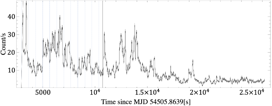
Figure 1: Background subtracted 0.1–15 keV light curve of IGR J00370+6122, acquired in the first XMM-Newton observation with EPIC/PN. The vertical lines indicate the 674 s periodicity.

2.2 Suzaku/XIS

The archival Suzaku data of IGR J00370+6122, in the 0.2–12 keV range, were acquired in 2007 (MJD 54274). Of the four XIS cameras, we utilize the data from XIS0, XIS1, and XIS3, which were operated with 1/4 window mode at that time. The HXD data are not employed, because IGR J00370+6122 was not detected by the HXD. We processed and screened the XIS data with aepipeline 1.1.0. and extracted source and background event with xselect. The source events were accumulated over a circular region with $110^{\prime\prime}$ radius around the source position. The background events were derived from two rectangular regions, both having a size of $180^{\prime\prime}\times 216^{\prime\prime}$ and located at $0^{\circ}.1$ off the source. The RMFs and ARFs were generated using xisrmfgen and xisarfgen in HEASoft, respectively.

2.3 Swift/BAT and Swift/XRT

To improve the orbital ephemeris of IGR J00370+6122, we use its 15–50 keV Swift/BAT daily light curve from 2005 February to 2019 November, provided by the Swift/BAT Hard X-ray Transient Monitor project (Krimm et al., 2013).

IGR J00370+6122 was observed also with the Swift/XRT, 24 times during $\sim 100$ days in 2013 (MJD 56319-56420), and 7 days in 2015 (MJD 57023-57029). These photon-counting-mode data sets, 31 altogether, are also analyzed in the present work. We processed each data set, consisting of 0.2–10.0 keV photons, using xrtpipeline and produced the spectra and light curves using xrtproducts. The on-source events were extracted from a circle of $47^{\prime\prime}$ radius, and the background events from an annulus with the inner and outer radii of $94^{\prime\prime}$ and $141^{\prime\prime}$, respectively.

2.4 The other data sets

The RXTE/PCA archival data, in which in’t Zand et al. (2007) detected the 346-s pulsation, were used to characterize the spectrum of IGR J00370+6122 in an intermediate energy range (7–30 keV). The background and response files are included in the same archive. We ignored ¡8 keV region to avoid Xenon L-edge feature.

The reduced INTEGRAL/ISGRI spectrum was downloaded from the site of High-Energy Astrophysics Virtually ENlightened Sky (HEAVENS), provided by the INTEGRAL Data Centre (ISDC). We selected 17.3–80.0 keV good-quality events that were acquired over 2003–2012 and in an orbital phase interval from -0.1 to 0.1. The background and response matrix were generated also by HEAVENS.

3 Data Analysis and Results

3.1 Orbital intensity variations

As the first attempt of our data analysis, the 15-yr Swift/BAT light curve in 15–50 keV was analyzed for the expected 15.7 d orbital periodicity (in’t Zand et al., 2007; González-Galán et al., 2014), employing the standard epoch-folding method with chi-square evaluation. We used the efsearch software with 32 phase bins, and scanned the trial period from 12 d to 20 d with a step of 0.0007 d. The obtained periodogram is shown in figure 2. A strong peak seen around 15.66 d represents the orbital period, as reported in the previous works. By fitted this peak with a Gaussian, we determined the orbital period as

$$P_{\rm orb}=15.6649\pm 0.0014~{}{\rm d}$$ (1)

where the error refers to 90% confidence level. This $P_{\rm orb}$ is consistent with the previous measurements (in’t Zand et al., 2007; González-Galán et al., 2014), and has a better statistical accuracy, because we used a longer observation span.

Figure 3 is the 15–50 keV Swift/BAT light curve folded at $P_{\rm orb}$, where phase 0 is taken as the periastron time of

$${\rm MJD}\>55084.018$$ (2)

as determined by González-Galán et al. (2014). Thus, the source exhibits a strong orbital intensity variation, and has been detected with the Swift/BAT over a limited orbital phase of about $-0.1$ to 0.25. In addition, the intensity maximum is clearly delayed from the periastron by $\sim 0.05$ orbital cycle, although the delay could be slightly smaller than the previously reported $0.1-0.2$ cycles (Grunhut et al., 2014; González-Galán et al., 2014).

Figure 2: Periodgram of the 15-yr Swift/BAT data, revealing the orbital period. The inset shows an enlargement around the 15.7-d peak.

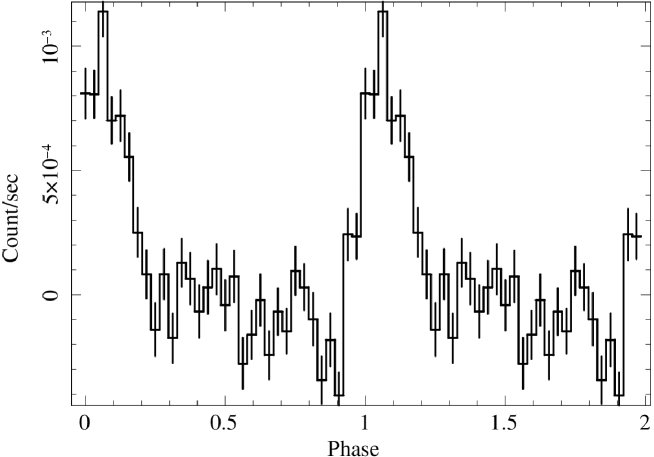
Figure 3: The Swift/BAT data, folded at $P_{\rm orb}$ of equation (1) and shown for two cycles. The epoch of phase zero is set as the periastron time given in González-Galán et al. (2014).

In table 1, we summarize the orbital phases of the individual observations analyzed in the present work, where the three columns for the orbital phase, (1) to (3), employ the three orbital solutions; Grunhut et al. (2014), González-Galán et al. (2014), and the present work. Below, we utilize our own phase values, which are based on $P_{\rm orb}$ of equation (1) and the phase 0 (periastron) epoch of equation (2).

3.2 Search for pulsations

One of the most important objectives of the present study is to confirm that the compact object in IGR J00370+6122 is a magnetized NS powered via mass accretion. Evidently, the best way towards this goal is to detect a periodic source pulsation, at a period that is consistent with, or closely related to, the previously recorded 346-s periodicity. For this purpose, we choose the 1st observation with XMM-Newton, because the source was bright at that time, and exhibited multiple flares (figure 1) which are reminiscent of the case with in’t Zand et al. (2007).

3.2.1 Fourier power spectra

Using the background-subtracted 0.1–15.0 keV EPIC/PN light curve shown in figure 1 from this observation, and employing powspec with a time resolution of 1 s with which we generated the light curve, we calculated a Fourier power spectrum over a frequency range of $4\times 10^{-5}-0.5$ Hz. The result is presented in figure 4 in black, where the abscissa (i.e., the frequency) is shown in a logarithmic scale to better reveal the low-frequency region. The power is normalized so as to become 2.0 when the light curve is dominated by the Poisson white noise. Although a strong red noise component emerges at $\lesssim 1$ mHz, we do not find any preferred periodicity in the analyzed range, including in particular at $\sim 2.9$ mHz which corresponds to 346 s.

As seen in figure 1, the source repeated spiky flares in the 1st half of the observation, and became much quiescent in the 2nd half. Therefore, we next calculated the Fourier power spectra for different time regions of this light curve. Red and blue traces in the same figure are the results for the first 8 ks (i.e., 3–11 ks in figure 1) and the remaining part of the light curve, respectively. The 1–10 mHz frequency regions of these spectra are expanded in the inset to figure 4(left). There, the power is still two orders of magnitude higher than would be expected for a pure Poissonian noise, implying that the red noise extends into these frequencies. Superposed on the red noise, the spectrum from the 1st 8 ks exhibits several noticeable peaks, including the highest one at 1.5 mHz, and the 2nd highest one at 2.9 mHz. As evident from the logarithmic top abscissa of the inset, they are apparently in the 1:2 harmonic ratio, and the 4th harmonic could also be seen at 5.6 mHz. This suggests the presence of a 1.5 mHz periodicity (together with its higher harmonics) in the 1st 8 ks of the data, and the 2.9 mHz feature (possibly the 2nd harmonic) could be identified with the 346-s periodicity.

It is however not easy to tell whether these peaks are real, or just due to fluctuations in the strong red noise. We hence adopt the technique by Israel and Stella (1996), which allows us to evaluate the significance of a suggested periodicity in a power spectrum where strong colored noise is present. It compares the power at a particular target frequency, with the local continuum estimated by averaging the spectrum on both (high-frequency and low-frequency) sides with logarithmically symmetric widths. Employing this technique with the smoothing width of 30 wave numbers, we obtained the results shown in the right panel of Figure 4. The smoothed power spectrum, plotted in blue, roughly follows a power-law function with an exponent of -1.5, which is typical of red noise. The red data points (with linear ordinate), obtained by dividing the raw power spectrum by the smoothed one, are confirmed to closely follow a $\chi^{2}$ distribution with 2 degrees of freedom.

There, we observe a series of prominent peaks, at 1.47, 2.93, 5.62, 9.03, and 11.72 mHz. Within the frequency resolution determined by the data length, their ratios, $1.00:1.99:3.82:6.14:7.97$, are consistent with the (mostly even) harmonic ratios 1:2:4:6:8. Among them, the one at 1.47 mHz, to be identified with the fundamental, is obviously the feature noticed in the left panel, and has a chance-occurrence probability of ${\cal P}_{1}=0.0198$ before correcting for the frequency trials. The highest one at 11.72 mHz, regarded as the 8th harmonic, has a normalized power of 11.7, with the pre-trial probability of ${\cal P}_{8}=3.8\times 10^{-3}$.

Let us suppose that the 1.47 mHz peak appeared due to a chance fluctuation, with a probability ${\cal P}_{1}$. Then, the probability to observe also the highest peak, at a frequency corresponding just to the 8th harmonic, should be ${\cal P}_{1}{\cal P}_{8}=7.5\times 10^{-5}$. Further multiplying the frequency trial number, 121, we finally obtain the overall false alarm probability of $0.9\%$. Considering however the ambiguity in choosing the smoothing width, and uncertainties in treating the harmonics, we conservatively quote a probability of a few percent. We therefore conclude, with a confidence of $>90\%$, that the source showed evidence of 1.47 mHz periodicity, or pulsation with a period of $\sim 680$ s, at least during the 1st 8 ks of the data. Incidentally, the chance probability would further decrease if we consider the simultaneous presence of the 2nd, 4th, and 6th harmonics, but this would be an overuse of the harmonic condition.

3.2.2 Periodogram analysis

Although we have obtained evidence for the 1.5 mHz periodicity, the limited frequency resolution does not allow an accurate period determination. Thus, following a standard procedure in pulsar studies, we next calculated chi-square periodograms using efsearch with 32 bins, over the frequency range of 1–10 mHz corresponding to the inset to figure 4, or equivalently, a period range of 100–1000 s, with a step of 0.1 s. The obtained results are shown in figure 5, where panels (1-a), (2-a), and (3-a) represent the entire data, the 1st 8 ks, and the latter 15 ks, respectively.

In agreement with the power spectra with the strong red noise, the obtained chi-square values are much larger than the degree of freedom, essentially at any period studied here. Furthermore, in panel (2-a) derived from the 1st 8 ks of the data, we observe several prominent peaks, although they are not recognized when we use the entire 23-ks data (panel 1), or those from the latter 15 ks (panel 3). The highest peak at $\sim 675$ s, of which the details are shown in panel (2-b), obviously corresponds to the 1.47 mHz periodicity found with the power spectrum. By fitting this peak with a cubic function, we determined the best period, or the maximum point of the probability distribution, as 674 s. A Gaussian fitting has given the same result. Although it is not straightforward to define the associated error, we conservatively quote a value of $\pm 15$ s, as the half-width at half-maximum of the chi-square peak above the background.

In order to cross-check the result obtained using the normalized power spectrum, the significance evaluation was conducted also using the chi-square periodogram. For this purpose, we Fourier synthesized 1000 fake light curves, in which each Fourier amplitude is set to the square root of the normalized power obtained in the previous subsubsection, whereas the associated Fourier phase is randomized. By analysing the fake light curves in the same way as the actual data, we studied the probability of finding chi-square values, exceeding what was observed (about 1800), at the period of 674 s. As a result, the chance occurrence probability was estimated as about 5%, which is consistent with the evaluation using the normalized power spectrum.

The periodogram in panel (2-a) also reveals several weaker peaks, including one at $\sim 340$ s which can be identified with the 2nd harmonic in our power spectrum. Although the fundamental, which was rather weak in the power spectrum, has become dominant in the periodogram, the difference can be understood in the following way. In the normalized spectrum in figure 4 (right), the power is expressed all relative to the local red-noise intensity, so the fundamental becomes weaker due to the stronger local red noise. In contrast, the fundamental peak becomes prominent in the periodogram, because it sums over all the harmonics from $m=1$ (fundamental) to $m=16$ (the Nyquist frequency for 32 bin), whereas the 340 s peak is a sum over only $m=2,4,..,16$. As a further attempt, we detrended the first 8 ks of the XMM-Newton light curve, using the 5th order polynomial. However, no major changes took place either in the power spectra or the periodograms.

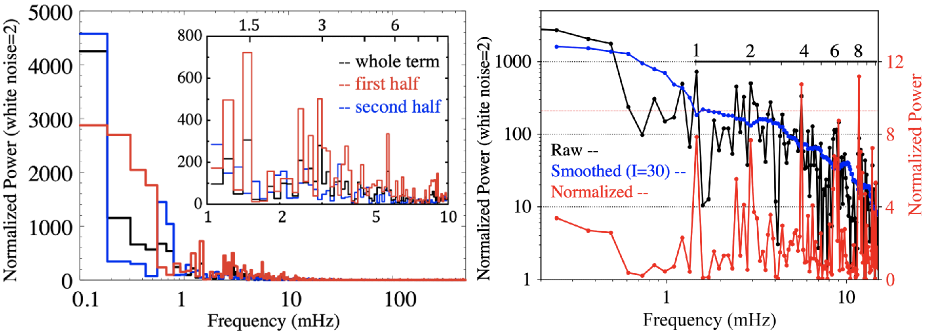
Figure 4: (Left) Fourier power spectra for the whole (black), the first 8 ks (red), and the remaining part (blue) of the XMM-Newton/PN light curve. The abscissa is logarithmic, in order to reveal low-frequency structures. The inset is the enlarged view of the spectra in the 1–10 mHz range, where the logarithmic tick marks at the top abscissa are drawn at multiples of 1.5 mHz. (Right) Evaluation of the power spectrum from the first 8 ks, using the technique by Israel and Stella (1996). The raw spectrum in black (the same as red in the left panel) is averaged over 30 data points, into a smoothed spectrum shown in blue. Both use logarithmic ordinate. The red solid line presents the normalized spectrum, where the raw spectrum is divided by the smoothed one. It refers to the linear ordinate on the right, and the inset abscissa shows the harmonic numbers. The horizontal dashed line in red indicates the 99% confidence level for a single trial.

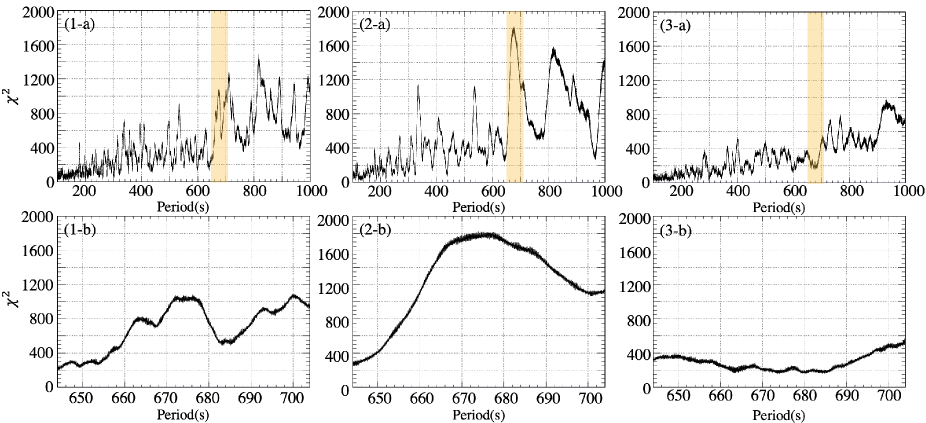
Figure 5: Chi-square periodograms with 32 bins, derived from (1-a) the whole data, (2-a) the first 8 ks, and (3-a) the latter 15 ks. Panels (1-b) to (3-b) expands these periodograms over a period range of 645–705 s.

3.2.3 Folded pulse profiles

For a further confirmation of the results derived so far, we inspected the original light curve in figure 1, and found that sharp intensity minima repeats at about 674 s, as indicated by thin vertical lines over the relevant portion of the data. Therefore, the periodicity is considered to have good coherence. In addition, such sharp intensity drops are likely to arise via geometrical effects (e.g., self eclipse of the emission region) related to the rotation of the compact object (a NS in this scenario). This makes a contrast to the case of flares, which would occur either at a specific rotation phase of the compact star, or in a manner unrelated to the rotation (e.g., caused by quasi-periodic blobs in the stellar winds). Therefore, we regard the 674-s period as a strong candidate for the pulse period of this X-ray source. Its relation to the previously reported 346-s period is considered in subsection 4.1.2.

Figure 6 shows the pulse profile, obtained by folding the 0.1–15.0 keV data from the 1st 8 ks at the period of 674 s.

The pulse profile is rather structured, in a qualitative agreement with the emergence of up to the $m=8$ harmonics in figure 4 (right). In addition, the profile is double-peaked, consisting of a pair of large and small peaks which are about half a cycle apart. This explains why the even higher harmonics are strong in the power spectra (either raw or normalized).

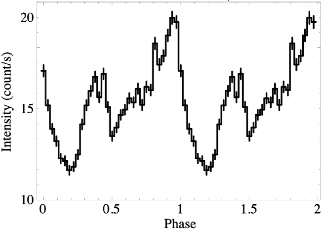
Figure 6: The 0.1–15 keV EPIC/pn data from the 1st 8 ks of the XMM-Newton observation, folded at 674 s.

3.3 Analysis of the brighter spectra

To constrain the nature of the compact object of IGR J00370+6122 from X-ray spectral viewpoints, we analyzed 1-10 keV energy spectra obtained by the XMM-Newton/EPIC, the Suzaku/XIS, and the Swift/XRT. Below, errors and upper limits of the spectral parameters. as well as those on fluxes and luminosities, all refer to 90% confidence levels.

We first analyze the PN/MOS1/MOS2 spectra, acquired in the XMM-Newton observation in the flaring state (figure 1). The data have the highest statistics, and have allowed us to detect the 674-s tentative pulse period. Because the spectra derived from the 1st 8 ks and the latter 15 ks do not show significant differences (except that in the normalization), below we employ the entire data. As presented in figure 7(a) and table 2, a simple power-law model with absorption (phabs * powerlaw) approximately reproduced the spectra, incorporating a rather hard photon index of $\Gamma\sim 1.2$. However, the fit was unacceptable due to residuals at $<2$ keV and $>7$ keV. When we employ a cutoff power-law model instead, the residuals have disappeared and the fit has become acceptable (table 2). The derived photon index is even harder, $\Gamma\sim 0$, and the cutoff energy is obtained as $E_{\rm cut}\sim 3.7$ keV.

The Suzaku/XIS data were obtained for 60 ks in quiescence, when the source was about 40 times fainter than in the flaring-state XMM-Newton observation. The source exhibited small (a factor of $<4$) variability, without significant pulsations. As presented in figure 7(b) and table 2, the time-averaged 1–10 keV XIS spectra were reproduced reasonably well by the simple absorbed power-law model, with a softer photon index of $\Gamma\sim 2$. When we apply the cutoff factor to the power-law continuum, the fit has been improved, with a decrease in chi-square by about 30, and the cutoff energy has been constrained as $E_{\rm cut}\sim 3$ keV (table 2 for details).

The Swift/XRT data sets have a typical exposure of a few kiloseconds each. Although some of these data sets, particularly those when the source is active, showed factor 3–10 intensity variations within each, we again analyze the spectra which are averaged over individual observations. Among the 31 data sets altogether, nine (all acquired in flaring activity and near the periastron) have statistics which are high enough for the spectral studies. As summarized in table 2, these 9 spectra have all been reproduced successfully by the absorbed power-law model. Figure 7(c) shows the brightest five spectra.

In figure 7(c), we observe a spectral change with a “harder when brighter” trend; the spectrum becomes harder ($\Gamma$ gets smaller) when the source flux becomes higher. For a further confirmation of this property, figure 8 shows a scatter plot between $\Gamma$ and the 1–10 keV flux, obtained with the XMM-Newton/EPIC, the Suzaku/XIS, and the Swift/XRT (the 9 data sets). Thus, the “harder when brighter” property is clearly confirmed.

As in table 2, the absorbing column density $N_{\rm H}$ was relatively constant at about $1\times 10^{22}$ cm^-2, when the spectra from the different instruments are fitted individually with a power-law continuum. Since the high-statistics XMM-Newton spectra (ObsID=501450101) require a cutoff power-law continuum and a lower $N_{\rm H}$ value, the actual absorption column density might be at around $0.7\times 10^{22}$ cm^-2.

3.4 Analysis of the fainter spectra

We have so far analyzed 11 spectra, one from XMM-Newton, another from Suzaku, and 9 from the Swit/XRT. We still have one more XMM-Newton data set (the 2nd observation) when the source was very faint and was only in the MOS2 field-of-view, and 22 Swift/XRT spectra acquired at orbital phases rather away from the periastron. Although these data would not have statistics high enough to constrain the spectral properties, they are still useful when we study how the flux depends on the orbital phase. In dealing with these data, we fitted simultaneously the source+background spectrum and the background spectrum, because some data bins would become negative if we directly subtracted the background. The source spectrum was modeled by a simple absorbed power-law, with $\Gamma=2.06$ and $N_{\rm H}=1.26\times 10^{22}$ cm^-2 both fixed, referring to the Suzaku/XIS determinations. The background spectrum was derived from an outer region in the same detector, and was modeled by an unabsorbed power-law, with the photon index fixed at $\Gamma=0.20$ for the XMM-Newton/EPIC spectrum and $\Gamma=0.64$ for those with the Swift/XRT. In each spectral fitting, only the normalizations of the source and background components were set free. The fit goodness was evaluated with the Poisson statics (C-stat in XSPEC, Cash, 1979), instead of the chi-square criterion.

In the 2nd XMM-Newton observation (ObsID 0742800201), with a net exposure of 11 ks, we detected only 26 source+background events, and 13 events in the background region. From these, we obtained a 1–10 keV flux of $(8^{+5}_{-4})\times 10^{-14}$ erg cm^-2 s^-1, which corresponds to a luminosity of $(1.1^{+0.7}_{-0.5})\times 10^{33}$ erg s^-1 at 3.4 kpc. Similarly, by analyzing the fainter 22 Swift/XRT spectra in this way, we positively detected the source in 17 observations, and derived upper limits in the remaining 5 cases. In all of them, the 1–10 keV luminosity was $\lesssim 10^{34}$ erg s^-1. The derived luminosities (including the upper limits) are utilized later in our examination of the orbital luminosity modulation.

Figure 7: Model fitting results to the spectra of IGR J00370+6122, presented in the $\nu F\nu$ form. (a) The EPIC MOS1 (black), MOS2 (red), and PN (green) spectra, obtained in the flaring-state XMM-Newton observation, and fitted simultaneously with an absorbed power-law model. The middle and bottom panels show residuals from the power-law fit and the cutoff power-law fit, respectively, both with absorption. (b) The Suzaku XIS0 (black), XIS1(red), and XIS3 (green) spectra, fitted simultaneously with an absorbed power-law model. The fit residuals are given in the bottom panel. (c) The brightest 5 spectra from the Swift/XRT, fitted individually by an absorbed power-law model. (d) Combined spectra with the RXTE/PCA (black) and the INTEGRAL/ISGRI (red). They were obtained both near the periastron, but not simultaneous.

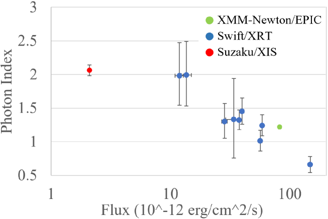
Figure 8: A Scattered plot between the photon index (from the power-law fit) and the 1–10 keV flux. Data points refer to those presented in Table 3.4, i.e., relatively bright data where the spectral shapes have been constrained.

Results of the spectral fitting, using the absorbed power-law and cutoff power-law models. Instruments ObsID Flux^∗ $N_{\rm{H}}$ ($10^{22}$ cm²) $\mit\Gamma$ $E_{\rm{cutoff}}$ $\chi^{2}$/d.o.f RXTE 91061010101^† 220 9.1$\pm$0.3 2.14$\pm$0.02 – – XMM-Newton 0501450101^‡ 83.50 1.16 1.22 – 1558.09/273 0501450101^§ 79.82${}^{+2.74}_{-2.64}$ 0.62${}^{+0.03}_{-0.03}$ 0.05${}^{+0.06}_{-0.06}$ 3.70${}^{+0.19}_{-0.17}$ 316.79/272 Suzaku 402064010 2.08${}^{+0.28}_{-0.25}$ 1.29${}^{+0.11}_{-0.11}$ 2.06${}^{+0.08}_{-0.08}$ – 193.25/147 402064010^§ 1.97${}^{+0.53}_{-0.41}$ 0.67${}^{+0.21}_{-0.20}$ 0.50${}^{+0.47}_{-0.47}$ 2.79${}^{+1.19}_{-0.65}$ 161.62/146 Swift 00032620005 58.70${}^{+1.88}_{-2.00}$ 1.35${}^{+0.23}_{-0.21}$ 1.24${}^{+0.16}_{-0.15}$ – 84.32/78 – 00032620009 39.92${}^{+1.63}_{-1.69}$ 1.45${}^{+0.29}_{-0.26}$ 1.45${}^{+0.20}_{-0.19}$ – 58.47/62 00032620013 11.92${}^{+0.91}_{-0.95}$ 2.09${}^{+0.84}_{-0.73}$ 1.98${}^{+0.49}_{-0.44}$ – 15.67/14 00032620015 13.62${}^{+1.36}_{-1.28}$ 2.90${}^{+0.90}_{-0.79}$ 1.99${}^{+0.50}_{-0.46}$ – 18.90/19 00032620019 56.75${}^{+2.11}_{-2.20}$ 0.82${}^{+0.19}_{-0.17}$ 1.01${}^{+0.16}_{-0.15}$ – 68.47/76 00032620028 34.04${}^{+5.75}_{-4.97}$ 1.88${}^{+1.02}_{-0.89}$ 1.33${}^{+0.61}_{-0.57}$ – 7.77/13 00032620029 28.47${}^{+1.42}_{-1.50}$ 1.96${}^{+0.51}_{-0.45}$ 1.30${}^{+0.27}_{-0.25}$ – 39.92/35 00032620030 148.48${}^{+4.31}_{-4.47}$ 1.03${}^{+0.18}_{-0.16}$ 0.66${}^{+0.12}_{-0.12}$ – 114.42/129 00032620031 37.79${}^{+1.15}_{-1.21}$ 1.32${}^{+0.20}_{-0.18}$ 1.32${}^{+0.15}_{-0.14}$ – 58.35/88

Unabsorbed fluxes in 1–10 keV (3–20 keV for the RXTE/PCA data), in units of $10^{-12}$ erg s^-1 cm^-2.
Parameters refer to in’t Zand et al. (2007) for 3-20 keV.
Fitting results with the cutoff power-law model.

3.5 High-energy spectral properties in bright phases

To characterize the spectrum at higher energies when the source is near the periastron and is hence bright, we analysed the RXTE/PCA (10–30 keV) and INTEGRAL/ISGRI (17.3-80 keV) data. The former was derived from standard data products for ObsID=91061-01-01-01, which caught a flaring activity at an orbital phase of an orbital phase of $\sim$0.05 (or $\sim$0.14 in our phase definition in Table 1) and enabled the detection of the 346-sec period (in’t Zand et al., 2007). The utilized INTEGRAL/ISGRI data cover a 10-year period of 2003–2012, but we selected the events only in the orbital phase interval from –0.1 to 0.1 where the source is significantly bright in figure 3. The RXTE/PCA and INTEGRAL/ISGRI spectra were fitted with a single power-law function without absorption. The fit is simultaneous, except the spectral normalization which is allowed to take separate values between the two spectra considering that they are not simultaneous. As shown in figure 7(d), the fit was successful with a reduced chi-square of 0.99, and gave a flat continuum with a photon index of $2.09\pm 0.04$. We also tried a cutoff power-law fit, in order to constrain a possible spectral turn-over which is observed in many other HMXBs. However, the fit (which was already acceptable) did not improved significantly, and a 90% confidence limit of $E_{\rm cut}>38.6$ keV was derived. Thus, the 10–80 keV spectrum of IGR J00370+6122 can be explained by a $\Gamma\sim 2.1$ power-law without significant high-energy cutoff.

4 Discussion

4.1 The nature of the compact object in IGR J00370+6122

In order to better understand the nature of the compact component in the HMXB IGR J00370+6122, we analyzed various X-ray archival data, obtained with the 6 X-ray instruments onboard altogether 5 missions. These data sets differ in many attributes such as the sensitivity, energy range, observation epoch, time length, orbital-phase coverage, and the source intensity during the observation. Their comprehensive analysis has enabled us to deepen our understanding of this object. Below, we summarize the obtained results from the timing and spectral aspects.

4.1.1 Timing results: orbital intensity variations

Our analysis of the 15–50 keV Swift/BAT data, covering a 15 yr period of 2005–2019, yielded the following three results. First, the orbital period has been refined as in equation (1). Second, as already reported by in’t Zand et al. (2007), the orbit-folded light curve in figure 3 shows a strong orbital modulation, that the X-ray emission is strongly enhanced over a limited orbital phase from $-0.1$ to 0.2. Finally, the same figure reveals a slight ($\sim 0.05$ cycle) delay of the X-ray intensity maximum from the periastron passage, in broad agreement with Grunhut et al. (2014) and González-Galán et al. (2014).

Although the second result above is of importance, the limited Swift/BAT sensitivity hampers us to infer from figure 3 to what extent the source gets dim when it is away from the periastron. To understand this issue, in figure 9 we plot all the flux measurements from the present study, except those with the Swift/BAT, as a function of the orbital phase. Thus, away from the periastron phases, the source has been found to decline to extreme low luminosities, down to $\sim 10^{32}$ erg s^-1, almost by 3 orders of magnitude from the periastron phases. This behavior is likely to repeat regularly each orbital cycle, because it is consistently indicated by the relatively dense sampling with the Swift/XRT, as well as by the Suzaku and the 2nd XMM-Newton observations. In addition, we find a hint of a rather abrupt luminosity drop at an orbital phase of $\sim 0.3$, and possibly a quick return at a phase of $\sim 0.95$. Later, we try to theoretically explain this behavior.

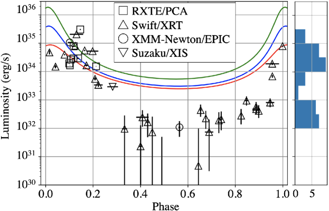
Figure 9: Orbital variations of the X-ray luminosity of IGR J00370+6122. The data points of Swift/XRT, XMM-Newton/EPIC and Suzaku/XIS are from the present analyses, while RXTE/PCA ones are from in’t Zand et al., 2007. Three solid curves are theoretical predictions (see text), calculated for the stellar mass/eccentricity of (red) $22~{}\MO/0.48$, (blue) $15~{}\MO/0.56$, and (green) $8~{}\MO/0.56$, referring to Grunhut et al. (2014), González-Galán et al., 2014 and Hainich et al., 2020, respectively. The right histogram shows the distribution of the measured luminosities excluding upper limits.

4.1.2 Timing results: the possible pulse detection

To reconfirm the pulsation that was detected only once in the past by the RXTE/PCA, we searched for a pulsation using the 2008 XMM-Newton data, which are suitable for this purpose because the object was rather bright and flare active as in the RXTE observation, and the data have a longer exposure (23 ks vs 4 ks). As a result, a candidate period has been discovered at $674\pm 15$ s.

in’t Zand et al. (2007) in fact found, in their RXTE periodogram, not only the 346 s peak which they favor, but also a broad enhancement at about 700 s (which is higher than the 346 s peak) and 550 s. Therefore, the two observations consistently prefer three common periods; 340-346 s, $\sim 550$ s, and 674-700. Although the nature of the $\sim 550$ s enhancement is unclear, the other two periods can most naturally be regarded as the the fundamental and the 2nd harmonic, as we already argued repeatedly. If the folded pulse profile is mildly time variable, the major and minor peaks in figure 6 could sometimes have comparable intensities, to make the pulse period appear to be $\sim 340$ s. In fact, the X-ray pulsar Vela X-1 was first thought to have a pulse period of about 141 s, but the period was later revised as 283 s (Mcclintock et al., 1976).

4.1.3 Spectral results

Next, the energy spectral analyses were performed to characterize IGR J00370+6122 from spectral viewpoints. The 1-10 keV energy spectra obtained by the XMM-Newton/EPIC, the Suzaku/XIS, and the Swift/XRT were approximately represented by an absorbed power-law model. Furthermore, a mild spectral cutoff with $E_{\rm cutoff}=3-4$ keV, together with a very hard spectral slope with $\Gamma=0-0.5$, are indicated by the XMM-Newton spectrum, and by the Suzaku data to a lesser extent. The absorption column density was stable at $N_{\rm H}\sim 1\times 10^{22}$ cm^-2. Since the optical companion, BD+60 73, has an optical extinction of $A_{\rm v}=2.39$ (González-Galán et al., 2014; Hainich et al., 2020), the Galactic line-of-sight column is estimated as $N_{\rm H}\sim(5-6)\times 10^{21}$ cm^-2, which is consistent with the Galactic coordinates of IGR J00370+6122, $(\ell,b)=(121^{\circ}.2,-1^{\circ}.5)$, and its distance. Thus, the observed $N_{\rm H}$ is likely to be a mixture of about equal Galactic and circum-source contributions. Analyzing the 3–20 keV RXTE/PCA spectrum with an absorbed power-law model, in’t Zand et al. (2007) derived $N_{\rm{H}}\sim 10^{23}$ cm^-2 (table 3.4), which is an order of magnitude higher than those we have obtained. This discrepancy probably arose because the intrinsic spectral curvature was mimicked by the strong absorption, when the RXTE/PCA spectrum above 3 keV was fitted with a single power-law.

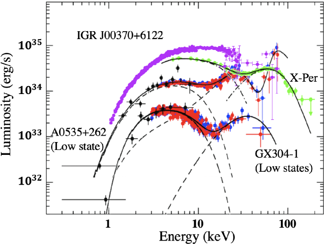
Figure 10: A combined spectrum with XMM-Newton/EPIC, RXTE/PCA and INTEGRAL/ISGRI of IGR J00370+6122 is compared with those of X Persei, A0535+26 and GX304-1 adapted from Doroshenko et al. (2012), Tsygankov et al. (2019a) and Tsygankov et al. (2019b). For IGR J00370+6122, the XMM-Newton/MOS2, PN, RXTE/PCA and INTEGRAL/ISGRI spectra are renormalized in reference to the XMM-Newton/MOS1 spectrum.

4.1.4 Identification of the compact object in IGR J00370+6122

Even though the evidence for the 674-s pulsation gives a strong support to the argument for a magnetized NS in this system, we are still left with a few percent probability that the detection is false. In addition, the pulsation was detected only from a limited portion of the XMM-Newton observation. Similarly, the evidence for pulsation had been obtained only once, out of a number of past observations. Therefore, we need to carefully examine whether our interpretation can be supported from other pieces of evidence.

Starting our examination from a basic viewpoint, the compact object in IGR J00370+6122 must be either a white dwarf, a black hole (BH), or a NS. The maximum luminosity of $\sim 10^{35}$ erg s^-1 and the 674-s pulsation (assuming it to be real) are both explicable in terms of a white dwarf. However, it would be extremely unlikely that a white dwarf ever formed a binary with a massive star. The observed spectrum, with weak or no emission lines, also disagrees with line-rich thermal spectra from accreting white dwarfs. Therefore, the white dwarf scenario can be readily ruled out.

Let us next consider a possibility that the compact star is a BH. In fact, the observed violent variability and the relatively hard spectra both broadly agree with those of accreting BHs. If so, however, the luminosity of this object, $10^{35}$ erg s^-1 when it is bright, would translate to 0.02% of the Eddington luminosity for a typical BH mass of $5~{}\MO$. Then, the BH would have to be in the low/hard state, wherein the spectrum from a few keV to a few tens keV should be approximated by a $\Gamma\sim 1.7$ power law, accompanied by a clear cutoff with $E_{\rm cutoff}=50-150$ keV (e.g., Makishima et al., 2008). The observed spectrum of IGR J00370+6122 is clearly distinct, harder than this in $<10$ keV, and softer but possibly less curved in $>10$ keV. Thus, the compact object cannot be considered as a BH, either.

As a result, we are left with the sole option that the compact object is a NS. In this case, we still have to tell whether the NS is strongly magnetized with the MFs $B\gtrsim 10^{12}$ G, or has relatively weak MFs as $B\lesssim 10^{9}$ G. Clearly, the former is favored for a few reasons. First, as an old stellar population, weak-field NSs form binaries predominantly with low-mass stars, and rarely with massive ones. (Probably IGR J00370+6122 is located on the Perseus arm.) Second, the former type of objects often exhibit flare-like variations like those seen in IGR J00370+6122 on time scales of minutes, whereas the latter objects, when dim, vary randomly on times scales of minutes to hours, but more continuously, typically with a relative amplitude of $\sim 20\%$ (e.g., Takahashi et al., 2011). Finally, the spectrum of IGR J00370+6122 is very similar to those of binary X-ray pulsars (see next subsection), whereas distinct from those of weak-MF NSs (e.g., Ono et al., 2017) which are more similar to those of BHs in the low/hard state. Therefore, independently of the 674-s periodicity, our comprehensive study supports the presence of a high-MF NS in IGR J00370+6122.

4.2 Comparison with the known binary X-ray pulsars

Taking it for granted that the compact object in IGR J00370+6122 is a magnetized NS, our next task is to compare it with the known binary X-ray pulsars, particularly those with low luminosities, to understand its properties and behavior as a mass-accreting NS.

4.2.1 General similarities

We have successfully quantified the 1–10 keV spectra of IGR J00370+6122  over a rather wide luminosity range as seen in figure 7, and found that the photon index becomes harder from 2 to $<1$ as the luminosity increases from $3\times 10^{33}$ to $2\times 10^{35}$ erg s^-1 (figure 8). This spectral behavior, “harder when brighter”, and the very hard photon index of $<1$, agree with the properties observed from nine Be-type X-ray pulsars when they are $<0.1$ times the Eddington luminosity (Reig & Nespoli 2013). This similarity provides yet another supporting evidence that IGR J00370+6122 is an accreting magnetized NS. The “harder when brighter” trend, consistently observed from these low-luminosity pulsars (including IGR J00370+6122), may be explained as a spectral hardening caused by an increase of the inverse-Compton scattering probability, in response to the increase in the accretion rate (Ballhausen et al., 2017).

We find several additional similarities between IGR J00370+6122 and Be-type pulsars. These include the large orbital intensity changes (figure 9), the small but significant difference between the peak-brightness and periastron phases (figure 3), and the weakness of iron-K emission line (figure 7). Considering further the lack of a circumstellar disk (Reig et al., 2005) in the primary BD+60 73, its stellar winds may be somewhat anisotropic, and denser along equatorial directions of its rotation.

As seen so far, the magnetized-NS interpretation is supported, not only via the elimination argument, but also by general similarities seen between IGR J00370+6122 and the known binary X-ray pulsars (particularly of Be companions).

4.2.2 Magnetic fields and spin periods

Using the RXTE/PCA and INTEGRAL/ISGRI data (though not simultaneous), we have found that the high-energy spectrum of IGR J00370+6122 extends up to 80 keV with a photon index of $\Gamma\sim 2.2$, without noticeable cutoff. Combined with the information below 10 keV from XMM-Newton, Suzku, and Swift, the X-ray spectrum of IGR J00370+6122 is hence found to keep a rather flat shape over nearly two orders of magnitude in energy. Actually, the constraint of $E_{\rm cutoff}>38.6$ keV derived for IGR J00370+6122 is considerably higher than the values of $E_{\rm cutoff}=5-10$ keV measured from binary X-ray pulsars at a typical luminosity of $\sim 10^{37}$ erg s^-1. This difference may be attributed to the very low luminosity of IGR J00370+6122, $\sim 1\times 10^{35}$ erg s^-1, or 0.1% of the Eddington luminosity for a NS with 1.4 $M_{\odot}$, even though it refers to the brightest phase near the periastron.

To examine the above possibility, we compare in figure 10 the broad-band spectrum of IGR J00370+6122 with those of three binary X-ray pulsars with comparable low luminosities, all having Be-type optical companions. One is the nearby binary X-ray pulsar X Persei, which has a persistently low luminosity (Doroshenko et al., 2012; Tsygankov et al., 2019a, b; Yatabe et al., 2018). The other two are typical recurrent Be-type transients, A0535+26 and GX $304-1$, which were recently observed in a very X-ray dim phase during a decay phase of their outbursts (Ballhausen et al., 2017; Tsygankov et al., 2019b). Thus, the most outstanding spectral property common to the four objects is the hard X-ray continua that extend with a flatter shape to higher energies, than those of more luminous accreting pulsars which strongly turn over at $\gtrsim 20$ keV. Therefore, the flat spectrum of IGR J00370+6122 may be explained, at least partially, as a property which is common to dim X-ray pulsars, even though its mechanism is unclear at present.

Another noticeable property in figure 10, which is particularly prominent in A0535+26 and GX $304-1$, is a two-hump structure of the spectrum, with two peaks at a few keV and a few tens keV, as already pointed out by Tsygankov et al. (2019a) and Tsygankov et al. (2019b). (In A0535+26, another sharp dip at 50 keV is due to the CRSF; Terada et al., 2007). This two-hump structure is possibly present in X Persei and in IGR J00370+6122 as well, but less visible. Among the three comparison objects, A0530+26 and GX $304-1$ have surface MFs of $B\sim 4.5\times 10^{12}$ G and $\sim 5.5\times 10^{12}$ G, respectively, as measured securely with their CRSFs. In contrast, X Persei has a considerably stronger dipole MF of $B\sim$10¹⁴ G, as estimated through the GL79 modeling (Introduction; Yatabe et al., 2018) which has been verified and calibrated quantitatively using long-term MAXI observations (Sugizaki et al., 2015; Takagi et al., 2016; Sugizaki et al., 2017, 2020). Then, the closer resemblance of the IGR J00370+6122 spectrum to that of X Persei, than to those of the two recurrent transients, suggest that IGR J00370+6122 also has a MF of $>10^{13}$ G, as already suggested by Grunhut et al. (2014). This inference is also supported by an empirical positive dependence of $E_{\rm cutoff}$ on the CRSF energy (Makishima et al., 1999); this dependence may be explained theoretically in terms of cyclotron resonance cooling in the accretion column which will shift to higher energies for stronger MFs.

Interestingly, the three comparison objects in figure 10 have relatively long spin periods on the order of 100 s or longer. Other examples of low-luminosity pulsars with hard flat spectra and very long periods include 4U 0114+65 (with a period of 9340 s), 4U 1954+317 ($\sim 2\times 10^{4}$ s), and 4U 2206+54 (5540 s). In contrast, the Be pulsars with fast rotation, 4U 0115+63 (3.6 s) and X0331+53 (V0332+53; 4.4 s), show rather softer spectra when they are dim at $\lesssim 10^{34}$ erg s^-1 (Wijnands & Degenaar 2016). Therefore, an X-ray pulsar with a low luminosity and a hard continuum spectrum tends to have a long spin period. This empirical tendency suggests IGR J00370+6122 to have a long spin period as well, and reinforces the case for the 674-s pulsation.

4.3 The luminosity change along the orbit and magnetic propeller effects

As discussed in section 4.1.1, we have found that the luminosity of IGR J00370+6122 changes along the orbit by a large dynamic range reaching three orders of magnitude (figure 9). We further notice an abrupt luminosity drop at the orbital phase $\sim 0.3$, from $\sim 4\times 10^{33}$ to $\sim 1\times 10^{32}$ erg s^-1, and possibly a reversal at the orbital phase $\sim 0.95$. Let us numerically examine whether this behavior can be explained by a standard scenario of the wind-capture accretion.

Presuming that the NS in IGR J00370+6122 is powered by capturing the stellar winds from the massive primary, we employ a simple Hoyle-Lyttleton accretion picture, taking into account the orbital phase dependence of the wind capture rate (Wind-Rose effect, Natalya & Lipunov 1998). In this picture, the mass accretion rate $\dot{M}_{\rm acc}$ onto the NS is assumed as

$$\dot{M}_{\rm acc}=\frac{1}{4}\left(\frac{R_{\rm cap}}{r}\right)^{2}\left(\frac{v_{\rm rel}}{v_{\rm w}}\right)\dot{M}_{\rm w}~{}.$$ (3)

Here, $r$ is the distance of the NS from the primary star, $\dot{M}_{\rm w}$ is the primary’s wind mass loss rate, $v_{\rm rel}$ is the relative velocity between the NS star and the local stellar wind, $v_{\rm w}$ is the stellar-wind velocity at the position of the NS, and $R_{\rm cap}$ is the gravitational wind-capture radius defined as

$$R_{\rm cap}=\frac{2GM_{\rm NS}}{v_{\rm rel}^{2}}~{},$$ (4)

where $G$ is the gravitational constant, and $M_{\rm NS}$ is the NS mass. In the calculation, we assume the stellar wind from the primary to be isotropic, and utilize the wind velocities numerically given in table A.7 of Hainich et al. (2020) as a function of the distance from the star, which is assumed to have a radius of 16.5 $\RO$. We adopt $\dot{M}_{\rm acc}=3\times 10^{-8}~{}\MO$ yr^-1 from Hainich et al. (2020). The orbital motion of the NS is calculated using the orbital period of equation (1), together with three cases for the primary’s mass and the orbital eccentricity as described in the caption. The X-ray conversion factor is set to be unity, i.e., the gravitational energy gained via accretion is all converted to the radiation, assuming a NS radius of 12 km and a NS mass of 1.4 $\MO$. Any other complex effects (e.g., a photoionization of the stellar wind by the X-ray) are not taking into account in this calculation.

The X-ray luminosity changes calculated in this way are superposed in figure 9 on the observed data, where the phase 0 is aligned with the periastron passage time of equation (2). The model curves have the peak at an orbital phase of 0.02–0.03, This is because $v_{\rm rel}$ becomes minimum right after the periastron passage. In contrast, the observed luminosity peak is more delayed from the periastron epoch. As already mentioned in subsection 4.2, this discrepancy may be attributed to some anisotropy of the stellar wind properties. We do not discuss this issue any further.

The calculated orbital modulation of the luminosity is thus 1.5 to 2.5 orders of magnitude, which arises mainly due to changes in $v_{\rm rel}$, hence those in $R_{\rm cap}$, along the eccentric orbit. These are significantly smaller than the observed dynamic range (3 orders of magnitude). Even when a systematic normalization adjustment (due, e.g., to an estimation error of $\dot{M}_{\rm w}$) is allowed between the observation and calculation, this discrepancy is too large to be attributed to systematic errors of any of the assumed parameters. For example, to explain the observation, the orbital eccentricity would have to be extremely large as $>0.9$, in contradiction to the optical observations. Alternatively, the stellar winds should have to be accelerated to have a twice higher velocity at the apastron than at the periastron; this is also unlikely. A still more important point is that none of these ideas would be able to explain the markedly dim phase interval observed between the orbital phases of $\sim$ 0.3 and $\sim$ 0.95. To explain this phenomenon, we need to invoke some additional effects, in addition to the simple Hoyle-Lyttleton accretion scenario.

One possibility is the X-ray photoionization of the stellar winds, which may cause large luminosity changes along the orbit (Bozzo et al., 2020). To evaluate this effect, we calculated the ionization parameter $\xi$ at the periastron. Among the three conditions considered in the present work, the shortest distance between the primary’s surface and the NS is $r\sim 10~{}\RO$, where the stellar-wind density becomes $n\sim 10^{11}$ cm^-3 (Hainich et al., 2020). The maximum X-ray luminosity is $L\sim 10^{36}$ erg s^-1. These conditions yield $\xi\equiv L/nr^{2}\sim 20$ erg s^-1 cm^-1. Therefore, the photoionization would not work sufficiently in IGR J00370+6122  because it is considered inefficient even in Vela X-1, which has a much higher value of $\xi\sim 10^{4}$ (Bozzo et al., 2020). Even if the photoionization ever worked, it would produce two sharp peaks in the orbital X-ray light curve (Bozzo et al., 2020), one preceding and the other following the periastron, with a relatively reduced luminosity in between. The observed behavior of IGR J00370+6122 is opposite, showing an abrupt luminosity increase over an orbital phase near the periastron between $\sim$0.3 and 0.95. Therefore, we conclude that the photoionization effect cannot explain the light curve of this system, and that other explanations must be sought for.

The observed long pulse period and the low X-ray luminosity make IGR J00370+6122 very reminiscent of X-Persei, which has $B\sim 10^{14}$ G (see section 1). Similarly, comparing three fundamental radii of accreting NS binaries, i.e. accretion, corotation, and Alfvén radii, Grunhut et al. (2014) argued that IGR J00370+6122  possibly has a strong magnetic field of $\sim 10^{15}$ G. If so, we naturally expect the operation of so-called propeller effect, which has actually been observed in some NS binaries (e.g., Asai et al., 2013; Tsygankov et al., 2016). In short, the gravitationally captured material can accrete onto the NS (accretion mode) when the matter density is high and hence the Alfvén radius is smaller than the co-rotation radius. When the matter density decreases to below a certain threshold, the pulsar magnetosphere will expand beyond the co-rotation radius, to prevent the direct mass accretion onto the NS. The latter is often called “propeller mode”, because the rotating magnetosphere would expel the matter off the NS. This picture can explain the very low luminosity away from the periastron as a continued propeller-mode phase, and the observed luminosity jumps as the epochs of transitions between the accretion and propeller modes. This inference is strengthened by the histograms given on the right side of figure 9, which indicate that the luminosity takes a bimodal distribution, with a gap between $\sim 10^{33}$ and $\sim 10^{34}$ erg s^-1.

Let us apply the propeller effect modeling to the case of IGR J00370+6122. If the transition between the accretion mode and the propeller mode takes place at an X-ray luminosity $L_{\rm X}$, where the gravitational pull and the magnetic pressure are balanced, the dipolar MF strength $B$ (expressed by its value on the surface) is given as

$$B \sim 5.7\times 10^{13}\zeta^{-\frac{7}{4}}\left(\frac{L_{\rm X}}{10^{33}\rm{\ erg\ s^{-1}}}\right)^{\frac{1}{2}}\left(\frac{P}{10^{3}\;\rm{s}}\right)^{\frac{7}{6}}\quad\rm{G}$$ (5)

where $P$ is the spin period and $\zeta\sim$1 is a numerical factor (Makishima, 2016). Employing $P=674$ s and the mode transition luminosity as $\sim 2\times 10^{33}$ erg s^-1 from figure 9, we obtain $B\sim 5\times 10^{13}$ G. As clear from the above equation, this high value of $B$ is a direct consequence of the long spin period. In addition, the very low luminosity of IGR J00370+6122 can be explained naturally as a consequence of magnetic inhibition of the wind capture process (Yatabe et al., 2018). Thus, IGR J00370+6122, like X Persei, is thought to have a dipole MF which is considerably higher than those of typical binary X-ray pulsars, and is even comparable to those of magnetars. This inference agrees with the suggestion derived in subsection 4.2 based on our broadband spectral comparison. In this case, the CRSF should appear around 600 keV, which would be hard to detect. This is consistent with an apparent lack of the CRSF in the 1–80 keV spectrum of figure 10.

We have so far invoked the GL79 torque equilibrium theory and a strong MF to explain the low luminosity and the slow spin period. The application of the GL79 scheme is supported by a series of successful calibrations (see Introduction), and the case of the two Be-type pulsars, 4U 0115+63 (3.6 s pulse period) and X0331+35 (V0332+53, 4.4 s). In a declining phase of their outbursts, these objects showed a clear luminosity drop, to be interpreted as due to the propeller effect (Tsygankov et al., 2016), at luminosities of $1.4\times 10^{36}$ erg s^-1 and $2.0\times 10^{36}$ erg s^-1, respectively. Then, equation (5) gives $B=2.5\times 10^{12}\zeta^{-\frac{7}{4}}$ G for 4U 0115+63 and $B=2.5\times 10^{12}\zeta^{-\frac{7}{4}}$ G for X0331+53, which agree very well with their surface MF strength measured with the CRSF, $1.2\times 10^{12}$ G and $3.0\times 10^{12}$ G, respectively (Makishima, 2016). Of course, some reservations may be needed, because the presence of a stable accretion disk, assumed in the GL79 scheme, may not necessarily be applicable to the present object. If, instead, so-called quasi-spherical accretion (QSA) (Shakura et al., 2012, 2014) takes place, the required MF strength would be reduced to $\sim 10^{12}$ G (e.g., Sanjurjo-Ferrrín et al., 2017). For example, the SFXT IGR J11215-5952 is characterized by a persistently low luminosity, a long spin period, and periodic flares at periastron (Sidoli et al., 2020 and references therein), and is very reminiscent of IGR J00370+6122. Sidoli et al. (2020) tried to explain its behavior using the QSA framework. Considering however the richer observational verification of the GL79 scheme than that of the QSA, and the independent evidence from the harder and flatter spectral continuum, we would still favor the strong-MF interpretation of IGR J00370+6122.

This conclusion will be strengthened if follow-up observations of IGR J00370+6122 in the future confirms the rapid luminosity jump at the orbital phases $\sim 0.3$ and $\sim 0.95$.

5 Conclusion

By analyzing archival X-ray data of IGR J00370+6122 obtained with XMM-Newton, Suzaku, Swift, RXTE, and INTEGRAL, we have obtained the following results.

1. The orbital period has been refined. Near the periastron, the source brightens up to $\sim 2\times 10^{35}$ erg s^-1, and often exhibits flaring activity. The luminosity peak is delayed by $\sim 0.05$ orbital cycles from the periastron passage.

2. From the 1st 8 ks of the 2008 XMM-Newton observation made near periastron, a possible periodicity was detected at 674 s. This strongly suggests that the compact object is an accreting magnetized NS rotating rather slowly at this period. Because the pulse profile folded at 674 s is double peaked, the previously reported 346 s period could be half (or twice in frequency) that observed in the present work.

3. Through the analysis of 1–10 keV spectra obtained with 3 instruments, the “harder when brighter” trend has been confirmed. This makes IGR J00370+6122 similar to known binary pulsars accreting at low luminosities.

4. A combined 10–80 keV spectrum can be described by a single power-law with $\Gamma\sim 2.2$ without noticeable cutoff. Its similarity to the spectrum of X Persei empirically suggests that IGR J00370+6122 has a considerably higher MF than ordinary X-ray pulsars.

5. Away from the periastron, the luminosity has been found to decrease by 3 orders of magnitude, down to $\sim 1\times 10^{32}$ erg s^-1, involving abrupt luminosity jumps. These can be explained by the magnetic propeller effect, and a MF of $5\times 10^{13}$ G is derived.

This work was supported by JSPS KAKENHI Grant Number 19J13685.

References

- Asai et al. (2013) Asai, K., et al. 2013. The Astrophysical Journal, 773, 2, 117
- Ballhausen et al. (2017) Ballhausen, R., et al. 2017. A&A, 608, A105
- Bozzo et al. (2020) Bozzo, E., Ducci, L., & Falanga, M. 2020. Monthly Notices of the Royal Astronomical Society, 501, 2, 2403–2417
- Bozzo et al. (2008) Bozzo, E., Falanga, M., & Stella, L. 2008. The Astrophysical Journal, 683, 2, 1031–1044
- Brown et al. (2018) Brown, et al. 2018. A&A, 616, A1
- Cash (1979) Cash, W. 1979. The Astrophysical Journal, 228, 939–947
- den Hartog et al. (2004) den Hartog, P.R., Kuiper, L.M., Corbet, R.H.D., in’t Zand, J.J.M., Hermsen, W., Vink, J., Remillard, R., & van der Klis, M. 2004. The Astronomer’s Telegram, No.281, 281, 281
- Doroshenko et al. (2012) Doroshenko, V., Santangelo, A., Kreykenbohm, I., & Doroshenko, R. 2012. A&A, 540, L1
- Ghosh et al. (1979) Ghosh, P. & Lamb, F.K. 1979. The Astrophysical Journal, 234, 296
- González-Galán et al. (2014) González-Galán, A., Negueruela, I., Castro, N., Simón-Díaz, S., Lorenzo, J., & Vilardell, F. 2014. Astronomy & Astrophysics, 566, A131
- Grunhut et al. (2014) Grunhut, J.H., Bolton, C.T., & McSwain, M.V. 2014. Astronomy & Astrophysics, 563, A1
- Hainich et al. (2020) Hainich, R., et al. 2020. Astronomy & Astrophysics
- in’t Zand et al. (2007) in’t Zand, J.J.M., Kuiper, L., den Hartog, P.R., Hermsen, W., & Corbet, R.H.D. 2007. Astronomy & Astrophysics, 469, 3, 1063–1068
- Israel et al. (1996) Israel, G.L. & Stella, L. 1996. ApJ, 468, 369
- Krimm et al. (2013) Krimm, H.A., et al. 2013. The Astrophysical Journal Supplement Series, 209, 1, 14
- Makishima (2016) Makishima, K. 2016. X-ray studies of neutron stars and their magnetic fields
- Makishima et al. (1999) Makishima, K., Mihara, T., Nagase, F., & Tanaka, Y. 1999. The Astrophysical Journal, 525, 2, 978–994
- Makishima et al. (2008) Makishima, K., et al. 2008. Publications of the Astronomical Society of Japan, 60, 3, 585–604
- Mcclintock et al. (1976) Mcclintock, J.E., et al. 1976. Astrophysical Journal, 206, 99–102
- Morgan et al. (1995) Morgan, W.W., Code, A.D., & Whiteford, A.E. 1995. Astrophysical Journal Supplement, 2, 41
- Ono et al. (2017) Ono, K., Makishima, K., Sakurai, S., Zhang, Z., Yamaoka, K., & Nakazawa, K. 2017. PASJ, 69, 2, 23
- Raguzova et al. (1998) Raguzova, N.V. & Lipunov, V.M. 1998. A&A, 340, 85–102
- Reig et al. (2005) Reig, P., Negueruela, I., Papamastorakis, G., Manousakis, A., & Kougentakis, T. 2005. Astronomy & Astrophysics, 440, 2, 637–646
- Reig et al. (2013) Reig, P. & Nespoli, E. 2013. A&A, 551, A1
- Sanjurjo-Ferrrín et al. (2017) Sanjurjo-Ferrrín, G., Torrejón, J.M., Postnov, K., Oskinova, L., Rodes-Roca, J.J., & Bernabeu, G. 2017. A&A, 606, A145
- Shakura et al. (2012) Shakura, N., Postnov, K., Kochetkova, A., & Hjalmarsdotter, L. 2012. MNRAS, 420, 1, 216–236
- Shakura et al. (2014) Shakura, N., Postnov, K., Sidoli, L., & Paizis, A. 2014. MNRAS, 442, 3, 2325–2330
- Sidoli et al. (2020) Sidoli, L., Postnov, K., Tiengo, A., Esposito, P., Sguera, V., Paizis, A., & Rodríguez Castillo, G.A. 2020. A&A, 638, A71
- Sugizaki et al. (2017) Sugizaki, M., Mihara, T., Nakajima, M., & Makishima, K. 2017. Publ. Astron. Soc. Japan, 69, 6, 100–101
- Sugizaki et al. (2020) Sugizaki, M., Oeda, M., Kawai, N., Mihara, T., Makishima, K., & Nakajima, M. 2020. ApJ, 896, 2, 124
- Sugizaki et al. (2015) Sugizaki, M., Yamamoto, T., Mihara, T., Nakajima, M., & Makishima, K. 2015. PASJ, 67, 4, 73
- Takagi et al. (2016) Takagi, T., Mihara, T., Sugizaki, M., Makishima, K., & Morii, M. 2016. PASJ, 68, S13
- Takahashi et al. (2011) Takahashi, H., Sakurai, S., & Makishima, K. 2011. ApJ, 738, 1, 62
- Terada et al. (2007) Terada, Y., et al. 2007. Advances in Space Research, 40, 10, 1485–1490
- Tsygankov et al. (2019a) Tsygankov, S.S., Doroshenko, V., Mushtukov, A.A., Suleimanov, V.F., Lutovinov, A.A., & Poutanen, J. 2019a. MNRAS, 487, 1, L30–L34
- Tsygankov et al. (2016) Tsygankov, S.S., Lutovinov, A.A., Doroshenko, V., Mushtukov, A.A., Suleimanov, V., & Poutanen, J. 2016. A&A, 593, A16
- Tsygankov et al. (2019b) Tsygankov, S.S., Rouco Escorial, A., Suleimanov, V.F., Mushtukov, A.A., Doroshenko, V., Lutovinov, A.A., Wijnands, R., & Poutanen, J. 2019b. MNRAS, 483, 1, L144–L148
- Walter et al. (2011) Walter, R., et al. 2011. PoS, INTEGRAL 2010, 162
- Wijnands et al. (2016) Wijnands, R. & Degenaar, N. 2016. MNRAS, 463, 1, L46–L50
- Yatabe et al. (2018) Yatabe, F., Makishima, K., Mihara, T., Nakajima, M., Sugizaki, M., Kitamoto, S., Yoshida, Y., & Takagi, T. 2018. Publications of the Astronomical Society of Japan, 70, 5