All-electrical control of hole singlet-triplet spin qubits at low leakage points
Abstract
We study the effect of the spin-orbit interaction on heavy holes confined in a double quantum dot in the presence of a magnetic field of arbitrary direction. Rich physics arise as the two hole states of different spin are not only coupled by the spin-orbit interaction but additionally by the effect of site-dependent anisotropic tensors. It is demonstrated that these effects may counteract in such a way as to cancel the coupling at certain detunings and tilting angles of the magnetic field. This feature may be used in singlet-triplet qubits to avoid leakage errors and implement an electrical spin-orbit switch, suggesting the possibility of task-tailored two-axes control. Additionally, we investigate systems with a strong spin-orbit interaction at weak magnetic fields. By exact diagonalization of the dominant Hamiltonian we find that the magnetic field may be chosen such that the qubit ground state is mixed only within the logical subspace for realistic system parameters, hence reducing leakage errors and providing reliable control over the qubit.
I Introduction
Lately, heavy holes (HHs) confined in quantum dots (QDs) have gained ground in the race for a first scalable platform for quantum computation [1, 2, 3, 4, 5, 6, 7]. Different implementations such as HHs in single QDs [8] and flopping mode qubits [9] have been shown to allow for fast one and two qubit logic, externally controllable without the need for experimentally challenging components required in electronic systems such as oscillating magnetic fields or magnetic field gradients at the nano-scale [10, 11, 12, 13, 14].
Complete control of yet another promising qubit type, the singlet-triplet qubit [15, 16], often relies on magnetic field gradients [17, 18, 19] which require considerable effort for their experimental realization, or random nuclear fields [20, 21] which are hard to control. It was demonstrated that a singlet-triplet qubit can be realized if the double QD (DQD) system possesses site-dependent tensors [22], which have been observed for holes in the group IV material germanium (Ge) [23]. Moreover, recent experiments found that a HH singlet-triplet qubit in planar Ge may be operated fast and coherently at magnetic fields below mT [24]. These achievements pave the way towards coupling Ge qubits to conventional superconductors such as aluminium in the context of super-semi hybrid circuit quantum electrodynamics [25]. While complete control was demonstrated with an applied out-of-plane magnetic field alone, it is desirable to fully understand the dependence on the direction of the magnetic field in such systems, e.g., to further increase qubit manipulation speed and coherence, as well as providing a reliable way to initialize and read out the system. In this paper, we report the existence of special magnetic field directions in Ge DQDs where the leakage out of the hole-spin qubit subspace is suppressed and where all-electrical two-axes qubit control is possible (Fig. 1).
There are three characteristic properties of HH systems, in particular in the semiconductor Ge: (i) Due to the p-symmetry of valence band orbitals, the contact hyperfine interaction of the hole spins with the nuclear spin bath is weak, thus reducing decoherence [26, 27, 28]. Additionally, since the nuclei in Ge predominantly have spin zero, it is possible to further reduce hyperfine interactions by isotopic purification [29]. (ii) There is a strong spin-orbit interaction (SOI) allowing for electrical spin control [30]. In planar Ge, the SOI is of (cubic) Rashba type since the crystal possesses inversion symmetry [31, 32, 33]. (iii) The tensors are highly anisotropic and can be site-dependent [23, 24], yielding additional coupling terms and thus a higher degree of control. Here, we allow for a magnetic field of arbitrary direction and show that the combined effects of the SOI and anisotropic site-dependent tensors amount to a spin-orbit switch in a qubit that is at the same time protected from leakage errors. This is achieved in two steps: First, one fixes the magnetic field at a specific orientation depending on the system parameters which we specify, resulting in the reduction and in some cases even the elimination of leakage to states outside the logical subspace. With the magnetic field in place, the coupling between the qubit states can then be switched on and off electrically, hence offering optimal working conditions for different quantum computing tasks such as spin manipulation (SOI turned on) and read-out (SOI turned off).
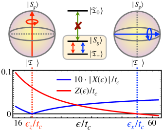
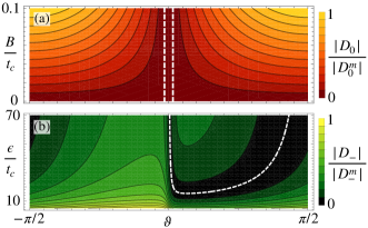
After introducing the model in Sec. II, we explicitly determine the optimal working points and derive effective singlet-triplet qubit Hamiltonians in Sec. III. When the system is operated at an optimal point, we find , where the ground state singlet and the triplet are the logical qubit states. The quantities and can be switched on and off by the adjusting the double-dot energy detuning (Fig. 1), hence offering all-electrical two-axes control over the qubit at a low leakage point. Since the axes are orthogonal, any one-qubit gate can be realized using three rotations [34], avoiding the more complicated control sequences required for non-orthogonal axes [35]. We proceed to consider the case of a strong SOI in Sec. IV and find that many of the desirable properties described in Sec. III still hold in this case. Finally, Sec. V provides a conclusion.
II Model Hamiltonian
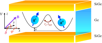
We consider a tunnel-coupled DQD with single particle tunneling matrix element in a regime where the (0,2) singlet is far detuned. A typcial architecture realizing the system as a planar DQD in a Ge-GeSi heterostructure is shown in Fig. 2. Allowing for spin-flip tunneling processes induced by the SOI and an external magnetic field of arbitrary direction, the Hamiltonian reads [36, 37],
| (1) | ||||
where is the detuning relative to the (1,1)-(2,0) singlet crossing, and is the spin-orbit vector of the system. Note that is scaled by a factor compared to Ref. [37] to unburden the notation and lighten the expressions later on. Information about the spin-orbit vector may be obtained, e.g., via magneto-transport measurements [38, 39]. Higher order contributions due to the SOI are possible but suppressed when the orbital spacing induced by the confinement potentials is the largest energy scale in the system [40]. Finally, the Zeeman Hamiltonian contains anisotropic site-dependent tensors which lead to additional coupling terms between singlets and triplets. In general, our analysis applies whenever the two tensors are diagonal in a common eigenbasis. In the following we take the tensor in each dot to be diagonal in the basis defined by the cubic crystal and degenerate in the --plane, . In all the plots in this paper, the tensor components are taken to have values typical for HHs in Ge, , , and , where labels the left/right dot. Parametrizing the magnetic field in spherical coordinates with the --plane as the equatorial plane and the azimuthal angle measured from the DQD axis , , the Zeeman Hamiltonian has the form
| (2) | ||||
where and are the sums and differences of the tensor components in the left and right dot.
The proposed model is rather general and may in principle be applied to a wide range of materials. However, the presence of site-dependent and highly anisotropic tensors in combination with a strong SOI is typical for HH states, e.g., in the semiconductor Ge. Moreover, the specialization of HH systems allows us to neglect interactions of the hole spins with the nuclear spin bath.
II.1 Dominant basis
Although the SOI and the site-dependence of the tensors are non negligible effects in HH systems, the largest energy scale is still expected to be given by the spin conserving tunnel coupling and the standard Zeeman terms featuring the sum of factors in the dots. The case where the spin-flip tunneling terms induced by the SOI are of the same order of magnitude as is discussed in Sec. IV. For now we work in the regime where the dominant part of the Hamiltonian is as given in Eq. (1) but for vanishing SOI () and equal tensors (). It is diagonal in the states,
| (3) | ||||
where we introduce the orbital hybridization angle for the hybridized singlets and the dimensionless functions , with the effective sum of factors,
| (4) |
for the mixed triplet states. Transforming into the basis yields a Hamiltonian in which the ground state singlet is separated from the triplets by the exchange energy , and which features the relevant singlet triplet mixing terms,
| (5) |
where for upper indices . The matrix elements due to the SOI are given by
| (6) | ||||
and the Hermiticity of the Hamiltonian is warranted by , while the effective two-particle factors read
| (7) | ||||
The term arises due to the anisotropy of the tensors and is only present when the magnetic field has non-zero in- and out-of-plane components, , i.e., when the field is not aligned with one of the principal axes of the tensor. Put differently, the term is a consequence of non-parallel effective magnetic fields in the dots , which enclose an angle
| (8) |
with the equatorial plane. Due to the inverse effect of increased HH light hole (LH) mixing on the tensor components, i.e., a reduction of the out-of-plane factor and an enhancement of the in-plane factor, one expects for and vice versa. Hence, the anisotropy term can be quite sizeable when the tensors are different. For isotropic tensors one has , and .
It is worth pointing out that the energies of the dominant eigenstates and the couplings between these states obtained by diagonalization of the dominant part of the Hamiltonian and the transformation of the non-dominant part into this basis agree with those obtained by naively choosing the global quantization axis along the sum of effective magnetic fields as detailed in Appendix A. This result is non-trivial as the quantization axis is fixed to be out-of-plane in two dimensional holes systems as a direct consequence of the spin-momentum locking in the Luttinger-Kohn Hamiltonian and the position-momentum uncertainty relation [30].
II.2 Symmetries of the system
The system possesses two symmetries which are not obvious from the Hamiltonian (II.1): time-reversal symmetry in combination with the inversion of the magnetic field and symmetry under the exchange of the two dots.
Firstly we note that under the combined inversion of time, , and the magnetic field, (i.e., ), one has and . Since furthermore and , the total Hamiltonian (II.1) is invariant, in particular for , where it is time-reversal invariant.
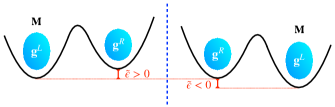
Secondly, we point out a symmetry under the exchange of the two dots. There is a peculiarity arising due to site-dependent anisotropic tensors. When exchanging the tensors, , one finds and which amounts to a relative minus in the coupling terms between the singlets and the triplets. As a consequence, the different tensors distinguish the left and right dot in a way that can be measured. To understand this observation, one must work in the enlarged six-dimensional Hilbert space, now containing both singlets with double dot occupancy, and , with energies and , respectively, being the charging energy and the energy detuning between the dots in the one particle picture. Note that the spin conserving tunnel matrix element has the same sign for tunneling events from to both and , while the spin-orbit matrix elements satisfy for . Consequently, the Hamiltonian is invariant with respect to exchanging the tensors if we furthermore invert the inter-dot detuning and relabel the states 111In addition, one must rescale the triplet states by minus one. However, since the physical states are only representatives of an entire ray of states in a Hilbert space, this minus only amounts to an irrelevant phase.. The combination of these transformations amounts to a complete reversal of the system architecture (Fig. 3). Experimentally, the change of the effective two-particle factors when exchanging the one-particle tensors reflects the fact that one arbitrarily chooses one site as the (doubly occupied) measurement point by choosing the sign of the inter dot detuning, e.g., for in this work.
III The spin-orbit switch
A spin-orbit switch is present in a system if the SOI can be turned on and off by changing external control parameters such as gate voltages or an applied magnetic field. When operating such a system one may utilize the SOI for one application, e.g., for spin qubit manipulation in the context of spintronics, while one may choose to turn it off for another, e.g., for the purpose of spin readout or for assessing the effect of (residual) nuclear spins in the system. Therefore, a spin-orbit switch is a highly desirable property in platforms used for quantum information processing. Recently, this functionality was reported for holes in a Ge/silicon core/shell nanowire [42].
The logical singlet-triplet qubit space is spanned by the ground state singlet and one of the hybridized triplet states . Hence, the relevant couplings are
| (9) |
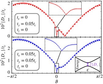
In our approach the mixing terms are obtained by an exact basis transformation, and there has been no approximation made so far. Whether the actual physical system is accurately described by the expressions (9) depends on the validity of the choice of basis, the requirement being that the diagonal terms in the Hamiltonian matrix (II.1) dominate over the off-diagonal terms. In Fig. 4 we compare the analytical expression for to the exact result obtained by numerical diagonalization of the Hamiltonian (1). We find excellent agreement, justifying our choice of basis even for relatively large out-of-plane factor differences () and spin-flip tunneling terms (). When the SOI becomes even larger, a different choice of basis can be more appropriate (Sec. IV). Note that when a Schrieffer-Wolff transformation is performed to decouple the excited singlet from the four dimensional low-energy space, the couplings are unchanged to leading order in the small quantities , , where is the energy separation between the low-lying states and , and , are the mixing terms. Finally, we note that couplings of the form (9) may be picked up experimentally by measuring the singlet return probability in combination with Landau-Zener schemes [43]. Since all four low-energy states interact, it can be necessary to perform an additional Schrieffer-Wolff transformation to obtain an effective two-level system for which the standard Landau-Zener formalism can be applied.
As can be seen from Eq. (II.1), there are two contributions to as defined in Eq. (9): the SOI via the terms ( and site-dependent tensors via () for (). As we will see, these terms may counteract for certain magnetic field angles and detunings such that , which effectively corresponds to a switched off SOI.
III.1 Longitudinal coupling
We first consider the coupling between the ground state singlet and the unpolarized (longitudinal) triplet . Introducing the sums and differences of effective magnetic fields for diagonal tensors in both dots, , we may write
| (10) | ||||
where with is the normalized version of and
| (11) |
Note that the scalar product in Eq. (10) is defined such that complex conjugation is performed in the first entry, . Since the spin-orbit vector is real, the vector is non-zero for non-vanishing and , and we have only when the vectors and are orthogonal.
A necessary condition for is and hence
| (12) |
Note that we expect as the out-of-plane factor decreases with stronger HH-LH mixing, while the in-plane factor increases. Hence, the radicand is positive and a real solution to Eq. (12) exists. One then finds the additional conditions for the azimuthal angle,
| (13) | ||||
Hence, the line of zero coupling is independent of the magnetic field strength and the detuning. A plot of the coupling for the case is shown in Fig. 5(a).
III.2 Transverse coupling
We now turn to the couplings between the ground state singlet and the polarized (transverse) triplets . A classification of magnetic degeneracy points in systems with site-dependent tensors and SOI was reported in Ref. [44]. At these degeneracy points the ground state becomes degenerate in energy, corresponding to a vanishing coupling between the two lowest lying states, in our case. In this section, we investigate how such points can be controlled by the model parameters, and additionally investigate the zeros of the other transverse coupling . Using the quantities introduced in Eqs. (10) and (11), one has
| (14) | ||||
where . In contrast to the scalar product, the cross product is defined without complex conjugation, with the totally anti-symmetric tensor . Zero coupling is achieved for
| (15) |
where corresponds to and the polar angle is expressed in terms of the azimuthal angle,
| (16) |
For a given spin-orbit vector Eq. (15) can be used to determine the values of , and for which the coupling vanishes. By substituting back into Eq. (16) one obtains the corresponding polar angle .
It is instructive to look at some special cases for the spin-orbit vector. If , one has by Eq. (16) and hence Eq. (15) is satisfied independently of , and . On the other hand, if , there are two configurations that lead to zero coupling: (i) If Eq. (16) is satisfied by setting , Eq. (15) requires since at finite detuning. (ii) Eq. (16) may also be satisfied by setting , remarkably the same azimuthal angle as required by Eq. (LABEL:eq:zero_line_d0_phi) for the longitudinal coupling to vanish. Eq. (15) then yields
| (17) |
where . The purely in-plane form of the spin-orbit vector is of particular interest as it is predicted, e.g., for HHs in planar Ge due to the cubic Rashba SOI [9] and for holes in Ge/Si nanowires [42]. Note that in contrast to the longitudinal case discussed above, the spin-orbit switch can be operated electrically via the parameter , suggesting the possibility of fast and accurate control over the SOI. We display the form of the coupling for exemplary values in Fig. 5(b).
On the grounds of symmetry considerations, it is in principle possible that the in-plane degeneracy of the tensor in HH systems can be lifted if the confinement potential in the dots is elliptical. The broken in-plane symmetry allows for HH-LH induced corrections to the factors yielding . However, this will leave the above results unchanged if the magnetic field is applied along one of the principal axes of the elliptical confinement potential, or .
Finally, we point out another application of our results, which is the reverse argumentation of before. By studying the avoided crossing between the ground state singlet and one of the triplet states, one may obtain information about the SOI in the system if the tensors are known, e.g., from magneto-transport measurements [45, 46]. The experimental parameters used when the crossing vanishes, e.g. the detuning and magnetic field settings, allow for a determination of the spin-orbit vector. If the tensors and the spin-orbit vector are known, one may estimate the effect of the nuclear spin bath. Similar schemes have been proposed for systems with equal and isotropic tensors but non-negligible hyperfine interactions [47] and in-plane magnetic fields [48].
III.3 Effective qubit Hamiltonians
Having analyzed the form of the longitudinal and transverse coupling terms, we proceed to study two possible qubit realizations that can benefit from the dependence of the couplings on the magnetic field direction and the detuning described above. First, we consider a - qubit, i.e., a qubit defined by the ground state singlet and the unpolarized mixed triplet . By projecting the total Hamiltonian (II.1) onto the logical basis, we find the effective qubit Hamiltonian
| (18) |
Since the logical subspace is not ideally decoupled, corrections due to mixing with states outside the qubit space arise. Computing these corrections by means of a Schrieffer-Wolff transformation, however, we find that they are negligible as long as (Appendix B). Moreover, the quality of the approximation increases and leakage errors can be avoided by fixing the magnetic field direction such that [cf. Eqs. (15) and (16)]. The coupling can then be switched on and off via electrical factor engineering [49, 50, 51] [cf. Eq. (12)] or by controlling the spin-flip tunneling elements [cf. Eq. (LABEL:eq:zero_line_d0_phi)] which are expected to depend on the gate voltages through the applied potential [9].
More direct control via the detuning is possible by defining the qubit via the two lowest lying states and . For the qubit subspace is well isolated (cf. Fig. 4) and by again projecting the total Hamiltonian (II.1) onto the logical basis, we obtain the effective qubit Hamiltonian
| (19) |
up to an irrelevant total shift in energy. For a realistic form of the SOI with as discussed above, one may set by fixing the magnetic field such that and takes the value specified in Eq. (12), resulting in a strong suppression of leakage errors (see Appendix B and Fig. 7(c) therein). By Eq. (17), one then has control over the coupling , which is a purely real quantity at the optimal value of , by varying the detuning , in particular the coupling can be switched on and off electrically. This supplies us with an electrically tunable two-axes control over the qubit. When the detuning is chosen such that (), the Hamiltonian generates -rotations (-rotations), and the specific values for () can be obtained from Eq. (II.1) and Eq. (17), respectively,
| (20) | ||||
| (21) |
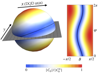
We display the dependence of the elements in the - qubit Hamiltonian (19) on the detuning in a region including and in Fig. 1. In the same figure we show the Bloch sphere corresponding to the effective two-level system and the orthogonal rotation axes obtained for the two different values of the detuning. We fix the magnetic field at an optimal point by choosing and such that [cf. Eqs. (12) and (LABEL:eq:zero_line_d0_phi)], identify and , and set and . Note that even at the relatively low magnetic field mT leakage to the only relevant coupled state is negligible (Appendix B). At this point, one has and , allowing for Rabi -rotations in the GHz range and -rotations at tens of MHz. Hence, it is feasible to operate the system below the critical field of conventional superconductors such as aluminum, suggesting that all-electrically controllable, fast - qubits can be coupled using superconducting transmission lines [52, 53].
IV Strong spin-orbit interaction
For systems where the elements of the spin-orbit vector are comparable in magnitude to the tunnel coupling , the states defined in Eq. (3) will no longer provide an appropriate basis. Moreover, since low magnetic fields are attractive considering integration of the qubit with superconducting resonators, it is natural to study the regime . One may then exactly diagonalize the dominant part of the Hamiltonian and treat the Zeeman term as a small perturbation. We find three degenerate states , , mixing all (1,1) states with zero energy and two states that also contain an admixture of the (2,0) singlet with energies
| (22) |
The exact form of the eigenstates can be found in Appendix C. We may identify the states and in the sense that they will transition into each other for . At zero magnetic field the states with form an eigenspace with zero energy. Looking at their behaviour at finite field as tends to zero we may identify . Hence, if we are interested in singlet-triplet like mixing, the relevant couplings are induced by the Zeeman term,
| (23) |
where and the functions contain all information about anisotropic site-dependent tensors and the SOI. As a consequence, the non-trivial zeros of are determined by the orientation of the magnetic field alone. We note that as in Sec. III the expressions are unchanged when we decouple the energetically high lying state via a Schrieffer-Wolff transformation to leading order in where the denominator denotes the energy separation between the states in the subspaces and is the relevant scale of the mixing terms.
Clearly, in an eigenbasis of , the SOI does not amount to a coupling of the eigenstates. One may then control the couplings simply by tuning the magnitude of the magnetic field. However, for gate operation it is desirable to have the coupling between the logical qubit states (e.g., turned on), while all other couplings should be absent to avoid leakage errors. This can be achieved by controlling the orientation of the magnetic field relative to the spin-orbit vector. The explicit form of the couplings is easily computed from Eq. (23) but lengthy, and we restrict our attention to determining the the points where .
One finds for any azimuthal angle as long as the polar angle is chosen such that
| (24) | ||||
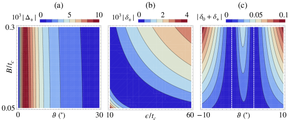
We display the absolute value of and its dependence on the magnetic field direction for exemplary values of the spin-orbit vector in Fig. 6. Moreover, we find if the following conditions are satisfied,
| (25) | ||||
and for
| (26) | ||||
For a given spin-orbit vector, the conditions (LABEL:eq:C0_zero)-(26) can easily be rearranged to obtain the angles and solely in terms of the tunnel coupling, the spin-orbit vector and the factors.
Finally, we consider the special case of an in-plane spin-orbit vector as in Sec. III. We encode the qubit in the states and , which are split by the modified exchange energy,
| (27) |
at zero magnetic field. As can be seen from Eqs. (25) and (26), we may set by choosing
| (28) |
For these values, one has and so the qubit ground state is completely decoupled from the states outside the logical subspace but coupled to the excited qubit state; the strength of the coupling can be controlled by the magnitude of the magnetic field . Of course, the coupling cannot be made arbitrarily large in this way since the condition must be met to ensure that the approach presented in this section can accurately describe the physical system.
V Conclusion
Starting from a general phenomenological model for spins confined in a DQD system subject to a magnetic field, we show the existence of magnetic field strengths and directions where the coupling between the ground state singlet and the triplet states vanishes. The effect is due to cancelling contributions from the SOI and anisotropic site-dependent tensors, both of which are characteristic features of semiconductor hole systems. With the magnetic field fixed at one such optimal point one may avoid leakage to states outside the logical subspace and at the same time operate the qubit all-electrically. In particular, we demonstrate that for realistic system parameters an electric spin-orbit switch can be implemented and controlled by the detuning, allowing for highly tunable two-axes control in hole singlet-triplet qubits. This property can be used in quantum information processing units built from singlet-triplet qubits to tune into regimes best suited for the tasks of readout and initialization (low coupling) as well as qubit manipulation (high coupling). Since fast operations at optimal points are feasible at low magnetic fields ( mT), different singlet-triplet qubits can be interconnected using superconducting resonators.
Moreover, we study systems with a strong SOI operated at low magnetic fields, and demonstrate that for a realistic form of the spin-orbit vector there exists a particular direction of the magnetic field where the coupling between the qubit ground state and states outside the logical subspace can be set to zero. At this optimal point the qubit ground state is protected from leakage errors, and the strength of the coupling to the excited qubit state can be tuned by the magnitude of the magnetic field.
Future research may focus on the precise form of the SOI, e.g., in two-dimensional Ge HH systems to include effects such as a magnetic field dependence of the spin-orbit elements as well as spin-orbit terms induced by magnetic fields which are not time reversal invariant and thus not described by the model used in this work.
VI Acknowledgements
We would like to thank Daniel Jirovec and Georgios Katsaros for insightful discussions on hole systems in planar germanium. This research is supported by the German Research Foundation (Deutsche Forschungsgemeinschaft, DFG) under project number 450396347.
Appendix A Fixing the quantization axis
In this appendix we relate the results of the main text to the case where one may choose the orientation of the quantization axis freely. Defining the spin operators and the effective magnetic field in dot as and , respectively, one finds for the Zeeman Hamiltonian,
| (29) | ||||
where we define . Choosing the quantization axis along and denoting this direction by , we find by decomposing into components parallel and perpendicular to ,
| (30) | ||||
where the effective factors are as given in Eq. (7) and is the spin operator along , . The angle only amounts to an irrelevant phase and may thus be set to zero. One can see from the Hamiltonian (30) that the hybridized triplets (3) are the same as those obtained by choosing the quantization axis along the sum of effective magnetic fields.
While the form of the part of the Hamiltonian describing the detuning and tunneling between the singlets is invariant under a change of the quantization axis, the part of the Hamiltonian describing the SOI may be transformed into the basis defined by the above choice of the quantization axis, and we recover the matrix elements in Eq. (6) after performing an additional transformation into the basis of hybridized singlets [cf. Eq. (3)].
Appendix B Effective qubit Hamiltonians and leakage
In this appendix we quantify our claim of Sec. III and show that the effective qubit Hamiltonians shown in Eqs. (18) and (19) are accurate since leakage to states outside the logical subspace is suppressed. For this purpose we decouple the qubit space from the remaining states in the (1,1) charge configuration by means of a Schrieffer-Wolff transformation.
For the Hamiltonian in Eq. (18), the logical subspace is spanned by the states and . Upon application of a Schrieffer-Wolff transformation, these states will be changed to the perturbed states and , and we find to leading order,
| (31) | ||||
where
| (32) |
At we recover Eq. (18) of the main text. Working at an optimal point, we can achieve by fixing the direction of the magnetic field or the detuning according to Eqs. (15) and (16). The term then determines the remaining leakage out of the original logical subspace , to the state .
An analogous analysis applies for the case of the - qubit Hamiltonian (19), yielding
| (33) | ||||
where
| (34) | |||
| (35) |
One may achieve by choosing the magnetic field orientation according to Eqs. (12) and (LABEL:eq:zero_line_d0_phi). At this point the term determines the residual leakage out of the original logical subspace , to the state .
As can be seen from Fig. 7, the leakage for both qubits discussed above is well below one percent for realistic parameter settings. For the - qubit, the detuning can be chosen such that . On the other hand, for the - qubit, one has at for the detuning values required for gate operation (cf. Fig. 1). Fig. 7(c) highlights the strong suppression of leakage in the - qubit at an optimal point with , emphasizing the importance of operating the singlet-triplet qubit at the optimal points reported in this paper.
Appendix C Eigenbasis of the orbital and spin-orbit Hamiltonian
The Hamiltonian given in Eq. (1) of the main text may be diagonalized exactly, yielding the orthonormal eigenstates,
| (36) | ||||
| (37) | ||||
| (38) | ||||
| (39) |
where . The states , , are degenerate with zero energy and have been orthogonalized by hand, while the states have energies
| (40) |
References
- Hendrickx et al. [2020a] N. Hendrickx, D. Franke, A. Sammak, G. Scappucci, and M. Veldhorst, Fast two-qubit logic with holes in germanium, Nature 577, 487 (2020a).
- Hendrickx et al. [2020b] N. Hendrickx, W. Lawrie, L. Petit, A. Sammak, G. Scappucci, and M. Veldhorst, A single-hole spin qubit, Nat. Commun. 11, 3478 (2020b).
- Wang et al. [2020] K. Wang, G. Xu, F. Gao, H. Liu, R.-L. Ma, X. Zhang, T. Zhang, G. Cao, T. Wang, J.-J. Zhang, X. Hu, H.-W. Jiang, H.-O. Li, G.-C. Guo, and G.-P. Guo, Ultrafast operations of a hole spin qubit in Ge quantum dot (2020), arXiv:2006.12340 [cond-mat.mes-hall] .
- Lawrie et al. [2020] W. I. L. Lawrie, N. W. Hendrickx, F. van Riggelen, M. Russ, L. Petit, A. Sammak, G. Scappucci, and M. Veldhorst, Spin relaxation benchmarks and individual qubit addressability for holes in quantum dots, Nano Letters 20, 7237 (2020).
- van Riggelen et al. [2021] F. van Riggelen, N. W. Hendrickx, W. I. L. Lawrie, M. Russ, A. Sammak, G. Scappucci, and M. Veldhorst, A two-dimensional array of single-hole quantum dots, Applied Physics Letters 118, 044002 (2021).
- Hendrickx et al. [2021] N. W. Hendrickx, W. I. Lawrie, M. Russ, F. van Riggelen, S. L. de Snoo, R. N. Schouten, A. Sammak, G. Scappucci, and M. Veldhorst, A four-qubit germanium quantum processor, Nature 591, 580 (2021).
- Wang et al. [2021] Z. Wang, E. Marcellina, A. Hamilton, J. H. Cullen, S. Rogge, J. Salfi, and D. Culcer, Optimal operation points for ultrafast, highly coherent Ge hole spin-orbit qubits, npj Quantum Inf 7, 54 (2021).
- Mutter and Burkard [2020a] P. M. Mutter and G. Burkard, Cavity control over heavy-hole spin qubits in inversion-symmetric crystals, Phys. Rev. B 102, 205412 (2020a).
- Mutter and Burkard [2021a] P. M. Mutter and G. Burkard, Natural heavy-hole flopping mode qubit in germanium, Phys. Rev. Research 3, 013194 (2021a).
- Benito et al. [2017] M. Benito, X. Mi, J. M. Taylor, J. R. Petta, and G. Burkard, Input-output theory for spin-photon coupling in Si double quantum dots, Phys. Rev. B 96, 235434 (2017).
- Mi et al. [2018] X. Mi, M. Benito, S. Putz, D. M. Zajac, J. M. Taylor, G. Burkard, and J. R. Petta, A coherent spin-photon interface in silicon, Nature 555, 599 (2018).
- Benito et al. [2019a] M. Benito, J. R. Petta, and G. Burkard, Optimized cavity-mediated dispersive two-qubit gates between spin qubits, Phys. Rev. B 100, 081412 (2019a).
- Benito et al. [2019b] M. Benito, X. Croot, C. Adelsberger, S. Putz, X. Mi, J. R. Petta, and G. Burkard, Electric-field control and noise protection of the flopping-mode spin qubit, Phys. Rev. B 100, 125430 (2019b).
- Croot et al. [2020] X. Croot, X. Mi, S. Putz, M. Benito, F. Borjans, G. Burkard, and J. R. Petta, Flopping-mode electric dipole spin resonance, Phys. Rev. Research 2, 012006 (2020).
- Levy [2002] J. Levy, Universal quantum computation with spin- pairs and heisenberg exchange, Phys. Rev. Lett. 89, 147902 (2002).
- Petta et al. [2005] J. R. Petta, A. C. Johnson, J. M. Taylor, E. A. Laird, A. Yacoby, M. D. Lukin, C. M. Marcus, M. P. Hanson, and A. C. Gossard, Coherent manipulation of coupled electron spins in semiconductor quantum dots, Science 309, 2180 (2005).
- Foletti et al. [2009] S. Foletti, H. Bluhm, D. Mahalu, V. Umansky, and A. Yacoby, Universal quantum control of two-electron spin quantum bits using dynamic nuclear polarization, Nature Phys 5, 903 (2009).
- Wu et al. [2014] X. Wu, D. R. Ward, J. R. Prance, D. Kim, J. K. Gamble, R. T. Mohr, Z. Shi, D. E. Savage, M. G. Lagally, M. Friesen, S. N. Coppersmith, and M. A. Eriksson, Two-axis control of a singlet–triplet qubit with an integrated micromagnet, Proceedings of the National Academy of Sciences 111, 11938 (2014).
- Nichol et al. [2017] J. M. Nichol, L. A. Orona, S. P. Harvey, S. Fallahi, G. C. Gardner, M. J. Manfra, and A. Yacoby, High-fidelity entangling gate for double-quantum-dot spin qubits, npj Quantum Inf 3, 3 (2017).
- Koppens et al. [2005] F. H. L. Koppens, J. A. Folk, J. M. Elzerman, R. Hanson, L. H. W. van Beveren, I. T. Vink, H. P. Tranitz, W. Wegscheider, L. P. Kouwenhoven, and L. M. K. Vandersypen, Control and detection of singlet-triplet mixing in a random nuclear field, Science 309, 1346 (2005).
- Maune et al. [2014] B. M. Maune, M. G. Borselli, B. Huang, T. D. Ladd, P. W. Deelman, K. S. Holabird, A. A. Kiselev, I. Alvarado-Rodriguez, R. S. Ross, A. E. Schmitz, M. Sokolich, C. A. Watson, M. F. Gyure, and A. T. Hunter, Coherent singlet-triplet oscillations in a silicon-based double quantum dot, Nature 481, 344 (2014).
- Jock et al. [2018] R. M. Jock, N. T. Jacobson, P. Harvey-Collard, A. M. Mounce, V. Srinivasa, D. R. Ward, J. Anderson, R. Manginell, J. R. Wendt, M. Rudolph, T. Pluym, J. K. Gamble, A. D. Baczewski, W. M. Witzel, and M. S. Carroll, A silicon metal-oxide-semiconductor electron spin-orbit qubit, Nat Commun 9, 1768 (2018).
- [23] A. Hofmann, D. Jirovec, M. Borovkov, I. Prieto, A. Ballabio, J. Frigerio, D. Chrastina, G. Isella, and G. Katsaros, arXiv:1910.05841 [cond-mat.mes-hall] .
- Jirovec et al. [2021] D. Jirovec, A. Hofmann, A. Ballabio, P. M. Mutter, G. Tavani, M. Botifoll, A. Crippa, J. Kukucka, O. Sagi, F. Martins, J. Saez-Mollejo, I. Prieto, M. Borovkov, J. Arbiol, D. Chrastina, G. Isella, and G. Katsaros, A singlet-triplet hole spin qubit in planar Ge, Nature Materials (2021).
- Burkard et al. [2020] G. Burkard, M. J. Gullans, X. Mi, and J. Petta, Superconductor–semiconductor hybrid-circuit quantum electrodynamics, Nat. Rev. Phys. 2, 129 (2020).
- Fischer et al. [2009] J. Fischer, M. Trif, W. A. Coish, and D. Loss, Spin interactions, relaxation and decoherence in quantum dots, Solid State Communications 149, 1443 (2009).
- Fischer and Loss [2010] J. Fischer and D. Loss, Hybridization and spin decoherence in heavy-hole quantum dots, Phys. Rev. Lett. 105, 266603 (2010).
- Maier and Loss [2012] F. Maier and D. Loss, Effect of strain on hyperfine-induced hole-spin decoherence in quantum dots, Phys. Rev. B 85, 195323 (2012).
- Sigillito et al. [2015] A. J. Sigillito, R. M. Jock, A. M. Tyryshkin, J. W. Beeman, E. E. Haller, K. M. Itoh, and S. A. Lyon, Electron spin coherence of shallow donors in natural and isotopically enriched germanium, Phys. Rev. Lett. 115, 247601 (2015).
- Scappucci et al. [2020] G. Scappucci, C. Kloeffel, F. A. Zwanenburg, D. Loss, M. Myronov, J.-J. Zhang, S. D. Franceschi, G. Katsaros, and M. Veldhorst, The germanium quantum information route, Nat. Rev. Mater. (2020).
- Bulaev and Loss [2005a] D. V. Bulaev and D. Loss, Spin relaxation and decoherence of holes in quantum dots, Phys. Rev. Lett. 95, 076805 (2005a).
- Bulaev and Loss [2005b] D. V. Bulaev and D. Loss, Spin relaxation and anticrossing in quantum dots: Rashba versus dresselhaus spin-orbit coupling, Phys. Rev. B 71, 205324 (2005b).
- Bulaev and Loss [2007] D. V. Bulaev and D. Loss, Electric dipole spin resonance for heavy holes in quantum dots, Phys. Rev. Lett. 98, 097202 (2007).
- Barenco et al. [1995] A. Barenco, C. H. Bennett, R. Cleve, D. P. DiVincenzo, N. Margolus, P. Shor, T. Sleator, J. A. Smolin, and H. Weinfurter, Elementary gates for quantum computation, Phys. Rev. A 52, 3457 (1995).
- Hanson and Burkard [2007] R. Hanson and G. Burkard, Universal set of quantum gates for double-dot spin qubits with fixed interdot coupling, Phys. Rev. Lett. 98, 050502 (2007).
- Jouravlev and Nazarov [2006] O. N. Jouravlev and Y. V. Nazarov, Electron transport in a double quantum dot governed by a nuclear magnetic field, Phys. Rev. Lett. 96, 176804 (2006).
- Danon and Nazarov [2009] J. Danon and Y. V. Nazarov, Pauli spin blockade in the presence of strong spin-orbit coupling, Phys. Rev. B 80, 041301 (2009).
- Mutter and Burkard [2020b] P. M. Mutter and G. Burkard, g-tensor resonance in double quantum dots with site-dependent g-tensors, Mater. Quantum. Technol. 1, 015003 (2020b).
- Mutter and Burkard [2021b] P. M. Mutter and G. Burkard, Pauli spin blockade with site-dependent tensors and spin-polarized leads, Phys. Rev. B 103, 245412 (2021b).
- Golovach et al. [2004] V. N. Golovach, A. Khaetskii, and D. Loss, Phonon-induced decay of the electron spin in quantum dots, Phys. Rev. Lett. 93, 016601 (2004).
- Note [1] In addition, one must rescale the triplet states by minus one. However, since the physical states are only representatives of an entire ray of states in a Hilbert space, this minus only amounts to an irrelevant phase.
- Froning et al. [2021a] F. N. M. Froning, L. C. Camenzind, O. A. H. van der Molen, A. Li, E. P. A. M. Bakkers, D. M. Zumbühl, and F. R. Braakman, Ultrafast hole spin qubit with gate-tunable spin-orbit switch, Nat. Nanotechnol. 16, 308 (2021a).
- Petta et al. [2010] J. R. Petta, H. Lu, and A. C. Gossard, A coherent beam splitter for electronic spin states, Science 327, 669 (2010).
- Frank et al. [2020] G. Frank, Z. Scherübl, S. Csonka, G. Zaránd, and A. Pályi, Magnetic degeneracy points in interacting two-spin systems: Geometrical patterns, topological charge distributions, and their stability, Phys. Rev. B 101, 245409 (2020).
- Froning et al. [2021b] F. N. M. Froning, M. J. Rančić, B. Hetényi, S. Bosco, M. K. Rehmann, A. Li, E. P. A. M. Bakkers, F. A. Zwanenburg, D. Loss, D. M. Zumbühl, and F. R. Braakman, Strong spin-orbit interaction and -factor renormalization of hole spins in Ge/Si nanowire quantum dots, Phys. Rev. Research 3, 013081 (2021b).
- Zhang et al. [2021] T. Zhang, H. Liu, F. Gao, G. Xu, K. Wang, X. Zhang, G. Cao, T. Wang, J. Zhang, X. Hu, and et al., Anisotropic g-factor and spin–orbit field in a germanium hut wire double quantum dot, Nano Letters 21, 3835–3842 (2021).
- Stepanenko et al. [2012] D. Stepanenko, M. Rudner, B. I. Halperin, and D. Loss, Singlet-triplet splitting in double quantum dots due to spin-orbit and hyperfine interactions, Phys. Rev. B 85, 075416 (2012).
- Nowak et al. [2011] M. P. Nowak, B. Szafran, F. M. Peeters, B. Partoens, and W. J. Pasek, Tuning of the spin-orbit interaction in a quantum dot by an in-plane magnetic field, Phys. Rev. B 83, 245324 (2011).
- Nakaoka et al. [2007] T. Nakaoka, S. Tarucha, and Y. Arakawa, Electrical tuning of the factor of single self-assembled quantum dots, Phys. Rev. B 76, 041301 (2007).
- Prechtel et al. [2015] J. H. Prechtel, F. Maier, J. Houel, A. V. Kuhlmann, A. Ludwig, A. D. Wieck, D. Loss, and R. J. Warburton, Electrically tunable hole factor of an optically active quantum dot for fast spin rotations, Phys. Rev. B 91, 165304 (2015).
- Voisin et al. [2016] B. Voisin, R. Maurand, S. Barraud, M. Vinet, X. Jehl, M. Sanquer, J. Renard, and S. De Franceschi, Electrical control of g-factor in a few-hole silicon nanowire mosfet, Nano Letters 16, 88 (2016).
- Burkard and Imamoglu [2006] G. Burkard and A. Imamoglu, Ultra-long-distance interaction between spin qubits, Phys. Rev. B 74, 041307 (2006).
- Jin et al. [2012] P.-Q. Jin, M. Marthaler, A. Shnirman, and G. Schön, Strong coupling of spin qubits to a transmission line resonator, Phys. Rev. Lett. 108, 190506 (2012).