Heating Rates under Fast Periodic Driving beyond Linear Response

Abstract

Heating under periodic driving is a generic nonequilibrium phenomenon, and it is a challenging problem in nonequilibrium statistical physics to derive a quantitatively accurate heating rate. In this work, we provide a simple formula on the heating rate under fast and strong periodic driving in classical and quantum many-body systems. The key idea behind the formula is constructing a time-dependent dressed Hamiltonian by moving to a rotating frame, which is found by a truncation of the high-frequency expansion of the micromotion operator, and applying the linear-response theory. It is confirmed for specific classical and quantum models that the second-order truncation of the high-frequency expansion yields quantitatively accurate heating rates beyond the linear-response regime. Our result implies that the information on heating dynamics is encoded in the first few terms of the high-frequency expansion, although heating is often associated with an asymptotically divergent behavior of the high-frequency expansion.

Introduction.— Fast periodic driving in thermally isolated many-body systems can stabilize interesting many-body states. Theoretically, by using the high-frequency expansion of the Floquet operator, we can obtain a static effective Hamiltonian that describes the property of such a stabilized state, and interesting phases have been theoretically predicted Bukov et al. (2015); Eckardt (2017); Oka and Kitamura (2019). Recent experimental developments allow us to realize some of those nonequilibrium phases Zenesini et al. (2009); Aidelsburger et al. (2013); Miyake et al. (2013); Jotzu et al. (2014); Grushin et al. (2014); Meinert et al. (2016) and have triggered active research on the Floquet engineering (see Ref. Oka and Kitamura (2019) for a recent review).

Stability of such nonequilibrium phases is limited by heating due to periodic driving. It is therefore practically important to evaluate the heating rate. The rigorous approach has made significant progress in this field. It is rigorously proved that the heating is exponentially suppressed at high frequencies Abanin et al. (2015); Mori et al. (2016); Kuwahara et al. (2016); Abanin et al. (2017a, b). This phenomenon is known as the Floquet prethermalization Mori et al. (2018), which has also been experimentally observed Rubio-Abadal et al. (2020); Peng et al. (2021). However, the rigorous approach so far is limited to quantum systems with a bounded energy spectrum (i.e. quantum spin systems) and classical spin systems Mori (2018). Moreover, those rigorous results just give relatively loose upper bounds on the heating rate.

It is a theoretical challenge in nonequilibrium statistical physics to give a quantitatively accurate estimation of the heating rate for a wider class of many-body systems. For this purpose, the statistical approach is promising, in which the heating rate is evaluated by investigating the statistical probability of many-body resonances Rajak et al. (2018, 2019); Dalla Torre and Dentelski (2021). This approach is not rigorous, but instead, it gives approximate heating rates for generic systems including unbounded quantum and classical systems. Indeed, Floquet prethermalization in classical systems has been first established along this approach Rajak et al. (2018). The evaluation of the heating rate using Fermi’s golden rule for quantum systems Mallayya and Rigol (2019); Rakcheev and Läuchli and the energy diffusion theory for classical systems Hodson and Jarzynski (2021) can be categorized to this approach. However, such treatments have successfully given accurate heating rates only for weak driving. For modest or strong driving, which is needed for Floquet engineering, we need a new theoretical idea to achieve the goal.

In this Letter, we develop the statistical approach to the heating dynamics under strong driving, and obtain a simple analytical formula on the heating rate. The formula is obtained by finding a rotating frame in which driving looks weak enough. Such a rotating frame is found by using the technique of the high-frequency expansion  Bukov et al. (2015); Eckardt (2017); Mikami et al. (2016). The Hamiltonian in the rotating frame is called the dressed Hamiltonian, which is still time-periodic but has much weaker driving amplitude. Consequently, the linear response argument is valid for the dressed Hamiltonian rather than for the bare Hamiltonian, even when the original driving field is strong enough to being out of the linear response regime.

In a recent work Ikeda and Polkovnikov (2021), Fermi’s golden rule is extended to strong driving by utilizing the high-frequency expansion, which is conceptually close to the present work. However, our formulation importantly differs from the one in Ref. Ikeda and Polkovnikov (2021). The heating-rate formula obtained in Ref. Ikeda and Polkovnikov (2021) requires the exact Floquet operator (i.e. the time evolution operator over a cycle), which is not desirable feature. As a practical problem, this fact prevents us from applying the theory to classical systems, in which the Floquet operator is not accessible even numerically Mori (2018). On the other hand, the formula given in this Letter does not refer to the exact Floquet operator: the formula is completely written in terms of a truncated high-frequency expansion, which is accessible even for classical systems Mori (2018); Higashikawa et al. . This fact tells us that information on heating under fast and strong driving is encoded in the first few terms of the high-frequency expansion, which is an important theoretical observation not found in the previous studies.

In the following, we first describe how to get a dressed Hamiltonian via the high-frequency expansion. We then give linear response formulae on the heating rate in terms of the dressed Hamiltonian. Next, we numerically evaluate heating rates in specific classical and quantum spin systems and compare them with our theoretical predictions. Finally, we conclude our work with some remarks and future prospects.

Dressed Hamiltonian.— For notational simplicity, we first focus on quantum systems, and later discuss classical systems. Suppose a quantum system with a time-periodic Hamiltonian $H(t)=H_{0}+V(t)$ with $V(t)=\sum_{m=-\infty}^{\infty}V_{m}e^{-im\omega t}$ with $V_{0}=0$ and $V_{-m}=V_{m}^{\dagger}$ (in classical systems $\dagger$ should be interpreted as the complex conjugate), where the frequency is denoted by $\omega$ and the period is given by $T=2\pi/\omega$. The Floquet theorem states that the time evolution operator $U_{t,t_{0}}$ from time $t_{0}$ to $t$ is expressed as $U_{t,t_{0}}=e^{-iK(t)}e^{-iH_{F}(t-t_{0})/\hbar}e^{iK(t_{0})}$, where a time-periodic Hermitian operator $K(t)=K(t+T)$ is called the micromotion operator or the kick operator, and $H_{F}$ is called the Floquet Hamiltonian Bukov et al. (2015). It is noted that the choice of $K(t)$ and $H_{F}$ is not unique: Defining $e^{iK^{\prime}(t)}=U^{\dagger}e^{iK(t)}$ and $H_{F}^{\prime}=U^{\dagger}H_{F}U$ for any time-independent unitary operator $U$, we find $U_{t,t_{0}}=e^{-iK^{\prime}(t)}e^{-iH_{F}^{\prime}(t-t_{0})}e^{iK^{\prime}(t_{0})}$. In the high-frequency limit $\omega\to\infty$, $K(t)$ becomes constant, and hence we require $\lim_{\omega\to\infty}K(t)=0$ for convenience.

Since $U_{t,t_{0}}$ satisfies $i\hbar dU_{t,t_{0}}/dt=H(t)U_{t,t_{0}}$, the micromotion operator and the Floquet operator are related with each other via the equality

$$H_{F}=e^{iK(t)}\left[H(t)-i\hbar\frac{d}{dt}\right]e^{-iK(t)}.$$ (1)

This equation is interpreted as follows. Let us move to the “rotating frame” associated with the unitary transformation $e^{iK(t)}$. The Schrödinger equation $i\hbar d\ket{\psi(t)}/dt=H(t)\ket{\psi(t)}$ is transformed to

$$i\hbar\frac{d\ket{\psi^{\prime}(t)}}{dt}=H_{F}\ket{\psi^{\prime}(t)},$$ (2)

where $\ket{\psi^{\prime}(t)}=e^{iK(t)}\ket{\psi(t)}$ is the quantum state in the rotating frame. That is, the Hamiltonian in the rotating frame is given by $H_{F}$, and the time dependence of the Hamiltonian is completely removed.

Although $H_{F}$ contains full information on the long-time evolution including the heating rate, $H_{F}$ is highly nonlocal and quite complicated in many-body systems D’Alessio and Rigol (2014); Lazarides et al. (2014) and it is difficult to extract dynamical properties from $H_{F}$. It is also a hard task to numerically obtain $K(t)$ and $H_{F}$ exactly.

For fast driving, we can construct high-frequency expansions of $K(t)$ and $H_{F}$, which are accessible analytically and numerically. Because of the non-uniqueness of $K(t)$ and $H_{F}$, there are various high-frequency expansions Mikami et al. (2016). In this work, we focus on the van Vleck expansion Eckardt and Anisimovas (2015); Bukov et al. (2015) because of its analytical simplicity. The formulation given below is also applicable to other high-frequency expansions such as the Floquet-Magnus expansion Kuwahara et al. (2016); Mori et al. (2016).

The van Vleck high-frequency expansion is formally written in the following form:

$$K(t)=\sum_{k=1}^{\infty}\frac{\Lambda_{k}(t)}{\omega^{k}},\quad H_{F}=H_{0}+\sum_{k=1}^{\infty}\frac{\Omega_{k}}{\omega^{k}}.$$ (3)

The first two terms of the expansions are explicitly given by

$$i\hbar\Lambda_{1}(t)=-\sum_{m\neq 0}\frac{V_{m}}{m}e^{-im\omega t}, \Omega_{1}=\sum_{m\neq 0}\frac{[V_{-m},V_{m}]}{2m\hbar}$$ (4)

and

$$\left\{\begin{aligned} &i\hbar^{2}\Lambda_{2}(t)=\sum_{m\neq 0}\left(\frac{[V_{m},H_{0}]}{m^{2}}+\sum_{n\neq 0,m}\frac{[V_{n},V_{m-n}]}{mn}\right)e^{-im\omega t},\\ &\Omega_{2}=\sum_{m\neq 0}\left(\frac{[[V_{-m},H_{0}],V_{m}]}{2\hbar^{2}m^{2}}+\sum_{n\neq 0,m}\frac{[[V_{-m},V_{m-n}],V_{n}]}{3\hbar^{2}mn}\right).\end{aligned}\right.$$ (5)

Additional details on the van Vleck expansion as well as an explicit form of $\Lambda_{3}(t)$ are given in Supplementary Material (SM) SM (also see Ref. Mikami et al. (2016)).

It should be noted that this expansion is an asymptotic expansion in the thermodynamic limit Mori et al. (2016), and hence we should truncate the expansion to obtain a meaningful result. We define the $n$th order truncation of the expansion of $K(t)$ and $H_{F}$ as $K^{(n)}(t)=\sum_{k=1}^{n}\Lambda_{k}/\omega^{k}$ and $H_{F}^{(n)}=\sum_{k=0}^{n}\Omega_{k}/\omega^{k}$, respectively.

Let us move to the rotating frame associated with $K^{(n)}(t)$ rather than $K(t)$. The Hamiltonian in this rotating frame is given by

$$e^{-iK^{(n)}(t)}\left[H(t)-i\hbar\frac{d}{dt}\right]e^{iK^{(n)}t}\simeq\tilde{H}^{(n)}(t)$$ (6)

up to $O(\omega^{-n})$, where the $n$th order dressed Hamiltonian $\tilde{H}^{(n)}$ is given by

$$\tilde{H}^{(n)}(t)=H_{F}^{(n)}+V^{(n)}(t).$$ (7)

Its static part is nothing but the $n$th order truncation of the Floquet Hamiltonian. In SM SM, it is shown that the dressed driving $V^{(n)}(t)$ is expressed as

$$V^{(n)}(t)=\frac{\hbar}{\omega^{n+1}}\frac{d\Lambda_{n+1}(t)}{dt}.$$ (8)

We find that $V^{(n)}(t)$ satisfies the desirable property of periodic driving: $V^{(n)}(t)=V^{(n)}(t+T)$ and $\int_{0}^{T}dt\,V^{(n)}(t)=0$. Moreover, the dressed driving field is strongly weakened at high frequencies: the amplitude of $V^{(n)}(t)$ is smaller by a factor of $(g/\hbar\omega)^{n}$ compared with the bare driving field $V(t)$, where $g$ denotes a characteristic local energy scale of the Hamiltonian $H(t)$ . It is therefore expected that even if the driving is strong in the original frame, it looks weak in the rotating frame, and we can carry out the linear response calculation in the latter.

We remark that higher-order terms omitted in Eq. (6) are smaller by a factor of $(g/\hbar\omega)^{n+1}$, and hence Eq. (6) is justified when $(g/\hbar\omega)^{n+1}\ll 1$. On the other hand, our approximation breaks down when $g\gtrsim\hbar\omega$ (e.g. when the amplitude $\xi$ of periodic driving is greater than $\hbar\omega$).

The dressed Hamiltonian can also be constructed in classical systems. Analytical expressions of $\Lambda_{k}(t)$ and $\Omega_{k}$ in quantum systems contain commutators of operators, and their classical counterparts are just obtained by replacing the commutator by the Poisson bracket, $(1/i\hbar)[\cdot,\cdot]\to\{\cdot,\cdot\}_{\mathrm{PB}}$. This procedure is justified by formally applying Floquet theory to the classical Liouville equation $d\rho(z_{t})/dt=\{H(t;z_{t}),\rho(z_{t})\}_{\mathrm{PB}}$, where $z_{t}$ represents the set of all the coordinates and all the momenta of the classical system at time $t$, $\rho(z_{t})$ is the probability distribution in the classical phase space, and $H(t;z_{t})$ denotes the classical Hamiltonian. See Ref. Mori (2018) for more details.

Heating-rate formula.— We now give the heating rate by using the linear response theory for the dressed Hamiltonian $\tilde{H}^{(n)}(t)=H_{F}^{(n)}+V^{(n)}(t)$. Now we interpret the static part $H_{F}^{(n)}$ of $\tilde{H}^{(n)}(t)$ as the energy of the system, and the heating rate is given by $\kappa=d(E/N)/dt$, where $N$ denotes the system size (the number of particles/spins). Here, $V^{(n)}(t)$ is decomposed as $V^{(n)}(t)=\sum_{m=-\infty}^{\infty}V_{m}^{(n)}e^{-im\omega t}$.

According to the linear response theory Kubo et al. (1991); Kubo (1957), the heating rate $\kappa$ at the energy $E$ under the external field $V^{(n)}(t)$ is evaluated in terms of auto-correlation functions of $\{\dot{V}^{(n)}_{m}\}$, where for classical systems $\dot{V}^{(n)}_{m}=\{V^{(n)}_{m},H_{F}^{(n)}\}_{\mathrm{PB}}$ and for quantum systems $\dot{V}^{(n)}_{m}=(1/i\hbar)[V^{(n)}_{m},H_{F}^{(n)}]$. The formula is given by

$$\kappa=\frac{\beta}{2N}\sum_{m\neq 0}C_{m}(\omega),$$ (9)

where $\beta=\partial S(E)/\partial E$ denotes the microcanonical temperature [$S(E)$ is the microcanonical entropy]. For classical systems, the function $C_{m}(\omega)$ is defined as

$$C_{m}(\omega)=\int_{-\infty}^{\infty}dt\;\braket{\dot{V}^{(n)\dagger}_{m}(z_{t})\dot{V}^{(n)}_{m}(z_{0})}e^{im\omega t},$$ (10)

where $\braket{\cdot}$ denotes the microcanonical average and the trajectory $\{z_{t}\}_{t}$ is generated by the static Hamiltonian $H_{F}^{(n)}$, i.e., $dz_{t}/dt=\{z_{t},H_{F}^{(n)}(z_{t})\}_{\mathrm{PB}}$. For quantum systems,

$$C_{m}(\omega) =\int_{-\infty}^{\infty}dt\frac{1}{\beta}\int_{0}^{\beta}d\lambda\;\braket{\dot{V}^{(n)\dagger}_{m}(t-i\hbar\lambda)\dot{V}^{(n)}_{m}(0)}e^{im\omega t}$$

$$=\frac{1-e^{-\beta m\omega}}{\beta m\omega}\int_{-\infty}^{\infty}dt\braket{\dot{V}^{(n)\dagger}_{m}(t)\dot{V}^{(n)}_{m}(0)}e^{im\omega t},$$ (11)

where $\dot{V}^{(n)\dagger}_{m}(t)=e^{(i/\hbar)H_{F}^{(n)}t}\dot{V}^{(n)}_{m}e^{-(i/\hbar)H_{F}^{(n)}t}$. The derivation of Eqs. (9), (10) and (11) is given in SM SM.

The Wiener-Khinchin theorem states that $C_{m}(\omega)$ is identical to the power spectrum of $\dot{V}_{m}^{(n)}(z_{t})$ for classical systems Kubo et al. (1991). It is also extended to quantum systems; see Ref. Ikeuchi et al. (2015) for the calculation of the Fourier transform of auto-correlation functions via a Wiener-Khinchin-like theorem for quantum systems.

When the frequency is large enough, $C_{m}(\omega)$ decays exponentially in $|m\omega|$ Abanin et al. (2015); Hodson and Jarzynski (2021). Therefore, the contribution from $m=\pm 1$ is dominant, and the heating rate is approximated by

$$\kappa\simeq\frac{\beta}{2}[C_{1}(\omega)+C_{-1}(\omega)].$$ (12)

Equations (9) and (12) are our main result.

It should be noted that when $n=0$, our formula is reduced to the conventional linear response result. For $n\geq 1$, our result is regarded as its extension to fast and strong driving. It is expected that increasing $n$ improves accuracy up to a certain order $n_{0}\propto\hbar\omega/g$, but increasing $n$ further for $n>n_{0}$ will be rather harmful because of the divergence of the high-frequency expansion Kuwahara et al. (2016); Mori et al. (2016).

Before going on to numerical results, it should be emphasized that it is crucial in our formulation to consider the high-frequency expansion of the micromotion operator. Since the micromotion operator describes fast oscillations rather than long-time slow dynamics, it is often neglected. However, in our formulation, a truncation of the high-frequency expansion of the micromotion operator yields a dressed driving field $V^{(n)}(t)$, which contributes to a finite heating rate.

Classical model.— We now present numerical results for classical spin systems. The classical spin at $i$th site is denoted by $\bm{s}_{i}=(s_{i}^{x},s_{i}^{y},s_{i}^{z})$ satisfying $|\bm{s}_{i}|^{2}=1$, and $z=(\bm{s}_{1},\bm{s}_{2},\dots,\bm{s}_{N})$ represents the set of all the classical spin variables. The Hamiltonian $H(t;z)=H_{0}(z)+V(t;z)$ is given by

$$H_{0}(z)=-\sum_{i=1}^{N}\left[Js_{i}^{z}s_{i+1}^{z}+h_{x}s_{i}^{x}+h_{z}s_{i}^{z}\right]$$ (13)

and

$$V(t;z)=-\xi\left[\cos(\omega t)\sum_{i=1}^{N}s_{i}^{z}s_{i+1}^{z}+\sin(\omega t)\sum_{i=1}^{N}s_{i}^{x}\right].$$ (14)

By defining the local effective field $\tilde{\bm{h}}_{i}(t)=-\partial H(t)/\partial\bm{s}_{i}$, the classical equations of motion are given by

$$\frac{d\bm{s}_{i}}{dt}=2\bm{s}_{i}\times\tilde{\bm{h}}_{i}(t),$$ (15)

which is the classical limit of the Heisenberg equations of motion for Pauli matrices. In this work, we fix $J=1$, $h_{x}=0.77$, $h_{z}=0.49$, $T=0.5$ ($\omega=2\pi/T\simeq 12.6$), and the system size $N=100$.

The heating rate is calculated as follows. First $s_{i}^{y}$ and $s_{i}^{z}$ for $i=1,2,\dots,N$ are sampled independently from the uniform distribution between 0 and 0.1, and $s_{i}^{x}$ is fixed as $s_{i}^{x}=\sqrt{1-s_{i}^{y}(0)^{2}-s_{i}^{z}(0)^{2}}$. We then randomly choose $\tau\in[1000,2000]$ and the spin variables evolve over the time $\tau$ without driving, $\xi=0$. This is our initial state $\{\bm{s}_{i}(0)\}_{i=1}^{N}$. Next, we solve Eq. (15). We measure two times $t_{1}$ and $t_{2}$, which are defined as $t_{i}=\min_{n\in\mathbb{N}}\{t=nT:H_{0}(z_{t})\geq N\varepsilon_{i}\}$ for $i=1,2$. We fix $\varepsilon_{1}=-0.6$ and $\varepsilon_{2}=-0.5$ (the corresponding inverse temperature is $\beta\simeq 1.1$). The heating rate is then given by $\kappa=(\varepsilon_{2}-\varepsilon_{1})/(t_{2}-t_{1})$. We repeat this procedure 500 times, and compute the average heating rate.

We compare it with the heating rate calculated by our formula. We perform the van Vleck high-frequency expansion and analytically obtain $\tilde{H}^{(n)}(t)$ up to $n=2$. We then evaluate the heating rate by using Eq. (12) with the help of the Wiener-Khinchin theorem. The technical detail of the calculation is explained in SM SM.

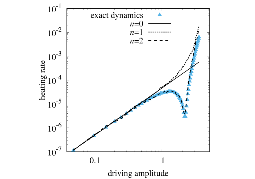
Figure 1: Heating rate in the classical spin system against the driving amplitude $\xi$. The system size is set to be $N=100$. Blue triangles show the heating rate estimated by exactly solving the equations of motion (15). The solid line, the dotted line, and the dashed line show the heating rates calculated by our formula (12) for $n=0$, 1, and 2, respectively. Error bars are smaller than the symbols.

Our numerical results are displayed in Fig. 1. The heating rate calculated by solving Eq. (15) shows non-monotonic behavior: the heating is suppressed for strong driving Ikeda and Polkovnikov (2021). On the other hand, for $n=0$ and 1, our formula (12) does not reproduce non-monotonicity. When $n=0$, our formula is reduced to the linear response expression, and hence the heating rate is proportional to $\xi^{2}$. When $n=1$, our formula agrees with the exact heating rate at weak and strong driving, but does not show non-monotonicity. We clearly see that our formula for $n=2$ well reproduces a curve of the exact heating rate, including characteristic non-monotonic behavior.

Frequency dependences of the heating rate are given in SM SM, in which we find that the non-monotonicity occurs at $\xi$ which is large but independent of $\omega$. Therefore, this non-monotonicity should be distinguished from dynamical freezing phenomena Das (2010); Haldar et al. (2018, 2021), in which heating is suppressed due to an emergent symmetry at ultra-strong driving with $\xi\propto\omega$.

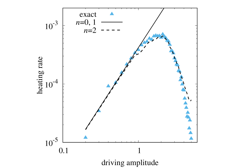
Figure 2: Heating rate in the quantum spin system against the driving amplitude $\xi$. Blue triangles show the heating rate estimated by exactly solving the Scrödinger equation for $N=16$. The solid line and the dashed line show the heating rates calculated by our formula (12) for $N=14$ with $n=0$ and 2, respectively (in the present model, $n=1$ gives an identical result to $n=0$). Error bars are smaller than the symbols.

Quantum model.— We also verify our formula in quantum systems. We consider a quantum spin-1/2 chain with the Hamiltonian

$$\left\{\begin{aligned} &H_{0}=-\sum_{i=1}^{N}[J_{z}\sigma_{i}^{z}\sigma_{i+1}^{z}+J_{x}\sigma_{i}^{x}\sigma_{i+1}^{x}+h\sigma_{i}^{z}],\\ &V(t)=-\xi\operatorname{\mathrm{sgn}}[\cos(\omega t)]\sum_{i=1}^{N}\sigma_{i}^{x},\end{aligned}\right.$$ (16)

where $\sigma^{\alpha}$ ($\alpha=x,y,z$) denotes the Pauli matrix. We fix $J_{z}=1$, $J_{x}=0.77$, $h=0.6$, and $T=0.5$ ($\omega\simeq 12.6$).

We prepare an initial state as a canonical thermal pure quantum state Sugiura and Shimizu (2013): we generate a random vector $\ket{r}$ whose elements are i.i.d. Gaussian of mean 0 and unit variance, and construct a state $\ket{\beta}=e^{-\beta H/2}\ket{r}/\braket{r}{e^{-\beta H}}{r}$. We then solve the Schrödinger equation $i\hbar d\ket{\psi(t)}/dt=H(t)\ket{\psi(t)}$ with $\ket{\psi(0)}=\ket{\beta}$, where we set $\hbar=1$ in numerical calculations. The heating rate is calculated in the same way as in classical systems: we measure $t_{1}$ and $t_{2}$ satisfying $t_{i}=\min_{n\in\mathbb{N}}\{t=nT:\braket{\psi(t)}{H_{0}}{\psi(t)}\geq N\varepsilon_{i}\}$ with $\varepsilon_{1}=-0.5$ and $\varepsilon_{2}=-0.48$ (the corresponding inverse temperature is $\beta\simeq 0.23$). The heating rate is given by $(\varepsilon_{2}-\varepsilon_{1})/(t_{2}-t_{1})$. For the system size $N=16$, we repeat the above procedure (the generation of an initial state, solving the Schrödinger equation, and measuring the heating rate) 10 times, and compute the average heating rate.

The heating rate is also evaluated for $N=14$ by using our formula with $n=0$ and 2 (in the present model, it is shown that $n=1$ gives the identical result to $n=0$). Details are explained in SM SM.

Numerical results are shown in Fig. 2. We can see that the heating rate again shows non-monotonic behavior, which implies that the system is not in the linear response regime. Our formula with $n=2$ reproduces this behavior.

Conclusion and Outlook.— We have derived a formula on the heating rate under fast driving with arbitrary driving strength. Our idea is based on considering the problem in a rotating frame in which driving looks weak. Such a rotating frame is found by using the high-frequency expansion of the micromotion operator. Our formulation is valid for both classical and quantum systems.

It is often argued that a truncation of the high-frequency expansion of the Floquet Hamiltonian describes dynamics in a prethermal regime before the heating takes place Mori et al. (2016); Kuwahara et al. (2016); Ikeda and Polkovnikov (2021), whereas an asymptotic divergent behavior of the high-frequency expansion is related to heating. Contrary to this argument, our formulation tells us that the information on heating under fast and strong periodic driving is encoded in a truncation of the high-frequency expansions of the Floquet Hamiltonian and the micromotion operator. Considering the micromotion operator is crucial in our formulation, although it is often neglected in investigating heating dynamics because of the fact that the micromotion describes fast oscillations rather than long-time slow dynamics.

Both in classical and quantum systems, we have found non-monotonic heating rates as a function of the driving amplitude. Such non-monotonicity has also been found in the previous study Ikeda and Polkovnikov (2021), and it looks universal in some extent. It is a future problem to understand universal features of the heating dynamics by using our formulation.

Some recent studies have also attempted to use aperiodic driving (random or quasiperiodic one) for controlling quantum many-body systems Nandy et al. (2017); Zhao et al. (2019); Crowley et al. (2020); Zhao et al. (2021); Long et al. (2021), and some rigorous results have begun to appear Else et al. (2020); Mori et al. (2021). It will be a fascinating open problem to give a simple and accurate heating-rate formula for fast and strong quasiperiodic driving.