Effect of an Attached End Mass in the Dynamics of Uncertainty Nonlinear Continuous Random System

Resumen

This work studies the dynamics of a one dimensional elastic bar with random elastic modulus and prescribed boundary conditions, say, fixed at one end, and attached to a lumped mass and two springs (one linear and another nonlinear) on the other extreme. The system analysis assumes that the elastic modulus has gamma probability distribution and uses Monte Carlo simulations to compute the propagation of uncertainty in this continuous–discrete system. After describing the deterministic and the stochastic modeling of the system, some configurations of the model are analyzed in order to characterize the effect of the lumped mass in the overall behavior of this dynamical system.

1 INTRODUCTION

The dynamics of a mechanical system depends on some parameters such as physical and geometrical properties, constraints, external and internal loading, initial and boundary conditions. Most of the theoretical models used to describe the behavior of a mechanical system assume nominal values for these parameters, such that the model gives one response for a given particular input. In this case the system is deterministic and its behavior is described by a single set of differential equations. However, in real systems they do not have a fixed value since they are subjected to uncertainties of measurement, imperfections in manufacturing processes, change of properties, etc. This variability in the set of system parameters leads to a large number of possible system responses for a given particular input. Now the system is stochastic and there is a family of differential equations sets (one for each realization of the random system) associated to it.

This work aims to study the propagation of uncertainty in the dynamics of a nonlinear continuos random system with a discrete element attached to it. In this sense, this work considers a one dimensional elastic bar, with random elastic modulus, fixed on the left extreme and with a lumped mass and two springs (one linear and another nonlinear) on the right extreme (fixed-mass-spring bar).

This paper is organized as follows. In section 2 is presented the deterministic modeling of the problem, the discretization procedure and the algorithm used to solve the equation of interest. The stochastic modeling of the problem is shown in section 3, as well as the construction of a probability distribution for the elastic modulus, using the maximum entropy principle, and a brief discussion on the Monte Carlo method. In section 4, some configurations of the model are analyzed in order to characterize the effect of lumped mass in the system dynamical behavior. Finally, in section 5, the main conclusions are emphasized and some directions for future work outlined.

2 DETERMINISTIC APPROACH

The continuous system of interest is the one-dimensional fixed-mass-spring bar shown in Figure 1.

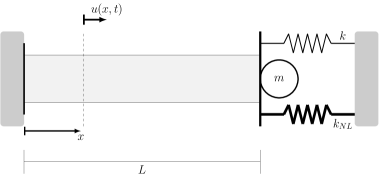
Figura 1: Sketch of a bar fixed at one and attached to two springs and a lumped mass on the other extreme.

2.1 Strong Formulation

The displacement of this system $\displaystyle u$ evolves according to the following partial differential equation

$$\rho A\mathinner{\dfrac{\partial{{}^{2}}u}{\partial{t^{2}}}}(x,t)+c\mathinner{\dfrac{\partial{}u}{\partial{t}}}(x,t)=\mathinner{\dfrac{\partial{}}{\partial{x}}}\left(EA\mathinner{\dfrac{\partial{}u}{\partial{x}}}(x,t)\right)+f(x,t),$$ (1)

which is valid for $\displaystyle 0<x<L$ and $\displaystyle 0<t<T$, being $\displaystyle L$ the bar unstretched length and $\displaystyle T$ a finite instant of time. In this equation $\displaystyle\rho$ is the mass density, $\displaystyle E$ is the elastic modulus, $\displaystyle A$ is the circular cross section area, $\displaystyle c$ is the damping coefficient, and $\displaystyle f(x,t)$ is an external force depending on position $\displaystyle x$ and instant $\displaystyle t$.

The left side of the bar is fixed at a rigid wall while the right side is attached to a lumped mass $\displaystyle m$ and two springs fixed to a rigid wall. The first spring (of stiffness $\displaystyle k$) is linear and exerts a restoring force proportional to the stretching on the bar. The second spring (of stiffness $\displaystyle k_{NL}$) is nonlinear and its restoring force is proportional to the cube of the stretching. The force which the lumped mass exerts on the bar is proportional to acceleration. These boundary conditions read as

$$u(0,t)=0\qquad\mbox{and}\qquad EA\mathinner{\dfrac{\partial{}u}{\partial{x}}}(L,t)=-ku(L,t)-k_{NL}\left[u(L,t)\right]^{3}-m\mathinner{\dfrac{\partial{{}^{2}}u}{\partial{t^{2}}}}(L,t)\mathchar 46\relax$$ (2)

Initially, any point $\displaystyle x$ of the bar presents displacement and a velocity respectively equal to

$$u(x,0)=u_{0}(x)\qquad\mbox{and}\qquad\mathinner{\dfrac{\partial{}u}{\partial{t}}}(x,0)=\dot{u}_{0}(x),$$ (3)

for $\displaystyle 0\leq x\leq L$. In these equations $\displaystyle u_{0}$ and $\displaystyle\dot{u}_{0}$ are given functions of position $\displaystyle x$.

Moreover, it is noteworthy that $\displaystyle u$ is assumed to be as regular as needed for the initial–boundary value problem of Eqs.(1), (2), and (3) to be well posed.

2.2 Variational Formulation

Let $\displaystyle\mathcal{U}_{t}$ be the class of (time dependent) basis functions and $\displaystyle\mathcal{W}$ be the class of weight functions. These sets are chosen as the space of functions with square integrable spatial derivative, which satisfy the essential boundary condition defined by Eq.(2).

The variational formulation of the problem under study says that one wants to find $\displaystyle u\in\mathcal{U}_{t}$ that satisfy, for all $\displaystyle w\in\mathcal{W}$, the weak equation of motion given by

$$\mathcal{M}(\ddot{u},w)+\mathcal{C}(\dot{u},w)+\mathcal{K}(u,w)=\mathcal{F}(w)+\mathcal{F}_{NL}(u,w),$$ (4)

where $\displaystyle\mathcal{M}$ is the mass operator, $\displaystyle\mathcal{C}$ is the damping operator, $\displaystyle\mathcal{K}$ is the stiffness operator, $\displaystyle\mathcal{F}$ is the external force operator, and $\displaystyle\mathcal{F}_{NL}$ is the nonlinear force operator. These operators are, respectively, defined as

$$\mathcal{M}(\ddot{u},w)=\int_{0}^{L}\left(\rho A\ddot{u}(x,t)w(x)\right)dx+m\ddot{u}(L,t)w(L),$$ (5)

$$\mathcal{C}(\dot{u},w)=\int_{0}^{L}c\dot{u}(x,t)w(x)dx,$$ (6)

$$\mathcal{K}(u,w)=\int_{0}^{L}\left(EAu^{\prime}(x,t)w^{\prime}(x)\right)dx+ku(L,t)w(L),$$ (7)

$$\mathcal{F}(w)=\int_{0}^{L}f(x,t)w(x)dx,$$ (8)

$$\mathcal{F}_{NL}(u,w)=-k_{NL}\left[u(L,t)\right]^{3}w(L),$$ (9)

where  $\displaystyle\dot{}$ is an abbreviation for temporal derivative and  ^′ is an abbreviation for spatial derivative.

The variational formulations for the initial conditions of Eq.(3), which are valid for all $\displaystyle w\in\mathcal{W}$, are respectively given by

$$\widetilde{\mathcal{M}}(u(\cdot,0),w)=\widetilde{\mathcal{M}}(u_{0},w),$$ (10)

and

$$\widetilde{\mathcal{M}}(\dot{u}(\cdot,0),w)=\widetilde{\mathcal{M}}(\dot{u}_{0},w),$$ (11)

where $\displaystyle\widetilde{\mathcal{M}}$ is the associated mass operator, defined as

$$\widetilde{\mathcal{M}}(u,w)=\int_{0}^{L}\rho Au(x,t)w(x)dx\mathchar 46\relax$$ (12)

2.3 An Eigenvalue Problem

Now consider the following generalized eigenvalue problem associated to Eq.(4),

$$-\nu^{2}\mathcal{M}(\phi,w)+\mathcal{K}(\phi,w)=0,$$ (13)

where $\displaystyle\nu$ is a natural frequency and $\displaystyle\phi$ is an associated mode shape.

In order to solve Eq.(13), the technique of separation of variables is employed, which leads to a Sturm-Liouville problem (Al Gwaiz, 2007), with denumerable number of solutions. Therefore, this generalized eigenvalue problem has a denumerable number of solutions, all of then such as the following eigenpair $\displaystyle(\nu_{n}^{2},\phi_{n})$, where $\displaystyle\nu_{n}$ is the $\displaystyle n$-th bar natural frequency and $\displaystyle\phi_{n}$ is the $\displaystyle n$-th bar mode shape.

It is important to observe that, the eigenfunctions $\displaystyle\{\phi_{n}\}_{n=1}^{+\infty}$ span the space of functions which contains the solution of the Eq.(13) (Brezis, 2010). As can be seen in Hagedorn DasGupta (2007), these eigenfunctions satisfy, for all $\displaystyle m\neq n$, the orthogonality relations given by

$$\mathcal{M}(\phi_{n},\phi_{m})=0,$$ (14)

and

$$\mathcal{K}(\phi_{n},\phi_{m})=0,$$ (15)

which made then good choices for the basis function when a weighted residual procedure (Finlayson Scriven, 1966) is used to approximate the solution of a nonlinear variational equation, such as Eq.(4).

2.4 Mode Shapes and Natural Frequencies

According to Blevins (1993), a fixed-mass-spring bar has its natural frequencies and the corresponding orthogonal modes shape given by

$$\nu_{n}=\lambda_{n}\frac{\bar{c}}{L},$$ (16)

and

$$\phi_{n}(x)=\sin{\left(\lambda_{n}\frac{x}{L}\right)},$$ (17)

where $\displaystyle\bar{c}=\sqrt{E/\rho}$ is the wave speed, and the $\displaystyle\lambda_{n}$ are the solutions of

$$\cot{\left(\lambda_{n}\right)}+\left(\frac{kL}{AE}\right)\frac{1}{\lambda_{n}}-\left(\frac{m}{\rho AL}\right)\lambda_{n}=0\mathchar 46\relax$$ (18)

The first six orthogonal modes shape of the fixed-mass-spring bar with $\displaystyle m=1{,}5~{}kg$, whose the other parameters are presented in the beginning of section 4, are illustrated in Figure 2. In this figure each sub-caption indicates the approximated natural frequency associated with the corresponding mode.

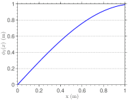
(a) $\displaystyle\nu_{1}\approx 0{,}07\times 10^{5}~{}rad/s$

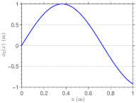
(b) $\displaystyle\nu_{2}\approx 0{,}22\times 10^{5}~{}rad/s$

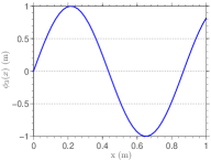
(c) $\displaystyle\nu_{3}\approx 0{,}37\times 10^{5}~{}rad/s$

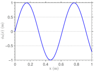
(d) $\displaystyle\nu_{4}\approx 0{,}52\times 10^{5}~{}rad/s$

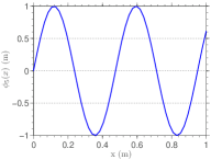
(e) $\displaystyle\nu_{5}\approx 0{,}67\times 10^{5}~{}rad/s$

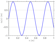
(f) $\displaystyle\nu_{6}\approx 0{,}83\times 10^{5}~{}rad/s$

Figura 2: The first six orthogonal modes shape and the corresponding (approximated) natural frequencies of a fixed-mass-spring bar with $\displaystyle m=1{,}5~{}kg$.

2.5 Galerkin Formulation

In order of approximate the solution of Eqs.(4), (10) and (11) the Galerkin method (Hughes, 2000) is employed. Therefore, the displacement field $\displaystyle u$ is approximated by a linear combination of the form

$$u^{N}(x,t)=\sum_{n=1}^{N}u_{n}(t)\phi_{n}(x),$$ (19)

where the basis functions $\displaystyle\phi_{n}$ are the orthogonal modes shape of the fixed-mass-spring bar, exemplified in the end of section 2.4, and the coefficients $\displaystyle u_{n}$ are time-dependent functions. For a reason that will be clear soon, define $\displaystyle\mathbf{u}(t)$ of $\displaystyle\mathbb{R}^{N}$ as the vector in which the $\displaystyle n$-th component is $\displaystyle u_{n}(t)$.

Since $\displaystyle u^{N}$ is not a solution of Eq.(4), when the field $\displaystyle u$ is approximated by $\displaystyle u^{N}$ a residual function is obtained. This residual function is orthogonally projected into the vector space spanned by the functions $\displaystyle\{\phi_{n}\}_{n=1}^{N}$ in order to minimize the error incurred by the approximation (Hughes, 2000). This procedure results in the following $\displaystyle N\times N$ set of nonlinear ordinary differential equations

$$\left[M\right]\ddot{\mathbf{u}}(t)+\left[C\right]\dot{\mathbf{u}}(t)+\left[K\right]\mathbf{u}(t)=\mathbf{f}(t)+\mathbf{f}_{NL}\left(\mathbf{u}(t)\right),$$ (20)

supplemented by the following pair of initial conditions

$$\mathbf{u}(0)=\mathbf{u}_{0}\qquad\mbox{and}\qquad\mathbf{\dot{u}}(0)=\mathbf{\dot{u}}_{0}\mathchar 46\relax$$ (21)

where $\displaystyle\left[M\right]$ is the mass matrix, $\displaystyle\left[C\right]$ is the damping matrix, $\displaystyle\left[K\right]$ is the stiffness matrix, and the upper dot again denotes the time derivative. Also, $\displaystyle\mathbf{f}(t)$, $\displaystyle\mathbf{f}_{NL}\left(\mathbf{u}(t)\right)$, $\displaystyle\mathbf{u}_{0}$, and $\displaystyle\mathbf{\dot{u}}_{0}$ are vectors of $\displaystyle\mathbb{R}^{N}$, which respectively represent the external force, the nonlinear force, the initial position, and the initial velocity.

The initial value problem of Eqs.(20) and (21) has its solution approximated by Newmark method (Newmark, 1959). The reader interested in details about this integration scheme is encouraged to see Hughes (2000).

3 STOCHASTIC APPROACH

3.1 Probabilistic Model

Consider a probability space $\displaystyle(\Omega,{\mathbb{A}},{\mathbb{P}})$, where $\displaystyle\Omega$ is sample space, $\displaystyle{\mathbb{A}}$ is a $\displaystyle\sigma$-field over $\displaystyle\Omega$ and $\displaystyle{\mathbb{P}}$ is a probability measure. In this probabilistic space, the elastic modulus is assumed to be a random variable $\displaystyle E\mathrel{\mathop{\mathchar 58\relax}}\Omega\to\mathbb{R}$ that associates to each event $\displaystyle\omega\in\Omega$ a real number $\displaystyle E(\omega)$. Consequently, the displacement of the bar is the random field $\displaystyle U\mathrel{\mathop{\mathchar 58\relax}}[0,L]\times[0,T]\times\Omega\to\mathbb{R}$, which evolves according the following stochastic partial differential equation

$$\rho A\mathinner{\dfrac{\partial{{}^{2}}U}{\partial{t^{2}}}}(x,t,\omega)+c\mathinner{\dfrac{\partial{}U}{\partial{t}}}(x,t,\omega)=\mathinner{\dfrac{\partial{}}{\partial{x}}}\left(E(\omega)A\mathinner{\dfrac{\partial{}U}{\partial{x}}}(x,t,\omega)\right)+f(x,t),$$ (22)

being the partial derivatives now defined in the mean square sense (Papoulis Pillai, 2002). This problem has boundary and initial conditions similar to those defined in Eqs.(2) and (3), by changing $\displaystyle u$ for $\displaystyle U$ only.

3.2 Elastic Modulus Distribution

The elastic modulus cannot be negative, so it is reasonable to assume the support of random variable $\displaystyle E$ as the interval $\displaystyle(0,+\infty)$. Therefore, the probability density function (PDF) of $\displaystyle E$ is a nonnegative function $\displaystyle p_{\tiny{E}}\mathrel{\mathop{\mathchar 58\relax}}(0,+\infty)\to\mathbb{R}$, which respects the following normalization condition

$$\int_{0}^{+\infty}p_{\tiny{E}}(\xi)d\xi=1\mathchar 46\relax$$ (23)

Also, the mean value of $\displaystyle E$ is known real number $\displaystyle\mu_{E}$, i.e.,

$$\mathbb{E}\left[E\right]=\mu_{E},$$ (24)

where the expected value operator of $\displaystyle E$ is defined as

$$\mathbb{E}\left[E\right]=\int_{0}^{+\infty}E(\xi)p_{\tiny{E}}(\xi)d\xi$$ (25)

Finally, one also wants that $\displaystyle E$ has finite variance, i.e.,

$$\mathbb{E}\left[\left(E-\mu_{E}\right)^{2}\right]<+\infty,$$ (26)

which is possible (Soize, 2000), for example, if

$$\mathbb{E}\left[\ln\left(E\right)\right]<+\infty\mathchar 46\relax$$ (27)

Following the suggestion of Soize (2000), the maximum entropy principle (Shannon, 1948; Jaynes, 1957a, b) is employed in order to consistently specify $\displaystyle p_{\tiny{E}}$. This methodology chooses for $\displaystyle E$ the PDF which maximizes the differential entropy function, defined by

$$\mathbb{S}\left[p_{\tiny{E}}\right]=-\int_{0}^{+\infty}p_{\tiny{E}}(\xi)\ln\left[p_{\tiny{E}}(\xi)\right]d\xi,$$ (28)

subjected to (23), (24), and (27), the restrictions that effectively define the known information about $\displaystyle E$.

Respecting the constraints imposed by (23), (24), and (27), the PDF that maximizes Eq.(28) is given by

$$p_{\tiny{E}}(\xi)=\mathds{1}_{(0,+\infty)}\frac{1}{\mu_{E}}\left(\frac{1}{\delta_{E}^{2}}\right)^{\left(\displaystyle\frac{1}{\delta_{E}^{2}}\right)}\frac{1}{\Gamma(1/\delta_{E}^{2})}\left(\frac{\xi}{\mu_{E}}\right)^{\left(\displaystyle\frac{1}{\delta_{E}^{2}}-1\right)}\exp\left(-\frac{\xi}{\delta_{E}^{2}\mu_{E}}\right),$$ (29)

where $\displaystyle\mathds{1}_{(0,+\infty)}$ denotes the indicator function of the interval $\displaystyle(0,+\infty)$, $\displaystyle\delta_{E}$ is the dispersion factor of $\displaystyle E$, and $\displaystyle\Gamma$ indicates the gamma function. This PDF is a gamma distribution.

3.3 Stochastic Solver: Monte Carlo Method

Uncertainty propagation in the stochastic dynamics of the continuous–discrete system under study is computed by Monte Carlo (MC) method (Metropolis Ulam, 1949). This stochastic solver uses a Mersenne twister pseudorandom number generator (Matsumoto Nishimura, 1998), to obtain many realizations of the random variable $\displaystyle E$. Each one of these realizations defines a new Eq.(4), so that a new variational problem is obtained. After that, these new variational problems are solved deterministically, such as in section 2.5. All the MC simulations reported in this work use $\displaystyle 4^{5}$ samples to access the random system. Further details about MC method can be seen in Liu (2001); Shonkwiler Mendivil (2009); Robert Casella (2010).

4 NUMERICAL EXPERIMENTS

The numerical experiments presented in this section adopt the following deterministic parameters for the studied system: $\displaystyle\rho=7900~{}kg/m^{3}$, $\displaystyle c=10~{}kNs/m$, $\displaystyle A=625\pi~{}mm^{2}$, $\displaystyle k=650~{}N/m$, $\displaystyle k_{NL}=650\times 10^{13}~{}N/m^{3}$, $\displaystyle L=1~{}m$, and $\displaystyle T=8~{}ms$. Besides that, four values for the lumped mass are considered: $\displaystyle m=1{,}5,~{}7{,}5,~{}15,~{}\mbox{and}~{}75~{}kg$. The random variable $\displaystyle E$, is characterized by $\displaystyle\mu_{E}=203~{}GPa$ and $\displaystyle\delta_{E}=10\leavevmode\,\%{}$.

The initial conditions for displacement and velocity are respectively given by

$$u_{0}=\alpha_{1}\phi_{3}(x)+\alpha_{2}x,\qquad\mbox{and}\qquad\dot{u}_{0}=0,$$ (30)

where $\displaystyle\alpha_{1}=0{,}1~{}mm$ and $\displaystyle\alpha_{2}=0{,}5\times 10^{-3}$. Note that $\displaystyle u_{0}$ reaches the maximum value at $\displaystyle x=L$. This function is used to “activate"the spring cubic nonlinearity, which depends on the displacement at $\displaystyle x=L$.

The time-dependent external force acting on the system has the form of a sine wave with circular frequency equal to the first natural frequency

$$f(x,t)=\sigma\phi_{1}(x)\sin{\left(\nu_{1}t\right)},$$ (31)

where the external force amplitude is $\displaystyle\sigma=1~{}N$.

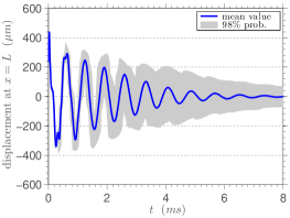
(a) $\displaystyle\rho AL/m\approx 10$

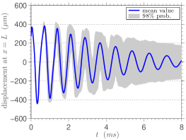
(b) $\displaystyle\rho AL/m\approx 2$

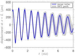
(c) $\displaystyle\rho AL/m\approx 1$

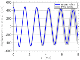
(d) $\displaystyle\rho AL/m\approx 0{,}2$

Figura 3: This figure illustrates the mean value (blue line) and a 98 % of probability interval of confidence (grey shadow) for the random process $\displaystyle U(L,\cdot,\cdot)$, for several values of the continuous–discrete mass ratio.

4.1 Analysis of Random System Envelope of Reliability and Phase Space

The mean value of $\displaystyle U(L,\cdot,\cdot)$ and an envelope of reliability, wherein a realization of the stochastic system has 98 % of probability of being contained, are shown, for different values of the continuous–discrete mass ratio $\displaystyle\rho AL/m$, in Figure 3. By observing this figure one can note that, as the value of lumped mass increases, the decay of the system displacement amplitude decreases significantly. This indicates that this continuous–discrete system is not much influenced by damping for small values of the continuous–discrete mass ratio.

The mean phase space of the fixed-mass-spring bar at $\displaystyle x=L$ is shown, for different values of the continuous–discrete mass ratio, in Figure 4. The observation made in the previous paragraph can be confirmed by analyzing this figure, since the system mean orbit tends from a stable focus to an ellipse as the continuous–discrete mass ratio decreases. In other words the limiting behavior of the system when $\displaystyle\rho AL/m\to 0^{+}$ is a mass-spring system.

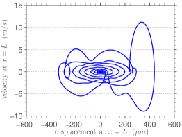
(a) $\displaystyle\rho AL/m\approx 10$

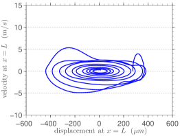
(b) $\displaystyle\rho AL/m\approx 2$

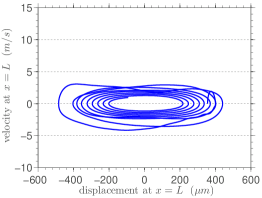
(c) $\displaystyle\rho AL/m\approx 1$

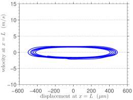
(d) $\displaystyle\rho AL/m\approx 0{,}2$

Figura 4: This figure illustrates the mean value of the fixed-mass-spring bar phase space at $\displaystyle x=L$, for several values of the continuous–discrete mass ratio.

4.2 Analysis of Random System PDF

The difference between the system dynamical behavior, for different values of $\displaystyle m$, is even clearer if one looks to the PDF estimations of the (normalized) random variable $\displaystyle U(L,T,\cdot)$, which are presented in Figure 5. For large values of the continuous–discrete mass ratio, the PDF of $\displaystyle U(L,T,\cdot)$ displays bimodal shape, which tends to a unimodal shape as the lumped mass grows, i.e., the continuous–discrete mass ratio decreases. Furthermore, it can be noted that when $\displaystyle\rho AL/m\approx 1$ the greatest probability occurs around the mean value of $\displaystyle U(L,T,\cdot)$.

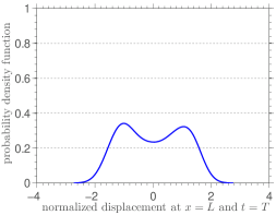
(a) $\displaystyle\rho AL/m\approx 10$

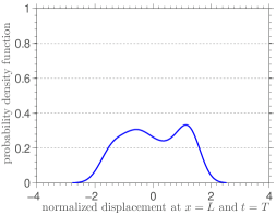
(b) $\displaystyle\rho AL/m\approx 2$

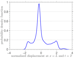
(c) $\displaystyle\rho AL/m\approx 1$

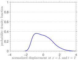
(d) $\displaystyle\rho AL/m\approx 0{,}2$

Figura 5: This figure illustrates estimations to the PDF of the (normalized) random variable $\displaystyle U(L,T,\cdot)$, for several values of the continuous–discrete mass ratio.

5 CONCLUDING REMARKS

A model to describe the dynamics of fixed-mass-spring bar with a random elastic modulus is presented. The aleatory parameter is modeled as a random variable with gamma distribution, being the probability distribution of this parameter obtained by the principle of maximum entropy. The paper analyzes some configurations of the model to order to characterize the effect of the lumped mass in the overall behavior of this dynamical system. This analysis shows that the dynamics of the random system is significantly altered when the values of the lumped mass are varied.

6 ACKNOWLEDGMENTS

The authors are indebted to Brazilian Council for Scientific and Technological Development (CNPq), Coordination of Improvement of Higher Education Personnel (CAPES), and Foundation for Research Support in Rio de Janeiro State (FAPERJ) for the financial support.