Fleet Sizing and Allocation for On-demand Last-Mile Transportation Systems

Abstract

The last-mile problem refers to the provision of travel service from the nearest public transportation node to home or other destination. Last-Mile Transportation Systems (LMTS), which have recently emerged, provide on-demand shared transportation. In this paper, we investigate the fleet sizing and allocation problem for the on-demand LMTS. Specifically, we consider the perspective of a last-mile service provider who wants to determine the number of servicing vehicles to allocate to multiple last-mile service regions in a particular city. In each service region, passengers demanding last-mile services arrive in batches, and allocated vehicles deliver passengers to their final destinations. The passenger demand (i.e., the size of each batch of passengers) is random and hard to predict in advance, especially with limited data during the planning process. The quality of fleet-allocation decisions is a function of vehicle fixed cost plus a weighted sum of passenger’s waiting time before boarding a vehicle and in-vehicle riding time. We propose and analyze two models—a stochastic programming model and a distributionally robust optimization model—to solve the problem, assuming known and unknown distribution of the demand, respectively. We conduct extensive numerical experiments to evaluate the models and discuss insights and implications into the optimal fleet sizing and allocation for the on-demand LMTS under demand uncertainty.

1 Introduction

The last-mile problem refers to the design and provision of travel services from a public transportation node to a passenger’s final destination. It is a fundamental practical problem that has attracted intense attention in the past decade for several reasons. First, governments worldwide are under pressure to increase public transport’s share of urban trips to reduce road congestion and air pollution. Maybe not surprisingly, urban planners recently recognized that the unavailability of last-mile services is one of the main deterrents to the use of public transport. Second, the aging of populations has increased the demand for such services. Third, more countries impose legal requirements to ensure adequate mobility for particular demographic groups, who are most likely to need last-mile services, such as people with physical disabilities.

Any passenger needing on-demand last-mile service may provide advance notice to the last-mile transportation systems (LMTS) of his/her impending arrival at the alighting station and her specific final destination. Once this information is received, the LMTS assigns the passenger to one of the vehicles in the LMTS fleet, plans the vehicle’s route so that it includes a stop at the passenger’s destination, estimates the vehicle’s departure time, and notifies the passenger accordingly. Once all of the passengers assigned to a vehicle are on board, the vehicle executes a delivery route with stops at each passenger’s destination and returns to the station to pick up passengers for its next delivery tour. Many papers address various models and case studies of LMTS. With the high penetration of services such as Uber worldwide, most people are aware of the benefits of on-demand transportation services and request even more specialized forms, including last-mile service (Wang and Yang (2019)) .

In this paper, we investigate the fleet sizing and allocation problem for the on-demand LMTS. Specifically, we consider the perspective of a last-mile service provider who wants to determine the number of servicing vehicles to allocate to multiple service regions in a particular city. In each service region (e.g., an area around a metro station), passengers demanding last-mile services arrive in batches (e.g., as a result of consecutive arrivals of metros or trains), and allocated vehicles deliver passengers to their final destinations, i.e., last-mile stops. The size of each batch of passengers (demand henceforth) is random and hard to predict in advance. The quality of fleet-allocation decisions is a function of vehicle fixed cost (vehicle rental or purchase cost) plus a weighted sum of passenger waiting time before boarding a vehicle and in-vehicle riding time.

The fleet sizing and allocation problem is challenging, especially since the practical passenger demand is stochastic (i.e., uncertain). If we know the exact probability distribution of random demand, we may formulate the problem as a two-stage stochastic programming model. In the first stage, we decide the number of vehicles to allocate to each service region and their routes before the realization of random demand. Then in the second stage, we observe the realizations of stochastic demands and make optimal recourse actions (assigning passengers to vehicles), conditioning on first-stage decisions, and accordingly compute the associated passenger waiting and riding times. Mathematically, the stochastic programming model identifies vehicle allocation and routing decisions that minimize the total cost, comprising the fixed cost of vehicle allocation and the expected weighted sum of waiting time and riding time for passengers, where the expectation is taken with respect to this known probability distribution of random demand.

In reality, it is often notoriously difficult to accurately estimate the exact probability distribution of demand, especially with limited data during the planning stage. LMTS is a relatively emerging transportation mode, and thus sufficient data on LMTS operations is not readily available. Even if LMTS companies collect data on their LMTS operations, the data may not be sufficient or have high quality to model the demand distribution. Moreover, it is challenging to obtain LMTS data from companies due to privacy issues, among others. If we calibrate a stochastic programming model to a data sample from a biased distribution of random demand, then the resulting biased optimal decisions may demonstrate disappointing out-of-sample performance (in terms of passenger waiting and riding times) under the true distribution– a phenomenon known as optimizer’s curse (see Esfahani and Kuhn (2018) and Smith and Winkler (2006) for a detailed discussion). Alternatively, one can construct an ambiguity set (i.e., a family) of all plausible probability distributions compatible with the available limited data or expert knowledge about demand.

In this paper, we address the uncertainty of passengers’ demand for last-mile service. We propose, analyze, and evaluate the computational and operational performance of two models for the fleet sizing and allocation problem, assuming known and unknown distribution of the demand, respectively. First, a stochastic programming model is proposed to minimize the fixed cost of allocated vehicles and the expectation of a weighted sum of passenger waiting and riding times, under a distributional belief of demand. Second, a distributionally robust model is proposed to minimize the fixed cost of vehicles and the worst-case (i.e., maximum) expectation of passenger waiting time and riding times; we also evaluate the worst-case expectation over an ambiguity set (i.e., a family of all possible distributions of uncertain demand) and characterize the ambiguity set by known mean and support information of demand. We conduct extensive numerical experiments and discuss the insights and implications by examining trade-offs between total cost, fleet size, and passenger waiting and riding times.

The proposed model generalizes the single-service region LMTS routing and scheduling formulation in literature by (1) considering multiple service regions, (2) considering fleet sizing and allocation decisions, and (3) incorporating the uncertainty of passenger demand. To the best of our knowledge, and according to our literature review in Section 2, this is the first paper that provides a theoretical and computational analysis of stochastic optimization models for the fleet sizing and allocation problem for LMTS.

The reminder of the paper is structured as follows. In Section 2, we review the relevant literature. In Section 3, we formally define the problem and propose two model formulations. In Section 4, we present computational results and discuss managerial implications. Finally, we draw conclusions and discuss future directions in Section 5.

2 Relevant Literature

Existing literature has addressed various models and case studies of the LMTS. Several case studies analyze LMTS in different contexts, including Liu et al. (2012)’s study of a bicycle-sharing program for a passenger LMTS in Beijing. Some studies have examined the design and performance evaluation of an LMTS from a planning perspective. For example, Wang and Odoni (2016) address the planning side by focusing on passenger LMTS from a stochastic and planning perspective and provide closed-form approximations for the performance of an LMTS as a function of the system’s fundamental design parameters. Zhu et al. (2020) study passengers’ multi-modal commuting behavior with ride-splitting and ride-sourcing systems, while considering their feeding effects on public transit—i.e., the ride-splitting fleet provides first- and last-mile services to public transit.

Recent studies have examined the operation of an LMTS from an optimization perspective. For example, Wang (2019) focuses on LMTS from an operational perspective and provides efficient strategies for passenger assignment, vehicle routing, and scheduling operations based on a set of last-mile demand information. Similarly, Agussurja et al. (2019) study the use of ride-sharing in satisfying last-mile demands with the assumption that last-mile demands are uncertain and come in batches, and propose a two-level Markov decision process framework that is capable of generating a vehicle-dispatching policy. Liu et al. (2019) focus on the fleet size and scheduling of feeder transit services while considering the influence of bike-sharing systems, propose several hybrid operation modes that combine fixed and dynamic frequencies in a bimodal period, and compare these with conventional bus scheduling with constant service frequencies. Chen et al. (2020a) focus on solving the first-mile ride-sharing problem using autonomous vehicles and propose a mixed-integer linear programming model to determine autonomous vehicle dispatch and ride-sharing schemes for minimum operational costs. Serra et al. (2019) study the scheduling problem of last-mile service while considering uncertainty in the system, and propose a two-stage stochastic programming formulation for scheduling a set of known passengers and uncertain passengers that is realized from a finite set of scenarios. Chen and Wang (2018a, b) study the pricing problem of multiple types of passengers in a LMTS using a queueing model to approximate passenger waiting time.

Personal rapid transit (PRT) and demand responsive transit (DRT), which refer to a variety of on-demand transportation systems with characteristics that are similar, in some ways, to LMTS, have also attracted significant attention in recent years. For instance, the PRT system control frameworks by Anderson (1998); financial assessments by Bly and Teychenne (2005) and Berger et al. (2011); performance approximations by Lees-Miller et al. (2009); and case studies by Mueller and Sgouridis (2011). Other papers focus on DRT concept discussions, practical implementation, and assessment of simulations in case studies, such as Horn (2002) and Quadrifoglio et al. (2008), among others. Relevant fleet sizing problems have also been studied for on-demand ride-pooling service by Ke et al. (2020); one-way car sharing service by Xu and Meng (2019); and autonomous electric vehicles considering charging system planning by Zhang et al. (2019).

In contrast to the increased awareness for LMTS modeling and methodology research, the availability of practical datasets is a limiting factor in LMTS research. In our numerical study, we construct a real case study based on New York City’s travel demand data. In another paper, Hao et al. (2021) curated last-mile transportation demand data arising from job-related commute in the United States, with an emphasis on the correlation between last-mile demand and household income level.

For the challenge of stochastic and uncertain demand, we refer to some frameworks for optimization under uncertainty: stochastic programming, robust optimization, and distributionally robust optimization. When using stochastic programming, the goal is to optimize a certain measure of a random outcome (e.g., the expected operational cost) for a given fully known distribution of the uncertain parameters. We refer to Birge and Louveaux (2011) and Shapiro et al. (2014) and references therein for thorough discussions about applications, formulations, and solution algorithms. Robust optimization (RO) assumes complete ignorance about the probability distribution of uncertain parameters. Instead, it assumes that an uncertain parameter’s values may vary in a given constrained set, called “uncertainty set” (Ben-Tal et al., 2015; Bertsimas and Sim, 2004; Soyster, 1973). Optimization is performed with respect to the worst-case scenario in the uncertainty set, which may inevitably lead to over-conservatism and suboptimal decisions for other more-likely scenarios (Chen et al., 2020b; Delage and Ye, 2010; Thiele, 2010). By focusing on the worst-case scenario, RO solutions are often overly conservative. Moreover, they usually have poor expected performances because they cannot capture the distributional information of uncertainty. Distributionally robust optimization (DRO) is a third approach to model uncertainty that bridge the gap between the conservatism of RO and the specificity of SP. DRO optimal solutions are sought for the worst-case probability distribution within a family of candidate distributions, called an “ambiguity set”. One can use easy-to-approximate information such as the mean and range of random parameters to construct the ambiguity sets and models that better mimic reality and are less conservative than RO models. In addition, DRO models with some types of carefully designed ambiguity sets are often more tractable than their SP counterparts (Delage and Ye, 2010; Rahimian and Mehrotra, 2019).

3 Formulation and Analysis

In this section, we formally define the fleet sizing and allocation problem for the on-demand LMTS. We propose and analyze two optimization models, namely, a two-stage stochastic mixed-integer linear programming model in Section 3.2 and a two-stage distributionally robust model in Section 3.3.

3.1 Definitions and Random Parameters

We consider the perspective of a last-mile service provider who wants to determine the number of vehicles $m_{s}$ to allocate to each service region $s\in S$ (e.g., an area around a metro station) in a particular city. Each service region $s\in S$ consists of a known number of last-mile stops $J_{s}$. For each stop $j\in J_{s}$ there is a known number, $K_{s}$, of feasible vehicle routes (i.e., a sequence of last-mile stops that a vehicle should visit on a trip). In each planing period (i.e., morning, afternoon, etc.), a set of punctual $I_{s}$ trains arrive at each service region $s\in S$. Each train dispatches a batch of passengers demanding last-mile service, and allocated vehicles deliver them to their final last-mile destinations. The number of passengers (demand henceforth) that need rides to each last-mile stop $j\in J_{s}$ is random. The randomness of the demand stems from the uncertain number of passengers who make a last-minute request for last-mile service, in addition to those who request their last-mile service in advance. We make the following assumptions as in Wang (2019):

Table 1: Notation.

Indices
$i$	index of train
$j$	index of last-mile stop
$k$	index of route
Sets
$S$	set of service regions
$K_{s}$	set of pre-selected feasible routes in service region $s$
$I_{s}$	set of trains arriving to bring passengers in sequence in service region $s$
$J_{s}$	set of pre-specified last-mile stops in service region $s$
Parameters
$M$	maximum total number of vehicles in the fleet
$n_{i,j,s}$	(random) number of passengers demanding last-mile stop $j$ arriving at the station from train $i$
$\underline{n}_{i,j,s}/\overline{n}_{i,j,s}$	lower/upper bound of $n_{i,j,s}$
$\phi_{j,k}$	1 if last-mile stop $j$ is served by route $k$; 0 otherwise
$t_{k}$	total travel time of route $k$, in terms of intervals between arrival trains
$t_{j,k}$	travel time to last-mile stop $j$ on route $k$
$c$	vehicle capacity (i.e., number of seats) for vehicle
$h$	inter-arrival time (headway) between trains (demand batches)
$f_{s}$	fixed cost of each vehicle
$\beta^{\mbox{\tiny w}}$	weight of passenger waiting time before boarding in the objective function
$\beta^{\mbox{\tiny r}}$	weight of passenger in-vehicle riding time in the objective function
Decision variables
$m_{s}$	number of vehicles allocated to service region $s$
$z_{i,j,k,s}$	number of passengers with destination at last-mile stop $j$ assigned to route $k$ right after arrival of train $i$
$w_{i,k,s}$	number of trips on route $k$ starting right after arrival of train $i$
Intermediate variables
$u_{i,j,s}$	number of unserved passengers with destination at last-mile stop $j$ waiting at the station
	after the arrival of train $i$
$v_{i,s}$	number of available vehicles at the station after the arrival of train $i$ in service region $s$
	and its corresponding service assignment

• The delivery fleet consists of at most $M$ vehicles, each with integer capacity $c$;

• The set of last-mile stops in each service region is finite;

• The set of feasible routes for LMTS vehicles in each service region is finite and preselected based on geometry, historical demand patterns, and some practical constraints—e.g., limits on the maximum number of last-mile stops on a single route or the route’s maximum travel distance or travel time;

• The inter-arrival time (headway) between arrival trains is deterministic and equal to $h$.

Given a fleet of at most $M$ vehicles and the sets of last-mile stops and preselected routes for LMTS vehicles, we aim to identify: (1) the number of vehicles to allocate for each service region, (2) a routing plan for the allocated vehicles (i.e., route selection) in each service region, and (3) the assignment of passengers to vehicles for different realizations of demand patterns. Decisions (1)–(2) are first-stage decisions that we make before observing demand patterns. If a route is selected, a vehicle should visit all of the last-mile stops specified on this route. The assignment decisions (3) represent the recourse actions in response to the first-stage decisions and the realizations of demand patterns. The quality of fleet-allocation decisions is a function of the vehicle fixed cost (which may include vehicle rental or purchase cost, etc.) plus a weighted sum of passenger waiting time before boarding a vehicle and in-vehicle riding time.

General notation: For $a,b\in\mathbb{Z}$, we define $[a]:=\{1,2,\ldots,a\}$ and $[a,b]_{\mathbb{Z}}:=\{c\in\mathbb{Z}:a\leq c\leq b\}$. The abbreviations “w.l.o.g.” and “w.l.o.o.” respectively, represent “without loss of generality” and “without loss of optimality.” For notation brevity, we use ($I_{s}$, $J_{s}$, $K_{s}$) to denote both the number and set of (trains, last-mile stops, routes) in service region $s$. For notational and modeling convenience, we assume w.l.o.g. that last-mile stops (and routes) are numbered sequentially, e.g., $J_{1}:=\{1,\ldots,4\}$, $J_{2}:=\{5,\ldots,10\}$, $K_{1}:=\{1,2,3\}$, $K_{2}:=\{4,5,6,7\}$, etc.

3.2 Two-stage Stochastic Model (SP) for Fleet Sizing and Allocation

In this section, we assume that we know the joint probability distribution $\mathbb{P}$ of the random number of passengers arriving at the station from train $i$ with a destination of last-mile stop $j$ in each service region $s$, $n_{i,j,s}$, for all $s\in S,\ i\in I_{s}$ and $j\in J_{s}$ and formulate the problem as a two-stage a “prior” stochastic mixed-integer programming model (SP). In the first stage, we determine the number of vehicles to allocate to each service region, their routes, and the number of trips on each route. In the second stage, we assign passengers to vehicles for different realizations of demand and compute the associated riding and waiting-time costs for passengers. A priori optimization has a managerial advantage, since it guarantees the regularity of service, which is beneficial for both passengers and the service provider.

Let integer decision variable $m_{s}$ represent the number of vehicles allocated to service region $s$. The feasible region $\mathcal{M}$ of variables $m$ is defined in (2) such that the number of allocated vehicles is less than or equal to the total number of vehicles in the fleet:

$$\mathcal{M} =\left\{m:\begin{array}[]{l}\sum_{s\in S}m_{s}\leq M.\end{array}\right\}$$ (2)

Let variable $w_{i,k,s}$ represent the number of trips on route $k$ starting right after the arrival of train $i$ at service region $s$, for all $i,k,s$. Let variable $v_{i,s}$ represent the number of vehicles waiting at the metro station after arrival of the train (demand batch) $i$ in service region $s$, for all $i,k,s$. Feasible region $\mathcal{W}$ of $(w,v)$ in (6) defines and constrains the number of vehicles waiting at each metro station $s$ after the arrival of each train $i$ (demand batch) and its corresponding service assignment.

$$\mathcal{W} =\left\{(v,w):\begin{array}[]{l}v_{0,s}=m_{s}-\sum\limits_{k\in K_{s}}w_{0,k,s},\ \forall s\in S\\ v_{i,s}=v_{i-1,s}+\sum\limits_{k\in K_{s}}w_{i-t_{k},k,s}-\sum\limits_{k\in K_{s}}w_{i,k,s},\ \forall s\in S,\ \forall{\color[rgb]{0,0,0}i\in I_{s}\setminus\{0\}}\\ v_{i,s}\geq 0,\ w_{i,k,s}\in\mathbb{Z}_{,}\ \forall(i,j,k,s)\end{array}\right\}$$ (6)

Given a feasible $m\in\mathcal{M}$, $w\in\mathcal{W}$, and a joint realization of uncertain parameters $\xi:=(n_{i,j,s})$, we can compute: (1) the number of passengers $z_{i,j,k,s}$ with a destination of last-mile stop $j$ assigned to route $k$ right after the arrival of train $i$ at service region $s$, and (2) the number of unserved passengers $u_{i,j,s}$ with a destinations of each last-mile stop $j$ waiting at the metro station after the arrival of train (demand batch) $i$ at service region $s$ and its corresponding service assignment using the following linear program (see Table 1 for notation):

$$Q(m,w,\xi):= \min\ \beta^{\mbox{\tiny w}}\sum\limits_{s\in S}\sum\limits_{i\in I_{s}}\sum\limits_{j\in J_{s}}hu_{i,j,s}+\beta^{\mbox{\tiny r}}\sum\limits_{s\in S}\sum\limits_{i\in I_{s}}\sum\limits_{j\in J_{s}}\sum\limits_{k\in K_{s}}t_{j,k}z_{i,j,k,s}$$ (7a)

$$\ \ \text{s.t.}\ u_{0,j,s}=n_{0,j,s}-\sum\limits_{k\in K_{s}}z_{0,j,k,s}\phi_{j,k},\forall s\in S,\ \forall j\in J_{s}$$ (7b)

$${\color[rgb]{0,0,0}u_{i,j,s}=u_{i-1,j,s}+n_{i,j,s}-\sum\limits_{k\in K_{s}}z_{i,j,k,s}\phi_{j,k},\forall s\in S,\ \forall i\in I_{s}\setminus\{0\},\ \forall j\in J_{s}}$$ (7c)

$$\sum\limits_{j\in J_{s}}z_{i,j,k,s}\phi_{j,k}\leq cw_{i,k,s},\ \forall s\in S,\ \forall i\in I_{s},\ \forall k\in K_{s}$$ (7d)

$$\ u_{i,j,s}\geq 0,\ z_{i,j,k,s}\geq 0,\ \forall(i,j,k,s)$$ (7e)

The objective function (7a) minimizes a linear cost function of the total waiting time and riding time for passengers. Constraints (7b) and (7c) are passenger flow constraints—i.e., they define and constrain the number of unserved passengers with a destinations of each last-mile stop who are waiting at the metro station after the arrival of train $i_{s}$ and its corresponding service assignment. Constraint (7d) ensures the vehicle service capacity restriction. Finally, constraint (7e) specifies the feasible ranges of the decision variables. Accordingly, we formulate the stochastic fleet sizing and allocation of fleet problem as follows:

$$\min\limits_{m\in\mathcal{M},w\in\mathcal{W}}\Big{(}\sum_{s\in S}f_{s}m_{s}+\ \mathbb{E}_{\mathbb{P}}[Q(m,w,\xi)]\Big{)}$$ (8)

The SP formulation in (8) searches for vehicle sizing, allocation, routing, and scheduling decisions that minimize the vehicle fixed cost plus a weighted expected sum of passenger waiting time and riding time, where the expectation is taken with respect to a known joint probability distribution $\mathbb{P}$ of $\xi$, where $\xi$ is the a vector of demand (i.e., a vector of all $(n_{i,j,s}),$ for all $s\in S,i\in I_{s}$ and $j\in J_{s}$). The formulation generalizes the deterministic LMTS routing and scheduling formulation of Wang (2019) by (1) considering multiple service regions, (2) considering fleet sizing and allocation decisions, and (3) incorporating the uncertainty of passengers demand for LMTS. In Proposition 1, we show that the number of trips on routes that have at least two last-mile stops is at most one after each train arrival in the optimal solution.

Proposition 1.

For any $k\in K_{s}$, if $\sum_{j\in J_{s}}\phi_{j,k}\geq 2$, then $w^{*}_{i,k,s}\leq 1$ in the optimal solution of formulation (8).

Proof.

For any $k\in K_{s}$ such that $\sum_{j\in J_{s}}\phi_{j,k}=2$, w.l.o.g., assume that the last-mile stops served by route $k$ are visited in the sequence of $j_{1},j_{2}$ in route $k$. We use $Q(w_{i,k,s})$ to denote the value of objective function (7a) for a solution with route $w_{i,k,s}=2$. The corresponding passenger assignments are $z_{i,j_{1},k,s}$ and $z_{i,j_{2},k,s}$ with $z_{i,j_{1},k,s}+z_{i,j_{2},k,s}\leq 2c$. Assume that route $k_{1}$ only serves stop $j_{1}$ and route $k_{2}$ only serves stop $j_{2}$.

• If $z_{i,j_{1},k,s}\leq c$ and $z_{i,j_{2},k,s}\leq c$, we can construct another feasible solution with route $w^{\prime}_{i,k_{1},s}=1$, $w^{\prime}_{i,k_{2},s}=1$, and passenger assignment $z^{\prime}_{i,j_{1},k_{1},s}=z_{i,j_{1},k,s}$ and $z^{\prime}_{i,j_{2},k_{1},s}=z_{i,j_{2},k,s}$.

• If $c<z_{i,j_{1},k,s}\leq 2c$ and $z_{i,j_{2},k,s}<c$, we can construct another feasible solution with route $w^{\prime}_{i,k_{1},s}=1$ and $w^{\prime}_{i,k,s}=1$, and passenger assignment $z^{\prime}_{i,j_{1},k_{1},s}=c$, $z^{\prime}_{i,j_{1},k,s}=z_{i,j_{1},k,s}-c$ and $z^{\prime}_{i,j_{2},k,s}=z_{i,j_{2},k,s}$.

• If $z_{i,j_{1},k,s}<c$ and $c<z_{i,j_{2},k,s}\leq 2c$, we can construct another feasible solution with route $w^{\prime}_{i,k_{2},s}=1$ and $w^{\prime}_{i,k,s}=1$, and passenger assignment $z^{\prime}_{i,j_{2},k_{2},s}=c$, $z^{\prime}_{i,j_{2},k,s}=z_{i,j_{2},k,s}-c$ and $z^{\prime}_{i,j_{1},k,s}=z_{i,j_{1},k,s}$.

Since routes $k_{1}$ and $k_{2}$ are sub-routes of route $k$, we have $t_{j_{1},k_{1}}\leq t_{j_{1},k}$, $t_{j_{2},k_{2}}\leq t_{j_{2},k}$, $t_{k_{1}}<t_{k}$ and $t_{k_{2}}<t_{k}$. Apparently, the value of objective function (7a) for the solution $Q(w^{\prime}_{i,k,s},w^{\prime}_{i,k_{1},s},w^{\prime}_{i,k_{2},s})<Q(w_{i,k,s})$, which means that the solution with $w_{i,k,s}=2$ is not the optimal solution. Similarly, we can justify that all solutions with $\sum_{j\in J_{s}}\phi_{j,k}>2$ and $w_{i,k,s}\geq 2$ are not the optimal solution. Therefore, in the optimal solutions, we have $w^{*}_{i,k,s}\leq 1$ for any $k\in K_{s}$ with $\sum_{j\in J_{s}}\phi_{j,k}\geq 2$.

∎

Proposition 1 implies that, at any vehicle dispatch decision after each train $i$ arrives, to reduce passenger riding time, we would never dispatch multiple identical routes (i.e., $w_{i,k,s}\geq 2$) that visit multiple stops (i.e., $\sum_{j\in J_{s}}\phi_{j,k}\geq 2$). In other words, if a route $k$ visits multiple stops (i.e., $\sum_{j\in J_{s}}\phi_{j,k}\geq 2$), we would dispatch at most one vehicle to serve this route $k$ (i.e., $w_{i,k,s}\leq 1$) after each train $i$ arrives. This proposition will render many integer decision variables $w_{i,k,s}$ to binary decision variables, which can help to improve the computational efficiency of the optimization model.

3.3 Distributionally Robust Model (DR) for Fleet Sizing and Allocation

The SP formulation in (8) assumes that we know the probability distributions $\mathbb{P}$ of $\xi=(n_{i,j,s})$, where $s\in S,\ i\in I_{s}$ and $j\in J_{s}$. However, in reality, it is challenging, if not impossible, to accurately identify (estimate) the true distribution of random parameters for the demand. In this section, we assume that $\mathbb{P}$ is not perfectly known. However, we know the support (i.e., upper and lower bounds) and the mean values of the random parameters. Mathematically, we consider support

$$\mathcal{R}:=\left\{n\geq 0:\begin{array}[]{l}\underline{n}_{i,j}\leq n_{i,j,s}\leq\overline{n}_{i,j,s},\forall s\in S,i\in I_{s},J\in J_{s}.\end{array}\right\}$$

In addition, we let $\mu:=\mathbb{E}[\xi]$ represent the mean (expected) value of $n$. Then we consider the following mean-support ambiguity set $\mathcal{F}(\mathcal{R},\mu)$:

$$\mathcal{F}(\mathcal{R},\mu):=\left\{\mathbb{P}\in\mathcal{P}(\mathcal{R}):\begin{array}[]{l}\int_{\mathcal{R}}d\mathbb{P}=1\\ \mathbb{E_{P}}[\xi]=\mu\end{array}\right\}$$ (11)

where $\mathcal{P}(\mathcal{R})$ in $\mathcal{F}(\mathcal{R},\mu)$ represents the set of probability distributions supported on $\mathcal{R}$, and each distribution matches the mean values of $n$. Using the ambiguity set $\mathcal{F}(\mathcal{R},\mu)$, we formulate the fleet sizing and allocation as the following min-max problem:

$$\min\limits_{m\in\mathcal{M},w\in\mathcal{W}}\left\{\sum_{s\in S}f_{s}m_{s}+\sup\limits_{\mathbb{P}\in\mathcal{F}(\mathcal{R},\mu)}\mathbb{E}_{\mathbb{P}}[Q(m,w,\xi)]\right\}$$ (12)

The formulation (12) seeks to identify vehicle sizing, allocation, routing, and scheduling decisions that minimize the worst-case expected cost of passenger waiting time and riding time over a family of distributions of random parameters residing in the ambiguity set $\mathcal{F}(\mathcal{R},\mu)$ for the demand. $Q(m,w,\xi)$ is the recourse problem defined in (7).

3.4 Reformulation

In this section, we use duality theory and follow a standard approach in distributionally robust optimization to reformulate the min-max model in (12) to one that is solvable. We first consider the inner maximization problem $\sup\limits_{\mathbb{P}\in\mathcal{F}(S,\mu)}\mathbb{E}_{\mathbb{P}}[Q(m,w,\xi)]$ for a fixed vehicle allocation decision $m\in\mathcal{M}$ and $w\in\mathcal{W}$, where $\mathbb{P}$ is the decision variable—i.e., we are choosing the distribution that maximizes the expected value of $Q(m,w,\xi)$.

$$\max\ \mathbb{E_{P}}[Q(m,w,\xi)]$$ (13a)

$$\ \text{s.t.}\ \ \mathbb{E_{P}}[\xi]=\mu,$$ (13b)

$$\ \ \ \ \ \ \ \mathbb{E_{P}}[\mathds{1}_{\mathcal{R}}(\xi)]=1$$ (13c)

where $\mathds{1}_{\mathcal{R}}(\xi)=1$ if $\xi\in\mathcal{R}$ and $\mathds{1}_{\mathcal{R}}(\xi)=0$ if $\xi\notin\mathcal{R}$. As we show in the proof of Proposition 2, problem (13) is equivalent to problem (14).

Proposition 2.

For a fixed $m\in\mathcal{M}$ and $w\in\mathcal{W}$, problem (13) is equivalent to

$$\min\ \ \Big{[}\sum\limits_{s\in S}\sum\limits_{i\in I_{s}}\sum\limits_{j\in J_{s}}\mu_{i,j,s}\rho_{i,j,s}+\max\limits_{n\in\mathcal{R}}\{{\color[rgb]{0,0,0}Q(m,w,\xi)}+\sum\limits_{s\in S}\sum\limits_{i\in I_{s}}\sum\limits_{j\in J_{s}}-n_{i,j,s}\rho_{i,j,s}\}\Big{]}$$ (14)

Proof.

For a fixed $(m,w)$ we can formulate problem (13) as the following linear functional optimization problem:

$$\max_{\mathbb{P}\geq 0}\ \int_{\mathcal{R}}Q(m,w,\xi)\ d\mathbb{P}$$ (15a)

$$\ \text{s.t.}\ \ \int_{\mathcal{R}}{\color[rgb]{0,0,0}n_{i,j,s}}\ d\mathbb{P}=\mu_{i,j,s}\quad\quad\forall s\in S,\ \forall i\in I_{s},\ \forall j\in J_{s}$$ (15b)

$$\ \ \ \ \ \ \ \int_{\mathcal{R}}d\mathbb{P}=1$$ (15c)

Letting $\rho$ and $\theta$ be the dual variable associated with constraints (15b) and (15c), respectively, we present problem (15) in its dual form:

$$\min_{(\rho,\alpha,\lambda,\theta)}\ \ \ \ \ \ \ \ \ \ \sum\limits_{s\in S}\sum\limits_{i\in I_{s}}\sum\limits_{j\in J_{s}}\mu_{i,j,s}\rho_{i,j,s}+\theta$$ (16a)

$$\ \qquad\ \ \text{s.t.}\ \ \ \ \ \ \ \sum\limits_{s\in S}\sum\limits_{i\in I_{s}}\sum\limits_{j\in J_{s}}n_{i,j,s}\rho_{i,j,s}+\theta\geq{\color[rgb]{0,0,0}Q(m,w,\xi)}, \forall n\in\mathcal{R}$$ (16b)

where $\rho$ and $\theta$ are unrestricted in sign, and constraint (16b) is associated with the primal variable $\mathbb{P}$. Under the standard assumption that $\mu$ belongs to the interior of the set $\{\int_{\mathcal{R}}n_{i,j,s}\mathbb{Q}:\mathbb{Q}$ is a probability distribution over support $\mathcal{R}\}$, strong duality holds between (15) and (16) (see Bertsimas and Popescu (2005) for a detailed discussion of this assumption and Jiang et al. (2017); Shehadeh and Padman (2021); Shehadeh and Sanci (2021) for applications). Note that for fixed ($\rho,\theta$), constraints (16b) are equivalent to $\theta\geq\max\limits_{n\in\mathcal{R}}\{{\color[rgb]{0,0,0}Q(m,w,\xi)}-\sum\limits_{s\in S}\sum\limits_{i\in I_{s}}\sum\limits_{j\in J_{s}}n_{i,j,s}\rho_{i,j,s}\}$. Since we are minimizing $\theta$ in (16), the dual formulation of (15) is equivalent to

$$\min\ \ \Big{[}\sum\limits_{s\in S}\sum\limits_{i\in I_{s}}\sum\limits_{j\in J_{s}}\mu_{i,j,s}\rho_{i,j,s}+\max\limits_{n\in\mathcal{R}}\{{\color[rgb]{0,0,0}Q(m,w,\xi)}+\sum\limits_{s\in S}\sum\limits_{i\in I_{s}}\sum\limits_{j\in J_{s}}-n_{i,j,s}\rho_{i,j,s}\}\Big{]}$$

∎

Note that the recourse problem $Q(m,w,\xi)$ is a minimization problem. Thus, in (14) we have an inner max-min problem. Next, we use $Q(m,w,\xi)$ properties to derive an equivalent single minimization reformulation of (14). For fixed $m\in\mathcal{M}$, $w\in\mathcal{W}$, and a realized value of $\xi=n$, $Q(m,w,\xi)$ is a linear program. We formulate $Q(m,w,\xi)$ in its dual form as

$$Q(m,w,\xi)= \max_{\Gamma,\psi}\Big{\{}\sum\limits_{s\in S}\sum\limits_{i\in I_{s}}\sum\limits_{j\in J_{s}}n_{i,j,s}\Gamma_{i,j,s}+\sum\limits_{s\in S}\sum\limits_{i\in I_{s}}\sum\limits_{k\in K_{s}}cw_{i,k,s}\psi_{i,k,s}\Big{\}}$$ (17a)

$$\text{s.t. }\ \ \Gamma_{i,j,s}-\Gamma_{i+1,j,s}\leq\beta^{\mbox{\tiny w}}h,\qquad\forall(s,i,j)$$ (17b)

$$\qquad\phi_{j,k}(\Gamma_{i,j,s}+\psi_{i,k,s})\leq t_{j,k}\beta^{\mbox{\tiny r}},\qquad\forall(i,j,k,s)$$ (17c)

$$\qquad\psi_{i,k,s}\leq 0,\ \Gamma_{I+1,j,s}=0,\qquad\forall(i,j,k,s)$$ (17d)

where $\Gamma$ and $\psi$ are the dual variables associated with constraints (7b)–(7c) and (7d), respectively. Given the dual formulation of $Q(m,w,\xi)$ in (17) and a fixed and feasible ($\boldsymbol{\rho,w}$), we can rewrite the inner maximization problem $\max\limits_{n\in\mathcal{R}}\{Q(m,w,\xi)+\sum\limits_{s\in S}\sum\limits_{i\in I_{s}}\sum\limits_{j\in J_{s}}-n_{i,j,s}\rho_{i,j,s}\}$ in (14) as follows

$$\max\limits_{\Gamma,\psi,\boldsymbol{n}\in[\boldsymbol{\underline{n},\overline{n}}]} \ \ \Big{\{}\sum\limits_{s\in S}\sum\limits_{i\in I_{s}}\sum\limits_{j\in J_{s}}n_{i,j,s}(\Gamma_{i,j,s}-\rho_{i,j,s})+\sum\limits_{s\in S}\sum\limits_{i\in I_{s}}\sum\limits_{k\in K_{s}}cw_{i,k,s}\psi_{i,k,s}\Big{\}}$$ (18a)

s.t. $$\eqref{ConstDual1}-\eqref{ConstDual3}$$ (18b)

As we show in the proof of Proposition 3 in A, for fixed $(m,w,\xi)$ and $\rho$, problem (18) is equivalent to the minimization problem in (19) .

Proposition 3.

For fixed $(m,w,\xi)$ and $\rho$ problem (18) is equivalent to

$$\min\limits_{y\geq 0,x\geq 0} \ \sum\limits_{s\in S}\sum\limits_{i\in I_{s}}\sum\limits_{j\in J_{s}}\Big{[}\beta^{\mbox{\tiny w}}hy_{i,j,s}+\sum\limits_{k\in K_{s}}t_{j,k}\beta^{\mbox{\tiny r}}x_{i,j,k,s}\Big{]}-\sum\limits_{s\in S}\sum\limits_{i\in I_{s}}\sum\limits_{j\in J_{s}}\overline{n}_{i,j,s}\rho_{i,j,s}$$ (19a)

s.t. $$\ y_{0,j,s}+\sum\limits_{k\in K_{s}}\phi_{j,k}x_{0,j,k,s}\geq\overline{n}_{0,j,s},\qquad\forall s\in S,\ j\in J_{s}$$ (19b)

$$\ y_{i,j,s}-y_{i-1,j,s}+\sum\limits_{k\in K_{s}}\phi_{j,k}x_{i,j,k,s}\geq\overline{n}_{i,j,s},\qquad\forall s\in S,\ i\in I_{s}\setminus\{0\},\ j\in J_{s}$$ (19c)

$$\ \sum\limits_{j\in J_{s}}\phi_{j,k}x_{i,j,k,s}\leq cw_{i,k,s},\qquad\forall s\in S,\ i\in I_{s},\ j\in J_{s}$$ (19d)

$$\ m\in\mathcal{M},\ w\in\mathcal{W},\ y\geq 0,\ x\geq 0$$ (19e)

Combining the inner problem in the form of (19) with the outer minimization problems in (14) and (12), we derive the following equivalent MILP reformulation of the DR model in (12) (see A)

$$\min \Bigg{\{}\sum_{s\in S}f_{s}m_{s}+\sum\limits_{s\in S}\sum\limits_{i\in I_{s}}\sum\limits_{j\in J_{s}}(\mu_{i,j,s}-\overline{n}_{i,j,s})\rho_{i,j,s}+\sum\limits_{s\in S}\sum\limits_{i\in I_{s}}\sum\limits_{j\in J_{s}}\Big{[}\beta^{\mbox{\tiny w}}hy_{i,j,s}+\sum\limits_{k\in K_{s}}t_{j,k}\beta^{\mbox{\tiny r}}x_{i,j,k,s}\Big{]}\Bigg{\}}$$ (20a)

s.t. $$\ m\in\mathcal{M},\ w\in\mathcal{W},\ y\geq 0,\ x\geq 0$$ (20b)

$$\ y_{0,j,s}+\sum\limits_{k\in K_{s}}\phi_{j,k}x_{0,j,k,s}\geq\overline{n}_{0,j,s},\qquad\forall s\in S,\ j\in J_{s}$$ (20c)

$$\ y_{i,j,s}-y_{i-1,j,s}+\sum\limits_{k\in K_{s}}\phi_{j,k}x_{i,j,k,s}\geq\overline{n}_{i,j,s},\qquad\forall s\in S,\ i\in I_{s}\setminus\{0\},\ j\in J_{s}$$ (20d)

$$\ \sum\limits_{j\in J_{s}}\phi_{j,k}x_{i,j,k,s}\leq cw_{i,k,s},\qquad\forall s\in S,\ i\in I_{s},\ j\in J_{s}$$ (20e)

4 Computational Experiments and Implications

The primary objective of our computational study is to evaluate the computational and operational performance of the proposed models. We solve the two-stage SP in (8) via the the sample average approximation (SAA) approach in B (see, e.g., Kim et al. (2015); Kleywegt et al. (2002) for a detailed discussion of SAA). Section 4.1 presents the details of data generation and experimental design. In Section 4.2, we evaluate the solution times of the SP and DR models. In Section 4.3, we evaluate the optimal solutions of the SP and DR models and their out-of-sample simulation performance. We close by analyzing the sensitivity of the optimal solutions to different parameter settings in Section 4.4.

4.1 Experimental Design and Computational Setup

We first construct four instances (instance 1-4 henceforth), in part based on the parameter settings and assumptions made by Wang (2019) (which address the deterministic counterpart LMTS routing and scheduling problem for one service region). We summarize our test instances in Table 2. Each of the four instances is characterized by the number of regions $S$, number of last-mile stops in each region $J_{s}$, and number of routes in each region $K_{s}$. The sizes of the instances vary and correspond to different practical contexts. In addition to these four instances, we then construct an instance based on the actual on-demand transportation data related to New York City (NYC instance henceforth), which consists of $S=4$ regions. The procedure to construct the NYC instance, the details of last-mile stops and routes, and the empirical statistics of batch demand are summarized in C.

To generate demand profile for the instance 1-4, we use a similar magnitude of the number of passengers in the LMTS literature (e.g., Wang and Odoni (2016); Wang (2019)), as well as the same random parameter generation procedures in the distributionally robust scheduling and optimization literature (e.g., Jiang et al. (2017); Shehadeh (2021); Mak et al. (2014)). For instance 1–4, we randomly generate the mean values $\mu$ of $n$ from a uniform distribution ${U[1,4]}$ and standard deviation $\sigma=0.5\mu$. We randomly generate $N$ in-sample realizations $(n_{i,j,s}^{\mbox{\tiny n}})$ by following lognormal (LogN) distributions with the generated $\mu_{i,j,s}$ and $\sigma_{i,j}$, for all $s\in S,i\in I_{s},j\in J_{s},n\in N$. LogN is a standard distribution of model customers’ demand and service times in a wide range of applications. Kamath and Pakkala (2002) results suggest that the LogN is a suitable distribution for modeling stochastic demands in an economic context. For the NYC instance, in Table 2 in C, we present the empirical $\mu$ and $\sigma$ of batch demand $n_{i,j,s}$.

According to Gomez-Ibanez et al. (1999), for work trips in San Francisco, the monetary value of a unit of transfer waiting time is 195$\%$ of the user’s after-tax wages, and the monetary value of a unit of in-vehicle riding time is 76$\%$ of the user’s after-tax wages. In general, we should have $\beta^{\mbox{\tiny w}}>\beta^{\mbox{\tiny r}}$ in the objective function. Following similar parameter selections as in Wang (2019), we normalize $\beta^{\mbox{\tiny r}}=1$ and $\beta^{\mbox{\tiny w}}\in[2,3]$ (we perform sensitivity analysis in Section 4.4). As for the vehicle fixed cost $f_{s}$, if the service provider already has a fleet of vehicles, $f_{s}$ could be very small; if the service provider rents vehicles, $f_{s}$ should include the rental fee and operating cost (e.g., fuel and gas); if the service provider needs to purchase a new fleet of vehicles, $f_{s}$ may be very large and a complex depreciation should be considered. Unless stated otherwise, we test two values of $f_{s}$: (1) $f_{s}=0$ (ignoring the fixed cost and assuming an existing vehicle fleet), and (2) $f_{s}=4,000,$ from a range of [2,000, 6,000] (renting vehicles to serve passengers who are less sensitive to riding and waiting times) (considering vehicle rental fee and/or depreciation and operating cost; see Appendix D). We investigate the impact of $f_{s}$ in Section 4.4.

As in prior applied distributionally robust literature (see, e.g., Jiang et al. (2017), Shehadeh and Sanci (2021), Shehadeh and Padman (2021), and references therein), we respectively use the $20\%$-quantile and $80\%$-quantile values of the $N$ in-sample data to approximate the lower $\underline{n}$ and upper $\overline{n}$ bounds of $n$. We optimize the SP model by using all of the $N$ data points, and the DR model with the corresponding mean, lower bounds, and upper bounds. We implemented the models using AMPL2016 programming language calling CPLEX V12.6.2 as a solver with default settings. We ran all experiments on a computer with an Intel Core i7 processor, 2.5 GHz CPU, and 16 GB (1600MHz DDR3) of memory, and imposed a solver time limit of 1 hour.

Table 2: Four Instances. Notation: $S$ is # of regions, $s$ is a region, $I_{s}$ is # of trains, $J_{s}$ is # of last-mile stops in regions $s$, $K_{s}$ is number of routes in region $s$.

Inst	$S$	$s$	$I_{s}$	$J_{s}$	$K_{s}$		Inst	$S$	$s$	$I_{s}$	$J_{s}$	$K_{s}$
1	4	$\ \ s=1$	12	4	10		2	4	$\ \ s=1$	12	4	13
		$\ \ s=2$	12	6	23				$\ \ s=2$	12	6	31
		$\ \ s=3$	12	6	30				$\ \ s=3$	12	6	24
		$\ \ s=4$	12	8	39				$\ \ s=4$	12	8	40
3	5	$\ \ s=1$	12	4	13		4	6	$\ \ s=1$	12	4	13
		$\ \ s=2$	12	6	31				$\ \ s=2$	12	6	31
		$\ \ s=3$	12	6	24				$\ \ s=3$	12	6	24
		$\ \ s=4$	12	8	40				$\ \ s=4$	12	8	40
		$\ \ s=5$	12	8	49				$\ \ s=5$	12	8	49
									$\ \ s=6$	12	8	59

4.2 CPU Time

In this section, we analyze the solution times of the SP and DR models. For each instance in Table 2, we first generate mean demand $\mu$ for each last-mile stop in each service region from $U[1,4]$ (low to average demand) and $U[3,7]$ (high demand), and set $\sigma=0.5\mu$. Then we generate the in-sample data from LogN using the generated $\mu$ and $\sigma$. To approximate the lower $\underline{n}$ and upper $\overline{n}$ of $n$, we respectively use the $20\%$-quantile and $80\%$-quantile values of the $N=100$ in-sample data. We optimize the SP by using all of the $N$ data points, and the DR model with the corresponding corresponding mean, lower bounds, and upper bounds. We use $N=100$, $f_{s}\in\{0,4,000\}$, and $M\in\{40,60,80\}$. For each instance, we impose a time limit of 7,200 seconds (i.e., 2 hours).

Our choice of the sample size $N$ to solve the SAA of SP was motivated by the trade-off between the computational effort required to solve the resulting mixed-integer linear programs (MILPs) and the quality of approximation of the expected value objective of SP by its SAA approximation. On the one hand, the sizes of MILP instances increase with $N$ and their solution times also increase. On the other hand, optimal solutions of SAA instances with larger values of $N$ are likely to be closer to optimality compared with the expected value objective.

The literature on the SAA method provides theoretical insights and guidance for selecting a sample size from this perspective. We implemented the so-called Monte Carlo Optimization (MCO) procedure to compute statistical lower and upper bounds on the optimal value of SP based on an optimal solution to its SAA approximation, which in turn provides a statistical estimate of the relative approximation gap between the optimal value of SP and its SAA approximation (see, e.g., Homem-de Mello and Bayraksan (2014) and Linderoth et al. (2006) for a thorough discussion of MCO). Applying the MCO procedure to our SP model with $N=100$, we estimate the relative approximation gaps for the SP instances described in Table 2 to range between 1% and 5%. In contrast, larger sample sizes resulted in longer solution times without consistent and significant improvements in the relative approximation gaps. Based on these considerations, we selected $N=100$ for our computational experiments.

Table 3: Solution times (in seconds) using the DR and SAA of SP. “–” indicates termination without any feasible MIP solutions (and thus no upper bound).

Inst	Range	$\boldsymbol{M}$	$\boldsymbol{f_{s}}$	DR	SAA	Range	$\boldsymbol{M}$	$\boldsymbol{f_{s}}$	DR	SAA
1	$[1,4]$	40	0	0.30	197	$[3,7]$	40	0	1.67	2,477
			4,000	1.7	7,110			4,000	0.2	7,200
		60	0	0.25	60		60	0	2	305
			4,000	25	7,200			4,000	13	7,200
		80	0	0.22	31		80	0	0.27	230
			4,000	18	7,200			4,000	12	2,542
2	$[1,4]$	40	0	0.3	7,200	$[3,7]$	40	0	1	7,200
			4,000	2	7,200			4,000	1	7,200
		60	0	1	0.13		60	0	1	91
			4,000	2	7,200			4,000	1	7,200
		80	0	0.16	20		80	0	0.3	54
			4,000	2	7,200			4,000	2	4,290
3	$[1,4]$	40	0	9	7,202	$[3,7]$	40	0	1	7,200
			4,000	3	7,200			4,000	1	7,200
		60	0		500		60	0	9	7,200
			4,000	38	7,200			4,000	2	7,200
		80	0	1	38		80	0	3	160
			4,000	2.3	7,200			4,000	2	7,200
4	$[1,4]$	40	0	3,600	–	$[3,7]$	40	0	1	–
			4,000	32	–			4,000	1	–
		60	0	4	–		60	0	1	–
			4,000	22	–			4,000	1	–
		80	0	0.30	–		80	0	4	10%
			4,000	50	–			4,000	40	33%

Table 3 presents solution times (in seconds) using the SP and DR models for different values of $M$ (maximum number of vehicles). We first observe that the DR can quickly solve all instances under the two ranges of the average number of passengers and all values of $f_{s}$ and $M$ and significantly faster than the SP model. In contrast, the SP fails to solve all of the SAA instances corresponding to instance 4 to optimality within the time limit, and terminates with either a large relative MIP (relMIP) gap (relMip:=$\frac{UB-LB}{LB}$, where UB is the best upper bound and LB is the linear programming relaxation-based lower bound obtained at termination) or without any feasible MIP solution, and thus no upper bound. Additionally, the SP’s solution times differ under the two ranges of the average number of passengers and values of $f_{s}$ and $M$.

Under $f_{s}=0$, the two models allocate all vehicles (i.e., $\sum_{s\in S}m_{s}^{*}=M)$. The SP’s solution times decrease as $M$ increases from 40 to 80. Consider instance 1, for example: SP’s solution times decrease from 197 sec and 2,477 sec to 31 sec and 230 sec, respectively, under uncertain demand [1,4] and [3,7]. A possible explanation for this is that when $M$ is large, we can satisfy passenger demand with any vehicle allocations, routing, and scheduling decisions. That is, we can allocate a larger number of vehicles in each region that may be sufficient to transport passengers to their last-mile stops via the direct routes to those steps (e.g., each route serves only one stop). When $M$ is small, vehicle allocations, routing, and scheduling decisions are subtle and difficult to optimize.

Under $f_{s}=4,000$, the two models allocate a subset of the $M$ vehicles to minimize the total cost function (see Table 4). The larger SP solution times indicate that SP’s routing and scheduling decisions are subtle and difficult to optimize in this case.

4.3 Analysis of optimal solutions

In this section, we compare the DR and SP optimal vehicle sizing and allocation decisions and their out-of-sample performance using the same settings as in Section 4.2. Under zero vehicle fixed cost (i.e., $f_{s}=0$), the two models have similar performance for all three instances. We show such results for instance 1 in Table 1 in E. Therefore, in this section we mainly compare the optimal sizing and allocation decisions under $f_{s}=4,000$. For presentation brevity and illustrative purposes, we fix $M=60$ and present results for instances 1–3 and NYC, as the SAA-SP can solve all such instances.

First, we analyze optimal vehicle sizing and allocation decisions yielded by the DR and SP models, which are presented in Table 4. From this table, we first observe that, for instances 1-3, both models allocate a higher number of vehicles to each service region under demand [3,7] than [1,4]. This makes sense, as a larger batch of passengers arrives in each train in the former case. Second, we observe that by incorporating ambiguity in the number of passengers arriving at each station after each train in each service region, the DR models always allocate more vehicles than the SP. As we show next, allocating more vehicles results in a better quality of service in terms of passenger waiting and riding times, but a higher vehicle fixed cost.

Table 4: Optimal sizing and allocation decisions with $f_{s}=4,000$ and $M=60$

Inst	Range	Model	$\boldsymbol{\sum_{s\in S}m_{s}^{*}}$	$\boldsymbol{m_{1}^{*}}$	$\boldsymbol{m_{2}^{*}}$	$\boldsymbol{m_{3}^{*}}$	$\boldsymbol{m_{4}^{*}}$
1	[1,4]	DR	28	4	7	7	10
		SP	16	2	4	4	6
	[3,7]	DR	59	11	16	12	20
		SP	36	7	9	8	12
2	[1,4]	DR	22	2	6	6	8
		SP	17	2	4	5	6
	[3,7]	DR	50	7	11	12	19
		SP	28	5	7	7	10
NYC		DR	21	3	6	7	5
		SP	10	2	3	3	2
Inst	Range	Model	$\boldsymbol{\sum_{s\in S}m_{s}^{*}}$	$\boldsymbol{m_{1}^{*}}$	$\boldsymbol{m_{2}^{*}}$	$\boldsymbol{m_{3}^{*}}$	$\boldsymbol{m_{4}^{*}}$	$\boldsymbol{m_{5}^{*}}$
3	[1, 4]	DR	31	2	6	6	8	9
		SP	20	2	4	4	5	5
	[3, 7]	DR	60	8	10	11	16	15
		SP	42	5	7	7	11	12

Next, we analyze the in-sample performance of the optimal vehicle sizing and allocation decisions of DR and SP under “perfect information” (known distributions) and out-of-sample performance with “misspecified distribution information.” Specifically, we simulate the optimal solutions of DR and SP using the following two sets of $N^{\prime}=10,000$ out-of-sample data $n_{i,j,s}^{\mbox{\tiny 1}},\ldots,n_{i,j,s}^{\mbox{\tiny N}^{\prime}}$ , for all $s\in S,i\in I_{s},j\in J_{s}$.

1. Perfect information: We use the same parameter settings in Sections 4.1-4.2 that we use to generate the $N$ in-sample data to generate the $N^{\prime}$ data from LogN. This is to simulate the in-sample performance.

2. Misspecified distribution information: To simulate the out-of-sample performance of the DR and SP optimal solutions when the in-sample data are biased, we keep the same mean $\mu_{i,j,s}$, standard deviation $\sigma_{i,j}$, and range values of $n$ as in the in-sample data, but we vary the distribution type of $n_{i,j,s}$ to generate the $N^{\prime}$ data. Specifically, we follow a Uniform distribution to generate realizations $n_{i,j,s}^{\mbox{\tiny 1}},\ldots,n_{i,j,s}^{\mbox{\tiny N}^{\prime}}$ , for all $s\in S,i\in I_{s},j\in J_{s},n^{\prime}=1,\ldots,10,000$. We follow the same standard statistical method as in prior distributionally robust literature to design the parameters of the joint Uniform distribution with varying levels of correlations, while keeping the mean and support of the $N^{\prime}$ out-of-sample data the same as those of the $N$ in-sample data.

We evaluate the out-of-sample performance of the optimal SP and DR solutions as follows. First, we fix the optimal first-stage allocation decisions ($m_{s}^{*}$, for all $s\in S$) in the SP model. Then we simulate the second-stage recourse problem with dynamic routing using the $N^{\prime}$ data to compute passenger waiting and riding time costs.

Table 5 presents the means and quantiles of the total cost (TC), second-stage cost (2nd-stage), total waiting time per region (TWT), and total riding time per region (TRT) yielded by the optimal solutions of the DR and SP for insatnces 1–3 under perfect distributional information (i.e., LogN distribution). Table 6 presents the results for the NYC instance. Clearly, by allocating more vehicles in each region, the DR results in a higher vehicle fixed (one-time) cost, and thus a higher total cost, than the SP. However, the DR also results a in significantly lower second-stage cost and, in particular, substantially lower waiting time on average and at all quantiles, and hence offers a better quality of service and greater passenger satisfaction. For example, consider instance 2 and

Table 5: In-sample performance of optimal sizing and allocation decisions for Inst 1–3 under perfect distributional information, $f_{s}=4000$.

						TWT for each region					TRT for each region
Inst	R	Metric	Model	TC	2nd-stage	1	2	3	4	5		1	2	3	4	5
1	[1,4]	Mean	DR	117,944	5,944	354	68	104	111			708	1,043	1,129	1,793
			SP	88,097	24,097	2,792	2,102	2,007	2,826			604	1,061	1,140	1,837
		Median	DR	117,836	5,836	320	50	100	110			708	1,045	1,128	1,795
			SP	87,866	23,866	2,770	2,090	1,980	2,770			604	1,066	1,140	1,836
		75%-q	DR	118,275	6,275	400	80	120	130			732	1,077	1,164	1,842
			SP	90,959	27,959	3,110	2,420	2,340	3,230			614	1,086	1,174	1,885
		95%-q	DR	119,440	7,440	670	190	170	180			760	1,121	1,218	1,921
			SP	95,817	31,817	3,610	2,980	2,960	3,910			625	1,110	1,213	1,949
	[3, 7]	Mean	DR	245,399	9,399	26	19	50	9			1,779	2,155	2,171	3,087
			SP	176,342	32,342	1,681	2,686	3,238	3,910			1,811	2,162	2,211	3,129
		Median	DR	245,353	9,353	20	10	40	10			1,777	2,156	2,171	3,089
			SP	175,619	31,619	1,600	2,580	3,150	3,820			1,809	2,164	2,273	3,134
		75%-q	DR	245,794	9,794	40	30	70	10			1,844	2,232	2,244	3,174
			SP	181,013	37,013	2,010	3,280	3,820	4,600			1,879	2,236	2,273	3,205
		95%-q	DR	246,447	10,447	70	60	110	30			1,932	2,321	2,359	3,295
			SP	189,398	45,398	2,700	4,200	4,890	5,950			1,974	2,313	2,355	3,276
2	[1,4]	Mean	DR	94,617	6,617	613	139	215	301			532	921	1,211	1,418
			SP	78,238	10,238	485	1,098	348	1,083			514	968	1,271	1,454
		Median	DR	94,421	6,421	590	100	200	280			530	922	1,209	1,420
			SP	78,049	10,049	470	1,070	330	1050			514	968	1,268	1,459
		75%-q	DR	95,137	7,137	680	170	260	350			551	947	1,250	1,469
			SP	79,282	11,282	540	1,290	400	1,240			532	995	1,313	1,502
		95%-q	DR	96,619	8,619	860	390	390	460			583	979	1,317	1,540
			SP	81,439	13,439	680	1,650	570	1,550			557	1,034	1,384	1564
	[3,7]	Mean	DR	207,918	7,918	175	84	97	32			1,299	1,500	2,100	2,241
			SP	144,785	3,278	1,194	3,357	3,070	5,123			1,362	1,625	2,176	2,134
		Median	DR	207,836	7,836	220	70	90	30			1,300	1,498	2,101	2,237
			SP	144,200	32,200	1,160	3,290	2,970	5,030			1,358	1,628	2,177	2,137
		75%-q	DR	208,441	8,441	220	120	130	50			1,351	1,553	2,171	2,326
			SP	149,331	37,331	1,490	3,890	3,620	5,920			1,416	1,664	2,239	2,172
		95%-q	DR	209,384	9,384	320	200	200	80			1424	1,623	2,302	2,435
			SP	157,029	45,029	2,000	4,760	4,710	7,170			1,490	1,714	2,318	2,227
3	[1,4]	Mean	DR	132,669	8,669	853	104	125	232	190		475	953	1,229	1,405	1,596
			SP	102,232	22,232	513	1,004	1,211	2,751	2,752		522	1,000	1,326	1,320	1,599
		Median	DR	132,460	8,460	840	80	90	210	190		476	955	1,226	1,407	1,596
			SP	101,955	21,955	510	980	1,170	2,730	2,700		522	1,001	1,328	1,320	1,604
		75%-q	DR	133,344	9,344	940	140	170	280	220		492	983	1,272	1,450	1,647
			SP	104,734	24,734	580	1,180	1,420	3,130	3,100		541	1,026	1,372	1,344	1,631
		95%-q	DR	135,111	11,111	1,110	270	370	440	310		517	1,020	1,339	1,524	1,711
			SP	109,032	29,032	720	1,510	1,830	3,700	3,700		570	1,067	1,426	1,381	1,668
	[3, 7]	Mean	DR	252,442	12,442	84	107	96	184	648		1,299	1,571	2,221	2,293	3,155
			SP	203,413	35,413	1,005	1,683	3,284	3,530	2,940		1,366	1,677	2,154	2,136	3,195
		Median	DR	252,740	12,740	80	100	80	130	600		1,299	1,571	2,221	2,292	3,154
			SP	202,673	34,673	940	1,610	3,200	3,440	2,880		1,363	1,679	2,158	2,136	3,197
		75%-q	DR	254,142	14,142	110	140	120	190	790		1,348	1,623	2,293	2,375	3,243
			SP	208,480	40,480	1,270	2,060	3,880	4,180	3,440		1,419	1,732	2,215	2,179	3,275
		95%-q	DR	253,026	13,026	170	220	250	340	1180		1,425	1,701	2,417	2,499	3,364
			SP	217,696	49,696	1,850	2,790	4,940	5,300	4,360		1,497	1,805	2,283	2,248	3,383

Table 6: In-sample performance of optimal sizing and allocation decisions for the NYC instance under perfect distributional information, $f_{s}=4000$.

				TWT for each region					TRT for each region
Metric	Model	TC	2nd-stage	1	2	3	4		1	2	3	4
Mean	DR	86,018	2,018	142	92	31	16		223	473	544	212
	SP	50,210	10,210	817	1,243	1,445	658		325	628	630	296
Median	DR	85,982	1,982	140	90	30	10		221	472	538	211
	SP	49,341	9,341	730	1,160	1,270	580		319	625	625	292
75%-q	DR	86,259	2,259	170	110	40	30		224	507	591	237
	SP	52,374	12,374	1,010	1,510	1,810	820		367	691	681	335
95%q	DR	86,727	2,727	210	150	70	50		278	549	662	278
	SP	58,652	18,652	1,590	2,170	3,050	1310		443	788	788	393

range [1,4]. By allocating 22 and 17 vehicles, respectively, the DR and SP result in 88,000 and 68,000 vehicle fixed costs. However, the average second-stage cost and total waiting time (overall regions) of the DR are 55% and 137% lower than those of the SP, respectively. It is not surprising that the total cost of the objective function in SP is lower than that in DR, since we assume perfect information about the exact demand distribution in this case.

Table 7 presents the means and quantiles of the total and second stage costs from the optimal solutions of DR and SP under misspecified distributional information. For total cost, the out-of-sample results in Table 7 shows that there is still no clear winner for instances 1–3, while DR has significantly lower costs in some worst-case instances, for example in instances 2 with larger demands of $R=[3,7]$ (average TC of DR and SP are $215,208 and $226,406, respectively). For second-stage costs, DR out-performs SP significantly, since DR is designed to be robust against worst-case demand distributions in the second stage. Interestingly, the DR model provides significantly lower total and second-stage costs for the NYC instance compared to that of the SP model, which may be due to the much stronger demand uncertainty in the NYC instance constructed using real data. These simulation results demonstrate the value of incorporating both uncertainty and ambiguity into fleet sizing, allocation, routing, and scheduling models.

4.4 Sensitivity Analysis

In this section, we study the sensitivity of DR and SP solutions to various input parameter settings. For illustrative purposes and presentation brevity, we consider instance 1 for this experiment (we observe similar results for instances 2-4 and the NYC instance). For each experiment, we simulate the optimal solutions of the two-stage DR and two-stage SP (called TSM henceforth) under a sample of 10,000 scenarios of the number of passengers demanding last-mile service.

Table 7: Out-of-sample performance of optimal sizing and allocation decisions under misspecified distribution, $f_{s}=4000$.

Instance	R	Metric	Model	TC	2nd-Stage	Instance	R	Metric	Model	TC	2nd-Stage
1	[1,4]	Mean	DR	126,262	14,262	3	[1,4]	Mean	DR	144,217	20,217
			SP	116,912	52,912				SP	139,367	43,367
		Median	DR	123,791	11,791			Median	DR	148,987	24,987
			SP	119,346	55,346				SP	148,516	52,515
		75%-q	DR	138,444	26,444			75%-q	DR	156,193	32,193
			SP	145,899	81,899				SP	162,518	66,518
		95%-q	DR	138,444	26,444			95%-q	DR	156,193	32,193
			SP	145,899	81,899				SP	162,518	66,518
	[3,7]	Mean	DR	257,150	21,150		[3,7]	Mean	DR	282,210	42,210
			SP	216,848	68,848				SP	314,953	146,953
		Median	DR	252,486	16,486			Median	DR	272,873	32,873
			SP	210,143	62,143				SP	293,358	125,358
		75%-q	DR	272,729	36,729			75%-q	DR	321,239	81,239
			SP	254,225	106,225				SP	441,640	273,640
		95%-q	DR	277,311	41,311			95%-q	DR	329,795	89,795
			SP	269,561	121,561				SP	461,111	293,111
2	[1,4]	Mean	DR	102,883	14,883	NYC		Mean	DR	87,093	3,093
			SP	94,451	26,451				SP	147,923	107,923
		Median	DR	106,262	18,262			Median	DR	87,165	3,165
			SP	101,276	33,276				SP	114,264	103,443
		75%-q	DR	110,987	22,987			75%-q	DR	88,210	4,210
			SP	108,761	40,762				SP	182,414	168,191
		95%-q	DR	110,987	22,987			95%-q	DR	90,838	6,838
			SP	108,761	40,762				SP	26,2214	222,791
	[3,7]	Mean	DR	215,208	15,208
			SP	226,406	110,406
		Median	DR	210,996	10,995
			SP	223,017	107,017
		75%-q	DR	230,932	30,932
			SP	298,678	182,678
		95%-q	DR	233,606	33,605
			SP	313,528	197,528

Impact of variability in demand/demand ranges

First, we analyze the DR and SP solutions’ sensitivity to the variability and volume of the number of passengers arriving at each service region with each train. In addition to the base demand range (Range 1, [1,4]), we consider four additional ranges: [1,6], [1,8], [4,7], and [6,9]. In [1,6] and [1,8], we increase the variability (difference between the lower and upper bounds) of the number of $n_{i,j,s}$ from 3 to 5 and 7, respectively. In [4,7] and [6,9], we keep the difference between the upper and lower bounds of $n_{i,j,s}$ as in the base range (i.e., 3), and increase the demand volume (lower and upper bounds) to [4,7] and [6, 9]. We keep cost parameters as in the base case settings, i.e., $f_{s}=4,000$, $\beta_{w}=2$, and $\beta_{r}=1$.

Figure 1 presents the optimal fleet size (i.e., $\sum\limits_{s\in S}m_{s}^{*}$) and the average second-stage cost (waiting+riding time costs) as a function of the demand range. It is quite apparent from Figure 1 that both models tend to allocate more vehicles under higher variability and volume of demand. By allocating more vehicles, the DR mitigates the increase in passengers’ variability and volume by maintaining significantly lower waiting and riding time costs.

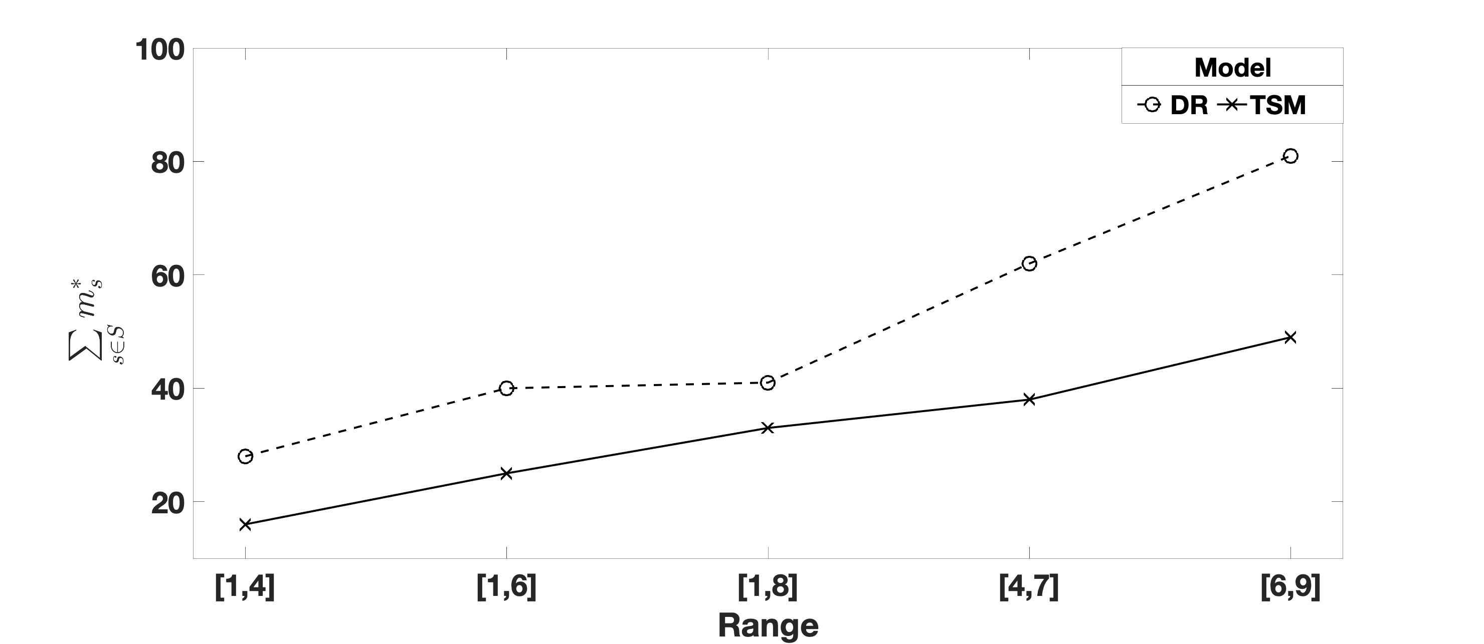
(a) Optimal fleet size vs. Demand range

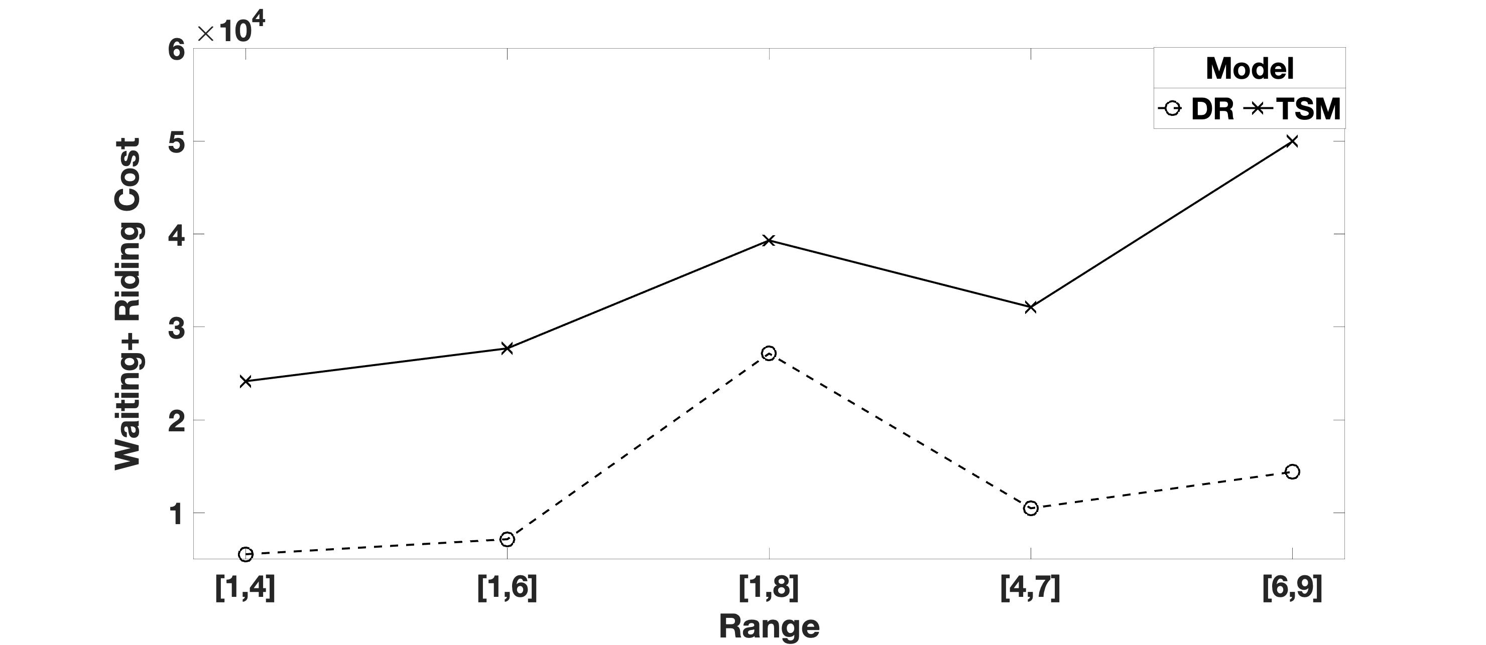
(b) Average 2nd-stage cost vs. Demand range

Figure 1: Optimal fleet size ($\sum\limits_{s\in S}m_{s}^{*}$) and the associated second-stage cost (waiting+riding time costs) under different demand range. TSM is the two-stage SP model

Impact of cost parameters

Next, we analyze the DR and SP solutions’ sensitivity to the cost parameters. We fix the demand range to [1,4] and [4,7] as examples of a low and relatively high volume of passengers, and vary $f_{s}\in\{4,000,7,000,10,000\}$ and $(\beta_{w},\beta_{r})\in\{(1,2),(8,4),(32,16)\}$. Figures 2 and 3 present the optimal fleet size, $\sum\limits_{s\in S}m_{s}^{*}$, and the associated second-stage (waiting+riding time costs) cost as a function of $f_{s}$ and $(\beta_{w},\beta_{r})$ under demand range $[1,4]$ and $[1,7]$, respectively.

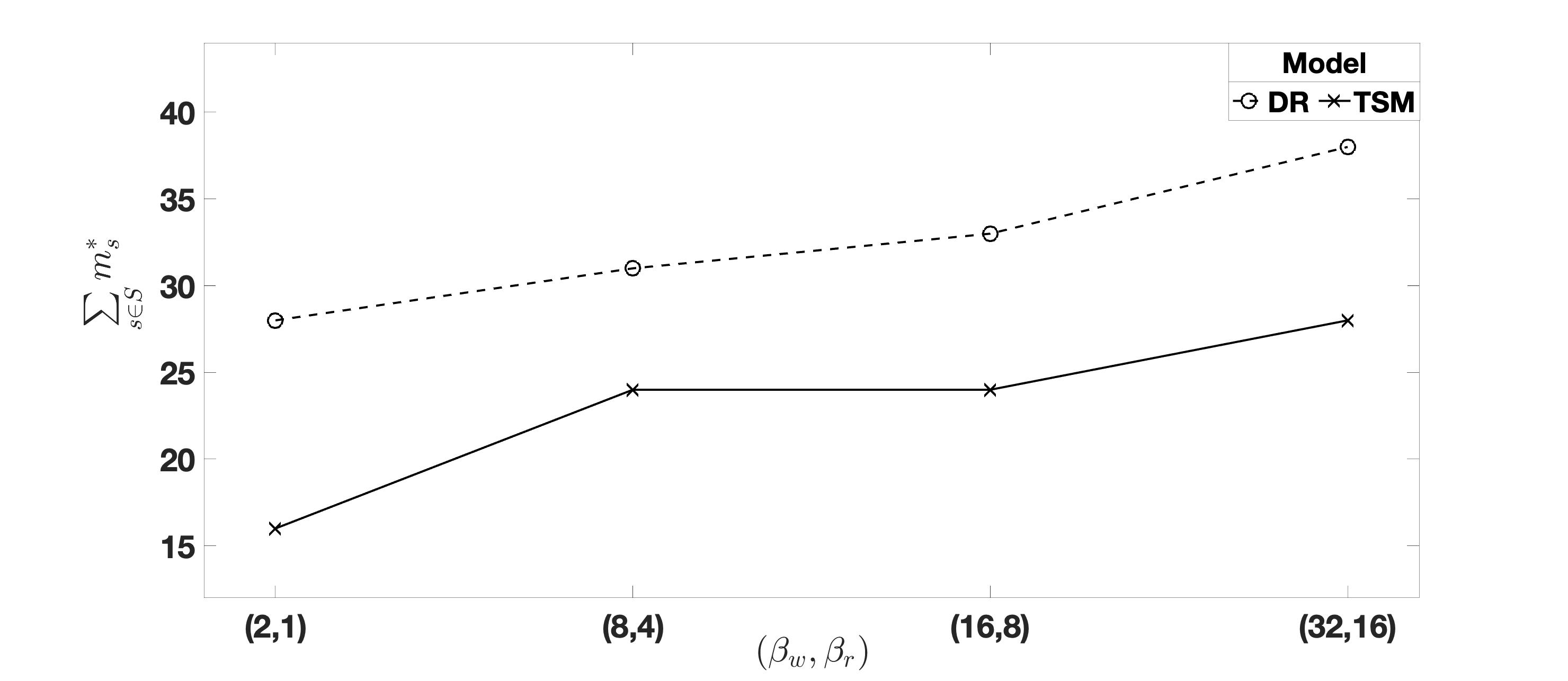
(a) Optimal fleet size vs. ($\beta_{w},\beta_{r}$), $f_{s}=4,000$

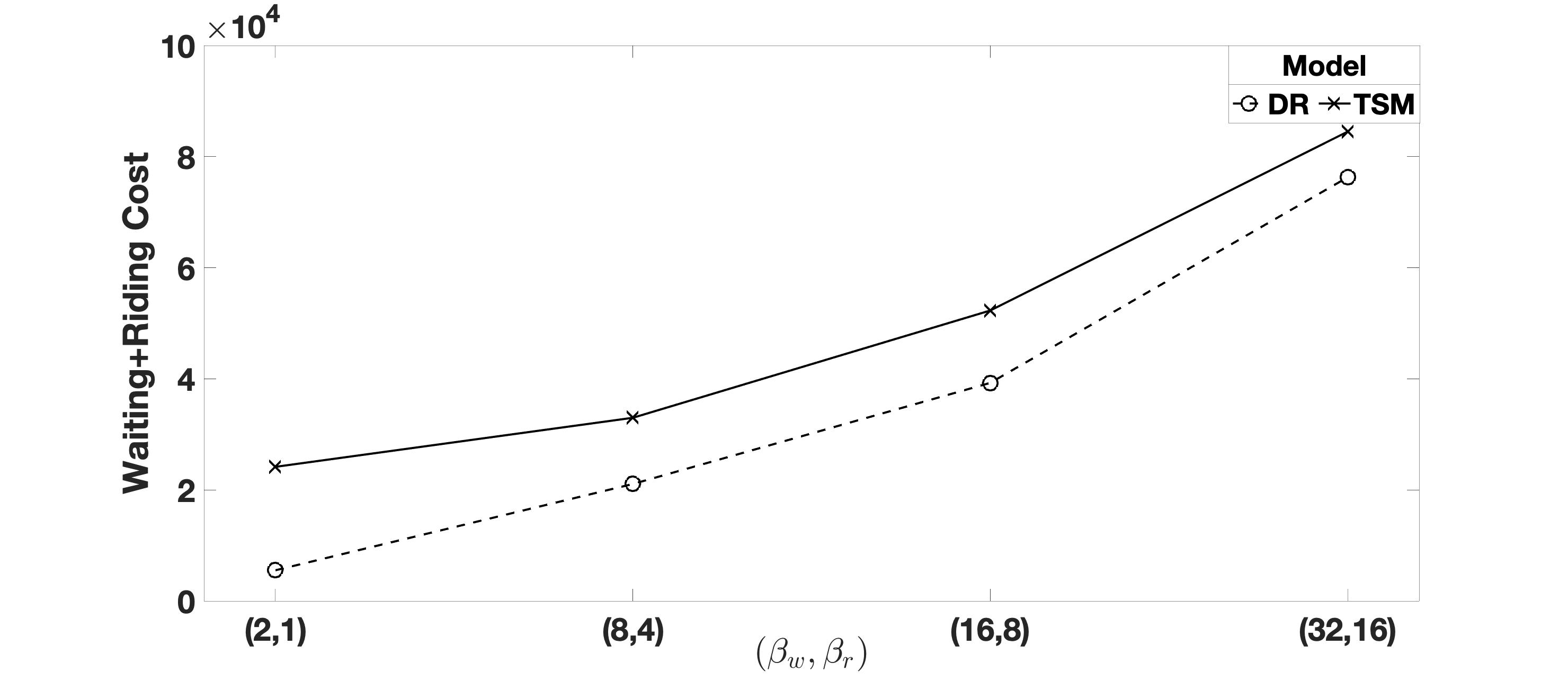
(b) Average 2nd-stage cost vs. ($\beta_{w},\beta_{r}$), $f_{s}=4,000$

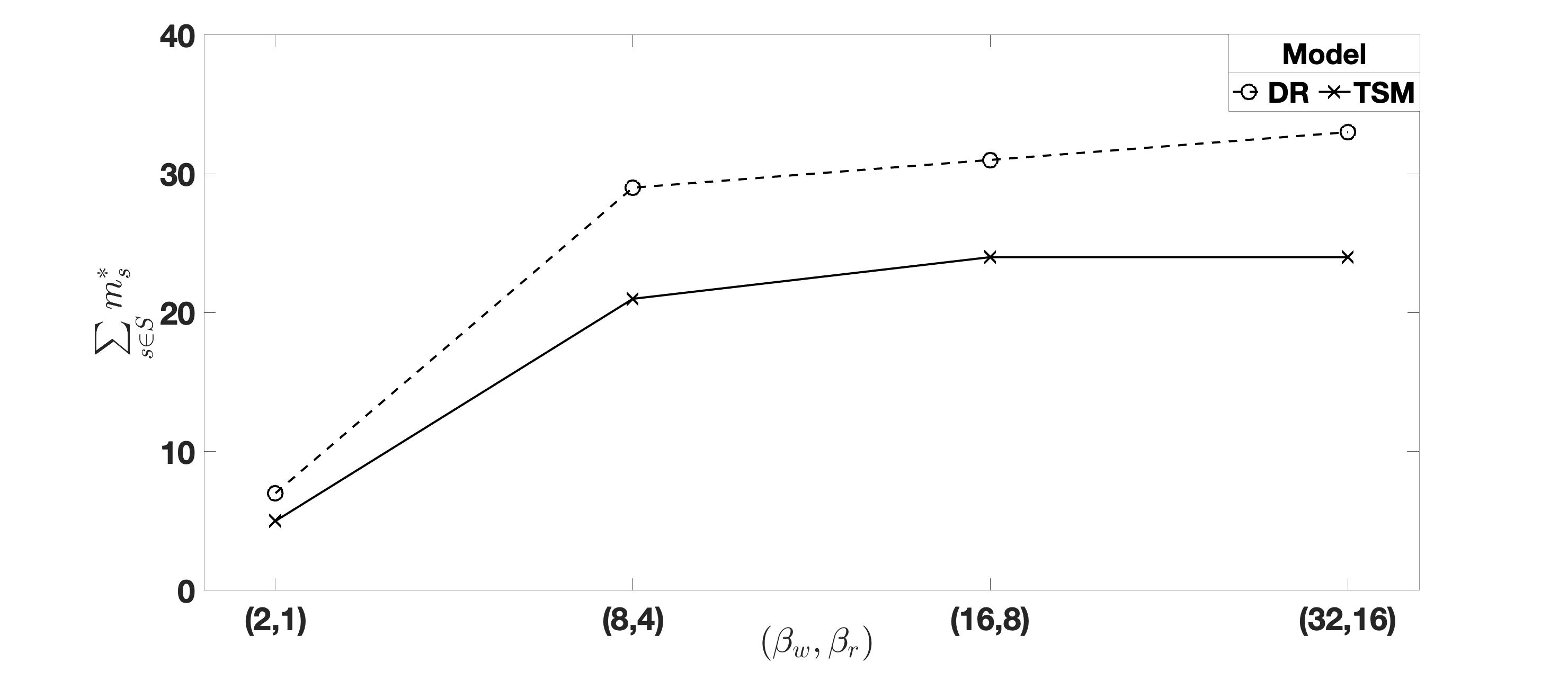
(c) Optimal fleet size vs. ($\beta_{w},\beta_{r}$), $f_{s}=7,000$

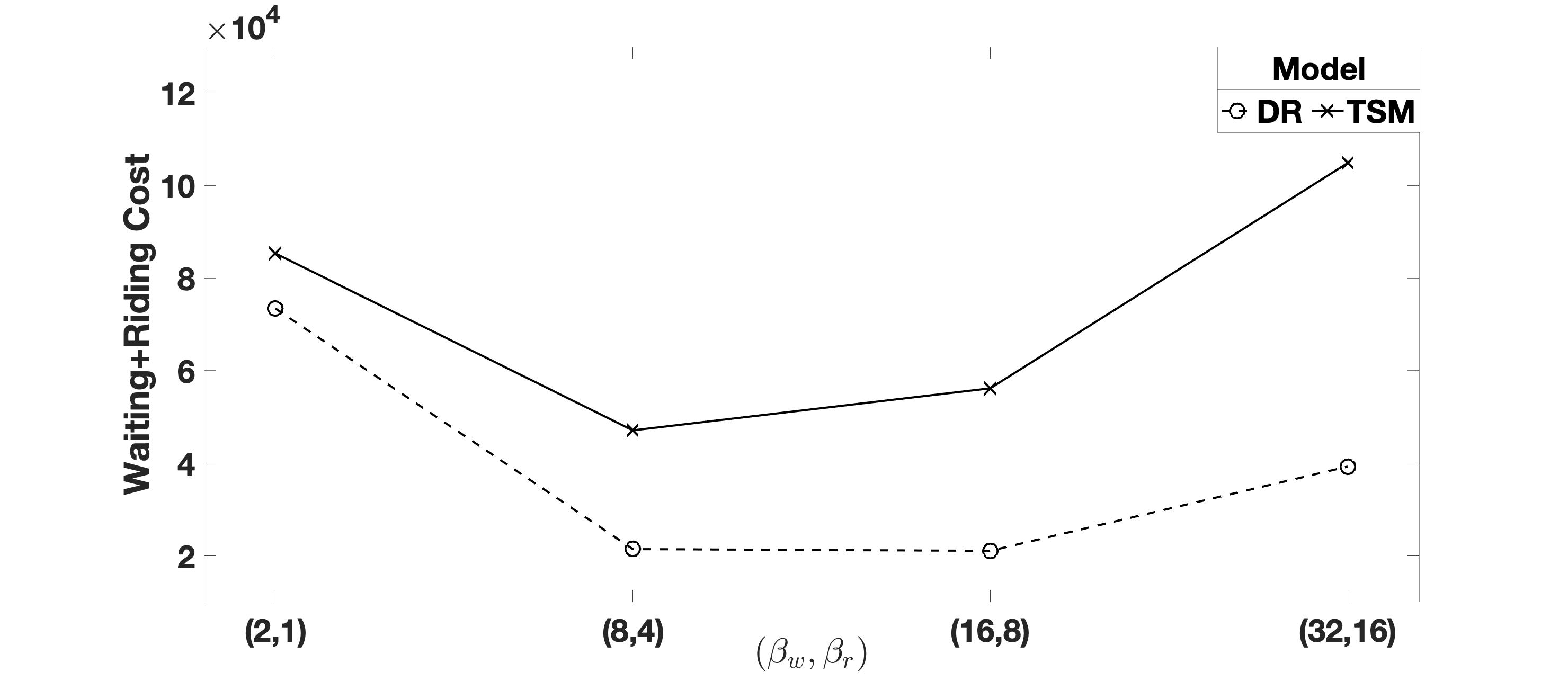
(d) Average 2nd-stage cost vs. ($\beta_{w},\beta_{r}$), $f_{s}=7,000$

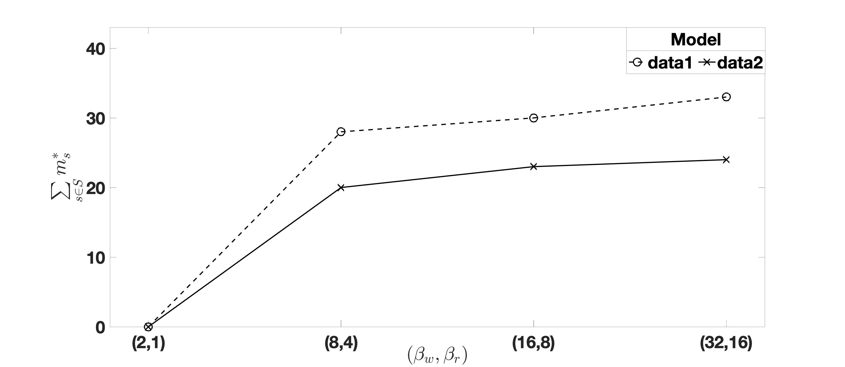
(e) Optimal fleet size vs. ($\beta_{w},\beta_{r}$), $f_{s}=10,000$

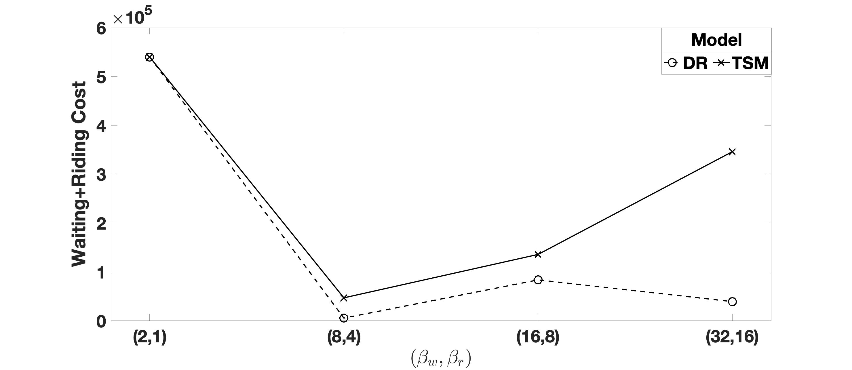
(f) Average 2nd-stage cost vs. ($\beta_{w},\beta_{r}$), $f_{s}=10,000$

Figure 2: Optimal fleet size ($\sum\limits_{s\in S}m_{s}^{*}$) and the associated second-stage cost (waiting+riding time costs) under demand range $[1,4]$ and different values of $f_{s}$ and ($\beta_{w},\beta_{r}$). TSM is the two-stage SP model.

We first observe that the optimal fleet size, $\sum\limits_{s\in S}m_{s}^{*}$ , yielded by the DR model is always larger than that of the SP model under all values of $f_{s}$ and ($\beta_{w},\beta_{r}$). Second, we observe that both models allocate more vehicles under [4,7] than under [1,4], irrespective of the values of cost parameters, which makes sense given that the former implies a higher volume of demand for last-mile service that needs fulfilling. Third, we observe that for a fixed value of ($\beta_{w},\beta_{r}$), the optimal fleet size $\sum\limits_{s\in S}m_{s}^{*}$ of the DR and SP decreases as the unit fixed cost $f_{s}$ increases. For example, when ($\beta_{w},\beta_{r}$)= (2,1) and range equal [4,7], the $\sum\limits_{s\in S}m_{s}^{*}$ of the DR and SP, respectively, decreases from 62 and 39 to 12 and 7 vehicles as $f_{s}$ increases from $f_{s}=4,000$ to $f_{s}=7,000$ (see Figure 3(a) and 3(c)).

Fourth, we observe that as the values of ($\beta_{w},\beta_{r}$) increase (i.e., passenger waiting and riding time become more important/expensive), the optimal fleet size $\sum\limits_{s\in S}m_{s}^{*}$ yielded by DR and SP increase regardless of the unit fixed cost $f_{s}$ and range of passengers. Finally, we observe that by allocating a larger fleet, the DR always yields a substantially lower second-stage cost (i.e., waiting and riding times) than the SP, which indicates a better quality of service for passengers. However, this of course comes at a higher fixed cost. The relative difference in the fixed cost between DR and SP ranges from 0 to 40%, and the relative difference in the second-stage cost ($\frac{DR-{\color[rgb]{0,0,0}SP}}{DR}\times 100\%$) from 15% to 333%. Practitioners may be willing to pay the extra one-time fixed cost of DR solutions to provide a better quality of service in terms of lower waiting and riding times, and thus maintain customer satisfaction and a good business reputation.

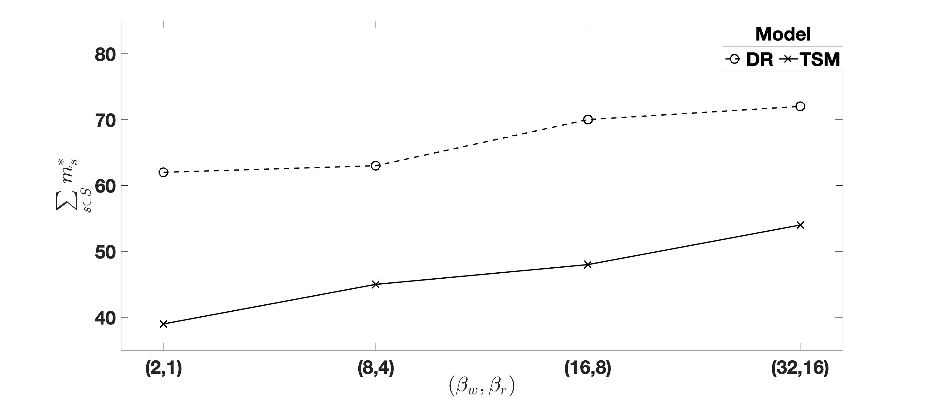
(a) Optimal fleet size vs. ($\beta_{w},\beta_{r}$), $f_{s}=4,000$

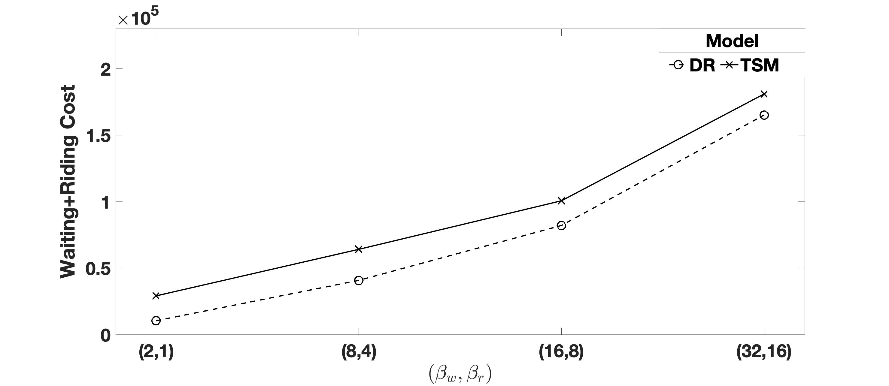
(b) Average 2nd-stage cost vs. ($\beta_{w},\beta_{r}$), $f_{s}=4,000$

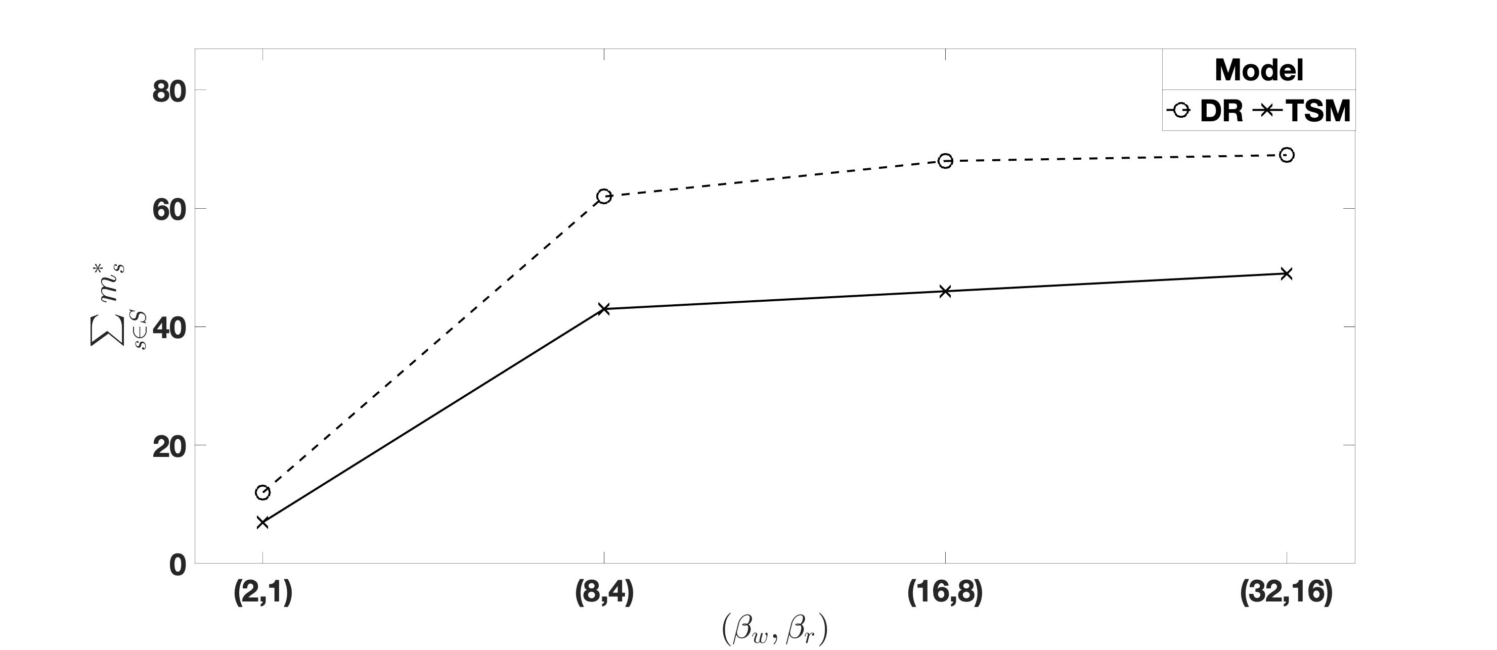
(c) Optimal fleet size vs. ($\beta_{w},\beta_{r}$), $f_{s}=7,000$

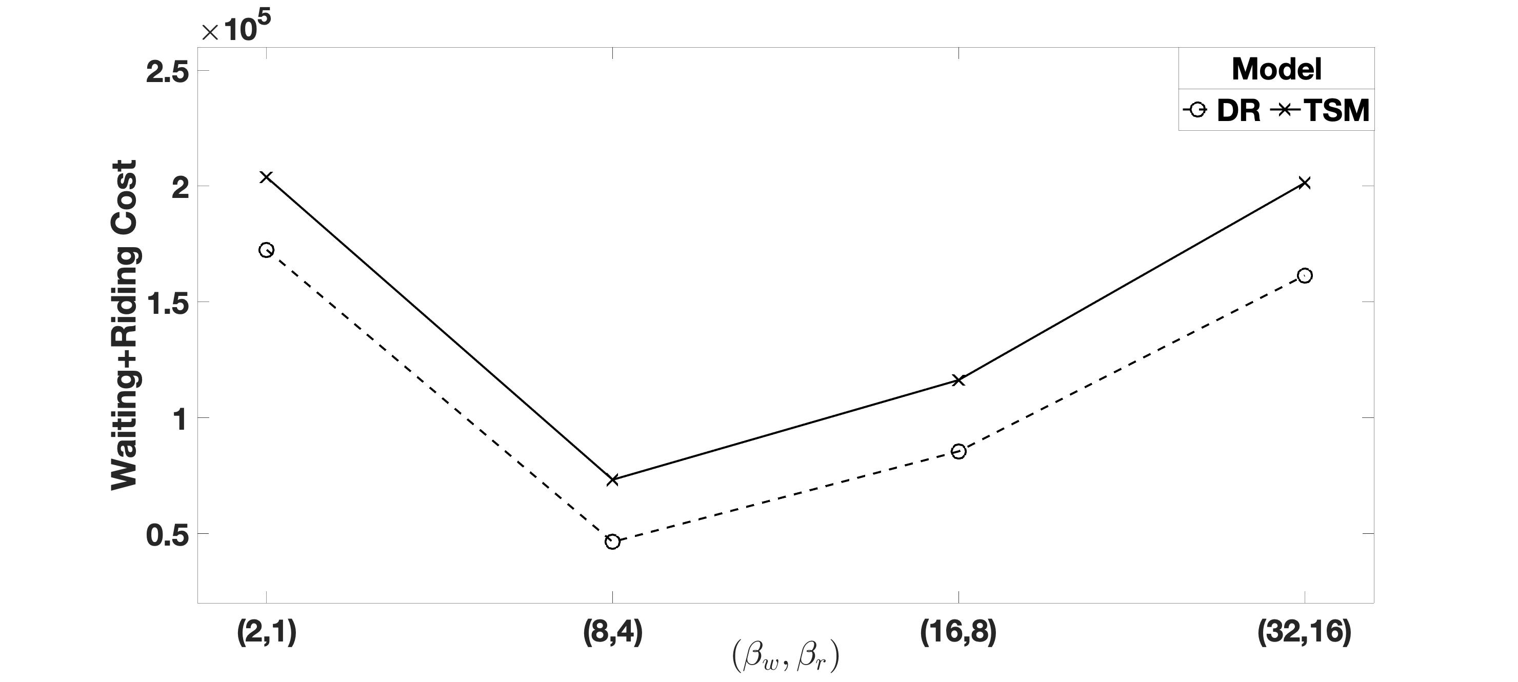
(d) Average 2nd-stage cost vs. ($\beta_{w},\beta_{r}$), $f_{s}=7,000$

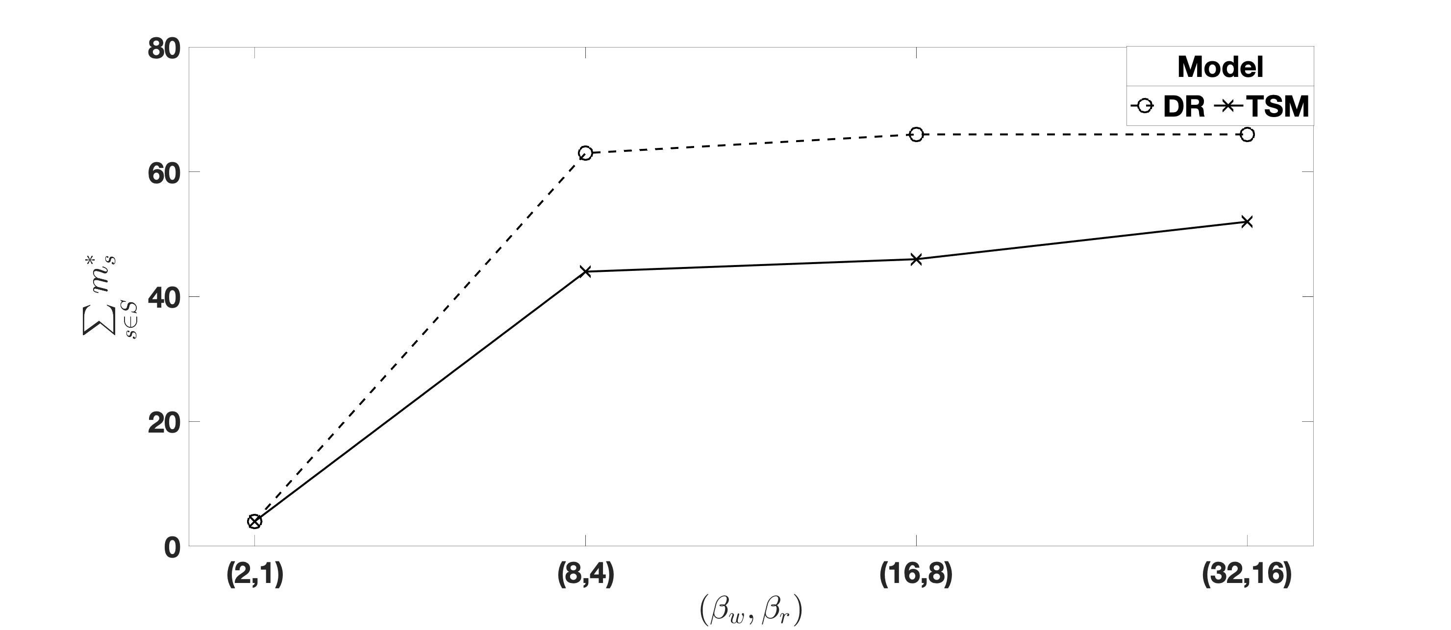
(e) Optimal fleet size vs. ($\beta_{w},\beta_{r}$), $f_{s}=10,000$

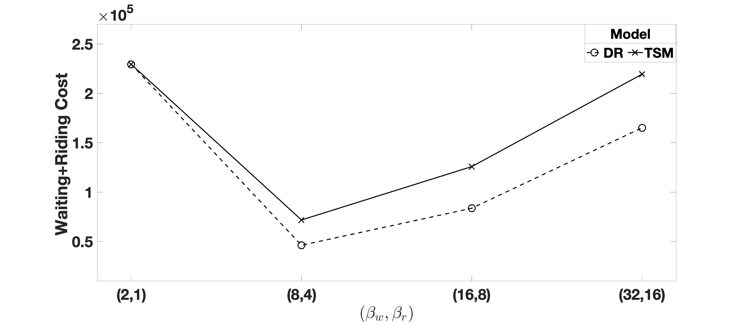
(f) Average 2nd-stage cost vs. ($\beta_{w},\beta_{r}$), $f_{s}=10,000$

Figure 3: Optimal fleet size ($\sum\limits_{s\in S}m_{s}^{*}$) and the associated second-stage cost (waiting+riding time costs) under demand range $[4,7]$ and different values of $f_{s}$ and ($\beta_{w},\beta_{r}$). TSM is the two-stage SP model.

5 Conclusion

In this paper, we investigate the fleet sizing and allocation problem for the on-demand last-mile transportation systems. Specifically, we consider the perspective of a last-mile service provider who wants to determine the number of servicing vehicles allocated to multiple service regions. In each service region, passengers demanding last-mile services arrive in batches, and allocated vehicles deliver passengers to their final destinations. The size of each batch of passengers is random and hard to predict in advance. The quality of fleet-allocation decisions is a function of vehicle fixed cost plus a weighted sum of passenger’s waiting time before boarding a vehicle and in-vehicle riding time.

We propose, analyze, and evaluate the computational and operational performance of two models for the fleet sizing and allocation problem, assuming known and unknown distribution of the demand, respectively. First, we propose a stochastic programming model to minimize the the fixed cost of allocated vehicles and the expectation of a weighted sum of passenger waiting and riding times, under a distributional belief of demand. Second, we propose a distributionally robust model to minimize the fixed cost of vehicles and the worst-case (i.e., maximum) expectation of passenger waiting time and riding times. We also conduct a set of numerical experiments and discuss the insights and implications by examining trade-offs between total cost, fleet size, and passenger waiting and riding times.

Our study opens other avenues that merit further exploration. To name a few, (1) LMTS fleet sizing and allocation given train arrival uncertainty; (2) LMTS planning and operations under certain special types of demand uncertainty; e.g., multi-modal distribution of demand; (3) fleet sizing and allocation for an on-demand transportation system that combines last- and first-mile services; (4) pricing for last-mile services for multiple service regions with demand uncertainty; (5) incentive and subsidy mechanism design if drivers in the fleet are independent income-seeking decision-makers (e.g., Sun et al. (2019), Zhu et al. (2021)); and (6) distributionally robust optimization models for other optimization problems in on-demand transportation; e.g., vehicle allocation, routing, and scheduling for hybrid services with both fixed and flexible routes. Finally, our computational experiment is not all based on real-world case studies or exact data due to the lack of benchmark instances on the specific LMTS problem that we address in this paper. We hope that our approach and results will also motivate future data collection efforts and standardized benchmark instances. The availability of high-quality data will enable the development of data-driven approaches for this and other emerging LMTS problems.

Acknowledgment

We want to thank all of our colleagues and practitioners who have contributed significantly to the related literature. We are grateful to the anonymous reviewers for their insightful comments and suggestions that allowed us to improve the paper. Dr. Karmel S. Shehadeh dedicates her effort in this paper to every little dreamer in the whole world who has a dream so big and so exciting. Believe in your dreams and do whatever it takes to achieve them–the best is yet to come for you.

References

Appendix A Proof of Proposition 3

Proof.

$$\max_{\boldsymbol{n}\in[\boldsymbol{\underline{n},\overline{n}}]} \Big{\{}\sum\limits_{s\in S}\sum\limits_{i\in I_{s}}\sum\limits_{j\in J_{s}}n_{i,j,s}(\Gamma_{i,j,s}-\rho_{i,j,s})+\sum\limits_{s\in S}\sum\limits_{i\in I_{s}}\sum\limits_{k\in K_{s}}cw_{i,k,s}\psi_{i,k,s}\Big{\}}$$ (21a)

s.t. $$\ \ \Gamma_{i,j,s}-\Gamma_{i+1,j,s}\leq\beta^{\mbox{\tiny w}}h,\qquad\forall(s,i,j)$$ (21b)

$$\ \ \phi_{j,k}(\Gamma_{i,j,s}+\psi_{i,k,s})\leq t_{j,k}\beta^{\mbox{\tiny r}},\qquad\forall(i,j,k,s)$$ (21c)

$$\ \ \psi_{i,k,s}\leq 0,\ \Gamma_{i,j,s}\geq 0,\ \Gamma_{I+1,j,s}=0,\qquad\forall(i,j,k,s)$$ (21d)

First, we rewrite constraints (21c) as $\phi_{j,k}\psi_{i,k,s}\leq t_{j,k}\beta^{\mbox{\tiny r}}-\phi_{j,k}\Gamma_{i,j,s}$. Given that $\psi_{i,k,s}\leq 0$ and the objective of maximizing a positive number times $\Gamma_{i,j,s}$ in (21), then, without loss of optimality, we can assume that $\Gamma_{i,j,s}\geq 0$, for all $i\in[I],\ j\in[J],$ and $s\in[S]$. Note that if $\Gamma_{i,j,s}<0$, then $\phi_{j,k}\psi_{i,k,s}\leq t_{j,k}\beta^{\mbox{\tiny r}}+\phi_{j,k}|\Gamma_{i,j,s}|=$ a positive number. Given that $\psi_{i,k,s}\leq 0$, then in this case, condition $\phi_{j,k}\psi_{i,k,s}\leq$ a positive number is relaxed and the first term in the objective will be negative for $\Gamma_{i,j,s}$. It follows that $\Gamma_{i,j,s}\geq 0$ in the optimal solution. Second, we consider the following cases, for fixed $s\in S,i\in I_{s},j\in J_{s}$ and fixed $\rho_{i,j,s}$:

• Case 1: when $\rho_{i,j,s}\geq 0$

  • If $0\leq\Gamma_{i,j,s}<\rho_{i,j,s}$. In this case, $(\Gamma_{i,j,s}-\rho_{i,j,s})<0$ and so $n_{i,j,s}=\underline{n}_{i,j,s}$ maximizes (21a). Thus, the first term in the objective function (21a) reduces to:

    $$\underline{n}_{i,j,s}(\Gamma_{i,j,s}-\rho_{i,j,s})\leq 0$$ (22)

  • If $\Gamma_{i,j,s}>\rho_{i,j,s}\geq 0$. In this case, $(\Gamma_{i,j,s}-\rho_{i,j,s})>0$, $n_{i,j,s}=\overline{n}_{i,j,s}$, and the first term in the objective function (21a) reduces to:

    $$\overline{n}_{i,j,s}(\Gamma_{i,j,s}-\rho_{i,j,s})\geq 0$$ (23)

  Note that (23)$>$(22). It follows that if $\rho_{i,j,s}\geq 0$, then $\Gamma_{i,j,s}\geq\rho_{i,j,s}$ and $n_{i,j,s}=\overline{n}_{i,j,s}$ maximizes the objective of (21). In other words, when $\rho_{i,j,s}\geq 0$, $n_{i,j,s}=\overline{n}_{i,j,s}$ is optimal to (21) and the objective equals $\overline{n}_{i,j,s}(\Gamma_{i,j,s}-\rho_{i,j,s})$ as in (23).

• Case 2: when $\rho_{i,j,s}<0$, then $\Gamma_{i,j,s}>\rho_{i,j,s}$ (given that $\Gamma_{i,j,s}\geq 0$). In this case, $(\Gamma_{i,j,s}-\rho_{i,j,s})=(\Gamma_{i,j,s}+|\rho_{i,j,s}|)\geq 0$, $n_{i,j,s}=\overline{n}_{i,j,s}$, and the first term in the objective (21a) reduces to:

  $$\overline{n}_{i,j,s}(\Gamma_{i,j,s}+|\rho_{i,j,s}|)\geq 0$$ (24)

  Thus, when $\rho_{i,j,s}<0$, the objective of (21) equals to $\overline{n}_{i,j,s}(\Gamma_{i,j,s}-\rho_{i,j,s})$

It follows from the above analysis, that $n_{i,j,s}=\overline{n}_{i,j,s}$ is optimal to (21). Thus,, w.l.o.o., we can set $n_{i,j,s}=\overline{n}_{i,j,s}$ in (21). Accordingly, (21) is equivalent to

$$\max\limits_{\Gamma,\psi} \ \ \Big{\{}\sum\limits_{s\in S}\sum\limits_{i\in I_{s}}\sum\limits_{j\in J_{s}}\overline{n}_{i,j,s}(\Gamma_{i,j,s}-\rho_{i,j,s})+\sum\limits_{s\in S}\sum\limits_{i\in I_{s}}\sum\limits_{k\in K_{s}}cw_{i,k,s}\psi_{i,k,s}\Big{\}}$$ (25a)

s.t. $$\ \ \Gamma_{i,j,s}-\Gamma_{i+1,j,s}\leq\beta^{\mbox{\tiny w}}h,\qquad\forall(s,i,j)$$ (25b)

$$\ \ \phi_{j,k}(\Gamma_{i,j,s}+\psi_{i,k,s})\leq t_{j,k}\beta^{\mbox{\tiny r}},\qquad\forall(i,j,k,s)$$ (25c)

$$\ \ \psi_{i,k,s}\leq 0,\ \Gamma_{I+1,j,s}=0,\qquad\forall(i,j,k,s)$$ (25d)

For fixed $w$ and $\rho$, problem (25) is a bounded and feasible linear program. We formulate (25) in its dual form as

$$\min\limits_{y\geq 0,x\geq 0} \ \sum\limits_{s\in S}\sum\limits_{i\in I_{s}}\sum\limits_{j\in J_{s}}\Big{[}\beta^{\mbox{\tiny w}}hy_{i,j,s}+\sum\limits_{k\in K_{s}}t_{j,k}\beta^{\mbox{\tiny r}}x_{i,j,k,s}\Big{]}-\sum\limits_{s\in S}\sum\limits_{i\in I_{s}}\sum\limits_{j\in J_{s}}\overline{n}_{i,j,s}\rho_{i,j,s}$$ (26a)

s.t. $$\ y_{0,j,s}+\sum\limits_{k\in K_{s}}\phi_{j,k}x_{0,j,k,s}\geq\overline{n}_{0,j,s},\qquad\forall s\in S,\ j\in J_{s}$$ (26b)

$$\ y_{i,j,s}-y_{i-1,j,s}+\sum\limits_{k\in K_{s}}\phi_{j,k}x_{i,j,k,s}\geq\overline{n}_{i,j,s},\qquad\forall s\in S,\ i\in I_{s}\setminus\{0\},\ j\in J_{s}$$ (26c)

$$\ \sum\limits_{j\in J_{s}}\phi_{j,k}x_{i,j,k,s}\leq cw_{i,k,s},\qquad\forall s\in S,\ i\in I_{s},\ j\in J_{s}$$ (26d)

Combining the inner problem in the form of (26) with the outer minimization problems in (14) and (12), we derive the following equivalent reformulation of the DR model in (12)

$$\min \Bigg{\{}\sum_{s\in S}f_{s}m_{s}+\sum\limits_{s\in S}\sum\limits_{i\in I_{s}}\sum\limits_{j\in J_{s}}(\mu_{i,j,s}-\overline{n}_{i,j,s})\rho_{i,j,s}+\sum\limits_{s\in S}\sum\limits_{i\in I_{s}}\sum\limits_{j\in J_{s}}\Big{[}\beta^{\mbox{\tiny w}}hy_{i,j,s}+\sum\limits_{k\in K_{s}}t_{j,k}\beta^{\mbox{\tiny r}}x_{i,j,k,s}\Big{]}\Bigg{\}}$$ (27a)

s.t. $$\ y_{0,j,s}+\sum\limits_{k\in K_{s}}\phi_{j,k}x_{0,j,k,s}\geq\overline{n}_{0,j,s},\qquad\forall s\in S,\ j\in J_{s}$$ (27b)

$$\ y_{i,j,s}-y_{i-1,j,s}+\sum\limits_{k\in K_{s}}\phi_{j,k}x_{i,j,k,s}\geq\overline{n}_{i,j,s},\qquad\forall s\in S,\ i\in I_{s}\setminus\{0\},\ j\in J_{s}$$ (27c)

$$\ \sum\limits_{j\in J_{s}}\phi_{j,k}x_{i,j,k,s}\leq cw_{i,k,s},\qquad\forall s\in S,\ i\in I_{s},\ j\in J_{s}$$ (27d)

$$\ m\in\mathcal{M},\ w\in\mathcal{W},\ y\geq 0,\ x\geq 0,\ \rho\geq 0$$ (27e)

∎

Appendix B Sample average approximation of SP

There are two well-known difficulties in obtaining an (exact) optimal solution to the SP in (8). First, evaluating the value of $\mathbb{E}_{\mathbb{P}}[Q(m,\xi)]$ involves taking multi-dimensional integrals and solving a huge number of similar integer programs. Second, both $\mathbb{E}_{\mathbb{P}}[Q(x,\xi)]$ and $Q(x,\xi)$ are non-convex and discontinuous (Birge and Louveaux, 2011; Shapiro et al., 2009). In view of these two difficulties, we resort to approximation solution approaches, and the sample average approximation (SAA) approach in particular.

In SAA, we replace the distribution of $\xi$ with a (discrete) empirical distribution based on $R$ independent and identically distributed (i.i.d.) samples of random demand, then solve the sample average approximation (28) of (8). Note that in the SAA formulations (28), we associate all scenario-dependent parameters, variables, and constraints with a scenario index $r$ for all $r=1,\ldots,R$. For example, parameters $n$ by $n^{\mbox{\tiny r}}$ to represent number of passengers realized in scenario $r$, and variables $u$ are replaced by $u^{r}$ to represent the number of unserved passengers in scenario $r$. In addition, constraints (7b)–(7e) are incorporated in each scenario.

$$v_{R}=\min\hat{f}_{R}:=\frac{1}{R}\sum\limits_{r=1}^{R}\Big{[}\ \beta^{\mbox{\tiny w}}\sum\limits_{s\in S}\sum\limits_{i\in I_{s}}\sum\limits_{j\in J_{s}}hu_{i,j,s}^{r}+\beta^{\mbox{\tiny r}}\sum\limits_{s\in S}\sum\limits_{i\in I_{s}}\sum\limits_{j\in J_{s}}\sum\limits_{k\in K_{s}}t_{j,k}z_{i,j,k,s}^{r}\Big{]}$$ (28a)

$$\ \ \text{s.t.}\ \ \ \ m\in\mathcal{M},\ w\in\mathcal{W}$$ (28b)

$$\quad\ \quad\quad\eqref{Const1}-\eqref{Const6},\ \ \text{for }r=1,\ldots,R$$ (28c)

Appendix C Construction and Statistics of the NYC Instance

We construct the NYC instance based on the dataset the procedure as follows:

1. Select 4 metro stations that are relatively far away from each other in Manhattan, NYC;

2. For each station, construct a 1-mile by 1-mile square as a last-mile service region with the station located in the center;

3. For each service region, consider the passengers with destination within the region as potential demand for LMTS;

4. For each service region $s$, cluster the passenger destinations to $J_{s}$ clusters; assume the center of each cluster $j_{s}$ as the location of a last-mile stop $j_{s}$ to cover all passengers in that cluster;

5. For each last-mile stop $j$ in service region $s$, record the number of passengers going to that stop (i.e., with destination in that cluster) within each time interval $i$ (e.g., every 5 or 10 minutes) as the batch demand $n_{i,j,s}$ for the LMTS;

6. For each last-mile stop $j$ in service region $s$, compute the upper bound, lower bound, $20\%$ percentile, and $80\%$ percentile for batch demand $n_{i,j,s}$ across $i$ in certain period (e.g., 10 am to 11 am);

7. Using the locations of all last-mile stops in each service region $s$, generate $K_{s}$ routes to serve a subset of stops (e.g., serve 1, 2, and 3 stops), all of which start from and return to the metro station;

8. For each route $k$, record its total travel time $t_{k}$, stop-route configuration $\phi_{j,k}$, and travel time to each stop $t_{j,k}$.

Table 1: NYC Instance.
Notation: $S$ is number of regions, $s$ is a region, $J_{s}$ is number of last-mile stops in regions $s$, $K_{s}$ is number of routes in region $s$.

Inst	$S$	$s$	$J_{s}$	$K_{s}$
NYC	4	$\ \ s=1$	5	31
		$\ \ s=2$	6	30
		$\ \ s=3$	4	15
		$\ \ s=4$	5	20

Table 2: Statistics of the batch demand for each last-mile stop per service region in the NYC instance.
Notation:$\mu$ and $\sigma$ are respectively the empirical mean and standard deviations of batch demand $n_{i,j,s}$.

Region, $s$	LM stop, $j$	$\mu$	$\sigma$
$s=1$	$j=1$	1.11	1.64
	$j=2$	1.13	1.88
	$j=3$	2.23	2.72
	$j=4$	1.13	2.45
	$j=5$	1.30	2.25
$s=2$	$j=1$	1.40	1.72
	$j=2$	1.43	1.93
	$j=3$	1.20	1.92
	$j=4$	2.63	2.54
	$j=5$	2.63	2.54
	$j=6$	1.83	1.89
$s=3$	$j=1$	2.43	2.86
	$j=2$	3.33	2.37
	$j=3$	2.63	3.10
	$j=4$	3.23	3.58
$s=4$	$j=1$	1.37	2.86
	$j=2$	1.13	2.37
	$j=3$	1.90	3.10
	$j=4$	1.20	3.58
	$j=5$	1.70	2.58

Appendix D Values of parameters $f_{s}$, $\beta^{w}$, and $\beta^{r}$

Let the average after-tax hourly wage of passengers be $g$/hour. According to Gomez-Ibanez et al. (1999):

• Monetary value of riding time ($76\%$ of after-tax wage): $\$0.76g$/hour$\approx\$0.0127g$/minute.

• Monetary value of waiting time ($195\%$ of after-tax wage): $\$1.95g$/hour=$\$0.0325g$/minute.

• Average hourly total fixed cost of a vehicle (with capacity 5), including the cost to rent the vehicle, wage paid to the driver, fuel cost, and other maintenance and operating costs: $b$/hour.

In the LMTS, we have $I$ trains with headway $h$ minute. The duration of the time that vehicles are needed is slightly longer than $Ih$. Then, we can approximate the fixed cost $f_{s}$, parameter $\beta^{w}$, and $\beta^{r}$ as $f_{s}=b\cdot\frac{Ih}{60}=\frac{bIh}{60}$; $\beta^{r}=0.0127g$; $\beta^{w}=0.0325g$.

Scenario 1: Assuming there is an existing fleet with no additional cost, we have $f_{s}=0$, $\beta^{r}=0.0127g$, and $\beta^{w}=0.0325g$. In the numerical experiments, we normalize $\beta^{r}$ to 1 and evaluate this scenario with the following parameters: $f_{s}=0$, $\beta^{r}=1$; $\beta^{w}\in[2,3]$.

Scenario 2: Assuming the average after-tax hourly wage of passengers (e.g., working adults who are more sensitive to riding and waiting times) $g=\$10$/hour and the average hourly total cost of a vehicle (e.g., regular vehicle) $b=\$30$/hour, then: $f_{s}=\frac{30\cdot 10\cdot 10}{60}=50$; $\beta^{r}=0.127$; $\beta^{w}=0.325$. In the numerical experiments, we normalize $\beta^{r}$ to 1 and evaluate this scenario with the following parameters: $f_{s}\in[200,600]$, $\beta^{r}=1$; $\beta^{w}\in[2,3]$.

Scenario 3: Assuming the equivalent average after-tax hourly wage of passengers (e.g., children, students, seniors, and the disabled, who are less sensitive to riding and waiting times) $g=\$3$/hour and the average hourly total cost of a vehicle (e.g., vehicle with special equipment for children, seniors, and the disables) $b=\$90$/hour, then $f_{s}=\frac{90\cdot 10\cdot 10}{60}=150$; $\beta^{r}=0.0381$; $\beta^{w}=0.0975$. In the numerical experiments, we normalize $\beta^{r}$ to 1 and evaluate this scenario with the following parameters: $f_{s}\in[2,000,6,000]$, $\beta^{r}=1$; $\beta^{w}\in[2,3]$.

Appendix E Example of In-sample performance under $f_{s}=0$

Under $f_{s}=0$, both models allocate the same numbers of vehicles. As such, they have similar in-sample and out-of-sample simulation performances for all three instances. As an example, in Table  1, we present in-sample simulation results (i.e., under set 1; perfect information) for instance 1.

Table 1: In-sample performance of optimal allocation decisions under perfect distributional information, $f_{s}=0$. The performance of two models are almost the same if demands follow the perfect (in-sample) distribution.

Instance	R	Metric	Model	TC	2nd-Stage
1	[1,4]	Mean	DR	4,590	4,590
			SP	4,572	4,572
		Median	DR	4,592	4,592
			SP	4,573	4,573
		75%-q	DR	4,722	4,722
			SP	4,750	4,750
		95%-q	DR	4,921	4,921
			SP	5,001	5,001
	[3,7]	Mean	DR	9,370	9,370
			SP	9,618	9,618
		Median	DR	9,332	9,332
			SP	9,605	9,605
		75%-q	DR	9,776	9,776
			SP	9,941	9,941
		95%-q	DR	10,403	10,403
			SP	10,509	10,509

References

- Agussurja et al. (2019) Agussurja, L., Cheng, S.-F., Lau, H. C., 2019. A state aggregation approach for stochastic multiperiod last-mile ride-sharing problems. Transportation Science 53 (1), 148–166.
- Anderson (1998) Anderson, J. E., 1998. Control of personal rapid transit systems. Journal of advanced transportation 32 (1), 57–74.
- Ben-Tal et al. (2015) Ben-Tal, A., Den Hertog, D., Vial, J.-P., 2015. Deriving robust counterparts of nonlinear uncertain inequalities. Mathematical programming 149 (1-2), 265–299.
- Berger et al. (2011) Berger, T., Sallez, Y., Raileanu, S., Tahon, C., Trentesaux, D., Borangiu, T., 2011. Personal rapid transit in an open-control framework. Computers & Industrial Engineering 61 (2), 300–312.
- Bertsimas and Popescu (2005) Bertsimas, D., Popescu, I., 2005. Optimal inequalities in probability theory: A convex optimization approach. SIAM Journal on Optimization 15 (3), 780–804.
- Bertsimas and Sim (2004) Bertsimas, D., Sim, M., 2004. The price of robustness. Operations research 52 (1), 35–53.
- Birge and Louveaux (2011) Birge, J. R., Louveaux, F., 2011. Introduction to stochastic programming. Springer Science & Business Media.
- Bly and Teychenne (2005) Bly, P., Teychenne, P., 2005. Three financial and socio-economic assessments of a personal rapid transit system. In: Automated People Movers 2005: Moving to Mainstream. pp. 1–16.
- Chen et al. (2020a) Chen, S., Wang, H., Meng, Q., 2020a. Solving the first-mile ridesharing problem using autonomous vehicles. Computer-Aided Civil and Infrastructure Engineering 35 (1), 45–60.
- Chen and Wang (2018a) Chen, Y., Wang, H., 2018a. Pricing for a last-mile transportation system. Transportation Research Part B: Methodological 107, 57–69.
- Chen and Wang (2018b) Chen, Y., Wang, H., 2018b. Why are fairness concerns so important? lessons from pricing a shared last-mile transportation system. Available at SSRN: https://ssrn.com/abstract=3168324.
- Chen et al. (2020b) Chen, Z., Sim, M., Xiong, P., 2020b. Robust stochastic optimization made easy with rsome. Management Science.
- Delage and Ye (2010) Delage, E., Ye, Y., 2010. Distributionally robust optimization under moment uncertainty with application to data-driven problems. Operations research 58 (3), 595–612.
- Esfahani and Kuhn (2018) Esfahani, P. M., Kuhn, D., 2018. Data-driven distributionally robust optimization using the wasserstein metric: Performance guarantees and tractable reformulations. Mathematical Programming 171 (1-2), 115–166.
- Gomez-Ibanez et al. (1999) Gomez-Ibanez, J., Tye, W. B., Winston, C., 1999. Essays in transportation economics and policy. The Brookings Institution, Washington, DC.
-
Hao et al. (2021)
Hao, H., Wang, H., Zhang, P., 2021. U.s. household commuting dataset and
transportation fairness. (under review).
URL https://github.com/peteryz/employment-od - Homem-de Mello and Bayraksan (2014) Homem-de Mello, T., Bayraksan, G., 2014. Monte carlo sampling-based methods for stochastic optimization. Surveys in Operations Research and Management Science 19 (1), 56–85.
- Horn (2002) Horn, M., 2002. Multi-modal and demand-responsive passenger transport systems: a modelling framework with embedded control systems. Transportation Research Part A: Policy and Practice 36 (2), 167–188.
- Jiang et al. (2017) Jiang, R., Shen, S., Zhang, Y., 2017. Integer programming approaches for appointment scheduling with random no-shows and service durations. Operations Research 65 (6), 1638–1656.
- Kamath and Pakkala (2002) Kamath, K. R., Pakkala, T., 2002. A bayesian approach to a dynamic inventory model under an unknown demand distribution. Computers & Operations Research 29 (4), 403–422.
- Ke et al. (2020) Ke, J., Yang, H., Li, X., Wang, H., Ye, J., 2020. Pricing and equilibrium in on-demand ride-pooling markets. Transportation Research Part B: Methodological 139, 411–431.
- Kim et al. (2015) Kim, S., Pasupathy, R., Henderson, S. G., 2015. A guide to sample average approximation. In: Handbook of simulation optimization. Springer, pp. 207–243.
- Kleywegt et al. (2002) Kleywegt, A. J., Shapiro, A., Homem-de Mello, T., 2002. The sample average approximation method for stochastic discrete optimization. SIAM Journal on Optimization 12 (2), 479–502.
- Lees-Miller et al. (2009) Lees-Miller, J., Hammersley, J., Davenport, N., 2009. Ride sharing in personal rapid transit capacity planning. In: Automated People Movers 2009: Connecting People, Connecting Places, Connecting Modes. pp. 321–332.
- Linderoth et al. (2006) Linderoth, J., Shapiro, A., Wright, S., 2006. The empirical behavior of sampling methods for stochastic programming. Annals of Operations Research 142 (1), 215–241.
- Liu et al. (2019) Liu, L., Sun, L., Chen, Y., Ma, X., 2019. Optimizing fleet size and scheduling of feeder transit services considering the influence of bike-sharing systems. Journal of Cleaner Production 236, 117550.
- Liu et al. (2012) Liu, Z., Jia, X., Cheng, W., 2012. Solving the last mile problem: Ensure the success of public bicycle system in beijing. Procedia-Social and Behavioral Sciences 43, 73–78.
- Mak et al. (2014) Mak, H.-Y., Rong, Y., Zhang, J., 2014. Appointment scheduling with limited distributional information. Management Science 61 (2), 316–334.
- Mueller and Sgouridis (2011) Mueller, K., Sgouridis, S. P., 2011. Simulation-based analysis of personal rapid transit systems: service and energy performance assessment of the masdar city prt case. Journal of Advanced Transportation 45 (4), 252–270.
- Quadrifoglio et al. (2008) Quadrifoglio, L., Dessouky, M. M., Ordóñez, F., 2008. A simulation study of demand responsive transit system design. Transportation Research Part A: Policy and Practice 42 (4), 718–737.
- Rahimian and Mehrotra (2019) Rahimian, H., Mehrotra, S., 2019. Distributionally robust optimization: A review. arXiv preprint arXiv:1908.05659.
- Serra et al. (2019) Serra, T., Raghunathan, A. U., Bergman, D., Hooker, J., Kobori, S., 2019. Last-mile scheduling under uncertainty. In: International Conference on Integration of Constraint Programming, Artificial Intelligence, and Operations Research. Springer, pp. 519–528.
- Shapiro et al. (2009) Shapiro, A., Dentcheva, D., Ruszczyński, A., 2009. Lectures on stochastic programming: modeling and theory. SIAM.
- Shapiro et al. (2014) Shapiro, A., Dentcheva, D., Ruszczyński, A., 2014. Lectures on stochastic programming: modeling and theory. SIAM.
- Shehadeh (2021) Shehadeh, K. S., 2021. Distributionally robust optimization approaches for a stochastic mobile facility routing and scheduling problem. arXiv preprint arXiv:2009.10894.
- Shehadeh and Padman (2021) Shehadeh, K. S., Padman, R., 2021. A distributionally robust optimization approach for stochastic elective surgery scheduling with limited intensive care unit capacity. European Journal of Operational Research 290 (3), 901–913.
- Shehadeh and Sanci (2021) Shehadeh, K. S., Sanci, E., 2021. Distributionally robust facility location with bimodal random demand. Computers & Operations Research 134, 105257.
- Smith and Winkler (2006) Smith, J. E., Winkler, R. L., 2006. The optimizer’s curse: Skepticism and postdecision surprise in decision analysis. Management Science 52 (3), 311–322.
- Soyster (1973) Soyster, A. L., 1973. Convex programming with set-inclusive constraints and applications to inexact linear programming. Operations research 21 (5), 1154–1157.
- Sun et al. (2019) Sun, H., Wang, H., Wan, Z., 2019. Model and analysis of labor supply for ride-sharing platforms in the presence of sample self-selection and endogeneity. Transportation Research Part B: Methodological 125, 76–93.
- Thiele (2010) Thiele, A., 2010. A note on issues of over-conservatism in robust optimization with cost uncertainty. Optimization 59 (7), 1033–1040.
- Wang (2019) Wang, H., 2019. Routing and scheduling for a last-mile transportation system. Transportation Science 53 (1), 131–147.
- Wang and Odoni (2016) Wang, H., Odoni, A., 2016. Approximating the performance of a “last mile” transportation system. Transportation Science 50 (2), 659–675.
- Wang and Yang (2019) Wang, H., Yang, H., 2019. Ridesourcing systems: A framework and review. Transportation Research Part B: Methodological 129, 122–155.
- Xu and Meng (2019) Xu, M., Meng, Q., 2019. Fleet sizing for one-way electric carsharing services considering dynamic vehicle relocation and nonlinear charging profile. Transportation Research Part B: Methodological 128, 23–49.
- Zhang et al. (2019) Zhang, H., Sheppard, C. J., Lipman, T. E., Moura, S. J., 2019. Joint fleet sizing and charging system planning for autonomous electric vehicles. IEEE Transactions on Intelligent Transportation Systems 21 (11), 4725–4738.
- Zhu et al. (2021) Zhu, Z., Ke, J., Wang, H., 2021. A mean-field markov decision process model for spatial-temporal subsidies in ride-sourcing markets. Transportation Research Part B: Methodological 150, 540–565.
- Zhu et al. (2020) Zhu, Z., Qin, X., Ke, J., Zheng, Z., Yang, H., 2020. Analysis of multi-modal commute behavior with feeding and competing ridesplitting services. Transportation Research Part A: Policy and Practice 132, 713–727.