Abstract

In this article, we propose the outcome-adjusted balance measure to perform model selection for the generalized propensity score (GPS), which serves as an essential component in estimation of the pairwise average treatment effects (ATEs) in observational studies with more than two treatment levels. The primary goal of the balance measure is to identify the GPS model specification such that the resulting ATE estimator is consistent and efficient. Following recent empirical and theoretical evidence, we establish that the optimal GPS model should only include covariates related to the outcomes. Given a collection of candidate GPS models, the outcome-adjusted balance measure imputes all baseline covariates by matching on each candidate model, and selects the model that minimizes a weighted sum of absolute mean differences between the imputed and original values of the covariates. The weights are defined to leverage the covariate-outcome relationship, so that GPS models without optimal variable selection are penalized. Under appropriate assumptions, we show that the outcome-adjusted balance measure consistently selects the optimal GPS model, so that the resulting GPS matching estimator is asymptotically normal and efficient. We compare its finite sample performance with existing measures in a simulation study. We illustrate an application of the proposed methodology in the analysis of the Tutoring data.

Keywords: Generalized Propensity Score Matching; Model selection; Balance Measure.

1 Introduction

The propensity score (PS) plays a central role in drawing causal conclusions from observational data. In their seminal work, Rosenbaum and Rubin, (1983) define PS as the conditional probability of receiving a treatment given baseline covariates, and show its effectiveness in removing confounding bias in estimating the average treatment effect (ATE). For settings with more than two categorical treatment levels, Imbens, (2000) introduces the generalized propensity score (GPS) that naturally extends the definition of PS to facilitate estimation of the average potential outcome. Yang et al., (2016) formalize the estimation and inference procedure for pairwise average treatment effects by proposing the GPS matching and subclassification estimators. Despite the popularity of these (G)PS based matching methods, one inevitable challenge lies in modeling and estimation of the (G)PS itself.

Considerable progress has been made towards developing modeling strategies for the PS. The essential purpose a PS model specification serves is in assisting the estimation and inference of the ATE(s) rather than in explaning or predicting treatment assignment. Standard diagnostics for model prediction performance should be avoided as they often fail to suggest PS models that provide unbiased and efficient estimation of the ATE (Westreich et al.,, 2011). This is supported by a large thread of empirical evidence, which surprisingly suggests that, including instrumental variables (covariates that are part of the true PS model) in the PS model specification inflates variance of the resulting ATE estimators (Brookhart et al.,, 2006; Austin et al.,, 2007; Myers et al.,, 2011; Pearl,, 2011). Additionally, including precision variables (covariates only related to outcomes but not treatment) in the PS leads to improved efficiency for ATE estimation (Brookhart et al.,, 2006; Patrick et al.,, 2011). Building upon the work of Lunceford and Davidian, (2004) and Hahn, (2004), Tang et al., 2020a theoretically justify that both excluding instrumental variables and including precision variables in the PS will help improve asymptotic efficiency in the Horvitz-Thompson estimator, the ratio estimator, and the doubly robust estimator. Rotnitzky and Smucler, (2019) provide a graphical criterion for identifying the optimal covariate adjustment set for non-parametric efficient estimation of the ATE.

When baseline covariates are high-dimensional, many regularized regression methods have been developed to perform variable selection for the PS model. Shortreed and Ertefaie, (2017) propose the outcome-adaptive LASSO with a penalty function that takes into account association between covariates and outcome, and association between covariates and treatment. Ju et al., (2019) propose a collaborative-controlled LASSO that uses the C-TMLE algorithm based on LASSO to minimize a bias-variance tradeoff in the estimated treatment effect. Tang et al., 2020a improve upon the outcome-adaptive LASSO by incorporating the ball covariance (Pan et al.,, 2020), which makes the method free of dependence on the outcome model specification. These methods are useful not only for screening out redundant, highly correlated variables but also for arriving at a propensity score model that is consistent and efficient in ATE estimation. However, all of these methods technically must presuppose a parametric logit model for the PS, which could be restrictive given the primary objective is no longer to explain or predict treatment assignment.

A reasonable diagnostic for the PS model is to assess the resulting covariate balance in the matched sample or balance within each stratum after stratifying on the quantiles of the PS. Austin et al., (2007) investigate the issue of variable selection by comparing the ability of different PS model specifications in balancing baseline covariates. Austin, (2009), Belitser et al., (2011), and Ali et al., (2014) carry out simulations that compare the ability of different balance measures (standardized mean difference, KS distance, etc.) in assessing whether a PS model is adequate in reducing finite sample bias. However, most of these works (except Belitser and others) only focus on standard measures of balance, which assign equal weights to all covariates and hence do not make a distinction among types of covariates. Caruana et al., (2015) propose a weighted standardized mean difference for PS variable selection, where the weights are coefficients from regressing the observed outcome on the covariates.

We propose a recipe for GPS model selection for estimating pairwise ATEs in observational studies with multiple ($\geq 2$) treatment levels. Motivated by the aforementioned literature, the optimal GPS model is the one that includes only covariates that are predictors of the potential outcomes. Targeting for the optimal GPS model, we propose the outcome-adjusted balance measure as a criterion for identifying the optimal model among a set of postulated models, given that set of models indeed contains the optimal model. The balance measure evaluates the discrepancies between two estimators of the average covariates, i.e., the GPSM estimator and the sample average of covariates, and imposes weights that penalize models with variable selection different from the optimal GPS model. The weights incorporate the association of covariates and outcome, which can be estimated either parametrically or nonparametrically. We show the selection consistency, i.e., the optimal model can be selected with probability one asymptotically, and that the resulting GPSM estimator of the ATEs based on this model selection criterion is not only consistent and asymptotically normal, but also efficient in estimation of the ATEs.

The remaining article is organized as follows. We first review the observational studies with multiple treatment levels setup, along with definitions of the GPS and the GPSM estimator in Section 2. Section 3 formally discusses details on balance assessment in the matched sample and construction of the outcome-adjusted balance measure. Section 4 presents theoretical properties of the balance measure and the resulting GPSM estimator. We examine the finite sample estimation, inference, and model selection performance of the GPSM estimator by using the outcome-adjusted balance measure as a GPS model selection criterion in a Monte Carlo simulation study in Section 5. In Section 6, we implement the proposed balance measure in a real-world application. Finally, limitations of our method and possible future research directions are discussed in Section 7.

2 Background

2.1 Setup

Following the potential outcomes framework, consider an observational study with $T$ unordered treatment levels. Let $W\in\mathbb{W}=\{1,\ldots,T\}$ denote the treatment. For every unit in the population of interest, there are $T$ potential outcomes, denoted by $Y(w)$, for $w\in\mathbb{W}$, and $d$ observed baseline covariates $\bm{X}=\left(X^{(1)},...,X^{(d)}\right)^{\text{T}}$. Implicit in this setup is the stable-unit-treatment-value assumption, which states that there is no interference between units and no different versions of potential outcome for each treatment level. Define the indicator variable $D(w)\in\{0,1\}$ as $D(w)=1$ if $W=w$, and $D(w)=0$ otherwise.

Definition 1 (Generalized propensity score)

The generalized propensity score is the conditional probability of receiving each treatment level: $p(w\mid\bm{x})=pr(W=w\mid\bm{X}=\bm{x}).$

Assumption 1 (Overlap)

For all values of $\bm{x}$, the probability of receiving any level of the treatment is positive: $p(w\mid\bm{x})>0$ for all $w,\bm{x}.$

Assumption 2 (Weak unconfoundedness)

For all $w\in\mathbb{W}$, $D(w)\ \mathchoice{\mathrel{\hbox to0.0pt{$\displaystyle\perp$\hss}\mkern 2.0mu{\displaystyle\perp}}}{\mathrel{\hbox to0.0pt{$\textstyle\perp$\hss}\mkern 2.0mu{\textstyle\perp}}}{\mathrel{\hbox to0.0pt{$\scriptstyle\perp$\hss}\mkern 2.0mu{\scriptstyle\perp}}}{\mathrel{\hbox to0.0pt{$\scriptscriptstyle\perp$\hss}\mkern 2.0mu{\scriptscriptstyle\perp}}}\ Y(w)\ \mid\ \bm{X}.$

Assumption 1 rules out deterministic treatment assignment mechanisms and allows all units to have positive probabilities of receiving any treatment level. When Assumption 1 is violated, it implies that there is a sub-population for which no information on some potential outcomes is available. Assumption 2 holds if all baseline covariates that are associated with both treatment assignment and the outcome are captured. Therefore, in order to make Assumption 2 hold, practitioners often collect a rich set of pre-treatment variables, rendering variable selection a critical matter to consider.

As a result of Assumptions 1 and 2, weak unconfoundedness is preserved if we condition on the generalized propensity score:

$$D(w)\ \mathchoice{\mathrel{\hbox to0.0pt{$\displaystyle\perp$\hss}\mkern 2.0mu{\displaystyle\perp}}}{\mathrel{\hbox to0.0pt{$\textstyle\perp$\hss}\mkern 2.0mu{\textstyle\perp}}}{\mathrel{\hbox to0.0pt{$\scriptstyle\perp$\hss}\mkern 2.0mu{\scriptstyle\perp}}}{\mathrel{\hbox to0.0pt{$\scriptscriptstyle\perp$\hss}\mkern 2.0mu{\scriptscriptstyle\perp}}}\ Y(w)\ \mid\ p(w\mid\bm{X})$$ (1)

One key insight from Yang et al., (2016) is that the conditional independence (1) is sufficient for the identification of the average potential outcomes for a single treatment level, namely $\mathbb{E}\left\{Y(w)\right\}$ for all $w$, in that $\mathbb{E}\left\{Y(w)\right\}=\mathbb{E}[\mathbb{E}\left\{Y\mid W=w,p(w\mid\bm{X})\right\}].$ This in turn makes the identification of the pairwise average causal effects $\mathbb{E}\left\{Y(w^{\prime})-Y(w)\right\}$ feasible.

In the following discussion, suppose that we observe a random sample $\left\{\bm{X}_{i},W_{i},Y_{i}(1),...,Y_{i}(T)\right\}$ from the population, where $i=1,...,N$, and suppose that all covariates have been normalized to have mean zero and variance one.

2.2 Matching on the generalized propensity score

We briefly review the generalized propensity score matching (GPSM) estimator of the pairwise average treatment effects. Different from matching algorithms that construct matches only for individuals in a particular treatment group without replacement, here matching is done with replacement to impute the $T-1$ missing potential outcomes for every unit in the sample. Define the generalized propensity score matching function as $m(w,p)=\underset{j:W_{j}=w}{\text{argmin}}\>||p(w\mid\bm{X}_{j})-p||.$ Given the generalized propensity score matching function, we impute $Y_{i}(w)$ as $\widehat{Y}_{i}(w)=Y_{m\left\{w,p(w\mid\bm{X}_{i})\right\}}.$ That is, for each treatment $w$, we impute the potential outcome of unit $i$ by the observed outcome from a unit in treatment $w$ that has generalized propensity score $p(w\mid\bm{X})$ most similar to that of unit $i$. We formulate the GPSM estimator of $\mathbb{E}\{Y(w)\}$ as $\widehat{\mathbb{E}}\left\{Y(w)\right\}=N^{-1}\sum\limits_{i=1}^{N}\widehat{Y}_{i}(w).$ The final GPSM estimator of the pairwise average treatment effect is

$$\widehat{\tau}_{{\rm gpsm}}(w,w^{\prime})=\widehat{\mathbb{E}}\left\{Y(w^{\prime})\right\}-\widehat{\mathbb{E}}\left\{Y(w)\right\}.$$ (2)

Yang et al., (2016) show that including all confounders (covariates that are associated with both treatment assignment and potential outcome) in the GPS is sufficient for $\widehat{\tau}_{{\rm gpsm}}(w,w^{\prime})$ to be asymptotically normal and consistent for the true pairwise ATE, i.e. $\mathbb{E}\left\{Y(w^{\prime})-Y(w)\right\}$. In practice, to ensure the key unconfoundedness assumption holds, a rich set of pre-treatment covariates are collected and used to estimate the GPS. However, such an approach completely ignores the consequence for efficiency loss, especially if one includes instrumental variables, or fails to include precision variables in the GPS specification. Moreover, severe misspecification of the functional form of the optimal GPS (such as using the wrong link function, or failure to include higher-order and interaction terms) could easily lead to biased estimation of the ATEs.

3 Model Selection

In this section, we describe in detail the rationales underlying the construction of the outcome-adjusted balance measure.

3.1 Imputing covariates via GPS matching

The GPSM estimator has been used to estimate the ATEs, but we propose to use it for estimating the mean of $\bm{X}$. This might appear bizarre and unnecessary, since $\mathbb{E}(\bm{X})$ can already be directly estimated by the sample average. The key insight is that the GPSM estimator of $\mathbb{E}(\bm{X})$ becomes useful for gauging the quality of a GPS model specification. The following lemmas provide the stepping stones for constructing the proposed balance measure to select the optimal GPS model.

Lemma 1

Let $\bm{X}$ be any subset of measured baseline covariates, and let $X\in\bm{X}$ be any single covariate in this subset. Then for all $w\in\mathbb{W}$, we have

$$D(w)\ \mathchoice{\mathrel{\hbox to0.0pt{$\displaystyle\perp$\hss}\mkern 2.0mu{\displaystyle\perp}}}{\mathrel{\hbox to0.0pt{$\textstyle\perp$\hss}\mkern 2.0mu{\textstyle\perp}}}{\mathrel{\hbox to0.0pt{$\scriptstyle\perp$\hss}\mkern 2.0mu{\scriptstyle\perp}}}{\mathrel{\hbox to0.0pt{$\scriptscriptstyle\perp$\hss}\mkern 2.0mu{\scriptscriptstyle\perp}}}\ X\ \mid\ p(w\mid\bm{X}).$$ (3)

Note that (3) is parallel to (1). Because of (1), the imputed potential outcome for each treatment level is representative of the true potential outcome distribution over the whole sample for that treatment level. Similarly, because of (3), the imputed covariate for treatment level $w$, namely, $\widehat{X}_{i}(w)=X_{m\{w,p(w\mid\bm{X}_{i})\}}$. is representative of the covariate distribution over the whole sample for that treatment level. We define the GPSM estimator of $\mathbb{E}(X)$ as the sample average of imputed covariate for treatment level $w$, namely, $\widehat{X}_{{\rm gpsm}}(w)=N^{-1}\sum\limits_{i=1}^{N}\widehat{X}_{i}(w).$ Assuming the regularity conditions for applying the martingale central limit theorem hold (see Supplementary Material). Denote the sample average of covariate $X$ as $\overline{X}=N^{-1}\sum\limits_{i=1}^{N}X_{i}$. We have the following asymptotic normality result for $\widehat{X}_{{\rm gpsm}}(w)$.

Lemma 2

For any $w\in\mathbb{W}$, let $\bm{X}$ and $X$ be such that (3) holds. Use the generalized propensity score $p(w\mid\bm{X})$ as the matching variable. Then we have $\sqrt{N}\left\{\widehat{X}_{{\rm gpsm}}(w)-\overline{X}\right\}\stackrel{{\scriptstyle d}}{{\rightarrow}}\mathcal{N}\left(0,\sigma_{X}^{2}\right)$, where $\sigma_{X}^{2}=\mathbb{E}\left[\mathbb{V}\left\{X\mid p\left(w\mid\bm{X}\right)\right\}\left\{\frac{3}{2}\frac{1}{p\left(w\mid\bm{X}\right)}-\frac{1}{2}p\left(w\mid\bm{X}\right)-1\right\}\right].$

Thus, in order to assess the quality of a proposed GPS specification $p(w\mid\bm{X})$, it is meaningful to impute the covariates by matching on $p(w\mid\bm{X})$, and compare how close their imputed distributions are to their original sample distributions. Many balance metrics have been studied in regards to their ability to prevent PS model misspecification. Most notable metrics include the absolute mean difference, Kolmogorov-Smirnov distance, mahalanobis distance and the weighted balance measure (Austin,, 2009; Belitser et al.,, 2011; Ali et al.,, 2014; Caruana et al.,, 2015). In the binary treatment setting, they are simply defined to measure discrepancies between covariate distributions in the control and treatment arms. For comparison, we extend their definitions to the multi-level treatment settings to measure the discrepancies between the imputed and the original covariate distributions, and their definitions are included in the Supplementary Material.

3.2 Types of covariates

For efficiency considerations, we have established that the optimal GPS model includes only outcome related pre-treatment variables. Therefore, in order to identify these variables, it is necessary to properly distinguish the types of covariates, and to examine the consequence of Lemma 1 and Lemma 2 in light of this distinction. We consider a simple scenario where covariates can be categorized into four types, with causal relationships represented by the directed acyclic graph (Figure 1).

Figure 1: A DAG that illustrates the relationships among four types of covariates, treatment assignment, and outcome in a simple scenario.

We let $\bm{X}^{\mathcal{C}}=\left\{X^{(j)}\in pa(Y):W\text{ and }X^{(j)}\text{ are d-connected given }pa(Y)\backslash\left\{X^{(j)}\right\}\right\}$ denote the confounders, where $pa(Y)$ denotes the parents of $Y$. We further define $\bm{X}^{\mathcal{P}}=pa(W)\backslash\bm{X}^{\mathcal{C}}$ as precision variables, $\bm{X}^{\mathcal{I}}=pa(W)\backslash\bm{X}^{\mathcal{C}}$ as instrumental variables, and $\bm{X}^{\mathcal{N}}=\bm{X}\backslash(\bm{X}^{\mathcal{C}}\cup\bm{X}^{\mathcal{P}}\cup\bm{X}^{\mathcal{N}})$ as noise variables. Refer to Pearl, (2000) for a thorough discussion of the definitions of “d-connected” and “parents”, as well as necessary assumptions involved in defining a DAG.

Remark 1

If $X\in\bm{X}^{\mathcal{I}}\cup\bm{X}^{\mathcal{C}}$ is either an instrumental variable or a confounder, then (3) holds true as long as $X$ is included in $p(w\mid\bm{X})$. When $X$ is not included in $p(w\mid\bm{X})$, (3) does not hold because $X$ is a parent of $D(w)$. If $X\in\bm{X}^{\mathcal{P}}\cup\bm{X}^{\mathcal{N}}$ is either a precision variable or a noise variable, then (3) holds regardless of whether $p(w\mid\bm{X})$ includes $X$ because the path from $X$ to $W$ is always blocked.

Remark 2

(a) We highlight Lemma 2 as the key result. Because the sample average $\overline{X}$ is consistent for the population mean $\mathbb{E}(X)$ independent of the GPS specification $p(w\mid\bm{X})$, we would expect the difference between the matching estimator $\widehat{X}_{{\rm gpsm}}(w)$ and the sample mean $\overline{X}$ to be small in large samples if (i) $X$ and $D(w)$ are independent conditional on $p(w\mid\bm{X})$ and (ii) $p(w\mid\bm{X})$ is correctly specified. The same logic would not apply to the potential outcomes. Since $Y(w)$ are missing for individuals who are not in treatment group $w$, it would be infeasible to gauge the difference between $\widehat{Y}(w)$ and $\bar{Y}(w)$ as sample size grows.

(b) Lemma 2 relies on Lemma 1. Therefore if $X\in\bm{X}^{\mathcal{I}}\cup\bm{X}^{\mathcal{C}}$ is either an IV or a confounder, then $\widehat{X}_{{\rm gpsm}}(w)-\overline{X}\stackrel{{\scriptstyle p}}{{\rightarrow}}0$ as long as $X$ is included in $p(w\mid\bm{X})$. If $X\in\bm{X}^{\mathcal{P}}\cup\bm{X}^{\mathcal{N}}$ is either a precision variable or a noise variable, then $\widehat{X}_{{\rm gpsm}}(w)-\overline{X}\stackrel{{\scriptstyle p}}{{\rightarrow}}0$ regardless of whether $p(w\mid\bm{X})$ includes $X$.

To further improve the efficiency of an ATE estimator, empirical literature suggests that the optimal PS specification should include only confounders and precision variables (Brookhart et al.,, 2006; Austin et al.,, 2007; Myers et al.,, 2011; Tang et al., 2020a, ). However, so far no theoretical results has justified which combination of the variables to include in the GPS model for the GPSM estimator to be efficient. Thus, we rely on existing empirical and theoretical findings for the PS model for other ATE estimators to establish that the optimal GPS specification should also include only the confounders and precision variables; i.e. $p(w\mid\bm{X}^{\mathcal{C}\cup\mathcal{P}})$.

A model selection criterion based on minimizing the absolute mean difference will favor models that include $\bm{X}^{\mathcal{I}}\text{ and }\bm{X}^{\mathcal{C}}$ regardless of whether they include $\bm{X}^{\mathcal{P}}$ or $\bm{X}^{\mathcal{N}}$, since $\bm{X}^{\mathcal{P}}$ or $\bm{X}^{\mathcal{N}}$ will always be balanced as mentioned in Remark 2(b). As a result, the matching estimator based on a GPS model that minimizes the absolute mean difference would be consistent for the ATE but not necessarily efficient. Although $\mathtt{KSdist}$ is more sensitive to small differences in the shape of the distributions and $\mathtt{Mdist}$ takes into account the potential correlations among the covariates, these balance measures still place equal emphasis on balancing all baseline covariates, just like $\mathtt{AMD}$. As a result, they will likewise fail to encourage the inclusion of $\left\{\bm{X}^{\mathcal{P}},\bm{X}^{\mathcal{C}}\right\}$ or discourage the inclusion of $\left\{\bm{X}^{\mathcal{I}},\bm{X}^{\mathcal{N}}\right\}$ in a GPS model. While the weighted balance measure increases the chance of including prognostically important variables, it could still fail to exclude $\bm{X}^{\mathcal{I}}$ and $\bm{X}^{\mathcal{N}}$ in large samples due to the small weights they would receive. Nonetheless, as we will see next, it is possible to equip the absolute mean difference with outcome information to help identify the optimal GPS model.

3.3 Outcome-adjusted balance measure

To conform with evidence that advocates $p(w\mid\bm{X}^{\mathcal{C}\cup\mathcal{P}})$ as the optimal GPS model, we make adjustments to the absolute mean difference balance measure by leveraging the outcome information. We let $\rho\left(X^{(j)},Y\mid W=w\right)$ denote a generic metric of correlation between the observed outcome $Y$ and $j\text{th}$ observed covariate $X^{(j)}$ conditional on treatment level $W=w$. We let $\rho_{N}\left(X^{(j)},Y\mid W=w\right)$ denote its empirical version. We define the outcome-adjusted balance measure for the GPS model $p(w\mid\bm{X})$ at treatment level $w\in\mathbb{W}$ to be:

$$\mathtt{OABM}_{\rho}\left\{w,p(w\mid\bm{X})\right\} =\left.\bm{\zeta}_{\rho}\left\{w,p(w\mid\bm{X})\right\}\right.^{\mathrm{T}}\left|\widehat{\bm{X}}_{{\rm gpsm}}(w)-\overline{\bm{X}}\right|$$

$$=\sum\limits_{j=1}^{d}\zeta_{\rho}^{(j)}\left\{w,p(w\mid\bm{X})\right\}\left|\widehat{X}^{(j)}_{{\rm gpsm}}(w)-\overline{X^{(j)}}\right|,$$

with weights $\bm{\zeta}_{\rho}\left\{w,p(w\mid\bm{X})\right\}=\left[\zeta_{\rho}^{(1)}\left\{w,p(w\mid\bm{X})\right\},....,\zeta_{\rho}^{(d)}\left\{w,p(w\mid\bm{X})\right\}\right]^{\text{T}}$ defined as follows:

$$\zeta_{\rho}^{(j)}\left\{w,p(w\mid\bm{X})\right\}=\begin{cases}1/\rho_{N}\left(X^{(j)},Y\mid W=w\right)&\text{if }X^{(j)}\in p(w\mid\bm{X})\\ \delta_{w}\rho_{N}\left(X^{(j)},Y\mid W=w\right)&\text{if }X^{(j)}\notin p(w\mid\bm{X})\end{cases}.$$

That is, if $X^{(j)}$ is included in $p(w\mid\bm{X})$, then $\zeta_{\rho}^{(j)}\left\{w,p(w\mid\bm{X})\right\}$ takes the value $1/\rho_{N}(X^{(j)},Y\mid W=w)$; if $X^{(j)}$ is excluded from the model $p(w\mid\bm{X})$, then $\zeta_{\rho}^{(j)}\left\{w,p(w\mid\bm{X})\right\}$ assumes the value $\delta_{w}\rho_{N}(X^{(j)},Y\mid W=w)$. We let $\delta_{w}$ be a positive tuning parameter that is proportional to $N^{1/3}$.

The purpose of the weighting design $\bm{\zeta}_{\rho}\left\{w,p(w\mid\bm{X})\right\}$ is to penalize posited models that differ in variable selection from the optimal GPS model, which should only include $\bm{X}^{\mathcal{P}}$ and $\bm{X}^{\mathcal{C}}$. Consider a strong predictor $X^{(j)}$ of the outcome $Y$ at treatment level $w$, which would be reflected by a large $\rho_{N}\left(X^{(j)},Y\mid W=w\right)$. If $X^{(j)}$ is excluded from a candidate GPS model and therefore unbalanced, we impose a large penalty $\delta_{w}\rho_{N}\left(X^{(j)},Y\mid W=w\right)$. On the contrary, if we learn that $\rho_{N}\left(X^{(j)},Y\mid W=w\right)$ is small, this will indicate that $X^{(j)}$ is weakly correlated or uncorrelated with the outcome. In that case, if $X^{(j)}$ is included in a candidate GPS model and therefore balanced, we penalize such a model by imposing a large weight $1/\rho_{N}\left(X^{(j)},Y\mid W=w\right)$.

The choice of the correlation metric $\rho$ should depend on whether one is confident in correctly specifying the parametric outcome model. For instance, if one has strong knowledge that the potential outcome $Y(w)$ is linear in the covariates with partial regression coefficients $(\theta_{w}^{(1)},...,\theta_{w}^{(d)})$, one should let $\rho_{N}\left(X^{(j)},Y\mid W=w\right)=\left|\widehat{\theta}_{w}^{(j)}\right|$ and select the GPS model that minimizes $\mathtt{OABM}_{\mathtt{OLS}}$. On the contrary, if one knows little about the relationship between $Y(w)$ and $\bm{X}$, it is recommended to use the ball correlation (Pan et al.,, 2020) as the correlation metric given that it is free of dependence on the modeling assumptions, and one should choose the GPS model that minimizes $\mathtt{OABM}_{\mathtt{BCor}}$. Other model-free correlation metrics, such as the distance correlation (Székely et al.,, 2007), are also feasible alternatives for $\rho$.

The role of the tuning parameter $\delta_{w}$ is to ensure adequate finite sample performance. If one is confident about characterizing the outcome model, choosing $\delta_{w}=N^{1/3}$ would be sufficient. If this is not the case, and one uses the ball correlation as the metric of correlation, then for every treatment level $w$, we first let $BCor_{N}^{*}=\{\max_{j:X^{(j)}\in\bm{X}^{\mathcal{H}_{0}}}BCor_{N}(X^{(j)},Y\mid W=w)+\min_{j:X^{(j)}\in\bm{X}^{\mathcal{H}_{1}}}BCor_{N}(X^{(j)},Y\mid W=w)\}/2,$ and then choose $\delta_{w}$ by minimizing $\left|1/BCor_{N}^{*}-\delta_{w}BCor_{N}^{*}\right|.$ Here, $\bm{X}^{\mathcal{H}_{0}}$ consists of baseline covariates for which the ball covariance test between each covariate $X^{(j)}$ and $Y$ conditional on $W=w$ fails to reject the null hypothesis, and $\bm{X}^{\mathcal{H}_{1}}$ is defined as the baseline covariates for which the ball covariance test between each covariate $X^{(j)}$ and $Y$ conditional on $W=w$ rejects the null hypothesis. Therefore, $\max_{j:X^{(j)}\in\bm{X}^{\mathcal{H}_{0}}}BCor_{N}(X^{(j)},Y\mid W=w)$ corresponds to the largest empirical ball correlation value among variables tested to be unrelated to $Y$ at treatment level $w$, whereas $\min_{j:X^{(j)}\in\bm{X}^{\mathcal{H}_{1}}}BCor_{N}(X^{(j)},Y\mid W=w)$ refers to the smallest empirical ball correlation value among variables tested to be related to $Y$ at treatment level $w$, and $BCor_{N}^{*}$ is therefore a threshold ball correlation value that separates the covariates that are truly related to the outcome from those that are not.

The outcome-adjusted balance measure is computed separately for each treatment level $w$. Therefore it is possible that for a different treatment arm, relevant baseline covariates will be different, and a different GPS model will minimize $\mathtt{OABM}_{\rho}$ corresponding to that arm. The selected GPS model for treatment level $w$ can then be used to construct a point estimate for the mean potential outcome $\mathbb{E}\left\{Y(w)\right\}$, and then for the pairwise treatment effects. For variance estimation, we recommend using the Abadie and Imbens, (2016) variance estimator, with slight adjustments made to allow the possibility that different GPS models could be selected by $\mathtt{OABM}_{\rho}$ for different treatment levels. The formula for the variance estimator is contained in the Supplementary Material. We also summarize the steps we take to perform GPS model selection in the Supplementary Material.

4 Theoretical Properties

In this section, we present asymptotic results for the outcome-adjusted balance measure as well as for the resulting GPSM estimator. Define the conditional mean and variance of $Y(w)$ given $p(w\mid\bm{X})$ as $\bar{\mu}(w,p)=\mathbb{E}\left\{Y(w)\mid p(w\mid\bm{X})=p\right\}$ and $\bar{\sigma}^{2}(w,p)=\mathbb{V}\left\{Y(w)\mid p(w\mid\bm{X})=p\right\}$. Define the mean potential outcome as $\mu(w)=\mathbb{E}\left\{Y(w)\right\}$. Let $p(w\mid\bm{X}^{\mathcal{C}\cup\mathcal{P}})$ denote the optimal generalized propensity score model.

In addition to the assumptions made in Section 2, model selection consistency of $\mathtt{OABM}_{\rho}$ also relies on correct specification of the parametric outcome model.

Assumption 3 (Correct specification of parametric outcome model)

For all $w\in\mathbb{W}$, the relationship between the potential outcome $Y_{i}(w)$ and covariates $\bm{X}_{i}$ can be characterized by a known parametric density/mass function $f_{w}(y_{i}\mid\bm{x}_{i},\bm{\theta},\bm{\phi})$, $i=1,...,N$, where the parameters of interest $\bm{\theta}\in\Theta\subset\mathbb{R}^{d}$ are associated with the effect of $\bm{X}_{i}$, and $\bm{\phi}$ are the nuisance parameters.

Theorem 1 (Model selection consistency)

Let the collection of posited generalized propensity score models be $\mathscr{P}$ and suppose the optimal model $p(w\mid\bm{X}^{\mathcal{C}\cup\mathcal{P}})\in\mathscr{P}$ is one of the posited models. Suppose Assumptions 1 and 2 hold.

(i) Suppose also that Assumption 3 is satisfied. Let $\rho_{N}(X^{(j)},Y\mid W=w)$ be the absolute value of a CAN (consistent and asymptotic normal) estimator of the true effect of covariate $X^{(j)}$ on $Y(w)$. Then for all $w$, we have $\lim_{n\rightarrow\infty}\mathbb{P}[\mathtt{OABM}_{\mathtt{CAN}}\left\{w,p(w\mid\bm{X}^{\mathcal{C}\cup\mathcal{P}})\right\}\leq\mathtt{OABM}_{\mathtt{CAN}}(w,p_{k})\text{ for }p_{k}\in\mathcal{\mathscr{P}}]=1.$

(ii) Suppose that $\rho(X^{(j)},Y\mid W=w)=o(1)$. Let $\rho_{N}(X^{(j)},Y\mid W=w)$ be the empirical ball correlation between $X^{(j)}$ on $Y$ conditional on $W=w$. Then for all $w$, we have $\lim_{n\rightarrow\infty}\mathbb{P}[\mathtt{OABM}_{\mathtt{BCor}}\left\{w,p(w\mid\bm{X}^{\mathcal{C}\cup\mathcal{P}})\right\}\leq\mathtt{OABM}_{\mathtt{BCor}}(w,p_{k})\text{ for }p_{k}\in\mathcal{\mathscr{P}}]=1.$

Remark 3

When $\rho_{N}$ is a nonparametric correlation metric such as the ball correlation or the distance correlation, the above consistency result holds approximately because $W$ is a collider of $\bm{X}^{\mathcal{I}}$ and $\bm{X}^{\mathcal{C}}$ (see Figure 1). A consequence of this is that in general $\rho(X^{(j)},Y\mid W=w)\neq 0$ for $X^{(j)}\in\bm{X}^{\mathcal{I}}$. In such cases, the reliability of $\mathtt{OABM_{BCor}}$ depends on how small such correlation $\rho(X^{(j)},Y\mid W=w)$ is in reality.

Theorem 1 is the main result, which states that if one is capable of correctly specifying the outcome model or collider bias is negligible (i.e. $\rho(X^{(j)},Y\mid W=w)=o(1)$), then the outcome-adjusted balance measure is guaranteed to identify the optimal GPS model among a set of posited models in large samples.

Yang et al., (2016) prove that when the true GPS has a multinomial logit form and is estimated using maximum likelihood, the GPSM estimator matching on the estimated GPS is consistent and asymptotically normal. We combine this result with Theorem 1 and conclude in Theorem 2 below that matching on the optimal GPS model selected by the balance measure results in a GPSM estimator that is consistent, asymptotically normal and efficient for the average potential outcomes.

Consider the following generic parametric form of the selected optimal GPS model. Let treatment level $1$ be the reference (baseline) category. Suppose a function of all other category relative to the baseline the follows a generalized linear form, i.e. $p(w\mid\bm{X}^{\mathcal{C}\cup\mathcal{P}}=\bm{x};\bm{\beta})=p\left(w\mid\bm{x}^{\text{T}}\bm{\beta}_{2},\ldots,\bm{x}^{\text{T}}\bm{\beta}_{T}\right)$ for all $w$. Let $I_{\bm{\beta}}$ be the information matrix. We estimate $\bm{\beta}$ using maximum likelihood, and denote the estimated GPS as $p(w\mid\bm{X}^{\mathcal{C}\cup\mathcal{P}};\widehat{\bm{\beta}})$. Define the GPSM estimator of $\mu(w)$ that matches on $p(w\mid\bm{X}^{\mathcal{C}\cup\mathcal{P}};\widehat{\bm{\beta}})$ as $N^{-1}\sum_{i=1}^{N}Y_{m\left\{w,p(w\mid\bm{X}_{i}^{\mathcal{C}\cup\mathcal{P}};\widehat{\bm{\beta}})\right\}}.$

For example, assume the parametric model is a multinomial logit model. That is, for $w=\{2,...,T\}$, we assume the following model: $p(w\mid\bm{x};\bm{\beta})=p\left(w\mid\bm{x}^{\text{T}}\bm{\beta}_{2},\ldots,\bm{x}^{\text{T}}\bm{\beta}_{T}\right)=\exp\left(\bm{x}^{\text{T}}\bm{\beta}_{w}\right)\times\left\{1+\sum_{w^{\prime}=2}^{T}\exp\left(\bm{x}^{\text{T}}\bm{\beta}_{w^{\prime}}\right)\right\}^{-1}$, where $\bm{\beta}^{\text{T}}=(\bm{\beta}^{\text{T}}_{2},...,\bm{\beta}^{\text{T}}_{T})$ and $p(1\mid\bm{x};\bm{\beta})=\left\{1+\sum_{w^{\prime}=2}^{T}\exp\left(\bm{x}^{\text{T}}\bm{\beta}_{w^{\prime}}\right)\right\}^{-1}.$

Assumption 4

The optimal GPS model $p(w\mid\bm{X}^{\mathcal{C}\cup\mathcal{P}};\bm{\beta})$ has a continuous distribution with compact support $[\underline{p},\overline{p}]$ and with a continuous density function. The conditional expectation of potential outcome $\bar{\mu}(w,p)$ is Lipschitz-continuous in $p$. For some $\delta>0$, $\mathbb{E}\{|Y|^{2+\delta}|W=w,p(w\mid\bm{X}^{\mathcal{C}\cup\mathcal{P}};\bm{\beta})=p\}$ is uniformly bounded.

Theorem 2 (Asymptotic normality of GPSM estimator based on optimal GPS model)

Suppose all assumptions made in Theorem 1 are satisfied. Suppose also that Assumption 4 is satisfied. Then $p(w\mid\bm{X}^{\mathcal{C}\cup\mathcal{P}};\bm{\beta})$ is the GPS model selected by minimizing the outcome-adjusted balance measure at treatment level $w$, and

$$N^{1/2}\left[N^{-1}\sum_{i=1}^{N}Y_{m\left\{w,p(w\mid\bm{X}_{i}^{\mathcal{C}\cup\mathcal{P}};\widehat{\bm{\beta}})\right\}}-\mu(w)\right]\stackrel{{\scriptstyle d}}{{\rightarrow}}\mathcal{N}\left\{0,\sigma^{2}(w)-\bm{c}\left(w\right)^{\text{T}}I_{\bm{\beta}}^{-1}\bm{c}\left(w\right)\right\}$$

where

$$\sigma^{2}(w)= \mathbb{E}\left[\bar{\sigma}^{2}\left\{w,p(w\mid\bm{X}^{\mathcal{C}\cup\mathcal{P}};\bm{\beta})\right\}\left\{\frac{3}{2}\frac{1}{p(w\mid\bm{X}^{\mathcal{C}\cup\mathcal{P}};\bm{\beta})}-\frac{1}{2}p(w\mid\bm{X}^{\mathcal{C}\cup\mathcal{P}};\bm{\beta})\right\}\right]$$

$$+\mathbb{E}\left(\left[\bar{\mu}\left\{w,p(w\mid\bm{X}^{\mathcal{C}\cup\mathcal{P}};\bm{\beta})\right\}-\mu(w)\right]^{2}\right).$$

The first term $\sigma^{2}(w)$ is the asymptotic variance associated with matching on the true optimal generalized propensity score, and $\bm{c}\left(w\right)^{\text{T}}I_{\bm{\beta}}^{-1}\bm{c}\left(w\right)$ corresponds to the gain in precision when matching variable is the estimated optimal GPS. We rely on empirical evidence to conclude that $\sigma^{2}(w)-\bm{c}\left(w\right)^{\text{T}}I_{\bm{\beta}}^{-1}\bm{c}\left(w\right)$ is smaller than the asymptotic variance corresponding to any other GPS model specifications. The precise definition of $\bm{c}\left(w\right)$ can be found in the Supplementary Material.

5 A Simulation Study

In this section, we examine the finite sample performance of the outcome-adjusted balance measure in a simulation study with three treatment levels. For each simulated dataset, we generate nine independent standard normal covariates $\bm{X}_{i}=\left(X_{i}^{(1)},...,X_{i}^{(9)}\right)^{\text{T}}$ for each individual $i$. The type of each covariate is specified as follows: $\bm{X}^{\mathcal{C}}=(X^{(1)},X^{(2)})^{\text{T}}$, $\bm{X}^{\mathcal{I}}=(X^{(3)},X^{(4)},X^{(5)})^{\text{T}}$, $\bm{X}^{\mathcal{P}}=(X^{(6)},X^{(7)},X^{(8)})^{\text{T}}$, $\bm{X}^{\mathcal{N}}=(X^{(9)})^{\text{T}}$. The treatment indicators $\left\{D_{i}(1),D_{i}(2),D_{i}(3)\right\}$ are generated from a multinomial distribution with event probabilities

$$p(W_{i}=w|\bm{X}_{i})=\exp\left\{\left(1,\bm{X}_{i}\right)^{\text{T}}\bm{\beta}_{w}\right\}/\sum_{w^{\prime}=1}^{3}\exp\left\{\left(1,\bm{X}_{i}\right)^{\text{T}}\bm{\beta}_{w^{\prime}}\right\}$$

for $w=\{1,2,3\}$. Here, $D_{i}(w)=1$ if unit $i$ belongs to treatment $w$. We set $\bm{\beta}_{1}^{T}=(0,0,0,0,0,0,0,0,0,0)$, $\bm{\beta}_{2}^{T}=0.7\times(0,1.5,1.5,u,u,u,0,0,0,0)$, and $\bm{\beta}_{3}^{T}=0.4\times(0,1.5,1.5,u,u,u,0,0,0,0)$, where $u=1,2$ controls the strength of instrumental variables. The sample size for each treatment is $N_{w}=500$, for $w=\{1,2,3\}$.

We consider two common ways potential outcomes may be related to the covariates. First, we let the mean potential outcome be a linear function of the covariates so that $Y_{i}(w)=\left(1,\bm{X}_{i}\right)^{\text{T}}\bm{\theta}_{w}+\eta_{i}$ with $\eta_{i}\sim\mathcal{N}(0,1)$. Second, we consider potential outcomes generated from a nonlinear function of the covariates, that is $Y_{i}(w)=\left\{1,\left(\bm{X}_{i}^{2}-1\right)/2\right\}^{\text{T}}\bm{\theta}_{w}+\eta_{i}$ with $\eta_{i}\sim\mathcal{N}(0,1)$. We let $\bm{\theta}_{1}^{T}=(-1.5,1.5,1.5,0,0,0,v,v,v,0)$, $\bm{\theta}_{2}^{T}=(-3,1.5,1.5,0,0,0,v,v,v,0)$, and $\bm{\theta}_{3}^{T}=(1.5,1.5,1.5,0,0,0,-v,-v,-v,0)$, where $v=1,2$ controls the strength of relationship between precision variables and potential outcomes. The true pairwise average treatment effects are therefore $\tau(1,2)=-1.5,\tau(1,3)=3,\tau(2,3)=4.5$.

We propose six GPS models that include the same covariates across 1,000 simulated datasets. Model $\mathtt{p(\bm{X}^{C})}$ includes only the confounders $\bm{X}^{\mathcal{C}}$. Model $\mathtt{p(\bm{X}^{IC})}$ includes both confounders $\bm{X}^{\mathcal{C}}$ and instrumental variables $\bm{X}^{\mathcal{I}}$. Model $\mathtt{p(\bm{X}^{CP})}$ includes confounders as well as covariates that are only related to outcome (i.e., $\bm{X}^{\mathcal{C}}$, $\bm{X}^{\mathcal{P}}$). Model $\mathtt{p(\bm{X}^{all})}$ includes all nine covariates. Model $\mathtt{p(\bm{X}^{1357})}$ includes covariates $(X^{(1)},X^{(3)},X^{(5)},X^{(7)})$, and model $\mathtt{p(\bm{X}^{2468})}$ includes $(X^{(2)},X^{(4)},X^{(6)},X^{(8)})$. These six GPS models serve as benchmark models for comparing the performance of $\mathtt{OABM}_{\rho}$ to other measures.

For each of the six GPS models with fixed covariates, the generalized propensity scores are estimated using a multinomial logistic regression model with covariates entering the model linearly. We carry out the model selection procedure with two versions of $\mathtt{OABM}_{\rho}$ and four other existing balance measures defined in the Supplementary Material: $\mathtt{WBM}$, $\mathtt{AMD}$, $\mathtt{Mdist}$, and $\mathtt{KSdist}$. $\mathtt{OABM}_{\mathtt{BCor}}$ is a variant of the outcome-adjusted balance measure with $\rho$ set to be the ball correlation. $\mathtt{OABM}_{\mathtt{OLS}}$ is another variant $\mathtt{OABM}_{\rho}$ with $\rho$ chosen as the maximum likelihood estimator of the partial regression coefficient from assuming that the potential outcomes are linear in the covariates. Due to space constraints, here we only present results for 4 of the 8 total scenarios. The remaining scenarios of the simulation can be found in the Supplementary Material.

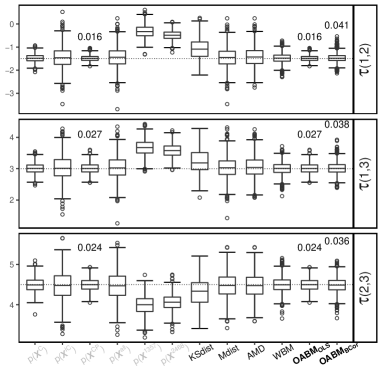
(a) $u=2,v=1$
Outcome linear in covariates

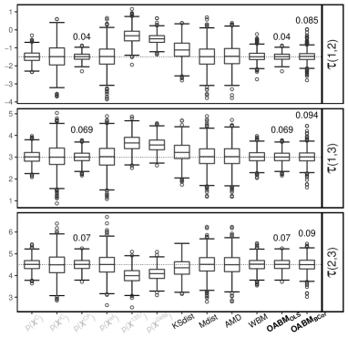
(b) $u=2,v=2$
Outcome linear in covariates

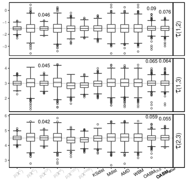
(c) $u=2,v=1$
Outcome nonlinear in covariates

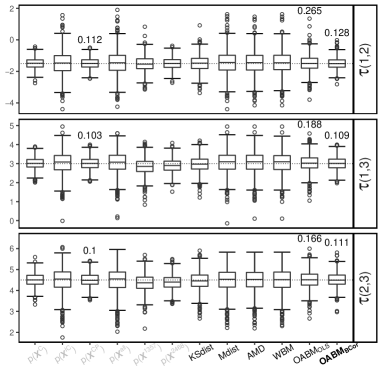
(d) $u=2,v=2$
Outcome nonlinear in covariates

Figure 2: Box plots of 1000 generalized propensity score matching estimates under 2 linear and 2 nonlinear scenarios. The 6 benchmark GPS models are greyed out on the $x$-axis. Numeric MSEs for $\mathtt{p(\bm{X}^{CP})}$, $\mathtt{OABM}_{\mathtt{BCor}}$ and $\mathtt{OABM}_{\mathtt{OLS}}$ are explicitly shown above their corresponding box plots. True pairwise treatment effects are denoted by the horizontal dotted lines.

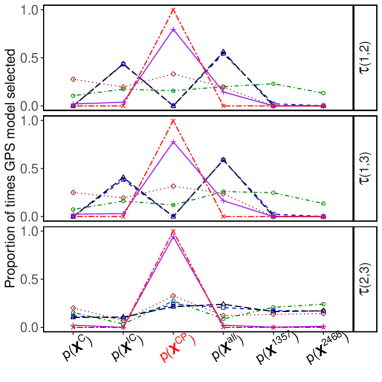
(a) $u=2,v=1$
Outcome linear in covariates

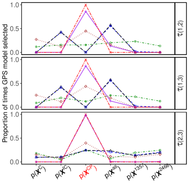
(b) $u=2,v=2$
Outcome linear in covariates

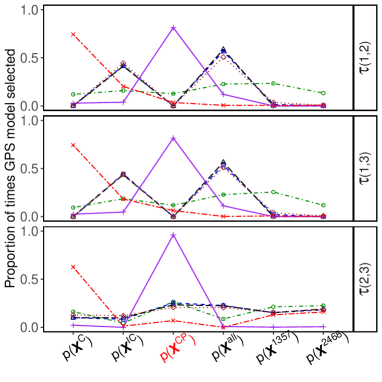
(c) $u=2,v=1$
Outcome nonlinear in covariates

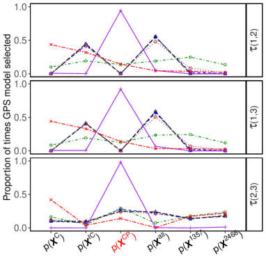
(d) $u=2,v=2$
Outcome nonlinear in covariates

(e)

Figure 3: Proportion of benchmark models selected by the six balance measures over 1000 simulations under 2 linear and 2 nonlinear scenarios. The optimal GPS model is colored red on the $x$-axis.

	$\tau(1,2)$	$\tau(1,3)$	$\tau(2,3)$
$\mathtt{KSdist}$	0.586	0.688	0.725
$\mathtt{Mdist}$	0.908	0.907	0.929
$\mathtt{AMD}$	0.897	0.900	0.911
$\mathtt{WBM}$	0.958	0.963	0.965
$\mathtt{OABM}_{\mathtt{OLS}}$	0.964	0.935	0.950
$\mathtt{OABM}_{\mathtt{BCor}}$	0.954	0.936	0.948

(a) $u=2,v=1$
Outcome linear in covariates

	$\tau(1,2)$	$\tau(1,3)$	$\tau(2,3)$
$\mathtt{KSdist}$	0.744	0.800	0.851
$\mathtt{Mdist}$	0.932	0.898	0.907
$\mathtt{AMD}$	0.918	0.887	0.896
$\mathtt{WBM}$	0.986	0.945	0.950
$\mathtt{OABM}_{\mathtt{OLS}}$	0.987	0.917	0.917
$\mathtt{OABM}_{\mathtt{BCor}}$	0.969	0.916	0.916

(b) $u=2,v=2$
Outcome linear in covariates

	$\tau(1,2)$	$\tau(1,3)$	$\tau(2,3)$
$\mathtt{KSdist}$	0.929	0.939	0.937
$\mathtt{Mdist}$	0.914	0.904	0.898
$\mathtt{AMD}$	0.908	0.905	0.900
$\mathtt{WBM}$	0.900	0.909	0.890
$\mathtt{OABM}_{\mathtt{OLS}}$	0.930	0.937	0.946
$\mathtt{OABM}_{\mathtt{BCor}}$	0.929	0.938	0.934

(c) $u=2,v=1$
Outcome nonlinear in covariates

	$\tau(1,2)$	$\tau(1,3)$	$\tau(2,3)$
$\mathtt{KSdist}$	0.941	0.942	0.932
$\mathtt{Mdist}$	0.905	0.908	0.900
$\mathtt{AMD}$	0.903	0.911	0.903
$\mathtt{WBM}$	0.898	0.920	0.900
$\mathtt{OABM}_{\mathtt{OLS}}$	0.927	0.918	0.935
$\mathtt{OABM}_{\mathtt{BCor}}$	0.941	0.942	0.946

(d) $u=2,v=2$
Outcome nonlinear in covariates

Table 1: Coverage rates of asymptotic 95% confidence intervals under 2 linear and 2 nonlinear scenarios.

Figure 2 summarizes the performance of the GPSM estimator based on the six benchmark models and five measures under the 4 chosen scenarios. Models $\mathtt{p(\bm{X}^{1357})}$ and $\mathtt{p(\bm{X}^{2468})}$ both yield biased estimates in all four scenarios due to failure to include all confounders. While all other benchmark models lead to unbiased estimates, estimates by matching on $\mathtt{p(\bm{X}^{CP})}$ result in the smallest variance. Under the linear outcome design, $\mathtt{OABM}_{\mathtt{OLS}}$ has mean squared error closest to the optimal benchmark model, and outperforms all other measures. $\mathtt{OABM}_{\mathtt{BCor}}$ results in mean squared error smaller than $\mathtt{Mdist}$ and $\mathtt{AMD}$, and performs similar to $\mathtt{WBM}$. Bias occurs when matching on GPS models selected based on $\mathtt{KSdist}$. When the mean potential outcome is nonlinear in the covariates, $\mathtt{OABM}_{\mathtt{OLS}}$ no longer dominates in performance due to the outcome model misspecification. In this case, because of the model-free property of the ball correlation, $\mathtt{OABM}_{\mathtt{BCor}}$ shows a slight advantage over all other measures in terms of MSE. For interval estimation, Table 1 shows that coverage rates for nominal $95\%$ confidence intervals for $\mathtt{OABM}_{\mathtt{BCor}}$ do not deviate much from the specified $95\%$ probability in all four scenarios; Similarly, $\mathtt{OABM}_{\mathtt{OLS}}$ has coverage rates close to the specified $95\%$ when each mean potential outcome is a linear function of the covariates.

In Figure 3 we present the proportion of times each of the six benchmark GPS models are selected by the measures. When outcome is linear in covariates, $\mathtt{OABM}_{\mathtt{OLS}}$ consistently selects $\mathtt{p(\bm{X}^{CP})}$, the GPS model that results in the smallest mean squared error. Following $\mathtt{OABM}_{\mathtt{OLS}}$, $\mathtt{OABM}_{\mathtt{BCor}}$ selects $\mathtt{p(\bm{X}^{CP})}$ with high proportions, while occasionally selecting the benchmark model that includes all covariates. $\mathtt{Mdist}$ and $\mathtt{AMD}$ tend to select GPS models that include the IVs, thereby explaining their large estimation variance. When the potential outcome is nonlinear in the covariates, $\mathtt{OABM}_{\mathtt{OLS}}$ no longer selects $\mathtt{p(\bm{X}^{CP})}$, while $\mathtt{OABM}_{\mathtt{BCor}}$ is still able to identify it thanks to the model-free property of the ball correlation. In this case, in addition to $\mathtt{Mdist}$ and $\mathtt{AMD}$, $\mathtt{WBM}$ also frequently selects GPS models that include the instrumental variables. $\mathtt{KSdist}$’s worst performance in estimation could be explained by its inability to rule out the two biased benchmark models.

6 An Application

We apply the model selection method to the Tutoring dataset from the TriMatch R package (Bryer,, 2017), which contains results from a study examining the effects of tutoring services on course grades. A total of 1172 observations consist of 918 students who did not receive any form of tutoring (Control), 134 students who received the first form of tutoring (Treat1), and 90 students who received the second form of tutoring (Treat2). The course grade the student earn is the outcome variable and takes on one of five numeric values: 4=A, 3=B, 2=C, 1=D, 0=F or W. Information on gender, ethnicity, military service status of the student, non-native English speaker status, education level of the student’s mother, education level of the student’s father, age of the student, employment status, household income, number of transfer credits, and grade point average are collected as baseline covariates. The objective in this analysis is to posit and select the best generalized propensity score models using the outcome-adjusted balance measure. The fitted generalized propensity scores (probabilities of a student receiving each of the three tutoring services) will serve as matching variables for the GPSM estimator to estimate and make inference about the pairwise average treatment effects.

We add all first order interaction and second order terms to the original 11 covariates to form a total of 84 covariates. We apply the group lasso (Yuan and Lin,, 2006) and select 10 covariates that are strong predictors for tutoring service assignment. We also apply the lasso and selected 26 covariates for predicting $Y(\text{Control})$, 11 for predicting $Y(\text{Treat1})$, and 4 for predicting $Y(\text{Treat2})$. For estimation of $\mathbb{E}\left\{Y(\text{Control})\right\}$, we tentatively categorize the relevant covariates into 6 instrumental variables, 4 confounders, and 22 precision variables based on the lasso variable selection results. We follow the same procedure to partition the relevant covariates for estimation of $\mathbb{E}\left\{Y(\text{Treat1})\right\}$ into 10 instrumental variables, 0 confounders, and lastly 11 precision variables, and 10 instrumental variables, 0 confounders, and 4 precision variables for estimating $\mathbb{E}\left\{Y(\text{Treat2})\right\}$.

For each treatment level $w$, we estimate the average potential outcome $\mathbb{E}\left\{Y(w)\right\}$ by positing the following three candidate GPS models:

• Model 1: multinomial logit with all relevant covariates entering linearly

• Model 2: multinomial logit with confounders and precision variables entering linearly

• Model 3: multinomial logit with confounders and top 3 precision variables ranked by lasso coefficients entering linearly

We consider two versions of the outcome-adjusted balance measure to conduct GPS model selection. First, $\mathtt{OABM}_{\mathtt{BCor}}$ uses the ball correlation to construct the penalty weights in the outcome-adjusted balance measure; it represents our lack of confidence in describing the true relationship between the full set of covariates and the course grades conditional on the choice of tutoring service. On the other hand, since the outcome is ordinal, the ordinal probit model ($\mathtt{OABM}_{\mathtt{OP}}$) could serve as a reasonable approximation to the underlying relationship between the covariates and the outcome conditional on the treatment assignment. We evaluate the two balance measures on the three proposed models for each separate average potential outcome estimation, and the model selection results are shown in Table 2. For estimating $\mathbb{E}\left\{Y(\text{Treat1})\right\}$ and $\mathbb{E}\left\{Y(\text{Treat2})\right\}$, two variants of $\mathtt{OABM}_{\rho}$ both select Model 3. For estimating $\mathbb{E}\left\{Y(\text{Control})\right\}$, $\mathtt{OABM}_{\mathtt{BCor}}$ picks the most conservative Model 1, while $\mathtt{OABM}_{\mathtt{OP}}$ selects Model 3. The selected model specifications are subsequently used to fit the data and compute the estimated generalized propensity scores, which serve as matching variables for the GPSM estimator to produce point estimates and 95% confidence intervals for the pairwise ATEs, as shown in Table 3. Since none of the confidence intervals contains zero, there is sufficient statistical evidence that students undergoing the second form of tutoring will have better course grades than if they receive the first form of tutoring or no tutoring at all. Receiving the first form of tutoring also seems to help increase course grades compared to not receiving any form of tutoring at all.

	$\mathbb{E}[Y(Control)]$		$\mathbb{E}[Y(Treat1)]$		$\mathbb{E}[Y(Treat2)]$
Model	$\mathtt{OABM}_{\mathtt{BCor}}$	$\mathtt{OABM}_{\mathtt{OP}}$	$\mathtt{OABM}_{\mathtt{BCor}}$	$\mathtt{OABM}_{\mathtt{OP}}$	$\mathtt{OABM}_{\mathtt{BCor}}$	$\mathtt{OABM}_{\mathtt{OP}}$
1	115.69	5.12	173.38	42.36	108.99	11.07
2	197.76	9.11	71.83	3.46	18.64	43.50
3	222.08	1.58	26.01	2.79	33.65	5.20

Table 2: GPS model selection results; the smallest balance measures based on $\mathtt{OABM}_{\mathtt{BCor}}$ are highlighted in red, and those based on $\mathtt{OABM}_{\mathtt{OP}}$ are highlighted in orange.

Measure	$\widehat{\mathbb{E}}\left\{Y(\text{Treat1})-Y(\text{Control})\right\}$	$\widehat{\mathbb{E}}\left\{Y(\text{Treat2})-Y(\text{Control})\right\}$	$\widehat{\mathbb{E}}\left\{Y(\text{Treat2})-Y(\text{Treat1})\right\}$
$\mathtt{OABM}_{\mathtt{BCor}}$	0.35(0.14, 0.56)	0.66(0.47, 0.85)	0.31(0.08, 0.55)
$\mathtt{OABM}_{\mathtt{OP}}$	0.31(0.10, 0.52)	0.63(0.46, 0.81)	0.33(0.09, 0.56)

Table 3: Pairwise ATE estimates (95% CI)

7 Discussion

In this article, we present a novel balance measure that can select the optimal generalized propensity score model from a set of candidate models for the estimation of each average potential outcome. Given a set of candidate GPS models, the outcome-adjusted balance measure works as follows. First we impute all measured covariates by matching on each candidate GPS model as if they were missing. For each candidate model, the balance measure then evaluates a weighted sum of the absolute mean differences between the imputed covariates and their original sample values. These absolute differences are each scaled by a penalty, which takes into account the covariate’s relationship with the potential outcome to ensure that only the desired covariates are selected into the GPS model. Under certain conditions, we theoretically show that in large samples, the GPS specification that minimizes the proposed balance measure is the optimal GPS model. As a result, the GPSM estimator based on a GPS model selected by the outcome-adjusted balance measure is consistent and efficient for the pairwise ATEs.

Since the proposed balance measure incorporates outcome information to conduct GPS model selection, this is contradictory to Rubin’s principle that modeling of the assignment mechanism should be carried out at the design stage, without accessing any outcomes (Rubin,, 2007). However, for efficiency considerations, leveraging outcome information is necessary. In practice, if pilot studies exist, the outcome information can be borrowed from existing studies.

In addition to limitations shared by all (G)PS based methods such as the existence of unmeasured confounders, we review some possible limitations specific to the outcome-adjusted balance measure. First, as discussed in previous sections, when the outcome model cannot be well characterized, model selection consistency for the outcome-adjusted balance measure based on the ball correlation only holds approximately, depending on how large the collider bias is. Similarly, $\mathtt{OABM_{BCor}}$ is also unable to exclude a noise variable that is a collider of instrumental variables and precision variables, a scenario commonly known as the M-Bias structure. Including this noise variable in the GPS model will introduce bias in estimating the ATE. Despite these theoretical anomalies, it is rarely the case that the magnitude of the collider bias described above will be substantial in practice (Ding and Miratrix,, 2014). Lastly, the success of balance measure relies on the fact that the set of posited GPS models must contain the optimally specified model or at least one close approximation to it. If the set of posited GPS models only consists of severely misspecified models, then the balance measure may not be able to suggest the "best" one among them.

Future research work may involve extending the current balance measure to settings with longitudinal or time-to-event outcomes (Tang et al., 2020b, ), as well as to predictive mean matching (Yang and Kim,, 2020) in missing data, where the predictive mean function requires estimation and model selection.

References

- Abadie and Imbens, (2016) Abadie, A. and Imbens, G. W. (2016). Matching on the estimated propensity score. Econometrica, 84(2):781–807.
- Ali et al., (2014) Ali, M. S., Groenwold, R. H., Pestman, W. R., Belitser, S. V., Roes, K. C., Hoes, A. W., de Boer, A., and Klungel, O. H. (2014). Propensity score balance measures in pharmacoepidemiology: a simulation study. Pharmacoepidemiology and drug safety, 23(8):802–811.
- Austin, (2009) Austin, P. C. (2009). Balance diagnostics for comparing the distribution of baseline covariates between treatment groups in propensity-score matched samples. Statistics in Medicine, 28(25):3083–3107.
- Austin et al., (2007) Austin, P. C., Grootendorst, P., and Anderson, G. M. (2007). A comparison of the ability of different propensity score models to balance measured variables between treated and untreated subjects: A Monte Carlo study. Statistics in Medicine, 26(4):734–753.
- Belitser et al., (2011) Belitser, S. V., Martens, E. P., Pestman, W. R., Groenwold, R. H., Boer, A., and Klungel, O. H. (2011). Measuring balance and model selection in propensity score methods: BALANCE MEASURE FOR PROPENSITY SCORES METHODS. Pharmacoepidemiology and Drug Safety, 20(11):1115–1129.
- Brookhart et al., (2006) Brookhart, M. A., Schneeweiss, S., Rothman, K. J., Glynn, R. J., Avorn, J., and Stürmer, T. (2006). Variable Selection for Propensity Score Models. American Journal of Epidemiology, 163(12):1149–1156.
- Bryer, (2017) Bryer, J. (2017). TriMatch: Propensity Score Matching of Non-Binary Treatments. R package version 0.9.9.
- Caruana et al., (2015) Caruana, E., Chevret, S., Resche-Rigon, M., and Pirracchio, R. (2015). A new weighted balance measure helped to select the variables to be included in a propensity score model. Journal of Clinical Epidemiology, 68(12):1415–1422.e2.
- Ding and Miratrix, (2014) Ding, P. and Miratrix, L. (2014). To adjust or not to adjust? sensitivity analysis of m-bias and butterfly-bias.
- Hahn, (2004) Hahn, J. (2004). Functional Restriction and Efficiency in Causal Inference. The Review of Economics and Statistics, 86(1):73–76.
- Imbens, (2000) Imbens, G. W. (2000). The Role of the Propensity Score in Estimating Dose-Response Functions. Biometrika, 87(3):706–710.
- Ju et al., (2019) Ju, C., Wyss, R., Franklin, J. M., Schneeweiss, S., Häggström, J., and van der Laan, M. J. (2019). Collaborative-controlled lasso for constructing propensity score-based estimators in high-dimensional data. Statistical methods in medical research, 28(4):1044–1063.
- Lunceford and Davidian, (2004) Lunceford, J. K. and Davidian, M. (2004). Stratification and weighting via the propensity score in estimation of causal treatment effects: A comparative study. Statistics in Medicine, 23(19):2937–2960.
- Myers et al., (2011) Myers, J. A., Rassen, J. A., Gagne, J. J., Huybrechts, K. F., Schneeweiss, S., Rothman, K. J., Joffe, M. M., and Glynn, R. J. (2011). Effects of Adjusting for Instrumental Variables on Bias and Precision of Effect Estimates. American Journal of Epidemiology, 174(11):1213–1222.
- Pan et al., (2020) Pan, W., Wang, X., Zhang, H., Zhu, H., and Zhu, J. (2020). Ball Covariance: A Generic Measure of Dependence in Banach Space. Journal of the American Statistical Association, 115(529):307–317.
- Patrick et al., (2011) Patrick, A. R., Schneeweiss, S., Brookhart, M. A., Glynn, R. J., Rothman, K. J., Avorn, J., and Stürmer, T. (2011). The implications of propensity score variable selection strategies in pharmacoepidemiology: An empirical illustration. Pharmacoepidemiology and Drug Safety, 20(6):551–559.
- Pearl, (2000) Pearl, J. (2000). Causality: Models, Reasoning, and Inference. Causality: Models, Reasoning, and Inference. New York, NY, US.
- Pearl, (2011) Pearl, J. (2011). Invited Commentary: Understanding Bias Amplification. American Journal of Epidemiology, 174(11):1223–1227.
- Rosenbaum and Rubin, (1983) Rosenbaum, P. R. and Rubin, D. B. (1983). The Central Role of the Propensity Score in Observational Studies for Causal Effects. Biometrika, 70(1):41–55.
- Rotnitzky and Smucler, (2019) Rotnitzky, A. and Smucler, E. (2019). Efficient adjustment sets for population average treatment effect estimation in non-parametric causal graphical models. arXiv:1912.00306 [cs, math, stat].
- Rubin, (2007) Rubin, D. B. (2007). The design versus the analysis of observational studies for causal effects: parallels with the design of randomized trials. Statistics in medicine, 26(1):20–36.
- Shortreed and Ertefaie, (2017) Shortreed, S. M. and Ertefaie, A. (2017). Outcome-adaptive lasso: Variable selection for causal inference. Biometrics, 73(4):1111–1122.
- Székely et al., (2007) Székely, G. J., Rizzo, M. L., and Bakirov, N. K. (2007). Measuring and testing dependence by correlation of distances. The annals of statistics, 35(6):2769–2794.
- (24) Tang, D., Kong, D., Pan, W., and Wang, L. (2020a). Outcome model free causal inference with ultra-high dimensional covariates. arXiv:2007.14190 [stat].
- (25) Tang, S., Yang, S., Wang, T., Cui, Z., Li, L., and Faries, D. E. (2020b). Causal inference of hazard ratio based on propensity score matching.
- Westreich et al., (2011) Westreich, D., Cole, S. R., Funk, M. J., Brookhart, M. A., and Stürmer, T. (2011). The role of the c-statistic in variable selection for propensity score models. Pharmacoepidemiology and Drug Safety, 20(3):317–320.
- Yang et al., (2016) Yang, S., Imbens, G. W., Cui, Z., Faries, D. E., and Kadziola, Z. (2016). Propensity score matching and subclassification in observational studies with multi-level treatments. Biometrics, 72(4):1055–1065.
- Yang and Kim, (2020) Yang, S. and Kim, J. K. (2020). Asymptotic theory and inference of predictive mean matching imputation using a superpopulation model framework. Scandinavian Journal of Statistics, 47(3):839–861.
- Yuan and Lin, (2006) Yuan, M. and Lin, Y. (2006). Model Selection and Estimation in Regression With Grouped Variables. Journal of the Royal Statistical Society Series B, 68:49–67.