Residence time in presence of moving defects and obstacles

Abstract

We discuss the properties of the residence time in presence of moving defects or obstacles for a particle performing a one dimensional random walk. More precisely, for a particle conditioned to exit through the right endpoint, we measure the typical time needed to cross the entire lattice in presence of defects. We find explicit formulae for the residence time and discuss several models of moving obstacles. The presence of a stochastic updating rule for the motion of the obstacle smoothens the local residence time profiles found in the case of a static obstacle. We finally discuss connections with applicative problems, such as the pedestrian motion in presence of queues and the residence time of water flows in runoff ponds.

Keywords: residence time, random walk, moving obstacles

1 Introduction

The characterization of transport regimes in presence of obstacles and irregular patterns is a classical problem of fluid dynamics [1, 2], which is also relevant to a number of biological [3] and engineering [4, 5] applications. For instance, a careful design of the shape and the location of the obstacles in microfluidic channels was observed to enhance the mixing of fluid flows [6]. Moreover, crowding effects, generated by obstacles of different size and shape, turn out to significantly affect the transport properties by even altering the sign of the fluxes, as recently reported, e.g., in active matter numerical experiments [7, 8].

From the perspective of statistical mechanics, the subject is particularly rich and may be tackled from different routes. One first important question, for instance, concerns the study of anomalous diffusions resulting from the presence of obstacles [9, 10]. The onset of anomalous transport stemming from the motion of intruders in a host matrix of slowly moving particles was studied in [11]. The inclusion of flower shape obstacles in billiards was considered in [12] in order to highlight the fractal structure of the diffusion coefficient as a function of control parameters. Another interesting research line concerns the derivation of the hydrodynamic limit of interacting particle systems in an inhomogeneous environment. In [13] it was shown that a detailed characterization of the inhomogeneities at the microscopic level is necessary to determine the structure of the macroscopic diffusion laws in the hydrodynamic limit. Furthermore, in the framework of Zero Range Processes, the inclusion of local defects proved to be a mechanism able to give rise to condensation phenomena in the hydrodynamic limit [14].

The investigation of inhomogeneous random walks continues to be a core topic in statistical mechanics, see e.g. [15] for a general review of the subject.

In this work we study the residence time in a random walk on a one-dimensional lattice in presence of local inhomogeneities. The walker is conditioned to exit through the right endpoint of the lane. Our approach permits explicit computations that nicely complement the classical literature based on the gambler’s ruin problem. We consider both symmetric and asymmetric random walks, and discuss the residence time in presence of defects, represented by lattice sites on which the hopping probabilities of the walker are perturbed by a bias. In particular, analytical formulae for the residence time are obtained for random walks with static defects as well as in presence of defects following a stochastic updating rule.

By exploiting the theory of absorbing Markov chains, we succeed, to a certain general extent, to express the residence time of the conditioned random walk in terms of quantities evaluated in the non conditioned walk: the mean number of visits on the generic site of the lattice and the right exit probability. Thus, we dwell on the derivation of analytic formulae for these two quantities and use them to write explicit formulae for the residence time in presence of static defects. The prominent effect of the inclusion of a defect obeying a stochastic dynamics is the smoothing of the local residence time profiles. Our analysis, supported by numerical simulations, also shows that the presence of a stochastic defect may induce a decrease of the residence time. Moreover, for certain distributions of the defect, the residence time turns out to be invariant with respect to the sign of the bias acting on the defect.

Our results are also amenable to a variety of applications. We discuss, in particular, the use of our formalism in the modelling of pedestrians forming queues and also outline useful links with hydrogeological problems. In both cases, we show that the results found in those contexts by means of sophisticated models can be recovered to some extent in the framework of our one dimensional random walk model through a suitable choice of the parameters.

In addition, we show in the Appendix how our results on the stationary local residence time profile connect with the stationary fugacity profiles of arbitrary Zero Range Processes subject to specific injection rates at the boundaries.

Our work is organized as follows. In Sec. 2, we introduce the theoretical set-up for the computation of the residence time, based on the fundamental matrix, and define the main quantities of interest. In Sec. 3 we apply our formalism to both symmetric and asymmetric random walks and obtain explicit formulae in presence of static defects. In Sec. 4 we study the residence time problem in presence of moving defects which follow a stochastic updating rule. The discussion of relevant applications and our conclusions are deferred to Sec. 5, while the analogy with Zero Range Processes is outlined in the Appendix A.

2 Model and quantities of interest

The problem discussed above is approached in this paper via a one–dimensional model based on a simple random walk. At each side of the lattice an absorbing site is present. We shall first consider a completely general simple random walk and then we will specialize our discussion to particular models describing the effect of static or moving defects.

We thus consider a one–dimensional simple random walk on $\{0,1,\dots,L\}$, called lane. Each element of the lane will be called site. The sites $0$ and $L$ are absorbing, so that when the particle reaches one of them the walk is stopped. They will be called, respectively, the left and right exit of the lane. The sites $1,\dots,L-1$ are called transient.

Time $t=0,1,2,\dots$ is discrete and at each time the walker jumps from a transient site $i$ to site $j$ with probability $p_{ij}$. We assume $p_{ij}=0$ if $|i-j|=0$ or $|i-j|\geq 2$ and $p_{ij}>0$ otherwise. Moreover, we shall use the notation $p_{ii+1}=p_{i}$ and $p_{ii-1}=q_{i}$, for any $i=1,\dots,L-1$. We will obviously have that $p_{i}+q_{i}=1$. In other words, at each time the walker jumps from the transient site $i$ to its left neighbor $i-1$ with probability $q_{i}$ or to its right neighbor $i+1$ with probability $p_{i}=1-q_{i}$.

We denote by $X(t)$ the position of the walker at time $t$ and by $\mathbb{P}_{i}$ and $\mathbb{E}_{i}$ the probability associated to the process and the related expected value operator for the walk started at $X(0)=i$, with $i=1,\dots,L-1$.

We denote by $Q$ the $(L-1)\times(L-1)$ square matrix in which we collect the transition probabilities between transient sites, namely, $Q_{ij}=p_{ij}$ for $i,j=1,\dots L-1$. The matrix

$$\mathbb{I}-Q=\begin{bmatrix}1&-p_{1}&0&\cdots\\ -q_{2}&1&-p_{2}&0&\cdots\\ 0&-q_{3}&1&-p_{3}&0&\cdots\\ \vdots&&&\ddots\\ &&\cdots&0&-q_{L-2}&1&-p_{L-2}\\ &&&\cdots&0&-q_{L-1}&1\end{bmatrix}$$ (2.1)

is invertible, see, for instance, [16, Theorem 3.2.1], and its inverse $N=(\mathbb{I}-Q)^{-1}$ is called the fundamental matrix.

2.1 Residence time

The residence time is defined by starting the walk at site $1$ and computing the typical time that the particle takes to reach the site $L$ provided the walker reaches $L$ before $0$. More precisely, we denote by $\tau=\inf\{t>0:\,X(t)\in\{0,L\}\}$ the duration of the walk and define the residence time, as

$$\Gamma=\mathbb{E}_{1}(\tau|\textup{RE}),$$ (2.2)

where we conditioned to the event RE meaning that the particle exits the lane through the right exit in $L$.

We shall compute the residence time following ideas differing from the approaches already developed in [17, 18, 19]. In particular, we shall exploit several properties of the fundamental matrix of absorbing Markov chains [16] that will allow us in Section 3 to derive remarkable explicit formulae.

Given a site $i$, the number of visits $n_{i}=|\{t>0:X(t)=i\}|$ to $i$ counts the number of times that the walker visits the site $i$. Its mean value for the walk started at site $j$ can be computed using the fundamental matrix, indeed one has that $\mathbb{E}_{j}[n_{i}]=N_{ji}$, see [16, Theorem 3.2.4]. The mean number of visits of the walker started at $1$ conditioned to the event that it exits the lane in $L$, namely, $\mathbb{E}_{1}[n_{i}|\textup{RE}]$, is called local residence time at $i$. Since, for the walker started at $1$, $\tau=\sum_{i=1}^{L-1}n_{i}$, the residence time can be written as sum of the local residence times, namely,

$$\Gamma=\sum_{i=1}^{L-1}\mathbb{E}_{1}[n_{i}|\textup{RE}].$$ (2.3)

Using the standard theory of absorbing Markov chains it is possible to get rid of the conditioning, as it is can be proven that

$$\mathbb{E}_{1}[n_{i}|\textup{RE}]=\frac{\mathbb{P}_{i}[\textup{RE}]}{\mathbb{P}_{1}[\textup{RE}]}\;\mathbb{E}_{1}[n_{i}].$$ (2.4)

Indeed, we consider the random walk conditioned to exit the lane in $L$, which is a Markov chain with the single absorbing state $L$. The fundamental matrix of such a random walk, see [16, Chapter III, page 65], is given by $D^{-1}ND$, where $D$ is the $(L-1)\times(L-1)$ diagonal matrix whose elements are $\mathbb{P}_{i}[\textup{RE}]$ for $i=1,\dots,L-1$. The inverse $D^{-1}$ is diagonal and its elements are $1/\mathbb{P}_{i}[\textup{RE}]$. Thus, for $i$ fixed

$$(D^{-1}ND)_{1i}=D^{-1}_{1s}N_{sr}D_{ri}=\frac{1}{\mathbb{P}_{1}[\textup{RE}]}N_{1r}D_{ri}=\frac{1}{\mathbb{P}_{1}[\textup{RE}]}N_{1i}\mathbb{P}_{i}[\textup{RE}],$$

which proves (2.4).

Using the equality (2.4) the residence time computation can be reduced to the computation of properties of the non conditioned random walk, indeed

$$\Gamma=\frac{1}{\mathbb{P}_{1}[\textup{RE}]}\sum_{i=1}^{L-1}\mathbb{P}_{i}[\textup{RE}]\mathbb{E}_{1}[n_{i}].$$ (2.5)

2.2 Mean number of visits

Since, as mentioned above, $\mathbb{E}_{1}[n_{i}]=N_{1i}$, in order to compute the mean number of visits of the walker at the generic transient site $i$, we have to compute the first raw of the fundamental matrix, which, we recall, is the inverse of the tridiagonal matrix $\mathbb{I}-Q$ given in (2.1). This can be done in several different ways, here we follow the approach proposed in [20], which will show to be very powerful to deduce the explicit formulae that we shall derive in Section 3. Moreover, this approach will also allow an elegant derivation of the analogy that we shall discuss in the Appendix A.

First we note that from [20, equation (1.2)] the determinant of the matrix $\mathbb{I}-Q$ is equal to the last term $\theta_{L-1}$ of the sequence $\theta_{i}$ defined by the following recursive equations

$$\left\{\begin{array}[]{l}\theta_{i}=\theta_{i-1}-q_{i}p_{i-1}\theta_{i-2}\;\;\;\;i=1,2,\dots,L-1\\ \theta_{-1}=0,\;\theta_{0}=1.\end{array}\right.$$ (2.6)

We borrow from [20] also the definition of the sequence $\phi_{i}$ given through the recursive equations

$$\left\{\begin{array}[]{l}\phi_{i}=\phi_{i+1}-q_{i+1}p_{i}\phi_{i+2}\;\;\;\;i=L-1,L-2,\dots,2,1\\ \phi_{L}=1,\;\phi_{L+1}=0.\end{array}\right.$$ (2.7)

The sequences $\theta_{i}$ and $\phi_{i}$ are not independent, indeed, [20, Lemma 2] states that

$$\theta_{i}\phi_{i+1}-q_{i+1}p_{i}\theta_{i-1}\phi_{i+2}=\theta_{L-1}\;\;\;\;i=L-1,L-2,\dots,2,1.$$ (2.8)

In particular, since from (2.6) $\theta_{1}=1$, comparing (2.8) and (2.7) both for $i=1$, we get

$$\phi_{1}=\theta_{L-1}.$$ (2.9)

Now, by using [20, Lemma 4 and Theorem 2] and exploiting the equality (2.9), we have that

$$N_{1i}=\frac{1}{\phi_{1}}\phi_{i+1}\prod_{k=1}^{i-1}p_{k}\;\;\;\;\;\;i=1,\dots,L-1.$$ (2.10)

Equations (2.10) and (2.7) can be combined to derive a set of recursive equations for $N_{1j}$. Indeed, using (2.7) for $i=1$ and (2.10) for $i=1,2$, we have

$$1=\frac{1}{\phi_{1}}\phi_{2}-\frac{1}{\phi_{1}}q_{2}p_{1}\phi_{3}=N_{11}-q_{2}N_{12}.$$ (2.11)

Using (2.7) for $i=L-1$, and (2.10) for $i=L-1,L-2$, we get

$$\phi_{L-1}=1\Rightarrow\frac{1}{\phi_{1}}\phi_{L-1}\prod_{k=1}^{L-3}p_{k}=\frac{1}{\phi_{1}}\prod_{k=1}^{L-3}p_{k}\Rightarrow N_{1L-2}=\frac{1}{p_{L-2}}N_{1L-1}.$$ (2.12)

Now, we consider (2.7) for $i=L-2,\dots,2$ and multiply it for a suitable coefficient to obtain

$$\frac{1}{\phi_{1}}\phi_{i}\prod_{k=1}^{i-1}p_{k}=\frac{1}{\phi_{1}}\phi_{i+1}\prod_{k=1}^{i-1}p_{k}-q_{i+1}p_{i}\frac{1}{\phi_{1}}\phi_{i+2}\prod_{k=1}^{i-1}p_{k}.$$

Exploiting (2.10) for $i=L-1,L-2,\dots,1$, we get

$$N_{1i-1}p_{i-1}=N_{1i}-q_{i+1}N_{1i+1}.$$ (2.13)

The derivation of equations (2.13) is the key point of our computation: the recursive equations for $\theta_{i}$ and $\phi_{i}$, thanks to the introduction of $N_{1i}$, have been recast in a form which can be easily solved once it is rewritten in the form of a current conservation law. Indeed, by exploiting the fact that $p_{i}+q_{i}=1$, we rewrite the whole set of equations (2.11)–(2.13) as

$$1-q_{1}N_{11}=p_{1}N_{11}-q_{2}N_{12}=\cdots=p_{L-2}N_{1L-2}-q_{L-1}N_{1L-1}=p_{L-1}N_{1L-1}.$$ (2.14)

Thus, the recursive equations (2.13), together with the boundary equations (2.11) and (2.12), allow to find the mean visit number profile $N_{1i}$ for $i=1,\dots,L-1$.

We denote by $c$ the conserved quantity defined by equations (2.14) and solve by induction the first $L-1$ equations

$$1-q_{1}N_{11}=p_{1}N_{11}-q_{2}N_{12}=\cdots=p_{L-2}N_{1L-2}-q_{L-1}N_{1L-1}=c$$

obtaining

$$N_{1i}=\frac{\prod_{k=1}^{i-1}p_{k}}{\prod_{k=1}^{i}q_{k}}-c\sum_{s=0}^{i-1}\frac{\prod_{k=s+1}^{i-1}p_{k}}{\prod_{k=s+1}^{i}q_{k}}\;\;\;\;\;i=1,\dots,L-1.$$ (2.15)

The last equation $p_{L-1}N_{1L-1}=c$ of the set of equations (2.14) can be then used to set the value of the constant $c$, indeed, from

$$p_{L-1}\bigg{[}\frac{\prod_{k=1}^{L-2}p_{k}}{\prod_{k=1}^{L-1}q_{k}}-c\sum_{s=0}^{L-2}\frac{\prod_{k=s+1}^{L-2}p_{k}}{\prod_{k=s+1}^{L-1}q_{k}}\bigg{]}=c,$$

we get

$$c=\frac{\prod_{k=1}^{L-2}p_{k}}{\prod_{k=1}^{L-1}q_{k}}\bigg{[}\frac{1}{p_{L-1}}+\sum_{s=0}^{L-2}\frac{\prod_{k=s+1}^{L-2}p_{k}}{\prod_{k=s+1}^{L-1}q_{k}}\bigg{]}^{-1}.$$ (2.16)

We remark that, summing $N_{1i}$ for $i=1,\dots,L-1$, one can use (2.15) to compute the total length of the walk that, in the gambler’s ruin language, is the duration of the game. It is a straightforward exercise to show that for the symmetric walk, namely, $p_{i}=q_{i}=1/2$ for $i=1,\dots,L-1$, one finds $c=1/L$ and $N_{1i}=2-2i/L$, so that the duration of the walk is $2\sum_{i=1}^{L-1}(1-i/L)=L-1$, see [21, equation (3.5) in Chapter XIV]. The computation is more involved in the homogeneous driven case, i.e., $p_{i}=p$ and $q_{i}=q$ for $i=1,\dots,L-1$ with $p\neq q$. In such a case one finds $c=(p^{L-2}/q^{L-1})[1/p+(p^{L-2}/q^{L-1})((q/p)^{L-1}-1)/(q/p-1)]^{-1}$ and $N_{1i}=(p^{i-1}/q^{i})[1-c((q/p)^{i}-1)/(q/p-1)]$, and summing from $1$ to $L-1$ we find the length of the walk $1/(q-p)-(L/(q-p))(1-q/p)/(1-(q/p)^{L})$, see [21, equation (3.4) in Chapter XIV].

2.3 Right exit probability

The probability of absorption by one particular absorbing state is a classical topic both in the gambler’s ruin problem [21, 17] and in the absorbing Markov chains literature. Adopting the gambler’s ruin point of view, we let $t_{i}=1-\mathbb{P}_{i}[\textup{RE}]$ be the probability that the walker started at $i$ exits the lane at $0$, namely, the probability that the gambler with initial fortune $i$ is eventually ruined, and we note that

$$\left\{\begin{array}[]{l}t_{i}=q_{i}t_{i-1}+p_{i}t_{i+1}\;\;\;\;i=2,\dots,L-2\\ t_{1}=q_{1}+p_{1}t_{2}\\ t_{L-1}=q_{L-1}t_{L-2}.\\ \end{array}\right.$$ (2.17)

We just mention that the same set of equations can be found taking the absorbing Markov chain point of view, indeed we let $R$ be the $(L-1)\times 1$ column vector collecting the probability to jump from any transient site to $L$, i.e., $R_{i1}=0$ if $i=1,\dots,L-2$ and $R_{L-11}=p_{L-1}$. Moreover, we consider the $(L-1)\times 1$ column vector $B$ such that $B_{i1}=\mathbb{P}_{i}[\textup{RE}]$ is the probability that the walker started at site $i$ ends its walk in $L$. From [16, Theorem 3.3.7] we have that $B=NR$, so that

$$B_{i1}=N_{ij}R_{j1}=N_{iL-1}p_{L-1}.$$ (2.18)

Thus, the computation of the right exit probability is reduced to that of the last column of the fundamental matrix. A computation similar to the one performed in Section 2.2 yields the recursive equations for $B_{i1}$ analogous to (2.17).

Now, we come back to the study of the recursive equations (2.17), which can be rewritten in the more compact form

$$\left\{\begin{array}[]{l}t_{i}=q_{i}t_{i-1}+p_{i}t_{i+1}\;\;\;\;i=1,\dots,L-1\\ t_{0}=1,\;\;t_{L}=0.\\ \end{array}\right.$$ (2.19)

To solve (2.19) we first note that the sequences $s_{i}=1$ and $r_{i}=\sum_{k=1}^{i}\prod_{r=k}^{L-1}p_{r}/q_{r}$ are solutions of the recursive equations, but do not satisfy the boundary conditions (recall the footnote 1). The statement is trivial for $s_{i}$, while it requires some effort for $r_{i}$:

$$q_{i}r_{i-1}+p_{i}r_{i+1}=q_{i}\sum_{k=1}^{i-1}\prod_{r=k}^{L-1}\frac{p_{r}}{q_{r}}+p_{i}\sum_{k=1}^{i+1}\prod_{r=k}^{L-1}\frac{p_{r}}{q_{r}}=q_{i}\sum_{k=1}^{i-1}\prod_{r=k}^{L-1}\frac{p_{r}}{q_{r}}+p_{i}\sum_{k=1}^{i}\prod_{r=k}^{L-1}\frac{p_{r}}{q_{r}}+p_{i}\prod_{r=i+1}^{L-1}\frac{p_{r}}{q_{r}}$$

and thus

$$q_{i}r_{i-1}+p_{i}r_{i+1}=q_{i}\sum_{k=1}^{i-1}\prod_{r=k}^{L-1}\frac{p_{r}}{q_{r}}+p_{i}\sum_{k=1}^{i}\prod_{r=k}^{L-1}\frac{p_{r}}{q_{r}}+q_{i}\prod_{r=i}^{L-1}\frac{p_{k}}{q_{k}}=q_{i}\sum_{k=1}^{i}\prod_{r=k}^{L-1}\frac{p_{r}}{q_{r}}+p_{i}\sum_{k=1}^{i}\prod_{r=k}^{L-1}\frac{p_{r}}{q_{r}},$$

which is equal to $r_{i}$ as $q_{i}+p_{i}=1$. Thus, exploiting the recursive linearity of the equation (2.19), we can look for a solution satisfying the boundary condition in the form $t_{i}=as_{i}+br_{i}$, where $a,b$ are real constants. It is not difficult to verify that $a=1$ and $b=-[1+\sum_{k=1}^{L-1}\prod_{r=k}^{L-1}p_{r}/q_{r}]^{-1}$ do the job, so that the sought for solution of the system (2.19) is

$$t_{i}=1-\frac{1}{1+\sum_{k=1}^{L-1}\prod_{r=k}^{L-1}\frac{p_{r}}{q_{r}}}\sum_{k=1}^{i}\prod_{r=k}^{L-1}\frac{p_{r}}{q_{r}}.$$ (2.20)

It is a straightforward exercise to check that in the homogeneous case, in which the jumping probabilities are the same at each site, the classical results of the gambler’s ruin problem (see, e.g., [21, equations (2.4) and (2.5) in Chapter XIV] or [17, Section 3.1]) are recovered.

Finally, recalling that $t_{i}$ is the probability that the walker started at $i$ exits the lane at $0$, we have that the right exit probability is given by

$$\mathbb{P}_{i}[\textup{RE}]=\frac{1}{1+\sum_{k=1}^{L-1}\prod_{r=k}^{L-1}\frac{p_{r}}{q_{r}}}\sum_{k=1}^{i}\prod_{r=k}^{L-1}\frac{p_{r}}{q_{r}}.$$ (2.21)

3 Explicit expression of the residence time in presence of a static defect

In this section we suppose that all the sites $1,\dots,L-1$ share the same behavior, i.e., they are regular, save for one site called defect [17, 18]. The defect site is the site $2\leq d\leq L-2$. More precisely, we assume that $p_{i}=p$ and $q_{i}=q=1-p$ for all $i=1,\dots,L-1$ such that $i\neq d$ and $p_{d}=\bar{p}$ and $q_{d}=\bar{q}=1-\bar{p}$. We shall also write $\bar{p}=p+\epsilon$ and $\bar{q}=q-\epsilon$, with $\epsilon\in(-p,q)$ called bias. We will call symmetric the case in which $p=q$ and driven that in which $p\neq q$. In the driven case $p-q$ is called drift.

Note that, if $\epsilon=0$ the defect is not present and the classical gambler ruin problem is recovered. The case $\epsilon=-p$ cannot be considered, because it would mean that the walker is reflected to the left with probability one by the defect and, hence, it would never reach the right–end exit in $L$. The case $\epsilon=p$ is meaningful, but rather extreme, indeed, in such a case, the defect pushes the walker to the right with probability one and this means that, once the walker started at $1$ has overcome the defect, it will never come back to the part of the lane on the left of the defect. In any case this case is not covered by our study.

3.1 The symmetric case

We start by computing $c$ given in (2.16). In the first factor all the terms cancel but the one associated with the defect and the last term $q_{L-1}$ at the denominator. The sum in the second factor behaves similarly if $s$ ranges from $0$ to $d-1$. On the other hand, for the remaining $L-2-(d-1)$ terms corresponding to $s$ ranging from $d$ to $L-2$, the ratio results equal to $1/q_{L-1}$. Thus, we have

$$c=\frac{2(1/2+\epsilon)}{(1/2-\epsilon)}\bigg{[}2+\frac{2(1/2+\epsilon)}{(1/2-\epsilon)}d+2(L-2-d+1)\bigg{]}^{-1},$$

which yields

$$c=\frac{1+2\epsilon}{L(1-2\epsilon)+4\epsilon d}.$$ (3.22)

To compute the mean number of visits profile (2.15) we use similar arguments, but we have to distinguish three cases. We get

$$N_{1i}=\left\{\begin{array}[]{ll}2-2ci&\;\;\;\;\;i=1,\dots,d-1\\ {\displaystyle\frac{2}{1-2\epsilon}(1-cd)\vphantom{\bigg{\{}_{\big{\}}}}}&\;\;\;\;\;i=d\\ {\displaystyle\frac{2(1+2\epsilon)}{1-2\epsilon}-c\frac{8\epsilon d}{1-2\epsilon}-2ci\vphantom{\bigg{\{}_{\big{\}}}}}&\;\;\;\;\;i=d+1,\dots,L-1.\\ \end{array}\right.$$ (3.23)

The following step is the computation of the right exit probability. From (2.21), distinguishing two different cases, we have

$$\mathbb{P}_{i}[\textup{RE}]=\left\{\begin{array}[]{ll}{\displaystyle\frac{(1+2\epsilon)i}{L(1-2\epsilon)+4\epsilon d}\vphantom{\bigg{\{}_{\big{\}}}}}&\;\;\;i\leq d\\ {\displaystyle\frac{(1-2\epsilon)i}{L(1-2\epsilon)+4\epsilon d}+\frac{4\epsilon d}{L(1-2\epsilon)+4\epsilon d}}&\;\;\;i>d.\\ \end{array}\right.$$ (3.24)

In view of computing the residence time, we now use (2.4) to give an explicit expression of the local residence time profile:

$$\mathbb{E}_{i}[n_{i}|\textup{RE}]=\left\{\begin{array}[]{ll}2i-2ci^{2}&\;\;\;\;\;i=1,\dots,d-1\\ {\displaystyle\frac{2d}{1-2\epsilon}(1-cd)\vphantom{\bigg{\{}_{\big{\}}}}}&\;\;\;\;\;i=d\\ {\displaystyle\frac{(1-2\epsilon)i+4\epsilon d}{1+2\epsilon}\bigg{[}\frac{2(1+2\epsilon)}{1-2\epsilon}-c\frac{8\epsilon d}{1-2\epsilon}-2ci\bigg{]}\vphantom{\bigg{\{}_{\big{\}}}}}&\;\;\;\;\;i=d+1,\dots,L-1.\\ \end{array}\right.$$ (3.25)

Finally, (2.3) is used to compute the residence time

$$\begin{array}[]{rcl}\Gamma&\!\!=&\!\!{\displaystyle(1-c)(d-1)d+\frac{2d(1-cd)}{1-2\varepsilon}}\\ &&\!\!{\displaystyle-\frac{L-d-1}{3(1-4\epsilon^{2})}(-3d+cd+2cd^{2}-3L-cL+2cdL+2cL^{2}-24d\epsilon-4cd\epsilon}\\ &&\!\!{\displaystyle\phantom{-\frac{L-d-1}{3(1-4\epsilon^{2})}(}+16cd^{2}\epsilon+4cL\epsilon+16cdL\epsilon-8cL^{2}\epsilon-36d\epsilon^{2}+4cd\epsilon^{2}+56cd^{2}\epsilon^{2}}\\ &&\!\!{\displaystyle\phantom{-\frac{L-d-1}{3(1-4\epsilon^{2})}(}+12L\epsilon^{2}-4cL\epsilon^{2}-40cdL\epsilon^{2}+8cL^{2}\epsilon^{2})}\\ &\!\!=&\!\!{\displaystyle\frac{L^{3}(1-2\epsilon)+12d\epsilon L^{2}-L(1+24d^{2}\epsilon-2\epsilon)+16d^{3}\epsilon-4d\epsilon}{3[L(1-2\epsilon)+4\epsilon d]}.}\end{array}$$ (3.26)

The leading term for $L$ large, uniformly in the choice of the other parameters $d$ and $\epsilon$, is $L^{2}/3$. Thus, the presence of the defect does not affect for large $L$ the diffusive character of the walk.

Finally, it is worth noting that equation (3.26), in the case $\epsilon=0$, reduces to the residence time for the symmetric model in absence of defect, namely, for the gambler’s ruin problem. Indeed we get $\Gamma=(L^{2}-1)/3$ as also shown in [18, Section IV.A].

Note that the model presented and analyzed so far is analogous to the one studied by Ciallella et al. in [17]. Fig. 3.1 shows the dependence of the residence time $\Gamma$ on the defect site position $d$ in a symmetric random walk, computed through the use of formula (3.26).

Figure 3.1: Residence time as a function of $d$ for a symmetric random walk (i.e., $p=q=0.5$) for $L=101$. In particular, plain circles, triangles and diamonds refer to the defect intensities $\epsilon=-0.4,\>-0.3,\>-0.2$ respectively, while same symbols but empty refer to $\epsilon=0.4,\>0.3,\>0.2$. The solid line corresponds to the residence time of the system without any defect, namely $\Gamma=3467.7$ time steps.

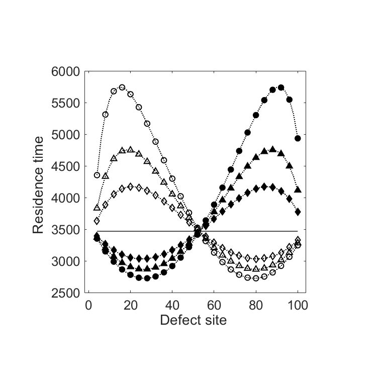
In particular, Fig. 3.1 shows that the behavior of the residence time as a function of the defect site $d$ is analogous to that already observed in [17]. In fact, the residence time is maximized or minimized by the position of the defect, depending on the sign of $\epsilon$, and it is not affected by the defect intensity when $d$ coincides with the central site of the lattice.

3.2 The driven case

We start by computing $c$ given in (2.16). In the first factor all the terms contribute with the ratio $p/q$ but the one associated with the defect, which is $\bar{p}/\bar{q}$, and the last term $q_{L-1}$ at the denominator. The sum in the second factor behaves similarly if $s$ ranges from $0$ to $d-1$. On the other hand, for the remaining $L-2-(d-1)$ terms corresponding to $s$ ranging from $d$ to $L-2$, the ratio results equal to $(p/q)^{L-2-s}(1/q)$.

In order to make the following formulae more compact and legible, we will use the shorthand notation

$$A=\frac{q}{p}\;\;\;\textup{ and }\;\;\;\bar{A}=\frac{\bar{q}}{\bar{p}}.$$

With this convention, we have

$$c=A^{3-L}\frac{1}{\bar{A}}\frac{1}{q}\bigg{[}\frac{1}{p}+\sum_{s=0}^{d-1}A^{s+3-L}\frac{1}{\bar{A}}\frac{1}{q}+\sum_{s=d}^{L-2}A^{s+2-L}\frac{1}{q}\bigg{]}^{-1},$$

which, after some algebra, yields

$$c=A^{3-L}\frac{1}{\bar{A}}\frac{1}{q}\bigg{[}\frac{1}{p}+A^{3-L}\frac{1}{\bar{A}}\frac{1}{q}\frac{A^{d}-1}{A-1}+A^{2-L}\frac{1}{q}\frac{A^{L-1}-A^{d}}{A-1}\bigg{]}^{-1}.$$ (3.27)

To compute the mean number of visits profile (2.15) we use similar arguments, but we have to distinguish three cases. We get

$$N_{1i}=\left\{\begin{array}[]{ll}{\displaystyle A^{1-i}\frac{1}{q}\Big{[}1-c\frac{A^{i}-1}{A-1}\Big{]}\vphantom{\bigg{\{}_{\big{\}}}}}&\;\;\;\;\;i=1,\dots,d-1\\ {\displaystyle A^{1-d}\frac{1}{\bar{q}}\Big{[}1-c\frac{A^{d}-1}{A-1}\Big{]}\vphantom{\bigg{\{}_{\big{\}}}}}&\;\;\;\;\;i=d\\ {\displaystyle A^{2-i}\frac{1}{\bar{A}}\frac{1}{q}-c\Big{[}A^{2-i}\frac{1}{\bar{A}}\frac{1}{q}\frac{A^{d}-1}{A-1}+A^{1-i}\frac{1}{q}\frac{A^{i}-A^{d}}{A-1}\Big{]}\vphantom{\bigg{\{}_{\big{\}}}}}&\;\;\;\;\;i=d+1,\dots,L-1.\\ \end{array}\right.$$ (3.28)

Note that, due to the presence of the term $1/\bar{q}$ in the front factor, the second case is not simply a particularization of the first one.

The following step is the computation of the right exit probability. Although not strictly necessary to derive the expression of the residence time, we first compute the front factor appearing in (2.21):

$$Z=1+\sum_{k=1}^{L-1}\prod_{r=k}^{L-1}\frac{p_{r}}{q_{r}}=1+\frac{1}{\bar{A}A^{L}}\frac{A^{d+1}-A}{A-1}+\frac{1}{A^{L}}\frac{A^{L}-A^{d+1}}{A-1}.$$ (3.29)

Distinguishing two different cases, from (2.21) we have

$$\mathbb{P}_{i}[\textup{RE}]=\left\{\begin{array}[]{ll}{\displaystyle\frac{1}{Z}A^{2-L}\frac{1}{\bar{A}}\frac{A^{i}-1}{A-1}\vphantom{\bigg{\{}_{\big{\}}}}}&\;\;\;i\leq d\\ {\displaystyle\frac{1}{Z}A^{2-L}\Big{[}\frac{1}{\bar{A}}\frac{A^{d}-1}{A-1}+\frac{1}{A^{2}}\frac{A^{i+1}-A^{d+1}}{A-1}\Big{]}}&\;\;\;i>d.\\ \end{array}\right.$$ (3.30)

Using (2.4), (3.28), and (3.30) it is possible to give an explicit formula for the local residence time profile $\mathbb{E}_{i}[n_{i}|\textup{RE}]$ for $i=1,\dots,L-1$. Finally, using (2.3) we compute the residence time that we report here without adopting the shorthand notations $A$ and $\bar{A}$. We have

$$\begin{array}[]{rcl}\Gamma&\!\!=&\!\!{\displaystyle\Big{[}(p-q)^{2}\Big{(}-pq+pq\Big{(}\frac{q}{p}\Big{)}^{L}-q\epsilon-p\Big{(}\frac{q}{p}\Big{)}^{L}\epsilon+\Big{(}\frac{q}{p}\Big{)}^{d}\epsilon\Big{)}\Big{]}^{-1}\Big{(}\frac{q}{p}\Big{)}^{-d}\phantom{\bigg{\{}_{\big{\}}}}}\\ &&\!\!{\displaystyle\times\Big{[}-2pq\Big{(}\frac{q}{p}\Big{)}^{L}\epsilon-\Big{(}\frac{q}{p}\Big{)}^{2d}\Big{(}(1+2d-L)p^{2}+4pq+(1-2d+L)q^{2}\Big{)}\epsilon\phantom{\bigg{\{}_{\big{\}}}}}\\ &&\!\!{\displaystyle\phantom{\times\Big{[}}+\Big{(}\frac{q}{p}\Big{)}^{d}\Big{(}pq(p-Lp+q+Lq)+q(3p-Lp+q+Lq)\epsilon}\\ &&\!\!{\displaystyle\phantom{\times\Big{[}+\Big{(}\frac{q}{p}\Big{)}^{d}\Big{(}}-p\Big{(}\frac{q}{p}\Big{)}^{L}\big{(}(1+L)p(q-\epsilon)+q(q-Lq+(L-3)\epsilon)\big{)}\Big{)}\Big{]}.}\\ &&\!\!{\displaystyle}\\ \end{array}$$ (3.31)

The leading order in $L$, uniformly in the choice of the other parameters $d$ and $\epsilon$, is $L/|p-q|$. Thus, the presence of the defect does not affect the ballistic character of the drifted conditioned walk. It is interesting to remark that this behavior, due to the right conditioning, is conserved also for $q>p$, where in a not conditioned walk we would expect an exponential behavior with $L$ of the mean first hitting time to $L$.

Fig. 3.2 shows the behavior of the residence time $\Gamma$ in a driven random walk as a function of the defect site $d$. In particular, two cases have been distinguished, both with positive drift ($p-q>0$): the first with $\epsilon<0$ and the second with $\epsilon>0$.

Figure 3.2: Residence time as a function of $d$ and of the drift $p-q$, with $p>q$, for a uniformly driven random walk and for $L=101$. The left and right panels refer to the system with $\epsilon=-0.3$ and $\epsilon=0.3$ respectively. In both panels, circles, triangles, diamonds and square refer to $p=0.51,\>0.52,\>0.53,\>0.54$ respectively. Dashed lines refers to the reference residence time for the symmetric random walk (i.e., $p=0.5$), while horizontal solid lines correspond to the residence times of the driven random walks with same values of $p$, but without defects. From the top plot to the bottom one, the no-defect residence times are $\Gamma=2775,\>1926,\>1422,\>1119$ time steps for $p=0.51,\>0.52,\>0.53,\>0.54$ respectively.

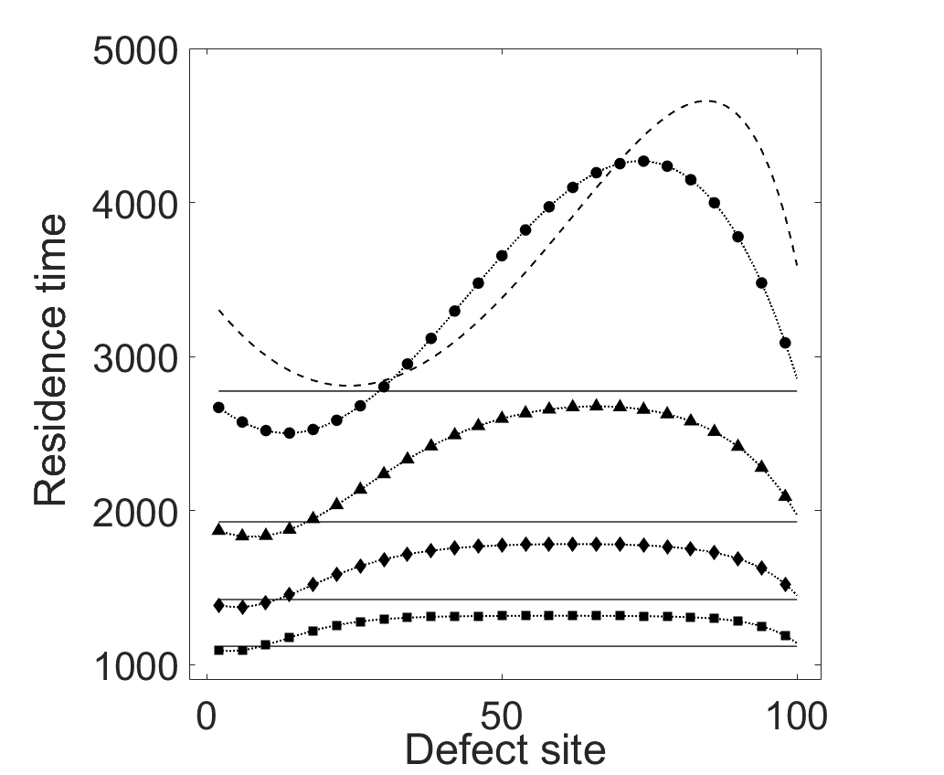
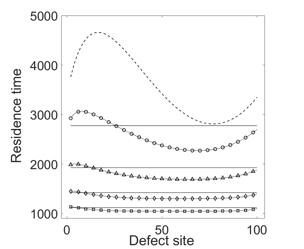
Fig. 3.2 shows how the system with driven random walk and positive drift (i.e., where $p>q$) behaves differently depending on the sign of $\epsilon$, especially for small values of the drift. In particular, in the system characterized by $p>q$ and $\epsilon<0$ it can be noted that for small values of the drift there are intervals of the defect position where the residence time is larger than in the symmetric walk case, despite the drive towards the right exit of the lattice (see Fig.3.2, left panel). In both cases ($\epsilon>0$ and $\epsilon<0$), an increasing value of the drift yields a weaker dependence of the residence time on the position of the defect. In all the cases reported in Fig. 3.2, the residence times have been computed using formula (3.31).

4 Models with one stochastic defect

In the present work, we are interested in studying the effect of different dynamics of the defect on the mean number of visits and on the local and total residence times. Thus the model with static and fixed defect is modified yielding four different versions. The first two are obtained by assuming that the defect is fixed in space, but it is active ($\epsilon\neq 0$) or not ($\epsilon=0$) according to a certain stochastic rule (Models A and B). In the other two, the position of the defect is chosen according to a certain probability distribution over the lattice sites (Models C and D). All the models will be described more in detail and the analytical results obtained in the previous sections are used to derive the mean number of visits and the local and total residence times. These models will be recast as a random walk without defects or with a single static defect through a suitable choice of parameters.

Model A: the defect placed at site $d$ is kept fixed during the random walk, but it is active with probability $\psi$ at each time step. It is immediate to prove that this model generates a behavior which is equivalent to the model with a single static defect at site $d$, where the defect site is characterized by modified jump probabilities, namely $\bar{p}=p+\psi\epsilon$ and $\bar{q}=q-\psi\epsilon$.

Model B: the defect placed at site $d$ is kept fixed during the random walk, but it is active for a random number of time steps (defect is attached to the lattice), sampled from a Poisson distribution of parameter $\lambda_{A}$ and non-active for a random number of time steps (defect is detached from the lattice), sampled from a Poisson distribution of parameter $\lambda_{D}$ [22]. This model generates an average behavior which is equivalent to that of the fixed and static defect model, where the defect site is characterized by jump probabilities $\bar{p}=p+\frac{\lambda_{A}}{\lambda_{A}+\lambda_{D}}\epsilon$ and $\bar{q}=q-\frac{\lambda_{A}}{\lambda_{A}+\lambda_{D}}\epsilon$.

Model C: the defect position is sampled uniformly over the lattice sites at each time step. This model generates a behavior which is equivalent to that of a driven random walk with jump probabilities $\bar{p}=p+\frac{\epsilon}{L}$ and $\bar{q}=q-\frac{\epsilon}{L}$, evolving through a lattice with no defects.

Model D: the defect position is sampled at random from a discrete triangular distribution over the lattice sites at each time step. The triangular distribution is characterized by its mode $d$ and its support $[d-a,d+a]$, with $d-a\geq 2$ and $d+a\leq L-2$. This model generates a behavior which is equivalent to that of a non-homogeneous random walk with jump probabilities $\bar{p}(i)=p+\beta_{i}\epsilon$ and $\bar{q}(i)=q-\beta_{i}\epsilon$, where $\beta_{i}$ is the probability to find the defect at site $i$.

For Models A and B we shall use results provided in Section 3.1 if the walk is symmetric and those of Section 3.2 if the walk is driven. For Model C we use results of Section 3.2 particularized to the case of no defect. Finally, for Model D we will use the general results of Section 2.

Figure 4.3: Mean number of visits and local residence time for Models A and B for $d=51$. Solid lines refer to the random walk model without defects, dash-dotted lines refer to the model with fixed and static defect, empty triangles refer to Model A with $\psi=0.75$, and empty diamonds refer to Model B with $\lambda_{A}=\lambda_{D}=100$. In all cases $\epsilon=0.4$ and $L=101$.

Figure 4.4: Mean number of visits and local residence time for Models A and B. From the top to the bottom $d=26$ and $d=76$. Solid lines refer to the random walk model without defects, dash-dotted lines refer to the model with fixed defect, empty triangles refer to Model A with $\psi=0.75$, and empty diamonds refer to Model B with $\lambda_{A}=\lambda_{D}=100$. In all cases $\epsilon=0.4$ and $L=101$.

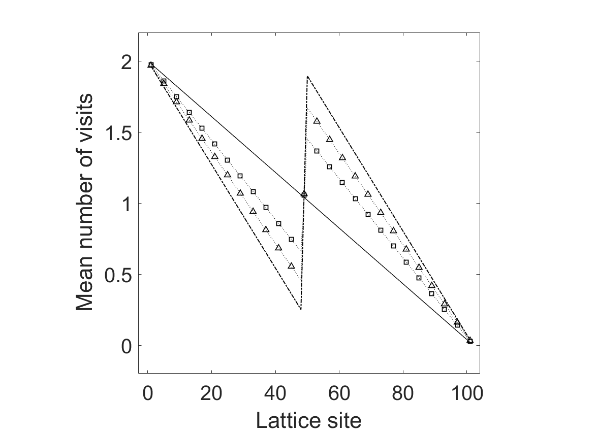
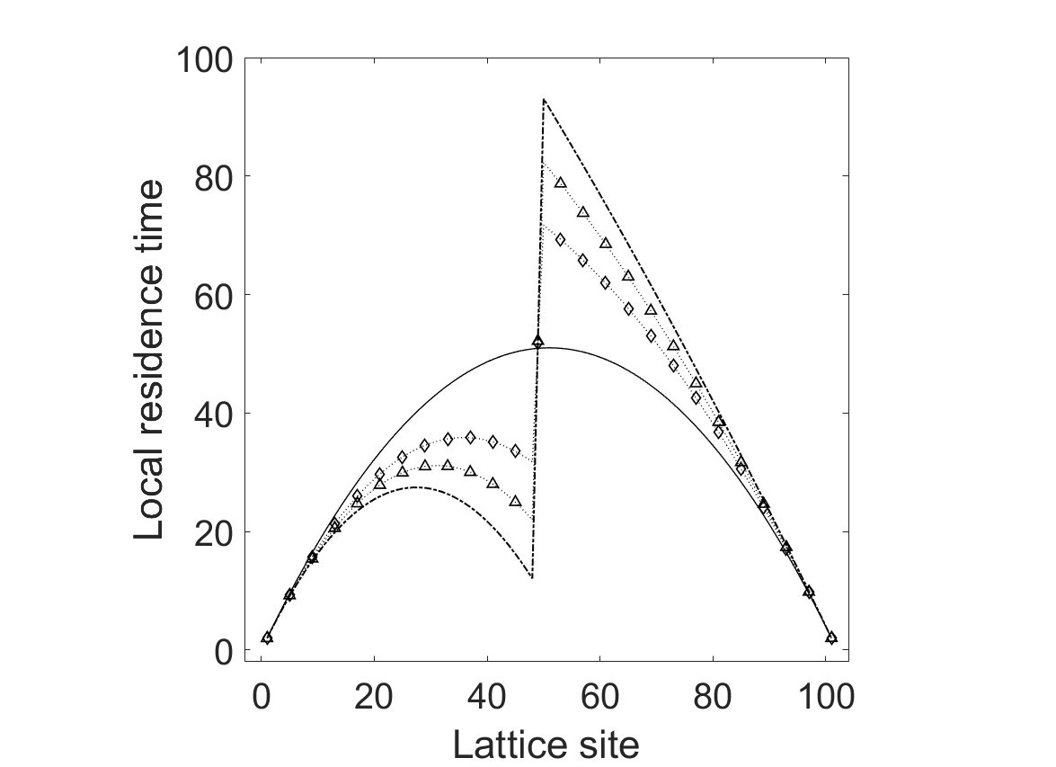
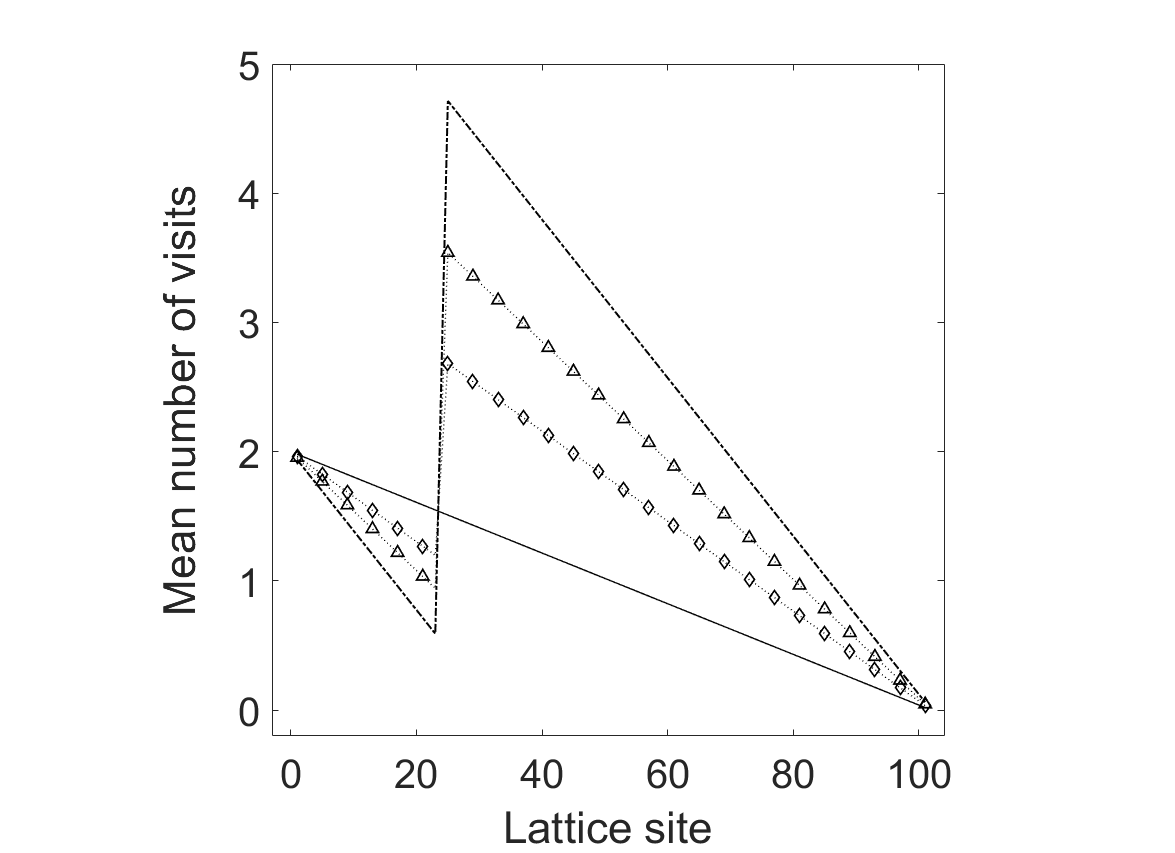
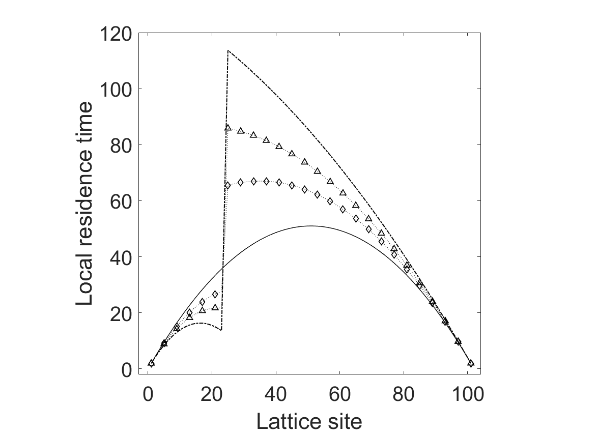
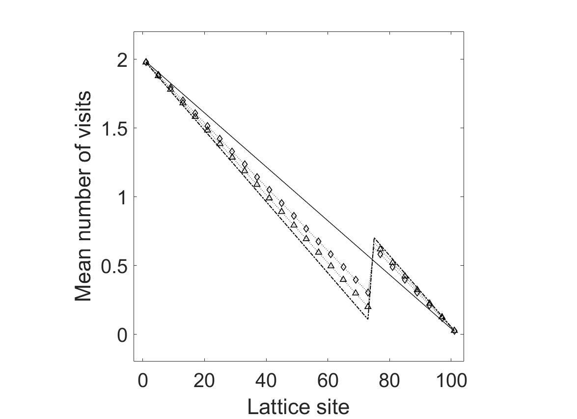
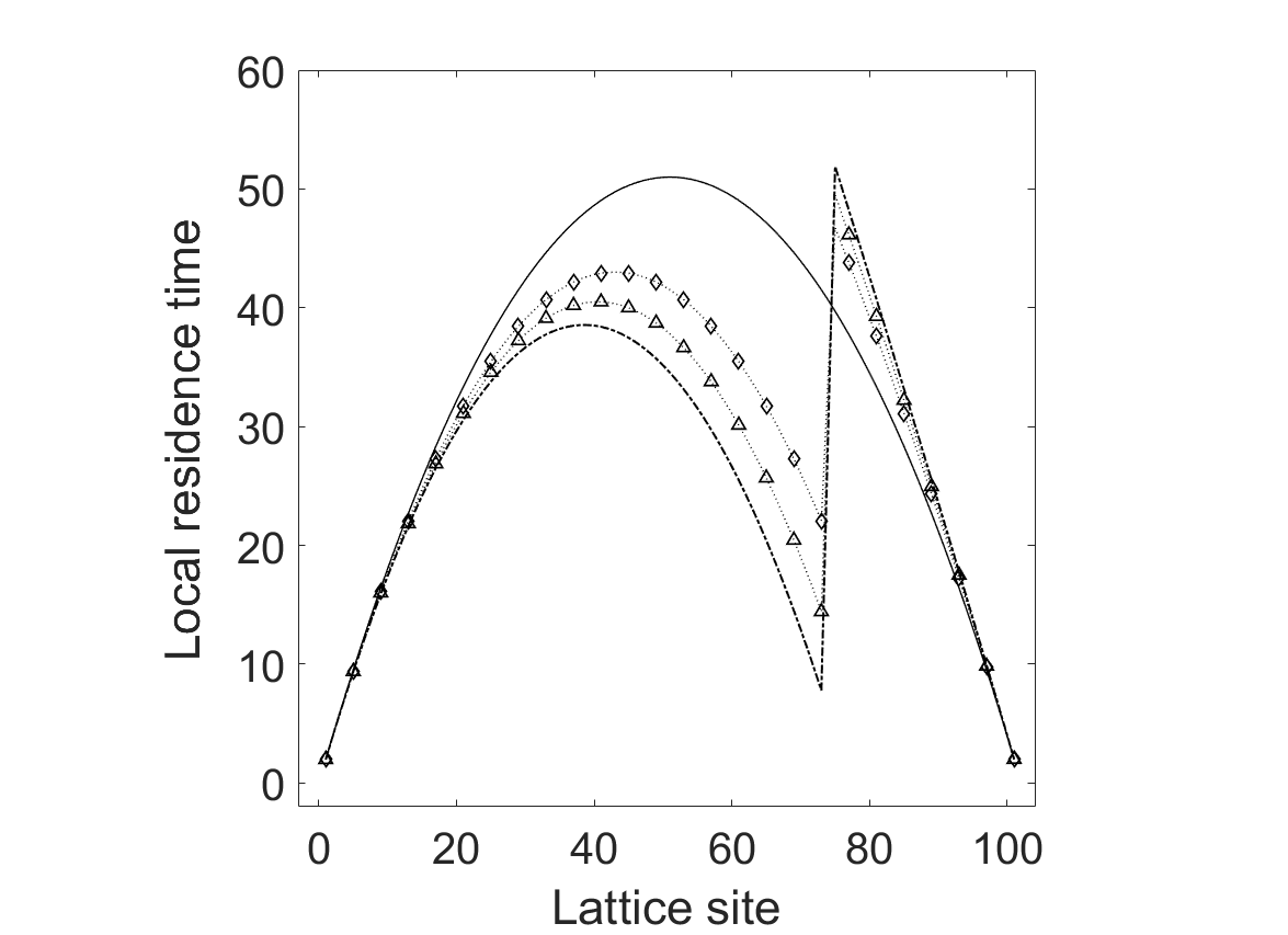
Fig. 4.3 and 4.4 show a comparison in terms of mean number of visits and local residence times between the model with fixed and static defect and Models A and B. Details on the parameters are reported in the figures captions. Notice that the mean number of visits and local residence times have been computed using formulae (3.23) and (3.25) respectively. The lattice has a odd length to account for the possibility of properly defining a central site. It can be observed that adding a stochastic dynamics to the defect results in a reduction of the amplitude of the jump discontinuity in the mean number of visits and in the local residence times profiles. Another remarkable effect of the defect is that on the local residence times (see Fig. 4.3, right panels). In fact, the values of the local residence times and the amplitude of the jump discontinuity are remarkably higher when $d=26$ than when $d=76$. Recalling equation 2.3, it can be seen that this behavior is in agreement to that of $\Gamma$ as a function of $d$ in Fig. 3.1 when $\epsilon>0$, where the asymmetric effect of the defect position on the total residence time is stronger on the left half of the lattice than it is on the right half. In general, residence times for Model A and B behave exactly as those in the fixed and static defect model, except for a proper scaling of $\Gamma$ due to the reduced effectiveness of the defect site (whose intensity is diminished by a factor of $\psi$ or $\frac{\lambda_{A}}{\lambda_{A}+\lambda_{D}}$ for Model A and B respectively).

Figure 4.5: Mean number of visits and local residence times for Model D for different values of $a$ and same metrics for Model C. Dash-dotted lines and asterisks refer to the model with fixed and static defect and to Model C respectively. Triangles, diamonds and squares refer to Model D with $a=5,\>25,\>49$ respectively. All the models are characterized by $\epsilon=0.4$, $d=51$ and $L=101$. Solid lines refer to the no-defect model.

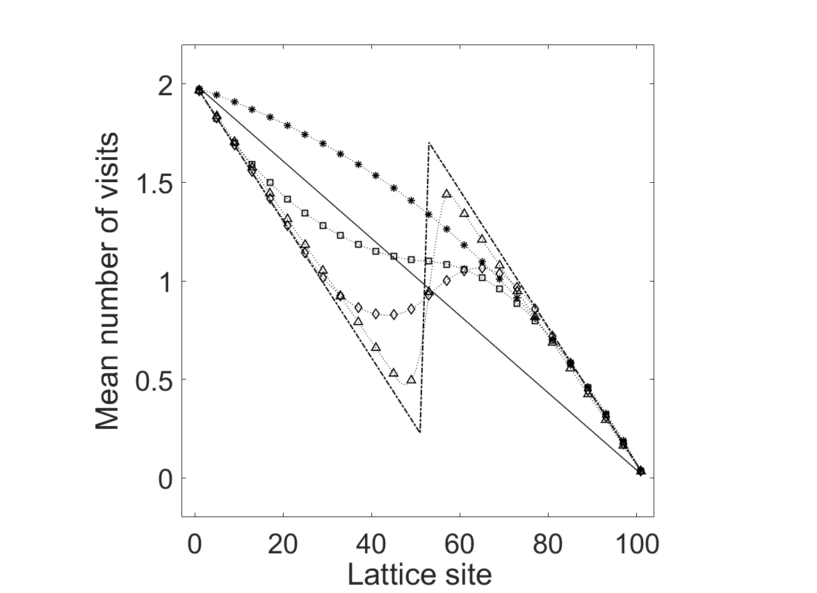
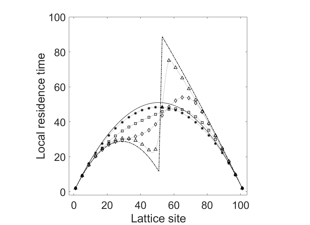
In Fig. 4.5 the effect of the motion of the defect in terms of mean number of visits and local residence times is reported, comparing the model with fixed and static defect with Models C and D. The mean number of visits and local residence times corresponding to the fixed and static defect model and to Model C have been computed through formulae (3.23), (3.25), (3.28) and (3.30) respectively. The profiles for Model D have been obtained through the general formulae (2.15) and (2.4) where (2.21) has been used for the right-exit probability.

In this case, the main effect of the defect motion on the mean number of visits and on the local residence times is to smooth out the profiles and produce a transition from the discontinuous piecewise-linear behavior of the model with fixed defect to the continuous, smooth profile related to Model C, where the defect can be found uniformly at random in every site of the lattice. In particular, taken Model D, the case $a=0$ ideally coincides with the model with fixed defect, since the defect has probability $1$ to be placed in a specific site.

Figure 4.6: Residence times for Model D as functions of $a/L$. From the left to the right, Model D with mode $d=25,\>51,\>75$. In all the panels $L=101$ and empty circles, triangles and diamonds refer to defect intensities of $\epsilon=0.2,\>0.3,\>0.4$ respectively. The solid horizontal lines correspond to residence times in the model with fixed and static defect, namely $\Gamma=5167.5,\>4565.4,\>4110.3$ time steps for $d=25$ and $\epsilon=0.2,\>0.3,\>0.4$ respectively, $\Gamma=3467.7$ time steps for $d=51$ and $\Gamma=3035.8,\>2868.9,\>2725.5$ time steps for $d=75$ and $\epsilon=0.2,\>0.3,\>0.4$ respectively. Asterisks in central panel indicate the residence times obtained from simulations.

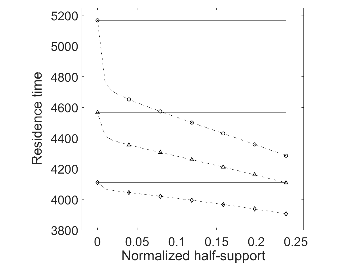
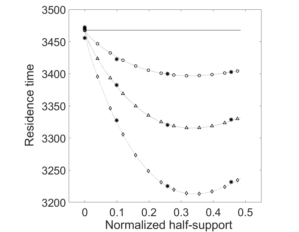
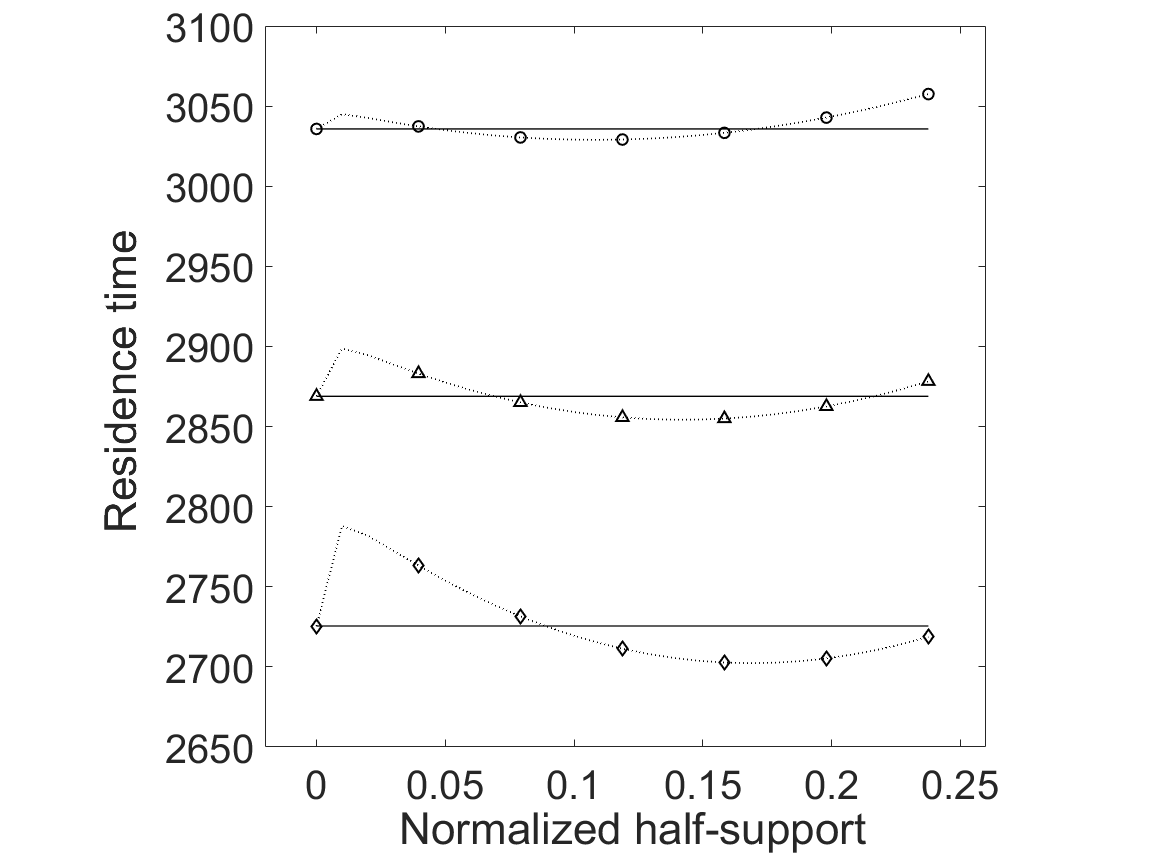
A noticeable aspect is the effect of the defect motion on the residence time $\Gamma$. It can be observed that, independently of the value of $\epsilon$ (with $\epsilon>0$) and from the width of the triangular distribution (parameterized by the width normalized to the lattice length, namely $a/L$), the residence time in presence of a moving defect is always shorter than that of the system with fixed defect, at least when the center $d$ of the distribution coincides with the central lattice site or it is placed at its left, see left and central panels in Fig. 4.6. When $\epsilon>0$ and the center of the distribution is placed in the right half of the lattice, there is only a finite interval of values of $a/L$ for which the residence time in presence of the moving defect is shorter than the corresponding for the fixed defect, as can be seen from the right panel in Fig. 4.6.

The most important observation about this model is the residence time invariance with respect to the sign of $\epsilon$ when $\Gamma$ is a function of the defect motion (to be intended as the triangular distribution spread $a$). In fact, the behavior of $\Gamma$ shown in Fig. 4.6 is also obtained for $\epsilon<0$, except for the fact that the behavior observed for $d=25$ in the case $\epsilon>0$ is recovered for $d=75$ and $\epsilon<0$ and vice-versa. This symmetry with respect to the central site of the lattice for different signs of $\epsilon$ is of the same nature of that shown in Fig. 3.1 and can be traced back to the effects of the hopping probabilities $p_{k}$ and $q_{k}$ on formulae (2.15), (2.16) and (2.21). More specifically, this result can be explained as follows: defect moving around the central lattice site and having positive intensity will increase the local residence time in the sites to the right of the center and decrease it in those to the left; on the other hand, defect moving around the central lattice site and with negative intensity will have the opposite effect. In these two systems, the local residence times will be distributed differently (in particular, they will be symmetric with respect to the lattice center) but they will sum up to the same value of $\Gamma$.

These remarkable results on the behavior of such a system have been tested against computer simulations (see Fig. 4.6, central panel, for the residence times resulting from simulations). In particular, a random walk on the line algorithm has been implemented which takes into account the dynamics of the defect site. A large enough number ($15\cdot 10^{6}$) of walks have been simulated and averages over the resulting set of trajectories have been computed. As shown in the central panel of Fig. 4.6, an optimal agreement between simulations and theory is obtained for all the tested values of $\epsilon$ and $a$.

5 Discussion and conclusions

We have studied the residence time in the framework of a simple random walk on a 1D lattice that we called lane. By using the theory of absorbing Markov chains we have first derived the expression (2.5), in which the residence time is written in terms of the probability that the walker started at a generic site $i$ exits the lane through the right exit at $L$ and the mean number of visits that the walker pays at site $i$. For these building bricks we have found general expressions, in Sections 2.2 and 2.3, which are valid for any choice of the left an right jump probabilities, $q_{k}$ and $p_{k}$, defining the walk.

These results have then been used in Section 3 to write the residence time in the case of a homogeneous walk with a single static defect. In particular, in Sections 3.1 and 3.2, we have derived explicit expressions for the residence time in the symmetric and in the driven case. Those expressions revealed to be very useful in the following sections to study cases in which a defect dynamic is considered. In particular we have shown that adding a dynamic to the defects induces a smoothing of the observable behaviors that present abrupt jumps in the case of a static defect.

Although the simple random walk is a very basic model, we have seen how it can provide general interesting insights for the residence time behavior, such as the large $L$ behavior. One of the interesting features of studying simplified models is the fact that they can help to shed some light on the behavior of much more complex systems. We want to discuss two interesting cases coming from two very different applicative contexts.

We first consider the crowd dynamics problem introduced in the paper [23]: pedestrians move from the left to the right through a rectangular corridor avoiding other pedestrians which form vertical queues, namely, queues orthogonal with respect to the direction of motion of the passing pedestrians. The model introduced in this paper is very complicated, many parameters accounting for the several interaction acting on the pedestrians are considered, and it is used to study in detail the different effects that enter in the computation of the residence time, i.e., the mean time needed by the passing pedestrian to cross the corridor. In particular the authors compute the quantity $I_{\textrm{pas}}$, which is defined as the ratio between the residence time in absence of queues and the residence time in presence of queues. In particular, in [23, Fig. 8], the authors study its behavior as a function of the parameter $\phi$, which is the parameter weighting the repulsive force that the passing pedestrians exert on the queuing ones.

In our simplified modelling, the walker can be thought as the passing pedestrian and the effect of the queuing pedestrians on it can be reduced to the presence of the defect site. Our model can be thought as a sort of effective model for the passing pedestrian problem with the parameter $\epsilon$, associated with the defect, containing all the informations on the interactions conditioning the motion of the passing pedestrians. For instance, coming back to [23, Fig. 8], it is possible to use our explicit formula (3.31) for the residence time in the driven case to fit the data of [23, Fig. 8] assuming that the effective $\epsilon$ is related to the parameter $\phi$ by the very general function

$$\epsilon(\phi)=\bar{a}\frac{\phi^{\alpha}}{\phi^{\alpha}+c}-\bar{b}.$$ (5.32)

If we consider, in our model, $p=0.55$ and $q=0.45$, from the extreme data in the picture we have that $\bar{a}=0.2230$ and $\bar{b}=0.4152$. Performing the best fit we find $\alpha=6.043$ and $c=1.074$. The comparison between our prediction and the data in [23] is depicted in Fig.5.7.

Figure 5.7: Fitting of the values of the efficiency parameter $I_{\textrm{pas}}$ as extracted from [23, Fig. 8]. Dotted line with empty circles represents the data to be fitted, while the solid line is the analytical $I_{\textrm{pas}}$ as a function of $\epsilon(\phi)$ obtained by using formula (3.31) for the residence times and fitting the parameters in formula (5.32).

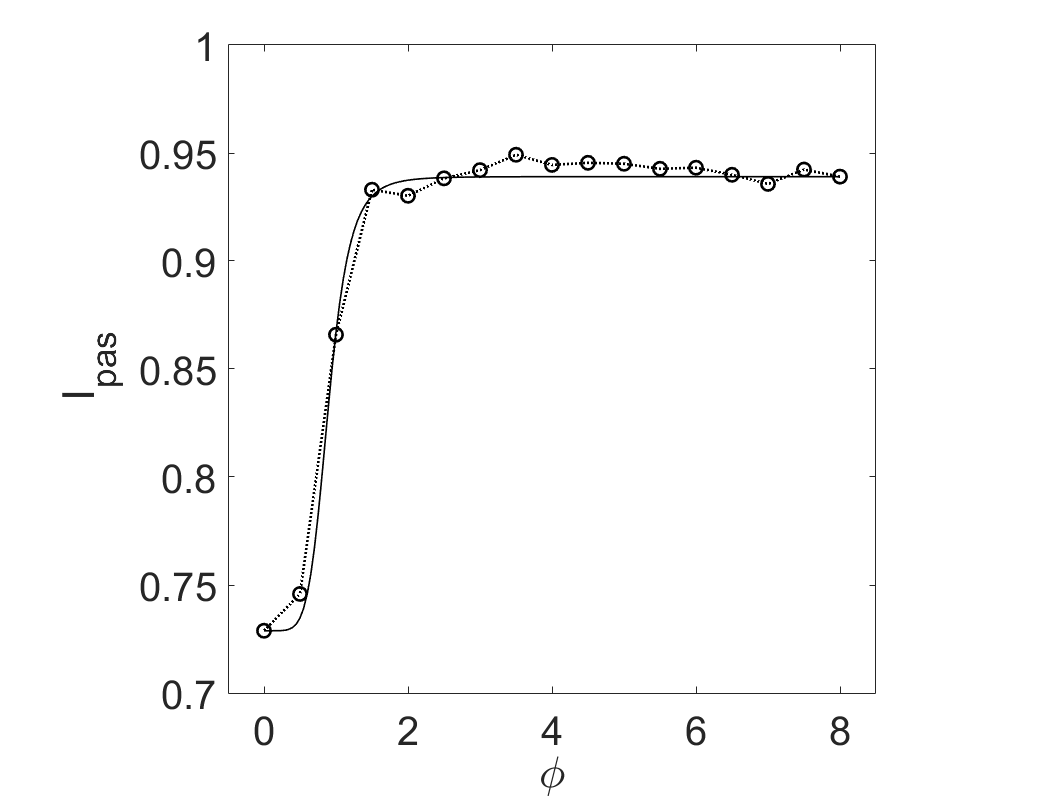
Equation (5.32) gives the effective value, as a function of the parameter $\phi$, of the decrease in probability that the passing pedestrian crosses the queue when it reaches it. It is worth nothing that this result is robust in the sense that the fitting parameters $\alpha$ and $c$ appear to depend poorly on the choice of the left and right jumping probabilities $p$ and $q$ in the simple random walk model.

Another relevant application of the residence time idea is related to stormwater runoff ponds design. Water running off from residential and urban areas, possibly after severe meteorological events like storms and heavy rainfalls, is known to drain and transport lots of different pollutants, which may result in a serious threat for water or marine ecosystems. To prevent drained pollutants to reach delicate water ecosystems, natural and artificial ponds are used to accelerate the deposition and absorption of undesired substances and components. As it has been demonstrated [24], residence times of the water flow inside the ponds are of crucial impact on their effectiveness. In particular, the higher the residence time, the higher is the pond efficiency in terms of deposition of pollutants [25]. Different design strategies, aimed at increasing the efficacy of the ponds, have been proposed. For instance, the installation of baffles, underwater berms or surface islands, acting as obstacles to the water flow, can increase significantly the residence time [26, 27].

Design aspects, like the maximization of the residence time, are studied in the literature by means of fluidodynamic approaches [26]. It is very interesting to remark that the qualitative behavior of those results can be interpreted by using our random walk model. We analyze, for instance, the results discussed in [26] where a rectangular pond is considered and the water inlet and outlet are placed symmetrically on the shortest sides of the pond. In particular we focus on the results reported in [26, Fig. 5], where RTD curves are plotted versus time in five cases: pond with no baffle (case 1), pond with an island placed at one quarter of pond length from the inlet (case 5), pond with an island placed at one tenth of pond length from the inlet (case 6), pond with a subsurface bern placed at one quarter of pond length from the inlet (case 7), pond with a subsurface bern placed at half pond length from the inlet (case 8). Those curves have been found by solving numerically suitable fluidodynamic equations.

These geometries are compatible with our 1D model, since the islands and the berns act symmetrically along the direction parallel to the shortest sides of the pond, namely, the direction orthogonal to the main water motion.

Data in [26, Fig. 5] show that the residence time in case 5 is larger than that in case 6, which, on turn, is larger than the residence time in case 1. This is precisely what we observe in our random walk driven model discussed in Section 3.2. Indeed, if one focuses on any of the curves with larger drift plotted in the left panel of Fig. 3.2, one can see that the residence time increases when a defect is placed at the site $10$ (one tenth of the length of the lane) and increases even more when it is placed at the site $25$ (one fourth of the length of the lane).

Figure 5.8: Residence time as a function of $d$ for a uniformly driven random walk with $p=0.54$, $\epsilon=-0.3$ and $L=101$. Dotted line with plain squares refers to the residence time of the walker for varying defect site. Horizontal solid line corresponds to the residence time of the driven random walk with same value of $p$, but without defects. The no-defect residence time is $\Gamma=1119$ time steps, while for $d=10$ and $d=25$ the residence times are $\Gamma=1127,\>1274$ time steps respectively.

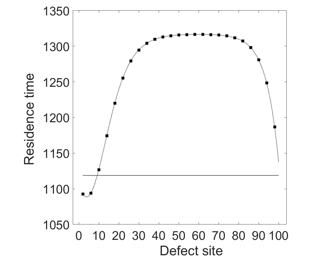
In particular, Fig. 5.8 shows the case in which $p=0.54$, where this behavior is more visible.

The random walk model does not appear to be completely effective when berns are considered. Indeed, data in [26, Fig. 5] show that the residence time in case 7 (very similar to the one measured in case 5) is larger than that in case 8, which, on turn, is larger than the residence time in case 1. The fact that the residence time in case 7 is larger than that in case 1 is compatible with our results plotted in the left panel of Fig. 3.2. On the other hand, based on our analysis, we would have expected that the residence time in case 8 would have been very similar to the one measured in case 7, but this seems not to be the case.

Summarizing, we have developed a rather complete theory of the residence time for the random walk in presence of defects. In particular, we have found explicit expressions in the case of a single defect, both in the symmetric and in the driven case. We have discussed our results in the framework of our abstract model and we have also shown how they can help, to some extent, to understand the behavior of much more complex systems.

Appendix A Analogy with the stationary occupation number profile

We consider a system of many independent particles performing a random walk on $1,\dots,L-1$ in continuous time. We suppose particles move with rate one according to the jump probabilities introduced in Section 2. Moreover, particles are introduced with rate $\alpha$ at site $1$ and $\delta$ at site $L-1$.

This system can be recast as a Zero Range Process with open boundaries and intensity function associated with site $i$ equal to the number of particles occupying such a site [28, 29].

The mean value of particles occupying each site of the lane $1,\dots,L-1$ at stationarity satisfy a set of recursive equation identical to equations (2.14) provided we choose $\alpha=1$ and $\delta=0$. See, for instance, [30, equation (13)], where the equations are reported for a case in which the jump probabilites are spatially homogeneous, or [29, equation (14)], where the equations are again reported for a case in which the jump probabilites are spatially homogeneous but the presence of a defect site is taken into account. The generalization of the formulae in [30, 29] to the case of arbitrary jumping probabilities is straightforward.

Thus, we can conclude that the mean number of visits profile of a random walk with two absorbing site coincides with the stationary occupation number profile of the independent particles Zero Range Process with same jumping probabilities and inlet rate $1$ on the left–end of the lane and $0$ on the right–end of the lane.

In [29] the stationary occupation number profile has been explicitly computed in the symmetric case discussed here in Section 3.1 for the defect at the center of the lane. Indeed, equations (3.22) and (3.23) reduces to [29, equations (20) and (21)] provided we choose the parameters as follows: $L-1=2R+1$, $d=R+1$, $\alpha=1$, and $\delta=0$.

References

- [1] G. Lane-Serff, L. Beal, T. Hadfield, Gravity current flow over obstacles. Journal of Fluid Mechanics 292, 39 – 53, 1995.
- [2] C. H. K. Williamson, Vortex dynamics in the cylinder wake Annu. Rev. Fluid. Mech. 28, 477–539, 1996.
- [3] O. Chepizhko, T. Franosch, Ideal circle microswimmers in crowded media Soft Matter 15, 452–461, 2019.
- [4] M. J. Creed , S. Draper , T. Nishino and A. G. L. Borthwick, Flow through a very porous obstacle in a shallow channel Proc. R. Soc. A 473, 20160672, 2017.
- [5] J. P. Gleghorn, J. P. Smith, J. B. Kirby, Transport and collision dynamics in periodic asymmetric obstacle arrays: Rational design of microfluidic rare-cell immunocapture devices J. Phys. Rev. E 88, 032136, 2013.
- [6] H. Wang, P. Iovenitti, E. Harvey, S. Masood, Optimizing layout of obstacles for enhanced mixing in microchannels Smart Mater. Struct. 11, 662, 2002.
- [7] A. J. Ellery, R.E. Baker, S. W. McCue, M. J. Simpson, Modeling transport through an environment crowded by a mixture of obstacles of different shapes and sizes, Physica A: Stat. Mech. App. 449, 74 – 84. 2016.
- [8] A. D. Borba, J. L. C. Domingos, E. C. B. Moraes, F. Q. Potiguar, W. P. Ferreira, Controlling the transport of active matter in disordered lattices of asymmetrical obstacles Phys. Rev. E 101, 022601, 2020.
- [9] M. J. Saxton, Anomalous diffusion due to obstacles: a Monte Carlo study Biophysical Journal 66, 394–401, 1994.
- [10] H. Berry, H. Chaté, Anomalous diffusion due to hindering by mobile obstacles undergoing Brownian motion or Orstein-Ulhenbeck processes. Phys. Rev. E 89 (2), 022708, 2014.
- [11] T. Sentjabrskaja, E. Zaccarelli, C. De Michele, F. Sciortino, P. Tartaglia, T. Voigtmann, S. U. Egelhaaf, M. Laurati Anomalous dynamics of intruders in a crowded environment of mobile obstacles Nat Commun. 7, 11133, 2016.
- [12] T. Harayama, R. Klages, P. Gaspard, Deterministic diffusion in flower shape billiards Phys. Rev. E 66, 026211, 2002.
- [13] D. Andreucci, E.N.M. Cirillo, M. Colangeli, D. Gabrielli. Fick and Fokker–Planck diffusion law in inhomogeneous media. J. Stat. Phys. 174: 469–493, 2019.
- [14] E.N.M. Cirillo, M. Colangeli, Blockage-induced condensation controlled by a local reaction, Phys. Rev. E 94, 042116, 2016.
- [15] M. Menshikov, S. Popov, A. Wade, Non-homogeneous Random Walks: Lyapunov Function Methods for Near-Critical Stochastic Systems, Cambridge University Press, 2016.
- [16] J.G. Kemeney, J.L. Snell, Finite Markov chain, Springer–Verlag, 1960.
- [17] A. Ciallella, E.N.M. Cirillo, Conditional expectation of the duration of the classical gambler problem with defects European Physical Journal Special Topics 228 111-128, 2019
- [18] A. Ciallella, E.N.M. Cirillo, J. Sohier, Residence time of symmetric random walkers in a strip with large reflective obstacles, Physical Review E 97, 052116, 2018.
- [19] E.N.M. Cirillo, A. Ciallella, B. Vantaggi, Localization of defects via residence time measures, arXiv:2011.08624, 2020.
- [20] R.A. Usmani, Inversion of Jacobi’s Tridiagonal Matrix, Computers Math. Applic. 27, 59–66, 1994.
- [21] W. Feller, An Introduction to Probability Theory and its Applications, volume 1, John wiley & Sons, Inc, New York – London – Sidney, 1968.
- [22] J. Messelink, R. Rens, M. Vahabi, F.C. MacKintosh, A. Sharma, On-site residence time in a driven diffusive system: Violation and recovery of a mean-field description, Physical Review E 93, 01211, 2016.
- [23] P.–Y. Wu, R.–Y Guo, Simulation of pedestrian flows through queues: Effect of interaction and intersecting angle, Physica A 570, 125804, 2021.
- [24] D.J. Walker, Modelling residence time in stormwater ponds, Ecological Engineering 10, 247–262, 1998.
- [25] J. F. Holland, J. F. Martin, T. Granata, V. Bouchard, M. Quigley, L. C. Brown, Effects of wetland depth and flow rate on residence time distribution characteristics, Ecological Engineering 23, 189-203, 2004.
- [26] S. Khan, B. Melville, A.Y. Shamseldin, Modeling the layouts of stormwater retention ponds using residence time, 4th IASME/WSEAS International Conference on Water Resources, Hydraulics and Hydrology, 2009.
- [27] J.C. Agunwamba, Field pond performance and design evaluation using physical models, Water Research 26, 1403–1407, 1992.
- [28] M.R. Evans, T. Hanney, Nonequilibrium statistical mechanics of the zero–range process and related models, J. Phys. A: Math. Gen. 38, R195–R240, 2005.
- [29] E.N.M. Cirillo, M. Colangeli, Stationary uphill currents in locally perturbed Zero Range Processes, Phys. Rev. E 96, 052137, 2017.
- [30] E. Levine, D. Mukamel, G.M. Schütz, Zero–Range Process with Open Boundaries, J. Stat. Phys. 120, 759–778, 2005.