Combining Reward and Rank Signals for Slate Recommendation

Abstract.

We consider the problem of slate recommendation, where the recommender system presents a user with a collection or slate composed of $K$ recommended items at once. If the user finds the recommended items appealing then the user may click and the recommender system receives some feedback. Two pieces of information are available to the recommender system: was the slate clicked? (the reward), and if the slate was clicked, which item was clicked? (rank). In this paper, we formulate several Bayesian models that incorporate the reward signal (Reward model), the rank signal (Rank model), or both (Full model), for non-personalized slate recommendation. In our experiments, we analyze performance gains of the Full model and show that it achieves significantly lower error as the number of products in the catalog grows or as the slate size increases.

1. Introduction

Slate recommendation, also referred to as banner recommendation, is the task of recommending a collection of $K$ items at once to the user. This problem arises in many real-world applications like search and online advertising. The logs of the recommender system can be used to refine future recommendations by the use of two distinct signals. First, the reward signal that identifies slates that the user interacts with. For example, if we recommend to a user a slate of two items: phone and couscous, and the user interacts with that recommendation, then the slate receives a reward of $1$ (and perhaps the user finds the slate appealing as a whole). Second, the rank signal that describes which item was interacted with within the slate. For example, if we recommend to a user a phone and couscous, and the user clicks on the couscous, then the rank is 2 (the user interacted with the 2nd item, and perhaps prefers it to the first). The rank signal is an item-level information that gives an individual ranking characterizing the score of a click on an item in the slate. Non-personalized slate recommendation algorithm can either use the reward signal (the number of clicks & non-clicks on the slate), the rank signal (number of clicks on each item in a slate), or both to decide which slate to display to the users.

The following is an introductory example for this setting. We consider a catalog containing $3$ items: phone, couscous, and beer. Ignoring order, there are $3$ possible slates with size $2$ that we can recommend: [phone, couscous], [phone, beer] or [phone, couscous]. Using historical data summarizing the interactions with these three slates, we consider how to determine the best slate to display to the user. An example of historical data is given in Table 1, where we show each of the 3 slates 700 times. Here, slate [couscous, beer] is the best one. The most direct evidence for this is that it has the lowest number of non-clicks (626) and hence the highest click through rate ($1-\frac{626}{700}\approx 0.11$). There is also indirect evidence using click rank that couscous is preferred to phone (29 clicks vs. 10), beer is preferred to phone (47 clicks vs. 9), and couscous is preferred to beer (46 clicks vs. 28). In aggregate, this ranking information also suggests that [couscous, beer] is the best slate - this suggestion is conditional upon a modeling assumption that there are not virtuous or counterproductive combinations of items in slates - which we will make rigorous shortly.

Slate	non-clicks	clicks on 1	clicks on 2
phone, couscous	661	10	29
phone, beer	644	9	47
couscous, beer	626	46	28

Table 1. Example of slate recommendation historical data.

Bandit algorithms are actively being developed for online slate recommendation. In general, bandit algorithms are provably optimal and have strong theoretical guaranties. In the multi-armed bandits setting (Robbins, 1952; Slivkins, 2019; Lattimore and Szepesvári, 2020), algorithms rely on the reward signal only. It has been shown that their performance deteriorates in online slate recommendation as the number of possible slates is combinatorially large (Dimakopoulou et al., 2019; Rhuggenaath et al., 2020). In combinatorial bandits/semi-bandits settings, some studies assume access to the reward signal as a function, with certain properties , of the unknown items ranking (Cesa-Bianchi and Lugosi, 2012; Combes et al., 2015; Dimakopoulou et al., 2019), and others assume direct access to items ranking (Kale et al., 2010; Kveton et al., 2015; Qin et al., 2014; Wen et al., 2017).

In offline settings, numerous reward modeling approaches have been proposed in the context of slate recommendation. In (Swaminathan et al., 2017), off-policy evaluation and optimization procedures were developed which allow evaluation of new slate recommendation policies, as well finding the one that achieves maximal reward. In that study, reward signal is assumed to be additive w.r.t unknown items ranking. In (Jiang et al., 2019), authors assume access to items ranking, and use them to train conditional variational autoencoders that models items distribution and enables slates generation for recommendation.

In production, and perhaps surprisingly, practical algorithms often ignore the reward signal and rely on ranking items to learn user preferences. An example of such models is a simple extension of the Pop model in (Cremonesi et al., 2010), where the agent recommends a slate composed of the top $K$ most popular items. Other examples of relevant work include (Covington et al., 2016; Bello et al., 2019; Rendle et al., 2012). In our experience, the reward signal is often ignored in recommender systems since it is difficult to integrate it into the target cost function which is based on ranking items correctly. Another reason can be organisational - different teams in the company might focus either on the reward or on items ranking. Such separation is typical in online advertising - bidding team typically focuses on reward prediction, whereas recommendation team is only interested in ranking candidates correctly.

In this paper, we formulate three intuitive Bayesian models that use either the reward signal (Reward model), the rank signal (Rank model), or both (Full model). These algorithms learn from offline historical data similar to the example presented in Table 1, and allow consistent estimation of the underlying reward model. We demonstrate empirically that the Full model outperforms the other two approaches highlighting the benefits of combining both, the reward and rank signals.

2. Bayesian Formulation of Full, Reward & Rank Models

(a) Varying catalog size.

(b) Varying slate size.

(c) Varying N° of samples.

(d) Catalog with 20 items.

Figure 1. Figures (a, b ,c): $L_{1}$ error (Eq. 1) for varying slate size, catalog size, and number of times each slate appears in the data. In each experiment, we run the models 50 times and average the results. Shaded areas represent uncertainty. Figure (d): Violin plot of $L_{1}$ errors distribution. Here, we generate samples $\tilde{\theta}_{i}$ from the posterior and calculate the $L_{1}$ distance (Eq. 1) between vectors $p_{\theta}$ and $p_{\tilde{\theta}_{i}}$ for all samples $\tilde{\theta}_{i}$. This results in a set of $L_{1}$ errors that we visualize using the violin plot.

2.1. Setting

We consider non-personalized slate recommendation. Interaction between items in a slate is ignored, meaning that the best slate is the one composed of the overall best $K$ items. In addition, the order of items in a slate doesn’t matter, meaning that recommending [item1, item2] is the same as recommending [item2, item1]. The statistics of slate interaction with users is summarized in the following $K+1$ variables, the number of non-clicks on the slate $nc$, and the number of clicks on each item of the recommended slate of size $K$, which we denote $c_{i}$ for $i\in[K]$. Other useful variables, which can be derived from the ones defined previously, are the number of clicks on the recommended slate $c=\sum_{i\in[K]}c_{i}$, and the number of impressions $I=c+nc$. Table 3 in Appendix A summarizes the remaining variables as well as the ones we have already mentioned.

2.2. Bayesian Formulation & Learning

2.2.1. Formulation

We present three intuitive and simple Bayesian approaches that allow consistent estimation of the underlying reward model in non-personalized slate recommendation. We chose the Bayesian framework because it is highly flexible, since it allows us to incorporate prior information. In addition, it is suited to many MCMC sampling methods that allow consistent estimation of the posterior distribution of the parameters. We start by introducing two important parameters $\phi$ and $\theta$. $\phi$ is a real-valued random variable that quantifies the overall magnitude of a non-click on the slates (i.e. magnitude of the reward signal). A large value of $\phi$ means that users tend to not click on slates very often. $\theta=[\theta_{1},\dots,\theta_{N}],$ with $N$ as the catalog size is a random vector where each coordinate $\theta_{i}$ represents the score of a click on item $i$ in the catalog independently of the slate in which it appears.

The Full model makes use of both reward and rank signals. In this model, we put Gamma priors over the magnitude of a non-click on the slates $\phi$ and the scores of a click on each item in the catalog $\theta$. Conditioned on $\phi$, $\theta$, the recommended slate $a$, and the number of impressions $I$, we model the number of non-clicks $nc$ and the number of clicks on each item $c_{i},i\in[K]$ using a multinomial distribution with $K+2$ parameters $I,q,p_{1},\dots,p_{K}$ expressed as follows:

$$nc,c_{1},\dots,c_{K}|I,\phi,\theta,a\sim{\rm Multinomial}\left(I,q,p_{1},\dots,p_{K}\right),$$

with $q$ (probability of a non-click on the slate $a$) and $p_{i},i\in[K]$ (probability of a click on the $i$-th item of the slate $a$) are obtained by normalizing the scores $\phi$ and $\theta$ across slate $a$.

The Reward model ignores items ranking (number of clicks on each item in the slates), and only uses the reward signal (i.e. number of clicks on the slates). First, Gamma priors are put over $\phi$ and $\theta$. Conditioned on relevant random variables, we model the number of non-clicks on the slate $nc$ and the number of clicks on the slate $c$ by a multinomial distribution with parameters $I,q,p$:

$$nc,c|I,\phi,\theta,a,\sim{\rm Multinomial}\left(I,q,p\right),$$

with $q$ (probability of a non-click the slate $a$) and $p$ (probability of a click on the the slate $a$) are obtained by normalizing scores $\phi$ and $\theta$ across slate $a$.

The Rank model takes into account items ranking only (the number of clicks on each item in the slates). First, Gamma prior is put over the scores $\theta$. Conditioned on the number of clicks on the slate $I_{c}$ and other relevant random variables, we model the number of clicks on each item in the slate $c_{i}$ by a multinomial distribution with $K+1$ parameters $I_{c},p_{1},\dots,p_{K}$:

$$c_{1},\dots,c_{K}|I_{c},\theta,a\sim{\rm Multinomial}\left(I,p_{1},\dots,p_{K}\right),$$

with $p_{i},i\in[K]$ is the probability of a click on the $i$-th item in slate $a$, and is obtained by carefully normalizing scores $\theta$ across slate $a$.

We emphasize that three methods allow consistent estimation of parameter $\theta$, and both the Full and Reward models also allow consistent estimation of parameter $\phi$. In addition, note that the Rank and Full models are equivalent when $\phi=0$. Meaning that if the magnitude of the reward signal is always 0 (the slate is always clicked), then adding the reward signal to items ranking does not provide any additional information. On the other hand, if $\phi\rightarrow\infty$, then the reward signal becomes dominant, and items rankings would be irrelevant without it. In practice, $\phi$ is reasonably high, but not to the point that items ranking becomes irrelevant.

Table 2 shows these three models for slates with size 2. Here, we present how to derive parameters of the multinomial distribution for the Full model in that case. Conditioned on $I,\phi,\theta,a_{1},a_{2}$, with $a=[a_{1},a_{2}]$ as the recommended slate of size 2, variables $nc,c_{1},c_{2}$ are modeled by ${\rm Multinomial}\left(I,q,p_{1},p_{2}\right),$ with $q=\phi/(\phi+\theta_{a_{1}}+\theta_{a_{2}})$ is the probability of a non-click on the recommended slate $a$, $p_{1}=\theta_{a_{1}}/(\phi+\theta_{a_{1}}+\theta_{a_{2}})$ is the probability of a click on the first item $a_{1}$ and $p_{2}=\theta_{a_{2}}/(\phi+\theta_{a_{1}}+\theta_{a_{2}})$ as the probability of a click on the second item $a_{2}$. One can follow the same reasoning to derive the probabilities of the Multinomial distributions for the other two models in Table 2, or for an arbitrary slate size.

Model Description Full $nc,c_{1},c_{2}|I,\phi,\theta,a_{1},a_{2}\sim{\rm M}\left(I,\frac{\phi}{\phi+\theta_{a_{1}}+\theta_{a_{2}}},\frac{\theta_{a_{1}}}{\phi+\theta_{a_{1}}+\theta_{a_{2}}},\frac{\theta_{a_{2}}}{\phi+\theta_{a_{1}}+\theta_{a_{2}}}\right)$ Reward $nc,c|I,\phi,\theta,a_{1},a_{2}\sim{\rm M}\left(I,\frac{\phi}{\phi+\theta_{a_{1}}+\theta_{a_{2}}},\frac{\theta_{a_{1}}+\theta_{a_{2}}}{\phi+\theta_{a_{1}}+\theta_{a_{2}}}\right)$ Rank $c_{1},c_{2}|I_{c},\theta,a_{1},a_{2}\sim{\rm M}\left(I_{c},\frac{\theta_{a_{1}}}{\theta_{a_{1}}+\theta_{a_{2}}},\frac{\theta_{a_{2}}}{\theta_{a_{1}}+\theta_{a_{2}}}\right)$

Table 2. Models formulation for slates with size 2.

2.2.2. Learning

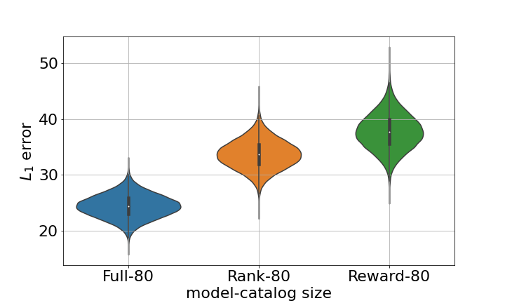
We assume access to historical data $\mathcal{D}$ of the form [slate $a$, non-clicks on $a$, clicks on $a_{1}$, $\dots$, clicks on $a_{K}$] (e.g. Table 1). Our representation of data $\mathcal{D}$ changes depending on the model we are using. The Full model takes data in its raw form. The Reward model transforms it into [slate $a$, non-clicks on $a$, clicks on $a_{1}+\dots+$ clicks on $a_{K}$] to take into account the reward signal only. In the Rank model, data is represented as follows [slate $a$, clicks on $a_{1}$, …, clicks on $a_{K}$], taking into account items ranking only. Parameters $\phi$ and $\theta$ are inferred via Maximum A Posteriori - MAP. For instance, with data $\mathcal{D}$, MAP estimators of $\theta$ and $\phi$ are obtained by maximising the posterior $p(\theta,\phi|\mathcal{D})$. Note that, in the case of Rank model, we only estimate $\theta$ since $\phi$ is ignored in that model. MAP was used to estimate parameters in all experiments, except violin plots where we used MCMC methods in Stan (Carpenter et al., 2017) to generate a set of samples $\tilde{\theta}_{i}$ from the posterior.

3. Experiments

3.1. Experimental Setup

We use synthetic data to compare our three methods. We generate $n$ samples of user interactions with each slate, using a multinomial distribution with known parameters $\phi=100$ and $\theta$ containing values evenly spaced from 1 to 6. This generative process leads to a dataset similar to the one presented in Table 1 and Section 2.2.2. We then fit our models to this data, and evaluate the ability of each model to estimate the true parameters of the generative process. Since all of our models estimate the parameter $\theta$, we use this parameter to evaluate the performance of all models. More precisely, we compute the $L_{1}$ distance between $p_{\hat{\theta}}$ (the vector of estimated probabilities of a click on item $1$ in each recommended slate $a$) and $p_{\theta}$ (the vector of true probabilities of a click on item $1$ in each recommended slate $a$).

(1) $$L_{1}(p_{\hat{\theta}},p_{\theta})=\sum\limits_{\text{all slates }a}\left|\frac{\hat{\theta}_{a_{1}}}{\sum_{j\in[K]}\hat{\theta}_{a_{j}}}-\frac{\theta_{a_{1}}}{\sum_{j\in[K]}\theta_{a_{j}}}\right|$$

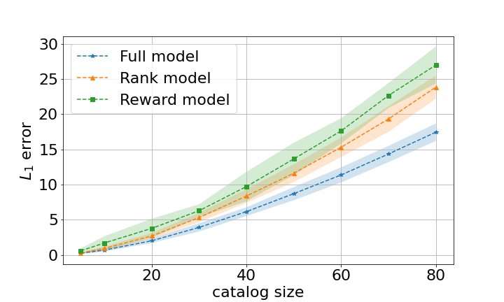
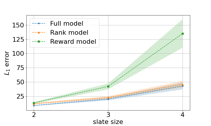
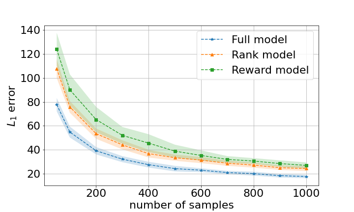
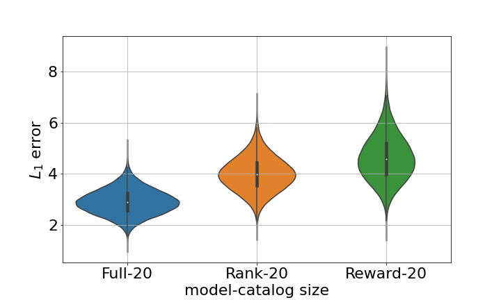
For experiments with varying slate and catalog sizes, the number of samples per slate $n$ is fixed and set to $1000$ (i.e. each slate appears $1000$ times in the data). We set the slate size to 2 for experiments with varying number of samples and varying catalog sizes. Catalog size is set to 50 for experiments with varying slate size. In Figures 1(a), 1(b), 1(c), we run all models 50 times, and report the empirical mean and standard deviation of $L_{1}$ errors over these 50 runs. In violin plots 1(d) and 3 in Appendix C, we use Stan to generate a set of samples $\tilde{\theta}_{i}$ from the posterior distribution. Eq. 1 is then used to calculate $L_{1}$ distance between $p_{\theta}$ and $p_{\tilde{\theta}_{i}}$ for all generated samples $\tilde{\theta}_{i}$. This process leads to a set of $L_{1}$ errors that we visualize with violin plots. Table 4 in Appendix B summarizes the parameters of all these experiments. As an additional experiment, we compare Full and Reward models ability to estimate the probability of a non-click on the slates. Precisely, we compare Full and Reward models using the $L_{1}$ distance between $\hat{q}$ (the vector of estimated probabilities of a non-click for all recommended slates $a$) and $q$ (the vector of true probabilities of a non-click for all recommended slates $a$).

(2) $$L_{1}(\hat{q},q)=\sum\limits_{\text{all slates }a}\left|\frac{\hat{\phi}}{\hat{\phi}+\sum_{j\in[K]}\hat{\theta}_{a_{j}}}-\frac{\phi}{\phi+\sum_{j\in[K]}\theta_{a_{j}}}\right|$$

Clearly, Rank model isn’t involved in this comparison as it doesn’t estimate the magnitude of a non-click $\phi$. Table 7 in Appendix D shows the results for this experiment.

3.2. Results

Figure 1 shows the results for our three models, with varying catalog sizes, slate sizes, and number of samples. In particular, the Full model achieves better $L_{1}$ error when the catalog size increases (Figure 1(a)). For instance, with 80 items in the catalog, the Reward and Rank models have $54\%$ and $36\%$ higher relative $L_{1}$ error than the Full model. In real-world settings, with partners having millions of items in their catalogs, the gap between the Full model and the two other models can become significant. Results for a catalog of size $50$ and different slate sizes are shown in Figure 1(b). The gap in performance between the Full and Rank models does not change when slate size increases, while the $L_{1}$ error for the Reward model grows at a much higher rate when the slate size increases. Recall that we have $n$ samples per slate in our data. Since the Reward model only exploits the reward signal, it only uses $n$ samples to estimate items scores, independently of the slate size. In contrast, the other two models use individual ranking. Therefore, the number of samples used to estimate items scores increases as the slate size increases. For instance, a single item would appear in many slates, meaning that samples from all of these slates will be used to estimate that item’s score. Figure 1(c) shows that the Full model outperforms the other two models for any number of samples. Additionally, we see that the gap in performance between models in Figure 1(c) seems to be constant. Figure 1(d) shows a violin plot of the $L_{1}$ errors obtained by sampling from the posterior for a catalog with 20 items. From Figure 1(d) we see that the $L_{1}$ error is more concentrated on the mean in the Full model compared to the Rank and Reward models. We invite the reader to see Tables 5, 6 in Appendix C for additional numerical results from our experiments.

4. Conclusion

In this paper we have formulated and compared Bayesian models for non-personalized slate recommendation. We have confirmed that the Full model, which utilizes both types of signals, reward and rank, is more favorable than any of the models that are based only on one type of signal. As such, we verified that as the catalog or slate size grows, the performance gains provided by the Full model increase as well.

The impact of the reward signal on the ranking quality demonstrated in this paper is of interest for industrial recommender systems. Although all three models provide an estimate of items scores, the difference between models in practice can be significant since the catalog for applications such as online advertising can contain hundreds of millions of items, and the error grows with the catalog size. A typical industrial personalized recommendation system is based on collaborative filtering and does not have room for including both types of signals considered in this paper. It usually favors the ranking signal over the reward one and is optimized for ranking items correctly on the training dataset. The Full model has the benefit of combining both signals and is optimized for predicting the actual outcome of the user interaction with the slate.

For future work, we plan to extend this framework to the personalized slate recommendation scenario, where the results of recommendations depend on user features. We also plan to test our framework on real-world slate recommendation datasets.

Appendix A Summary of Notations & Definitions

Following table summarizes definitions and notations of quantities used in the paper.

Notation Definition $N$ Catalog size. $I$ Total number of impressions. $I_{c}$ Total number of clicks. $K$ Slate size. $a=[a_{1},\dots,a_{K}]$ Recommended slate. $nc$ Number of non-clicks on a recommended slate $a$. $c$ Number of clicks on a recommended slate $a$. $\phi$ Score of a non-click. $\theta_{i},i\in[N]$ Scores of a click on item $i$. $c_{i},i\in[K]$ Number of clicks on the $i$-th item in the recommended slate $a$.

Table 3. Notations and Definitions

Appendix B Experimental setting details.

Following table provides details about all parameters used in our experiments.

Figure	slate size	catalog size	N° samples
1(a)	2	varying	1000
1(b)	varying	50	1000
1(c)	2	80	varying
1(d)	2	20	1000
3	2	80	1000

Table 4. Parameters values for different experiments.

Appendix C Experimental results.

	catalog size
Model	5	10	20	30	40	50	60	70	80
Full	0.23	0.69	2.02	3.91	6.15	8.71	11.36	14.34	17.44
Rank	0.28	0.94	2.70	5.31	8.37	11.60	15.29	19.31	23.83
Reward	0.59	1.70	3.77	6.28	9.72	13.64	17.62	22.64	26.97

	slate size
Model	2	3	4
Full	8.48	19.88	42.93
Rank	11.73	22.61	45.88
Reward	13.21	42.07	134.97

Table 5. $L_{1}$ errors for varying catalog size and slate size.

	number of samples
Model	5	10	50	100	200	300	400	500	600	700	800	900	1000	5000	10000
Full	250.69	171.30	77.67	54.77	39.15	32.11	27.48	24.20	22.87	20.90	19.98	18.32	17.59	7.85	5.50
Rank	360.00	241.73	107.76	75.80	53.42	44.08	36.72	33.32	31.32	28.72	27.14	24.96	24.27	10.65	7.45
Reward	419.56	287.23	124.00	90.08	65.22	52.00	45.49	38.83	35.20	31.89	30.54	28.40	26.90	12.18	8.49

Table 6. $L_{1}$ errors for varying number of samples.

Figure 3 is a violin plot for a catalog with 80 items.

Figure 2. Catalog with 80 items.

Figure 3. Violin plot of $L_{1}$ errors distributions for a catalog with 80 items. In this plot, we generate samples $\tilde{\theta}_{i}$ from the posterior and calculate the $L_{1}$ distance (Eq. 1) between vectors $p_{\theta}$ and $p_{\tilde{\theta}_{i}}$ for all samples $\tilde{\theta}_{i}$. This process results in a set of $L_{1}$ errors that we visualize using the violin plot.

Tables 5 and 6 show the results used in Figures 1(b), 1(a), 1(c).

Appendix D Additional Experiment

Table 7 shows the results for the additional experiment.

catalog size Model 5 10 20 30 40 50 60 70 80 Full 0.03 0.09 0.25 0.48 0.77 1.08 1.42 1.78 2.14 Reward 0.05 0.14 0.39 0.67 1.07 1.52 1.99 2.55 3.05

Table 7. $L_{1}$ errors (Eq. 2) for varying catalog size.

References

- (1)
- Bello et al. (2019) Irwan Bello, Sayali Kulkarni, Sagar Jain, Craig Boutilier, Ed Chi, Elad Eban, Xiyang Luo, Alan Mackey, and Ofer Meshi. 2019. Seq2Slate: Re-ranking and Slate Optimization with RNNs. arXiv:1810.02019 [cs.IR]
- Carpenter et al. (2017) Bob Carpenter, Andrew Gelman, Matthew D. Hoffman, Daniel Lee, Ben Goodrich, Michael Betancourt, Marcus Brubaker, Jiqiang Guo, Peter Li, and Allen Riddell. 2017. Stan: A Probabilistic Programming Language. Journal of Statistical Software, Articles 76, 1 (2017), 1–32. https://doi.org/10.18637/jss.v076.i01
- Cesa-Bianchi and Lugosi (2012) Nicolò Cesa-Bianchi and GáBor Lugosi. 2012. Combinatorial Bandits. J. Comput. Syst. Sci. 78, 5 (Sept. 2012), 1404–1422. https://doi.org/10.1016/j.jcss.2012.01.001
- Combes et al. (2015) Richard Combes, Mohammad Sadegh Talebi Mazraeh Shahi, Alexandre Proutiere, and marc lelarge. 2015. Combinatorial Bandits Revisited. In Advances in Neural Information Processing Systems, C. Cortes, N. Lawrence, D. Lee, M. Sugiyama, and R. Garnett (Eds.), Vol. 28. Curran Associates, Inc. https://proceedings.neurips.cc/paper/2015/file/0ce2ffd21fc958d9ef0ee9ba5336e357-Paper.pdf
- Covington et al. (2016) Paul Covington, Jay Adams, and Emre Sargin. 2016. Deep Neural Networks for YouTube Recommendations. In Proceedings of the 10th ACM Conference on Recommender Systems (Boston, Massachusetts, USA) (RecSys ’16). Association for Computing Machinery, New York, NY, USA, 191–198. https://doi.org/10.1145/2959100.2959190
- Cremonesi et al. (2010) Paolo Cremonesi, Yehuda Koren, and Roberto Turrin. 2010. Performance of recommender algorithms on top-N recommendation tasks. RecSys’10 - Proceedings of the 4th ACM Conference on Recommender Systems, 39–46. https://doi.org/10.1145/1864708.1864721
- Dimakopoulou et al. (2019) Maria Dimakopoulou, Nikos Vlassis, and Tony Jebara. 2019. Marginal Posterior Sampling for Slate Bandits. In Proceedings of the Twenty-Eighth International Joint Conference on Artificial Intelligence, IJCAI-19. International Joint Conferences on Artificial Intelligence Organization, 2223–2229. https://doi.org/10.24963/ijcai.2019/308
- Jiang et al. (2019) Ray Jiang, Sven Gowal, Timothy A. Mann, and Danilo J. Rezende. 2019. Beyond Greedy Ranking: Slate Optimization via List-CVAE. arXiv:1803.01682 [stat.ML]
- Kale et al. (2010) Satyen Kale, Lev Reyzin, and Robert E. Schapire. 2010. Non-Stochastic Bandit Slate Problems. In Proceedings of the 23rd International Conference on Neural Information Processing Systems - Volume 1 (Vancouver, British Columbia, Canada) (NIPS’10). Curran Associates Inc., Red Hook, NY, USA, 1054–1062.
- Kveton et al. (2015) Branislav Kveton, Zheng Wen, Azin Ashkan, and Csaba Szepesvari. 2015. Tight Regret Bounds for Stochastic Combinatorial Semi-Bandits. arXiv:1410.0949 [cs.LG]
- Lattimore and Szepesvári (2020) Tor Lattimore and Csaba Szepesvári. 2020. Bandit Algorithms. Cambridge University Press. https://doi.org/10.1017/9781108571401
- Qin et al. (2014) Lijing Qin, Shouyuan Chen, and Xiaoyan Zhu. 2014. Contextual Combinatorial Bandit and its Application on Diversified Online Recommendation. 461–469. https://doi.org/10.1137/1.9781611973440.53
- Rendle et al. (2012) Steffen Rendle, Christoph Freudenthaler, Zeno Gantner, and Lars Schmidt-Thieme. 2012. BPR: Bayesian Personalized Ranking from Implicit Feedback. arXiv:1205.2618 [cs.IR]
- Rhuggenaath et al. (2020) Jason Rhuggenaath, Alp Akcay, Yingqian Zhang, and Uzay Kaymak. 2020. Algorithms for slate bandits with non-separable reward functions. arXiv:2004.09957 [stat.ML]
- Robbins (1952) Herbert Robbins. 1952. Some aspects of the sequential design of experiments. Bull. Amer. Math. Soc. 58, 5 (1952), 527 – 535. https://doi.org/bams/1183517370
- Slivkins (2019) Aleksandrs Slivkins. 2019. Introduction to Multi-Armed Bandits. arXiv:1904.07272 [cs.LG]
- Swaminathan et al. (2017) Adith Swaminathan, Akshay Krishnamurthy, Alekh Agarwal, Miroslav Dudík, John Langford, Damien Jose, and Imed Zitouni. 2017. Off-policy evaluation for slate recommendation. arXiv:1605.04812 [cs.LG]
- Wen et al. (2017) Zheng Wen, Branislav Kveton, and Azin Ashkan. 2017. Efficient Learning in Large-Scale Combinatorial Semi-Bandits. arXiv:1406.7443 [cs.LG]