Gravitational Radiation from Accelerating Jets

Abstract

Non-spherical rapid acceleration of mass (or energy) to a relativistic velocity is a natural source of gravitational radiation. Such conditions arise in both long and short gamma-ray bursts whose central engine ejects relativistic jets. The resulting gravitational wave signal is of a memory type, rising to a finite level (of order $4G{\cal E}/r$) over a duration that corresponds to the longer of either the injection time and the acceleration time of the jet. We explore the properties of such signals and their potential detectability. Unfortunately, the expected signals are below the frequency band of Advanced LIGO-Virgo-Kagra, and above LISA. However, they fall within the range of the planned BBO and DECIGO. While current sensitivity is marginal for the detection of jet gravitational wave signals from GRBs, hidden relativistic jets that exist within some core collapse SNe could be detected. Such a detection would reveal the acceleration mechanism and the activity of the central engine, which cannot be explored directly in any other way.

I Introduction

Gamma-ray bursts (GRBs) are extremely energetic, with typical energies of ${\cal E}=10^{51}$ erg. Jets associated with a GRB are accelerated to high Lorentz factors, with ${\Gamma\gtrsim 100}$ being a typical value. They are highly anisotropic, with the ejected material being confined to a cone with opening angle ${\theta_{\rm j}\lesssim 10^{o}}$. These jets are accelerated from rest within a short time, and they last for fraction of a second (in short GRBs) to tens of seconds (in long ones). The acceleration of a relativistic jet produces a memory-type gravitational wave (GW) signal [1, 2]. Observations of this GW signal will reveal the nature of the jets and the acceleration process. Additionally, there is ample evidence for hidden jets activity within some supernovae [3, 4, 5, 6, 7, 6, 7, 8, 9]. The existence of these jets can be inferred only indirectly. A detection of this kind of GW signal is possibly the only direct way to identify these invisible jets and learn about their hidden features.

While the GW amplitude estimates [2, 10, 11], that are of order $10^{-24}-10^{-25}$ for reasonably nearby GRBs, and the relevant frequencies (that are in the decihertz range) both make detection difficult, it is worthwhile to get back to this problem, and explore in greater details both the characteristics and the detection prospects of the GW signal.

Segalis and Ori [1] and Piran [2] considered an instantaneously accelerated point particle, using the zero-frequency limit (ZFL). This approximation that corresponds to infinite acceleration is appropriate for describing the final jump in the amplitude of the GW. However, this approximation misses, naturally, the details of the temporal structure that are crucial for consideration of detection feasibility.

Sago et al. [10] generalized this result for a GRB model based on a large number of thin jets (“minijets”) [12] that are ejected at random angles within a cone and random times within the duration of the GRB. Within this model each minijet produces a single pulse and these pulses combine to form the GRB light curve. In their model each minijet is described by an instantaneously accelerated point particle generating a step function signal. The superposition of the different step functions results in a complicated GW light curve. The model captures the effects of the angular structure and of the overall duration of the GRB resulting in a typical time scale for the pulse rise time that is comparable to the duration of the burst.

Birnholtz and Piran [11] relaxed the instanteneous acceleration approximation and developed a scheme for calculating the GW signal from a continuously accelerating axisymmetric jet. The considered, following the fireball model [13], an acceleration model in which the jet’s Lorentz factor increases linearly with time (or distance) until it reaches its final value. They considered different angular structures and observers at different viewing angles taking into account integration over equal arrival time surfaces. The combined effects of prolonged acceleration and taking into account the integration over the arrival time surface results in a temporal structure of the order of the acceleration time at viewing angles close to the jet and longer at larger angles.

In this work, we calculate the GW emission from accelerating jetc combining both effects of prolonged acceleration and prolonged duration of ejection of the jet. We calculate properties of the GW that are universal and independent of particular acceleration models, and combine them with a realistic possible model of the ejection of outflow in GRBs to derive typical amplitudes and detection expectation of GRBs and other astrophysical jets. In the following we will be using G=c=1, but at times we introduce these coefficients for clarity.

The structure of the paper is as follows. We outline in §II the general description of the problem and following the methods of [11] (that consider instantaneous injection) and some results of [10] (that consider instantaneous acceleration) we describe the GW signals from systems with instantaneous ejection or instantaneous acceleration. We explore in §III the temporal structure focusing on the interplay between the two time scales that exist in the system, the acceleration time scale, $t_{\rm acc}$, and the overall duration of the activity of the central engine that accelerates the jet, $t_{\rm inj}$. We consider in §IV an example in use the temporal structure of GRBs’ light curves as a proxy for the activity of the central engine. Following this example we consider in §V the detectability of these signals and we summarize and discuss our results in VI.

II Instantaneous Ejection and Acceleration

We consider an idealized jet that is accelerated to an ultra-relativistic velocity. The jet has energy ${\cal E}=m\Gamma$, with $m$ the jet’s mass and $\Gamma$ its final Lorentz factor. To simplify the discussion we keep only the essential features of the problem (see Fig. 1). The jet is an axisymmetric top hat with an opening angle $\theta_{\rm j}$. The jet moves radially outwards, and every particle emitted at the same time accelerates in the same manner. Particles emitted at the same time maintain the shape of a radially expanding infinitesimally thin spherical cap. The observer is located at a distance $r$ and at an angle $\theta_{\rm v}$, relative to the jet’s symmetry axis.

The energy (or mass) ejection function, $\dot{m}(t)$, describes the rate of mass ejection, where $t$ is measured in the rest frame of the central engine, and is the same in the observer’s rest frame. The function $\dot{m}(t)$ is characterized by the timescale $t_{\rm inj}$. The acceleration is described by the function $\Gamma(t)$, where $t$ is measured in the central engine’s frame of reference. $\Gamma(t)$ is characterized by the acceleration timescale $t_{\rm acc}$. The time of flight scale that characterizes the arrival time from different angular regions of the jet is related to the acceleration time as

$$\tilde{t}_{\rm o}(\theta_{\rm v})=(1-\beta\cos\Delta\theta_{\rm v})t_{\rm acc},$$ (1)

where $\Delta\theta_{\rm v}$ is the “relevant” (as discussed later) angle between the observer and the source and $\beta$ is the jet’s velocity. As the critical time scale is the longer of the two we denote $t_{\rm c}\equiv{\rm max}(\tilde{t}_{\rm o},t_{\rm inj})$. As $\tilde{t}_{\rm o}$ depends on the viewing angle, the dominant time scale may be $t_{\rm inj}$ for some observers and $t_{\rm acc}$ for others.

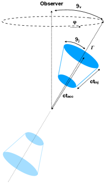
Figure 1: A schematic description of the jet. The top shell has reached the final Lorentz factor at a distance $ct_{\rm acc}$ from the origin. The duration of mass injection is $t_{\rm inj}$. A counter-jet is shown in light colors.

Among the different approximations, the zero-frequency limit (ZFL) stands out [1, 2]. This approximation ignores the detailed temporal structure of the source and the corresponding GW signal. The acceleration and mass ejection are instantaneous: $t_{\rm acc}=0$, and $t_{\rm inj}=0$. While non-physical, this limit gives an idea of the emerging patterns. It is also relevant for low-frequency detectors whose response is slower than the relevant timescales of the system. The waveform, in this limit, is described by a Heaviside step function:

$$h(t,\theta_{\rm v})=h_{0}(\theta_{\rm v})\mathcal{H}(t)\$$ (2)

and its Fourier transform is given by

$$\tilde{h}(f,\theta_{\rm v})={h_{0}(\theta_{\rm v})}/{f}\ .$$ (3)

II.1 A Point Particle - $\theta_{\rm j}=0$ and $t_{\rm inj}=0$

We begin considering a point particle of mass $m$ that is instantaneously accelerated to a Lorentz factor $\Gamma$ so that the total energy is ${\cal E}=m\Gamma$. The particle is moving at polar angles $\theta_{\rm v}$ and $\phi$ in the observer’s frame of reference (see Fig. 1). The gravitational wave amplitudes $h_{\rm+}$ and $h_{\rm x}$ of the two polarization modes are given by [1]:

$$h^{TT}(\theta_{\rm v})=h_{\rm+}+ih_{\rm x}=\frac{2{\cal E}\beta^{2}}{r}\frac{\sin^{2}\theta_{\rm v}}{1-\beta\cos\theta_{\rm v}}e^{2i\phi}.$$ (4)

For a single point-particle, the phase, $2i\phi$, can be ignored. When discussing the metric perturbation of an ensemble of particles, though, the complex phase may lead to destructive interference, and one component of the perturbation tensor may dominate over the other.

The angular dependence of the amplitude $h(\theta_{\rm v})$ exhibits anti-beaming: the GW amplitude vanishes along its direction of motion, and remains small at a cone around it. It reaches 50% of the maximal values at an opening angle $\Gamma^{-1}$. The function $h(\theta_{\rm v})$ attains a maximum of

$$h_{\rm max}=\frac{4{{\cal E}}}{r},\ \ \ \ {\rm at}\ \ \ \theta_{\rm max}=\sqrt{{2}/{\Gamma}}\ .$$ (5)

The total GW energy emitted is given by:

$$E_{\rm GW}=\frac{1}{32\pi}\iint{\dot{h}}^{2}dtd\Omega\ ,$$ (6)

where $\dot{\ }$ denotes time derivative. For an instantaneously accelerating particle, this integral diverges. However, this divergence is not physical, and it arises from the instantaneous approximation. For a finite acceleration time $t_{\rm acc}$ or a finite injection time the temporal integral can be calculated in Fourier space:

$$E_{\rm GW}=\frac{1}{32\pi}\int d\Omega\int_{0}^{f(\theta_{\rm v})}\tilde{h}(f)^{2}f^{2}df\ ,$$ (7)

where $f(\theta_{\rm v})=\min(t_{\rm j}^{-1},\tilde{t}_{\rm o}^{-1})$ (with $\tilde{t}_{\rm o}$ calculated here using $\Delta\theta_{\rm v}=\theta_{\rm v}$) is the angle-dependent upper cutoff on the frequency given by the finite acceleration and injection times. Integrating we obtain [11]:

$$E_{\rm GW}={\cal E}^{2}\begin{cases}\frac{1}{2t_{\rm acc}}\left[\frac{3-\beta^{2}}{\beta}\ln\frac{1+\beta}{1-\beta}-6\right]&\mbox{if }\tilde{t}_{\rm o}>t_{\rm inj}\ ,\\ \frac{2}{t_{\rm inj}}\left[(2-\frac{4\beta}{3})+\frac{1-b^{2}}{\beta}\ln\frac{1+\beta}{1-\beta}\right]&\mbox{if }t_{\rm inj}>\tilde{t}_{\rm o}\ .\end{cases}$$ (8)

When adding the coefficients $G$ and $c$ this expression becomes $E_{\rm GW}\propto[G{\cal E}/c^{4}\max(t_{\rm acc},t_{\rm inj})]{\cal E}$.

The ratio of the GW emitted energy to the total energy of the particle, ${\cal E}$, vanishes when $\beta\rightarrow 0$. However, if $t_{\rm acc}$ is the dominant (longest) time scale it diverges when $\Gamma\rightarrow\infty$. Namely, the accelerating engine deposits, in such a case, more energy in generating gravitational radiation than in accelerating the jet. If the jet is self-accelerating this is of course impossible, but then the acceleration process has to be considered more carefully.

While the GW amplitude, $h$, is anti-beamed, the GW energy is beamed in the forward direction (see Fig. 2). 50% of the GW energy is deposited in a cone with an opening angle $\theta_{50\%}=\sqrt{{2}/{\Gamma}}$. This may seem counter-intuitive at first. One must remember, however, that while the GW amplitude decreases over an angular scale $\Gamma^{-1}$ around the axis, the observed frequency of the GW is also boosted in this direction. When both effects are taken into account we find that, while very little energy is emitted within the anti-beamed cone of $\Gamma^{-1}$, the overall energy is still beamed in the forward direction just around this inner cone.

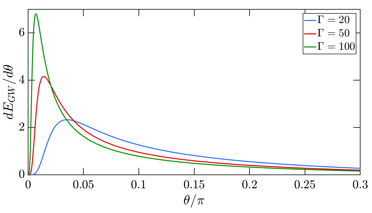
Figure 2: The angular distribution of the normalized GW energy for three different Lorentz factors. Energy is beamed in the forward direction, such that 50% of the GW energy is confined in a cone with opening angle $\sqrt{{2}/{\Gamma}}$. The area under all the distributions is normalized to unity.

Instantaneous ejection of two point particles in opposite directions will lead to a wave form that is the sum of the two

$$h(\theta_{\rm v})=\frac{4{\cal E}\beta^{2}}{r}\frac{1-\cos^{2}\theta_{\rm v}}{1-\beta^{2}\cos\theta_{\rm v}^{2}}\ .$$ (9)

$h(\theta_{\rm v})$ is almost flat apart from the minima along the two axes. However, the energy is still beamed in cones of width $\sqrt{2/\Gamma}$, as the contribution of the particle that is moving away from the observer will be seen only at much lower frequencies than the one moving towards it.

II.2 A Narrow stream - $\theta_{\rm j}=0$ and $t_{\rm inj}\neq 0$

Relaxing somewhat the ZFL approximation, we generalize the previous results to a continuous ejection of a narrow stream over $t_{\rm inj}$. All one needs to do is to integrate the single particle $h$ (Eq. 9) over the emission time. As all particles contribute with the same phase, there is no destructive interference. The final jump in the GW signal remains the same and so is the angular structure and the maximal viewing angle. There are though two important differences. The amplitude increases following $m(t)$ on a time scale $t_{\rm inj}$. (see §III below). This results in a typical frequency of $1/t_{\rm inj}$ that determines both the temporal structure of $h$ and the total energy emitted, as already discussed in Eq. 8.

II.3 A Spherical Cap - $\theta_{\rm j}\neq 0$ and $t_{\rm inj}=0$

We consider next a thin spherical cap of particles ejected simultaneously and accelerated instantaneously. The cap is defined by its opening angle $\theta_{\rm j}$, final Lorentz factor $\Gamma$, total energy ${\cal E}$, and the angle between its center and the observer $\theta_{\rm v}$. We will assume that the cap is wide, namely $\Gamma^{-1}\ll\theta_{\rm j}$. Otherwise if $\theta_{\rm j}\lesssim\Gamma^{-1}$ the signal converges to the point-particle limit.

We define the observer’s line of sight to the emitting source as the $z$ axis of our coordinate system. The coordinates $\theta$ and $\phi$ are defined in the observer’s coordinate system in the usual manner (see Fig. 1). Without loss of generality, we define the direction of the jet as $(\theta,\phi)=(\theta_{\rm v},0)$ in the observer’s frame of reference.

The axial symmetry implies a symmetry under the transformation $\phi\rightarrow-\phi$. Therefore, the metric perturbation $h_{\rm x}$ (which is now summed over the shell) vanishes identically (see Eq. 9, and Fig. 3). In the following, we simply denote $h=h_{\rm+}$, the only non-vanishing component of the metric perturbation tensor.

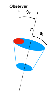
Figure 3: A schematic view of the jet (blue) for $\theta_{\rm v}<\theta_{\rm j}$. Due to the symmetry, the contribution to the GW amplitude of the part of the jet that is spherically symmetric around the observer (shown in red ) vanishes. The amplitude from partial rings with $\theta>\theta_{\rm j}-\theta_{\rm v}$, is reduced compared to the amplitude of a point-particle with the same energy and angle to the observer. The jet is symmetric under the transformation $\phi\rightarrow-\phi$: hence, the metric perturbation component $h_{\rm x}$ vanishes identically.

Integrating over the cap we find:

$$h_{\rm cap}(\theta_{\rm v},\theta_{\rm j})=\frac{2{\cal E}\beta^{2}}{r\Delta\Omega}\int_{|\theta_{\rm v}-\theta_{\rm j}|}^{min(\theta_{\rm j}+\theta_{\rm v},\pi)}\frac{\sin^{3}\theta\cdot\sin 2\Delta\phi}{1-\beta\cos\theta}d\theta\ ,$$ (10)

where $\Delta\Omega\equiv 2\pi(1-\cos\theta_{\rm j}^{2})$, the solid angle of the cap, and

$$\Delta\phi\equiv\cos^{-1}\left[\frac{\cos\theta_{\rm j}-\cos\theta_{\rm v}\cos\theta}{\sin\theta_{\rm v}\sin\theta}\right]\ .$$ (11)

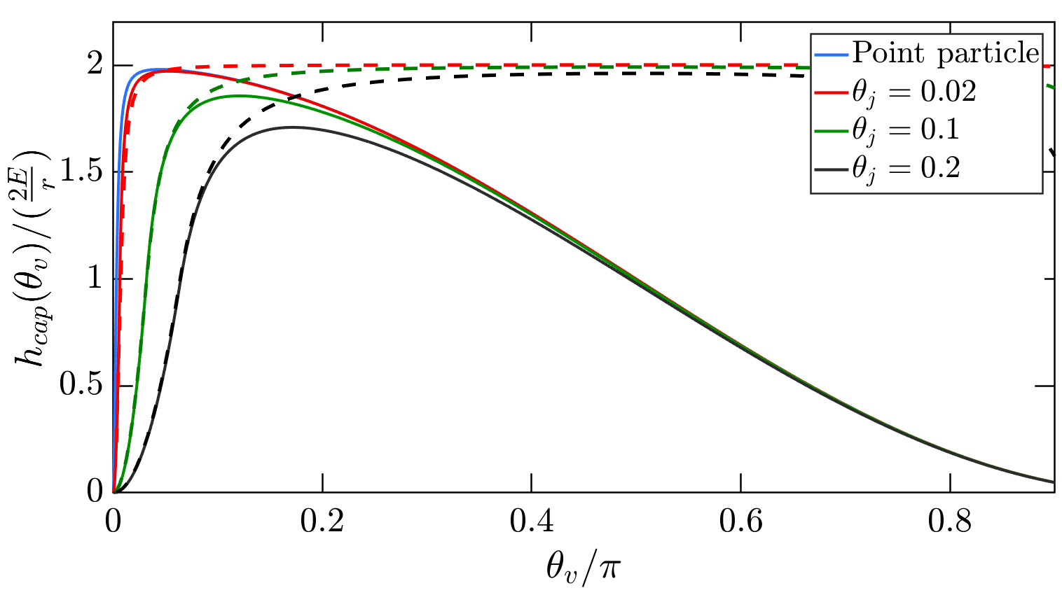
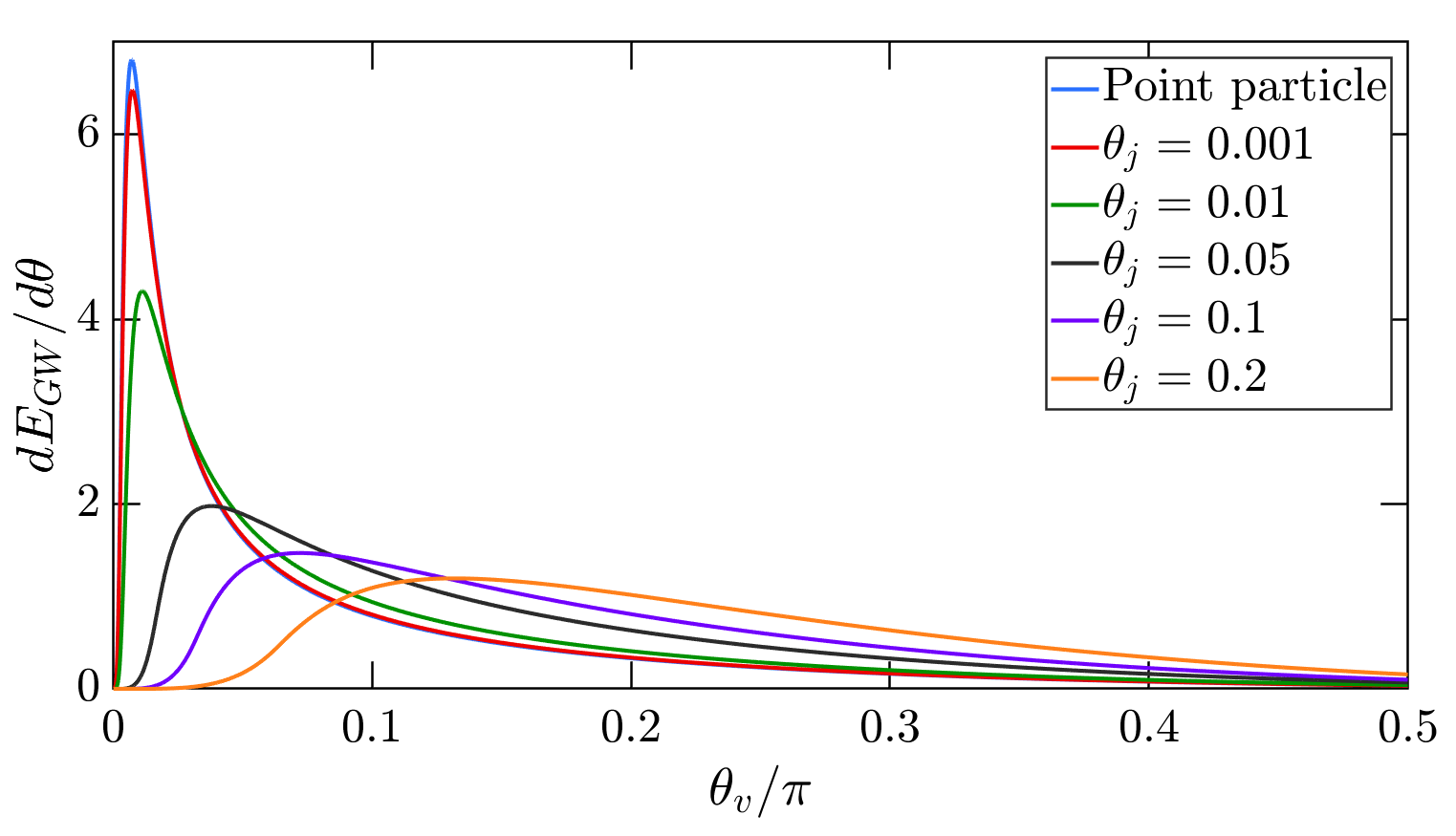
Figure 4: The angular distribution of $h$, the GW amplitude (top) and $dE_{\rm GW}/d\theta$, the normalized energy distribution (bottom) from an accelerating spherical cap with $\Gamma=100$. The anti-beaming region is $\approx 0.84\ \theta_{\rm j}$. Note the different angular scale of the two figures. The area under each energy distribution is normalized to unity. Dashed lines in the top figure represent the amplitudes of double-sided jets.

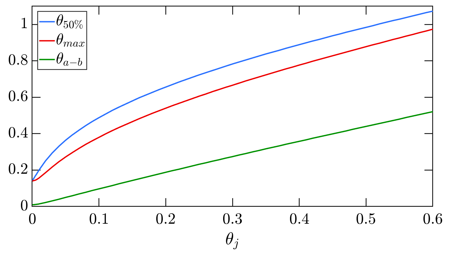
Figure 5: Specific viewing angles for a jet with $\Gamma=100$ as a function of $\theta_{\rm j}$: $\theta_{50\%}$ is the opening angle of the cone which constrains 50% of the GW’s energy, $\theta_{\rm max}$ is the viewing angle with the maximal observed GW amplitude, and $\theta_{a-b}$ is the anti-beaming angle, at which the GW amplitude drops to 50% of maximum. All plots are with $\Gamma=100$. For $\Gamma^{-1}\ll\theta_{\rm j}$, all three angles are determined by $\theta_{\rm j}$. The intercepts with the $\theta_{\rm j}=0$ axis are determined by the point-particle results.

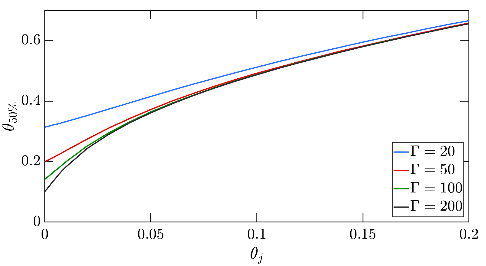
Figure 6: The GW energy beaming angle, $\theta_{50\%}$, as a function of the jet’s opening angle, for jets with different Lorentz factors. The intercepts with the $\theta_{\rm j}=0$ axis correspond to $\sqrt{{2}/{\Gamma}}$, but for $\Gamma^{-1}\ll\theta_{\rm j}$, the angle $\theta_{50\%}$ is determined by $\theta_{\rm j}$. Note that the corresponding energy distribution is peaked around $\theta_{\rm j}$ and $\pi-\theta_{\rm j}$

Figure 4 depicts $h_{\rm cap}(\theta_{\rm v},\theta_{\rm j})$ for different opening angles. This angular behavior resembles the point-particle result, with a major difference: the anti-beaming region, which was $\Gamma^{-1}$ in the point-particle case, is now $\approx 0.84\ \theta_{\rm j}$ (see Fig. 5), and it is independent of $\Gamma$. This is due to the fact that any region of the cap which is axially symmetric around the observer would have no contribution to the GW amplitude. For $\theta_{\rm v}<\theta_{\rm j}$, only the outer region of the cap, with $\theta>\theta_{\rm j}-\theta_{\rm v}$, contributes. The effect is twofold: regions of the cap with $\theta<\theta_{\rm j}-\theta_{\rm v}$ have a vanishing contribution to the amplitude, and even in the outer region, destructive interference between symmetric regions will reduce the GW amplitude.

The maximal GW amplitude is now a function of $\theta_{\rm j}$ (compare with Eq. 5). For small opening angles:

$$h_{\rm max}(\theta_{\rm j})\approx\frac{4{\cal E}}{r}(1-\frac{3}{4}\theta_{\rm j})\ .$$ (12)

Using the amplitude $h_{\rm cap}(\theta_{\rm v},\theta_{\rm j})$, we calculate the total GW energy, as a straightforward generalization of Eq. 8, but now for simplicity we estimate it only for $\tilde{t}_{\rm o}$ in which we use $\Delta\theta_{\rm v}=\theta_{\rm v}+\theta_{\rm j}$:

$$E_{\rm cap}(\theta_{\rm j})=\frac{1}{16t_{\rm acc}}\int_{0}^{\pi}\frac{h_{\rm cap}(\theta_{\rm v},\theta_{\rm j})^{2}}{1-\beta\cos(\theta_{\rm v}+\theta_{\rm j})}\sin\theta_{\rm v}d\theta_{\rm v}\ .$$ (13)

Again the energy will diverge for a strictly instantaneous acceleration. To estimate the energy in a realistic case, we have to introduce a frequency cutoff that depends on the acceleration time. But because of time of flight effects, it also depends on the relation between the viewing angle and the opening angle of the jet and the final velocity: $\tilde{t}_{\rm o}=({1-\beta\cos(\theta_{\rm v}+\theta_{\rm j})}){t_{\rm acc}}.$

Similarly to the case of the GW amplitude anti-beaming angle, we find that the angle of the cone which constrains 50% of the cap GW’s energy, $\theta_{50\%}$, is determined by $\theta_{\rm j}$ and not by $\Gamma$. Fig. 5 depicts the GW amplitude’s anti-beaming angle, as well as $\theta_{50\%}$ and the angle $\theta_{\rm max}$ where the observed GW amplitude is maximized, all as a function of the jet’s opening angle $\theta_{\rm j}$. Fig. 6 shows $\theta_{50\%}$ as a function of $\Gamma$. For $\Gamma^{-1}\ll\theta_{\rm j}$, the energy beaming angle is determined only by $\theta_{\rm j}$. Fig. 4 shows the angular distribution of the GW energy for jets with different opening angles.

II.4 Double-sided jets

The angular distribution of the GW signal changes drastically if the jet is two-sided. We turn to examine two spherical caps of equal energy that are accelerated along two opposite directions. In this case, the GW amplitude is a monotonically increasing function of $\theta_{\rm v}$, up to $\pi/2$, where it is maximal (see Fig. 4). The maximal GW amplitude is:

$$h_{\rm max}(\theta_{\rm j})=\frac{4{\cal E}}{r}\cos\theta_{\rm j},$$ (14)

where ${\cal E}$ is now the total energy of both caps. The result is similar to the case of two ejected point particles but, similarly to the single-cap case, the width of the suppressed area around the axes is now of order $0.84\theta_{\rm j}$, rather than of order $\sqrt{2/\Gamma}$.

III The Temporal Structure

We turn now to consider the effect of the more detailed temporal structure of the source and the acceleration process.

III.1 Power Spectrum and Timescales

A memory-type signal, rising to an asymptotic value $h_{0}(\theta_{\rm v})$ over a timescale $t_{\rm c}(=\max[t_{\rm acc},t_{\rm inj})])$, has a characteristic Fourier transform:

$$\tilde{h}(f,\theta_{\rm v})=\begin{cases}{h_{0}(\theta_{\rm v})}/{f},\quad f\leq f_{\rm c}\\ {h_{0}(\theta_{\rm v})f_{\rm c}}{g(f)},\ \ f\geq f_{\rm c}\end{cases}$$ (15)

where $f_{\rm c}\equiv{1}/{t_{\rm c}}$ is the crossover frequency and $g(f)$, which depends on the nature of the source, decreases faster than $1/f$. As the total GW energy must be finite, the integral $\int_{0}^{\infty}{\dot{h}}^{2}(t)dt=\int_{0}^{\infty}f^{2}{\tilde{h}}^{2}(f)df$ yields an asymptotic bound of $g\propto f^{-\alpha_{\inf}}$ with $\alpha_{\inf}>3/2$.

The Fourier transform is closely related to the spectral density, which is typically used to characterize the signal-to-noise ratio of the GW:

$$S(f)\equiv\tilde{h}(f)\cdot\sqrt{f}$$ (16)

The combination of the crossover frequency, $f_{\rm c}$, and the spectral density at this frequency, $S(f_{\rm c})$, is critical to determine the detectability of the signal. The condition

$$S_{det}(f)<S(f_{\rm c})(f_{\rm c}/f)^{1/2}$$ (17)

is a necessary but not sufficient condition for the detection of this signal. For a low-frequency detector (with a typical frequency range below $f_{\rm c}$) this condition is sufficient as it will detect such event if Eq. 17 is satisfied for some frequency in its range, $f$. This detector will observe a step function. As $S(f)$ decreases faster than $f^{-1/2}$, Eq. 17 is not a sufficient condition for detection by a high frequency detector. If it is sensitive enough, a higher frequency detector can detect the relevant and interesting temporal structure that exist beyond a simple step function.

As the signal can be characterized by the crossover frequency, the following sections are concerned with identifying this frequency in the GW’s Fourier spectrum. We discuss first the simplifying limit $t_{\rm inj}=0$, in which the jet is emitted at once. We then examine the general case, of a finite $t_{\rm inj}$.

III.2 Instantaneously spherical cap - $t_{\rm acc}=0$, $t_{\rm acc}=0$

We consider here the GW signal of a single spherical cap, of angular size $\theta_{\rm j}$, that is instantaneously injected and accelerated, but the acceleration takes place at a radius $R$ rather than at the origin. We decompose the spherical cap to concentric rings around the observer. The signal from a full ring vanishes. The signal from a partial ring at an angle $\theta$ to the observer is a Heaviside step function, whose magnitude and phase are characterized by $l(\theta)e^{2i\Delta\phi}$, where $l(\theta)$ is the fraction of the ring within the cap (see Fig. 3) and $\Delta\phi$, defined by Eq. 11, is the corresponding phase.

The arrival time of the signal from this ring is $(1-\beta\cos\theta)R/c$. Integration over these (partial) rings yields the GW signal:

$$\tilde{h}_{\rm cap}(f)=\frac{2{\cal E}\beta^{2}}{r\Delta\Omega}\int_{|\theta_{\rm v}-\theta_{\rm j}|}^{\theta_{\rm v}+\theta_{\rm j}}d\theta\frac{sin^{3}\theta}{1-\beta\cos\theta}l(\theta)e^{2i\Delta\phi}$$

$$\times\frac{i}{f}e^{if(1-\beta\cos\theta)R/c},$$ (18)

where the lower integration limit is determined by the requirement that the GW contribution of a whole ring vanishes, and $\exp[{if(1-\beta\cos\theta)R/c}]/{f}$ is the Fourier transform of the Heaviside function.

The crossover frequency for this GW signal is determined by the time delay between the earliest and latest components of the signal:

$$f_{\rm c}=\frac{1}{\cos(\theta_{\rm v}-\theta_{\rm j})-\cos(\theta_{\rm v}+\theta_{\rm j})}\frac{c}{R}\ .$$ (19)

Note that generalizing this result to a non-instanteous acceleration we can use $R=ct_{\rm acc}$.

III.3 Continuously accelerating spherical cap - $t_{\rm acc}\neq 0$.

The signal from a cap that is accelerating continuously depends on the specific acceleration model. Birnholtz & Piran [11] calculated $h(t)$ for a cap accelerating according to the basic fireball GRB model [15, 16], $\Gamma\propto R$.

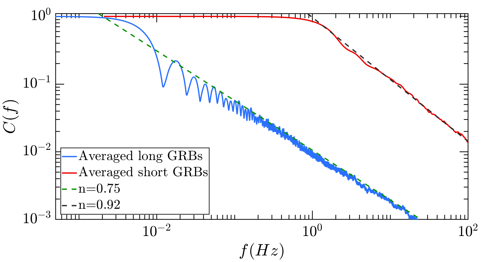
Figure 11: The averaged Fourier transform of BATSE’s long GRBs, vs. that of BATSE’s TTE short GRB catalogue. Power law fits for are shown in dashed lines.

Repeating their calculations for different $(\theta_{\rm v},\theta_{\rm j})$, we find (see Fig. 8 and also Fig. 11 of [11]) that the corresponding crossover frequency is given by the time delay between the earliest ($t=0$ at the origin) and latest ($\theta=\theta_{\rm v}+\theta_{\rm j}$ at the end of the acceleration phase) signals:

$$f_{\rm c~{}|{t_{\rm inj}=0}}=\frac{1}{1-\beta\cos(\theta_{\rm v}+\theta_{\rm j})}\frac{1}{t_{\rm acc}}$$ (20)

While this result was derived for a specific acceleration model, Eq. 20 is quite general, being derived purely from geometrical arguments. We plot in Fig. 7 the Fourier transforms of GWs based on three different acceleration models: the fireball model $\Gamma(t)-1=(\Gamma-1)t/t_{\rm acc}$; a constant acceleration in the jet’s frame of reference $\Gamma(t)^{2}-1=(\Gamma-1)^{2}(t/t_{\rm acc})^{2}$, and $\Gamma(t)-1=(\Gamma-1)\tanh(t/t^{\prime}_{\rm acc})$. For all three models, we find that the final jump in amplitude is indeed given by the ZFL limit in Eq. 10, and that the crossover frequencies are given by Eq. 20.

For all three models considered, we find that the high-frequency behavior, $g(f)$ is described by a power law $f^{-\alpha}$, with $\alpha\approx 2$. For a constant acceleration, the low-frequency behavior coincides with the fireball model. This is no surprise, since the equivalent long-timescale acceleration in both cases is $\Gamma(t)\sim t$. For the third acceleration model, the hyperbolic function’s typical timescale is not defined as clearly, so we tuned its timescale parameter, $t^{\prime}_{\rm acc}$, such that the high-frequency power law would coincide with the two other models.

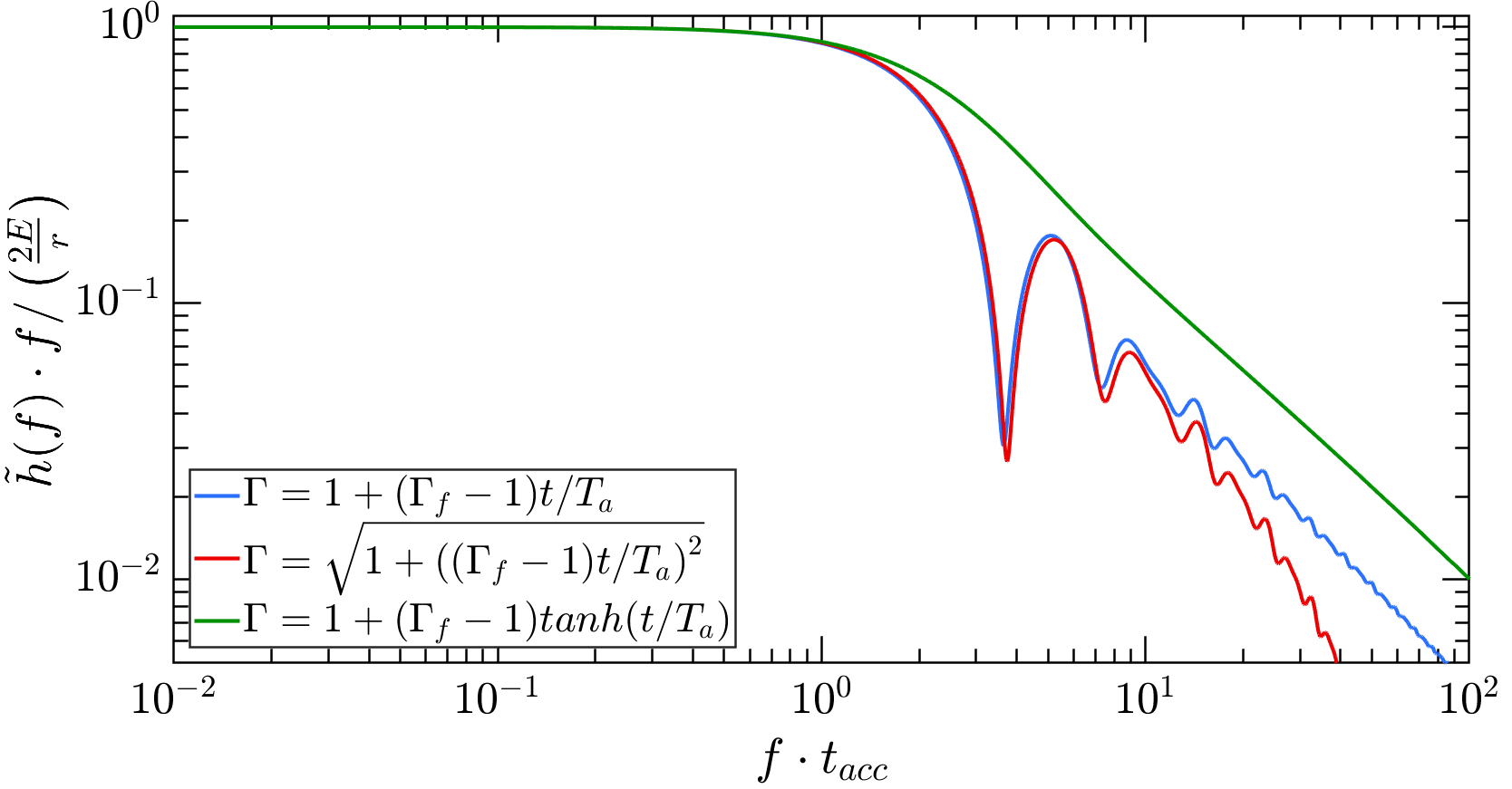
Figure 7: The Fourier transforms of $f$ from jets with three different acceleration models (with $\Gamma_{f}=100$, $\theta_{\rm j}=0.1$, $\theta_{\rm v}=0.9$). The time constant of the third model was chosen such that the high-frequency power laws would coincide.

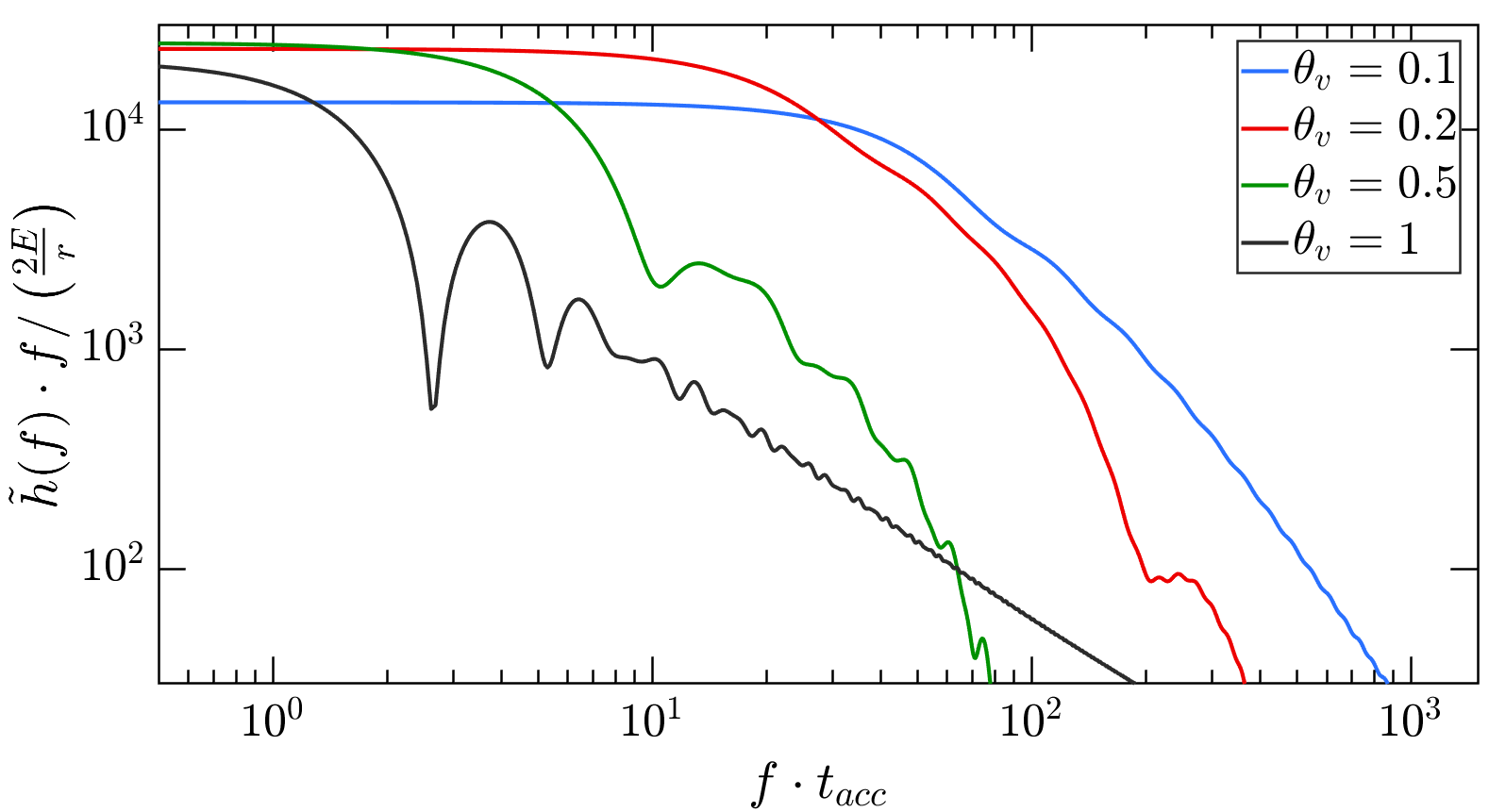
Figure 8: The normalized Fourier waveform multiplied by the frequency for jets with the acceleration model $\Gamma\propto R$, based on the numerical code describe in [11] for $\Gamma=100$ and $\theta_{\rm j}=0.1$. Below the crossover frequency, $\tilde{h}(f)\cdot f$ is a constant.

III.4 The crossover diagram

The observed frequency of the GW can get boosted by a maximal factor of $2\Gamma^{2}$ along the direction of motion of the jet. However, because of the anti-beaming, the signal is minimal in that direction. Fig. 9 depicts the crossover diagram, $S(f_{\rm c})$ vs. $f_{\rm c}$, for different jets. This diagram represents how the observed spectral density varies as it is viewed from different viewing angles.

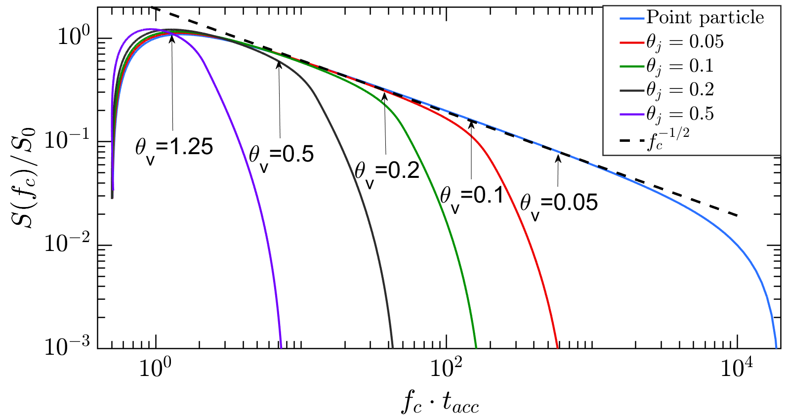
Figure 9: The crossover diagrams of jets with different opening angles, compared with that of a point particle for different opening angles (and a point particle) for $\Gamma=100$ and $t_{\rm acc}=1{\rm sec}$. The spectral density is normalized by the value $S_{0}\equiv({2{\cal E}}/{r})\sqrt{t_{\rm acc}}$. Along the curves, both the crossover frequency, $f_{\rm c}$, and the spectral density at that frequency, $S(f_{\rm c})$, vary as a function of the observer angle $\theta_{\rm v}$. Some observer angles are indicated for reference.

Figure 9 demonstrates that the jet’s finite opening angle reduces the possible boost in the crossover frequency from ${2\Gamma^{2}}$ to $({1-\cos\theta_{\rm j}})^{-1}$. While the boost in frequency increases the jet’s crossover frequency, it is always accompanied by a reduction in the observed spectral density, since the angular region in which the frequency is boosted is well within the GW’s anti-beaming region, meaning that the overall spectral density at high frequencies is diminished. The spectral density is comparable to the maximal value over a wide range of viewing angles. For example, for small opening angles ($\theta_{\rm j}<0.3$), and with $\Gamma=100$, $S(f)$ is maximal at an observer angle $\theta_{\rm v}\approx\cos^{-1}({1}/{3})=1.23$, and it exceeds 50% of the maximum value for $0.38<\theta_{\rm v}<2.17$, corresponding to 75% of the sky.

The crossover diagram of a double-headed jet, consisting of two jets propagating in two opposite directions, is rather similar to that of a single jet. This is, again, due to the anti-beaming of the GW signal. The jump in amplitude for each jet component is determined by Eq. 10. For small observer angles, the amplitude of the jet propagating away from the observer will be negligible compared to the amplitude of the jet heading towards the observer (see Fig. 4). The two jets will have comparable amplitudes only in the intermediate range of observer angles, $\theta_{\rm v}\approx{\pi}/{2}$. The contribution of both jets in this angular range is slightly higher than that of a single jet.

III.5 $t_{\rm inj}\neq 0$

With the introduction of another timescale $t_{\rm inj}$, the problem becomes more complex. The main point of the previous section, though, is unchanged: the Fourier transform of the signal is monotonically decreasing, and the crossover from $1/f$ behavior to a steeper decrease occurs at a frequency $f_{\rm c}$. The only difference between this and the $t_{\rm inj}=0$ case is the way in which the crossover frequency $f_{\rm c}$ is determined. The situation is complicated, though, because the timescale determined by the acceleration, $[1-\beta\cos(\theta_{\rm v}+\theta_{\rm j})]t_{\rm acc}$ is angle-dependent. While $t_{\rm inj}$ can be larger for some angles, the acceleration-related timescale can be larger for others.

To demonstrate the behavior we consider a toy model. In this model the signal from a single cap (i.e., a single accelerating spherical cap) is described by the function $h(t)$. The mass ejection function, $\dot{m}(t)$, describes the rate of ejection of shells. We choose a simple non-trivial model which involves two timescales:

$$h(t)=\begin{cases}0\quad&t<0\ ,\\ [{t}/{\tilde{t}_{\rm o}(\theta_{\rm v},\theta_{\rm j})}]h_{0}(\theta_{\rm v},\theta_{\rm j})\quad&0\leq t\leq\tilde{t}_{\rm o}(\theta_{\rm v},\theta_{\rm j})\ ,\\ h_{0}(\theta_{\rm v},\theta_{\rm j})\quad&t>\tilde{t}_{\rm o}(\theta_{\rm v},\theta_{\rm j})\ ;\end{cases}$$ (21)

and

$$\dot{m}(t)=\begin{cases}0\quad&t<0\ ,\\ \dot{m}_{0},\quad&0\leq t\leq t_{\rm inj}\ ,\\ 0\quad&t>t_{\rm inj}\ .\end{cases}$$ (22)

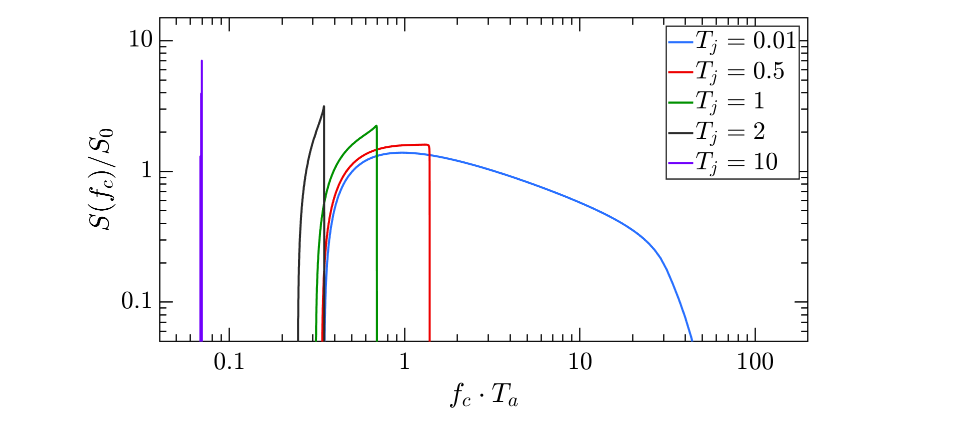
Figure 10: The crossover diagrams for jets with both $t_{\rm acc}$ and $t_{\rm inj}$. We keep $t_{\rm acc}$ fixed , with $\Gamma=100$ and $\theta_{\rm j}=0.1$ for all diagrams, and vary $t_{\rm inj}$. The amplitude $h_{0}(\theta_{\rm v},\theta_{\rm j})$ is given by Eq. 10 and the frequency $f_{\rm c}$ is then extracted from the Fourier transform of Eq. 21.

where $\tilde{t}_{\rm o}(\theta_{\rm v},\theta_{\rm j})\equiv(1-\beta\cos(\theta_{\rm v}+\theta_{\rm j}))t_{\rm acc}$ and $h_{0}(\theta_{\rm v},\theta_{\rm j})$ is the (ZFL) jump of the GW amplitude, given by Eq. 10. The combined GW signal is given by the convolution of the two functions. The amplitude of the Fourier transform at the crossover frequency is $h_{0}(\theta_{\rm v},\theta_{\rm j})/{f_{\rm c}}$. The observed crossover frequency is now determined by two timescales, and one of those, $\tilde{t}_{\rm o}(\theta_{\rm v},\theta_{\rm j})$, varies with $\theta_{\rm v}$. Fig. 10 depicts the crossover diagrams determined by the simple model of eqs. 21 - 22 .

For $t_{\rm inj}\ll\tilde{t}_{\rm o}$, we recover the previously described crossover diagram. For $t_{\rm inj}>\tilde{t}_{\rm o}$, the injection time acts as an upper cutoff on the crossover frequency. For $t_{\rm inj}\gg t_{\rm acc}$ (which implies $t_{\rm inj}\gg\tilde{t}_{\rm o}$ for all observers) the crossover diagram is reduced to a single frequency determined by $t_{\rm inj}$, independent of $\theta_{\rm v}$. Clearly, if several timescales are involved in the function $\dot{m}(t)$, it is the longest one that determines the crossover frequency. The shorter timescales will only affect the higher-frequency range of the Fourier spectrum.

IV An Example - GWs from GRB light curves

The results of the previous section were based on a simplified model for the mass flux of the jet $\dot{m}(t)$. Here, we examine a possibly more realistic description. For this we consider GW emission from GRB jets assuming that the GRB light curves follow $\dot{m}(t)$ to some extent.

Specifically, Kobayashi et al., [17] have shown that within the internal shocks model [18, 19, 20] the GRB light curve is related to $\dot{m}(t)$. This relation is not one-to-one and, moreover, current understanding suggests that the temporal structure may originate in the interaction of the jet with stellar material (in long GRBs) or with the ejecta (in short ones). Still, in the following, we use the GRB light curves as indicators for $\dot{m}(t)$, and estimate the corresponding GW signal. For a given acceleration model, the Fourier transform of the GW signal will be proportional to the convolution of the Fourier transform of the GRB light curve with the GW signal of a single shell $h_{\rm cap}(t)$. We calculate, under these assumptions, the average GW spectra for long and short GRBs observed by the Burst and Transient Source Experiment (BATSE). We use a Fourier transform, $\tilde{h}(f)$, of a single accelerating spherical cap (Eq. 15), with $\tilde{f}_{\rm o}\equiv{1}/{\tilde{t}_{\rm o}(\theta_{\rm v},\theta_{\rm j})}$ and $g(f)=f^{-\alpha}$ with $\alpha>3/2$ being the high-frequency power law from the acceleration model Fourier transform. The following calculations will proceed with a general $\alpha$, which is determined by the specific acceleration model.

IV.1 Long GRBs

Beloborodov et al. [21] calculated the average Fourier transform, $C_{\it l}(f)$, of 527 long GRB light curves observed by BATSE:

$$C_{\it l}(f)\propto\begin{cases}{\mathrm{c}onst.},\quad\quad f<f_{\it{l}}\\ f^{-0.75},\ \ \quad f>f_{\it{l}}\end{cases}\ ,$$ (23)

where the spectrum changes its slope at $f_{\it{l}}\approx 0.01Hz$. As such, the Fourier transform of the GW signal, $\tilde{h}_{\it l}(f)$, will be (see Fig. 13):

$$\tilde{h}_{\it l}(f)=C_{\it l}(f)\tilde{h}(f)\propto\begin{cases}f^{-1},\quad\quad\quad f<f_{\it{l}}\\ f^{-1.75},\quad\quad f_{\it{l}}<f<\tilde{f}_{\rm o}\\ f^{-0.75-\alpha},\quad\tilde{f}_{\rm o}<f\ .\end{cases}$$ (24)

The low-frequency behavior of the Fourier transform always behaves like $1/f$. The introduction of a new timescale means that there are two crossover frequencies, between three different power laws. In the intermediate range $f_{\it{l}}<f<\tilde{f}_{\rm o}$ the power law is determined purely by the GRB light curve, namely by the mass injection function. The unknonw high-frequency power law of the acceleration model, $\alpha$, appears only at frequencies higher than the acceleration model’s crossover frequency.

IV.2 Short GRBs

The temporal behavior of short GRBs is different from that of long ones. We repeated the above procedure, now using the TTE dataset from BATSE’s measurements, which details the arrival times of individual photons. Using a bin size of $10$msec, finding the average Fourier transform of short GRBs:

$$C_{\it s}(f)\propto\begin{cases}{\mathrm{c}onst.},\quad\quad f<f_{\it{s}}\\ f^{-0.92},\ \ \quad f>f_{\it{s}}\end{cases}$$ (25)

The high frequency power law of the short GRBs power spectrum is stiffer, and their break frequency is higher, at $f_{\it{s}}\approx 1Hz$, corresponding to the timescale of an average short GRB (see Fig. [11]). The Fourier transform of the corresponding GW signal of a short GRB takes the form:

$$\tilde{h}_{\it s}(f)=C_{\it s}(f)\tilde{h}(f)\propto\begin{cases}f^{-1},\quad\quad\quad f<f_{\it{s}}\\ f^{-1.92},\quad\quad f_{\it{s}}<f<\tilde{f}_{\rm o}\\ f^{-0.92-\alpha},\quad\tilde{f}_{\rm o}<f\end{cases}$$ (26)

This result holds only if $f_{\it{s}}<f_{obs}$. The Fourier transform of the short GRBs, $C_{\it s}$, allows for the interesting scenario in which this is not the case, and the observed acceleration timescale $\tilde{t}_{\rm o}(\theta_{\rm v},\theta_{\rm j})$ may be longer than the mass ejection timescale $t_{\rm inj}$. In this case, the form of the GW’s Fourier transform will be slightly different. At low and very high frequencies, the Fourier transform still behaves like $1/f$ and $f^{-0.92-\alpha}$, correspondingly. However, in the intermediate frequency range $\tilde{f}_{\rm o}<f<f_{\it{s}}$, the power law will be different:

$$\tilde{h}_{\it s}(f)=C_{\it s}(f)\tilde{h}(f)\propto\begin{cases}f^{-1},\quad\quad\quad f<\tilde{f}_{\rm o}\\ f^{-\alpha},\quad\quad\quad\tilde{f}_{\rm o}<f<f_{\it{s}}\\ f^{-0.92-\alpha},\quad f_{j}<f\end{cases}$$ (27)

The two cases are illustrated in Fig. 13, where we plot the Fourier transforms of two short GRB’s GWs using the Fireball acceleration model: one with $t_{\rm inj}>\tilde{t}_{\rm o}(\theta_{\rm v},\theta_{\rm j})$, and one with $t_{\rm inj}<\tilde{t}_{\rm o}(\theta_{\rm v},\theta_{\rm j})$. As it turns out, for $\alpha\approx 2$ the power laws of the intermediate frequency range in both cases are quite similar.

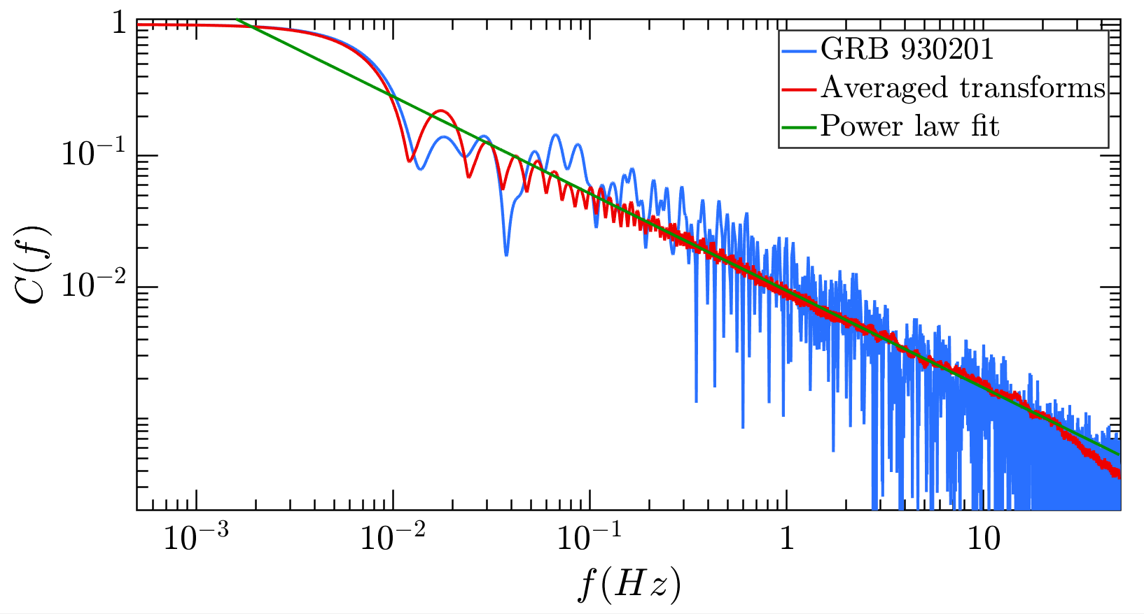
Figure 12: The Fourier transform of the light curve GRB 930201, one of the brightest bursts observed by BATSE from the BATSE data (blue). The averaged Fourier transforms of all bursts observed by BATSE (red). A power-law fit $f^{-n}$ for the average of the Fourier transforms, with $n=0.75$ (green). When averaging over many different bursts, the noise components cancel out. The frequency where the the Fourier transofrm of GRB 930201 levels out to a constant is determined by the duration of the GRB.

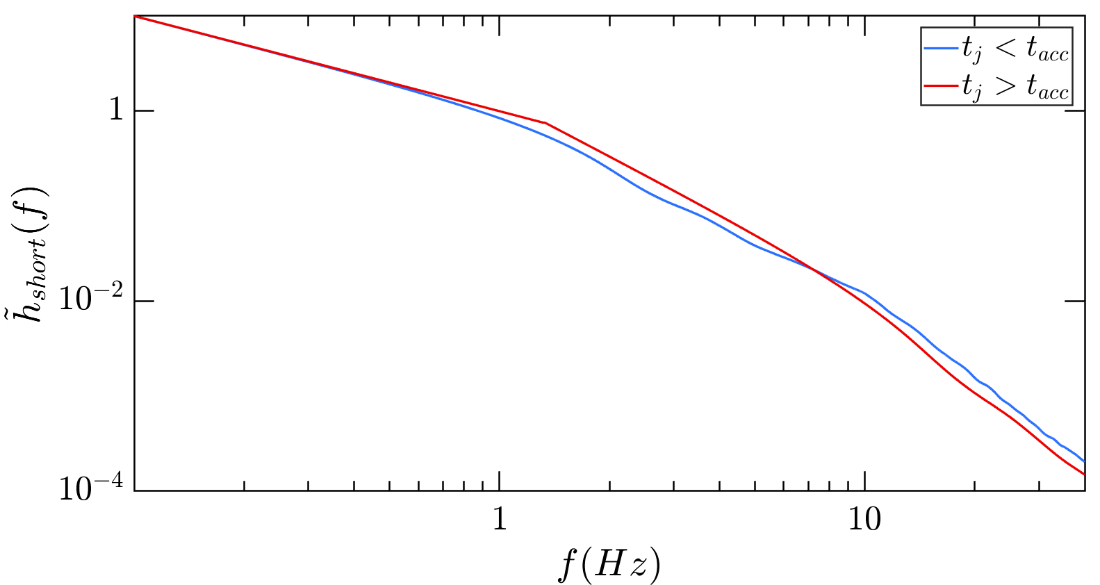
Figure 13: The Fourier transform for a short GRB’s GW calculated with $t_{\rm inj}=1{\rm sec},\tilde{t}_{\rm o}(\theta_{\rm v})=0.1{\rm sec}$ (blue), and with $t_{\rm inj}=0.1{\rm sec},\tilde{t}_{\rm o}(\theta_{\rm v})=1{\rm sec}$ (red). The power laws in the intermediate frequency region between $f_{\it{s}}$ and $\tilde{f}_{\rm o}$ are slightly different for the two cases: $\tilde{h}\propto f^{-1.92}$ for $t_{\rm inj}>\tilde{t}_{\rm o}(\theta_{\rm v})$, and $\tilde{h}\propto f^{-\alpha}$ for $t_{\rm inj}<\tilde{t}_{\rm o}(\theta_{\rm v})$.

V Detectability

When estimating the detectability of a GW signal, we have to compare the expected $S(f)$ to the detector’s sensitivity curve, $S_{\rm det}$, taking into account both the amplitude and the relevant frequency range. As we have seen in §III, for jet GW signals S(f) is always a decreasing function of the frequency. At the lowest frequency range $S(f)\propto f^{-1/2}$, while at higher frequencies (above the relevant crossover frequency) it decrease faster. Hence, a typical low-frequency detector will be most sensitive to a jet GW signal at its lowest end of its frequency response. For our purposes we can define this point as the lowest frequency below which $S_{\rm det}$ is steeper than $f^{-1/2}$. A similar condition holds for a high-frequency detector (that is, above a crossover frequency) for which we replace the power $f^{-1/2}$ by the corresponding frequency dependence of the spectral density.

Not surprisingly, like almost any relativistic GW source, the maximal amplitude of the jet GW is of order

$$h\approx\frac{G{\cal E}}{c^{4}r}=3\times 10^{-25}\bigg{(}\frac{{\cal E}}{10^{51}~{}{\rm erg}}\bigg{)}~{}\bigg{(}\frac{100{\rm Mpc}}{r}\bigg{)}\ .$$ (28)

For a one-sided jet this estimate is valid for an observer that is at optimal angle, namely at $\theta_{\rm v}\approx\theta_{\rm j}$. For two-sided jets, this estimate is valid for most observers apart from those along the jets ( $\theta_{\rm v}<\theta_{\rm j}$). Different observers will, however, observer different characteristic frequencies as discussed earlier, with the relevant frequency is the lowest crossover frequency, $f_{\rm c}$.

V.1 GW from GRB jets

GRB jets are the most natural sources for these kind of GWs. For an optimal observer near the jet, when considering the estimates based on the GRB light curves discussed in §IV, the crossover frequency is dominated by $t_{\rm inj}$ for both long and short GRBs. Thus, $f_{\rm c}=f_{\it{l}}=0.01$ Hz for the long and $f_{\rm c}=f_{\it{s}}=1$ Hz for short GRBs. This frequency range puts the events below the frequency limits of current LIGO-Virgo-Kagra, but around the capability of the planned BBO [22] and DECIGO [23]. Observers further away from the jet axis will see lower characteristic frequencies, which are even more difficult to detect.

As seen in the crossover diagram (Fig. 9), any potential increase in the frequency of the spectral density due to the boost of the crossover frequencies for observers close to the jet’s axis will be more than balanced out by the anti-beaming of the GW amplitude, such that the spectral density never benefits from observation-angle effects. Short GRBs have higher crossover frequencies and hence are somewhat easier to detect. These bursts are observed from typically nearer distances since they are intrinsically weaker and hence their observed rate is lower. However their intrinsic rate is larger by about a factor of ten than the rate of long ones. Still, due to current LIGO-Virgo-Kagra lower frequency threshold in the $10$s Hz range, which is above the expected crossover frequencies of short GRBs and definitely long GRBs, it is unlikely for any GW signal from either short or long GRB jet to be detected by these detectors. While these GRB jets GW signals are within the frequency range of BBO and DECIGO, most GRBs take place at distances that are beyond the detection horizon.

V.2 GW 170817A

At $\approx 40$ Mpc, GW170817A was an exceptionally nearby binary neutron star merger. The merger GW signal was accompanied by a short (albeit atypical – see e.g. [24, 24, 25]) GRB. The event and its afterglow signature were extremely well observed, and we have good estimates for most of its parameters. The jet properties are ${\cal E}\approx 10^{50}$erg, $\theta_{\rm v}\approx 20^{o}$, $\theta_{\rm j}\approx 5^{o}$. Other parameters, and in particular $t_{\rm acc}$ and $t_{\rm inj}$ that are most relevant for our analysis, are less known. The injection duration $t_{\rm inj}$, is capped from above by the duration of the observed $\gamma$-rays. However, as those arose from a cocoon shock breakout [24, 26] the observed duration gives only an upper limit on $t_{\rm inj}$ . In the following we assume that $t_{\rm acc}<t_{\rm inj}=1$ sec. $\Gamma$, is also unknown but it only factors into the result through ${\cal E}$, since $\Gamma^{-1}\ll\theta_{\rm j}$: hence, it is unimportant. Given the viewing angle and the jet angle, it was also ideally positioned in terms of the strength of the GW signal from its jet. That is, we were not within the anti-beamed jet’s cone but not too far from it either. Still, the jet GW that we consider here could not have been detected by current detectors. Fig. 14, depicts the spectral density of GW170817 compared with the sensitivity thresholds of GW detectors [27]. We find that the GW would have been detectable by the Big Bang Observer (BBO)[28], and would have been marginally detectable by DECIGO[29] as we discuss below..

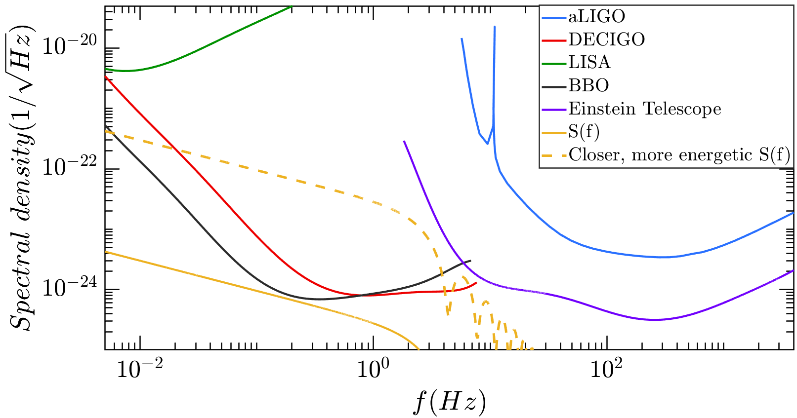
Figure 14: The calculated spectral density for our fiducial model for GW170817, $S(f)$, compared with the sensitivity thresholds of GW detectors taken from http://gwplotter.com. The dashed line shows the GW emission from the same source, only 10 times closer and 10 times more energetic. Such a signal would correspond to a CCSNe jet

We quantify detection distances by considering the signal-to-noise ratio, $\rho$, of a certain GW signal, with Fourier transform $\tilde{h}(f)$ [27]:

$$\rho^{2}=4\int_{-\infty}^{\infty}\frac{\tilde{h}(f)^{2}}{S_{n}(f)^{2}}df,$$ (29)

where $S_{n}(f)$ is the detector’s noise amplitude.

We find that the most suitable detector for observing jet GWs is BBO, with a detection horizon of $r_{d}=75$Mpc. DECIGO closely follows, with $r_{d}=40$Mpc. The Einstein telescope has $r_{d}=600$kpc, and LISA is at $r_{d}=80$ kpc. Ultimate DECIGO which will be about hunderd time more sensitve than DECIGO will detect such events from distances of a few Gpc, that is up to $z=0.5$. These distances scale linearly with the jet’s energy: a jet with a short duration like GW170817 but with $E=10^{51}$ erg will be detectable by DECIGO up to a distance of $400$ Mpc, etc.

A higher GW crossover frequency, $f_{\rm c}$, increases the maximal detection distance $r_{d}$. Notably, however, $r_{d}$ approaches an asymptotic value, and increasing $f_{\rm c}$ above a certain detector-specific threshold does not change that detector’s maximal detection distance. This is because the integral in Eq. 29 is dominated by the part of the GW’s Fourier transform which is within the detector’s frequency band. If $f_{\rm c}$ is higher than this band, then the integral is dominated by the low-frequency $\sim 1/f$ behavior of the transform, which is independent of $f_{\rm c}$. When $f_{\rm c}$ is within the detector’s frequency band, the SNR will be reduced, due to the integration over the higher-frequency region of the GW, which behaves as $\sim 1/f^{2}$.

V.3 Jets in Core Collapse SNe and low-luminosity GRBs

The prospects for CCSNe-related GW detection are much more optimistic. Shortly after the discovery of the first low-luminosity GRB 980415 (that was associated with SN98bw) it was suggested [3, 4, 5] that the emission arose from shock breakout following an energetic jet that was choked deep in the accompanying star. Later on it was realized that, while the detection rate of low-luminosity GRBs is much lower than that of regular long GRBs, their actual rate is orders of magnitude larger [6, 7]. The detection rate is small because, given their low luminosity, they are detected only from relatively short distances. More recently, Piran et al. [30] have shown that a significant fraction of CCSNe (that are not associated with GRBs) contain an energetic ($\sim 10^{51}$ erg) choked relativistic jet. While this jet is relativistic, it is chocked inside the star depositing its energy into a cocoon. Upon breakout the cocoon material is observed as a high velocity (0.1-0.2c) material that engulfs the supernova and can be detected within the first few days. Such signatures have been detected as early as 1997 [31] in SN 1997EF and in several other SNe since then. This suggestion was nicely confirmed with the exquisite observations of this high velocity material in SN 2017iuk by [8, 9]. If such relativistic jets are associated with a significant fraction of CCSNe then, as the supernova rate is significantly larger than GRB rate [16], we can expect much nearer jets that would be sources of such GWs.

Comparing relativistic SNe Jets with GRB jets, we estimate $h$ to be a factor of 100-1000 larger than the one estimated for short GRBs: a factor of 10 in the distance (tens of Mpc vs. hundreds of Mpc) and a factor of 10-10 in energy ($10^{51}$ erg vs. $10^{49-50}$ erg). Thus, we expect amplitudes of $3\times 10^{-24}$ (see Eq. 28). Unfortunately, for these events we don’t have a good clue on $t_{\rm inj}$. A best guess is that it will be of the same order as the one estimated in long GRB, namely of order of a few tens of seconds. Thus, the corresponding crossover frequency would be around 0.01 Hz. However, on average we will observe these events from a large viewing angle, and in this case the crossover frequency would be even lower. The exact value will depend on $t_{\rm acc}$, and in turn on the unknown nature of the acceleration process.

V.4 Contribution to the GW background

The relativistic jets that arise from GRBs (both long and short) and hidden jets in SNe produce a continuous background of jet-GW waves at frequency range of $\sim 0.01-1$Hz depending on the specific source. Both long and short GRBs are rare and won’t make a significant contribution to such a background. However, SNe take place at a rate of about one per second in the observable Universe. If a significant fraction of SNe harbor energetic jets the time between two such cosmological events, a few seconds, will be comparable to the characteristic time scale of the GW signals from these jets (assuming that the hidden jets in SNe are similar in nature to GRB jets). Depending on the ratio of the time between events and the characteristic frequency of the jet-GW signal we expect either a continuous background, as expected from the GW background from merging binary neutron stars, or a pop-corn like signature, as expected for the GW background from merging binary black holes [32]. With a typical cosmological distance of a few Gpc the corresponding amplitude of this jet-GW background is $h\approx 10^{-26}{\cal E}/(10^{51}{\rm erg})$.

VI Discussion

We have obtained the qualitative and quantitative behavior of the amplitude, the angular distribution of both $h$ and $dE_{\rm GW}/d\Omega$, and the Fourier transform of the GW signal of an accelerated jet with an opening angle $\theta_{\rm j}$. The signal is anti-beamed away from the direction of the jet. The anti-beaming angle is $\max(\Gamma^{-1},\theta_{\rm j}$). Like typical relativistic GW sources, the amplitude is of order $G{\cal E}/c^{4}r$. However, unlike other sources, the signal here is of a memory type, rising to this amplitude on a characteristic time scale. The signal can be approximated as a step function when considering detectors whose typical response frequency is much lower than the characteristic crossover frequency of the jet. This last feature is of course problematic, as it might be difficult to distinguish this signal from other step functions that may arise in GW detectors. We won’t explore the experimental/observational aspects of this question.

The light curve depends on two timescales: the acceleration timescale $t_{\rm acc}$, and the mass ejection time $t_{\rm inj}$. The spectral density $S(f)$ is monotonically decreasing with the frequency. It is broken into at least two power laws: the lower frequency region is proportional to $f^{-1/2}$, and the higher frequency region is proportional to $f^{-1/2-\alpha}$, with $\alpha>3/2$. The spectral density is characterized by the crossover region, $f_{\rm c}$, which corresponds to the longest relevant timescale. Since $S(f)$ decreases monotonically with frequency, the crossover region is a good indicator as to whether a given GW’s signal can be measured by a specific detector.

The universal form of the ’crossover diagrams’ describe how the frequency and the amplitude of the spectral density shift due to the dependence of the observed amplitude and frequency on $\theta_{\rm v}$. We calculated these ’crossover diagrams’ for a point particle, a jet with a finite opening angle, a double-headed jet, as well as for jets with both $t_{\rm acc}$ and $t_{\rm inj}$. For $t_{\rm inj}\gg t_{\rm acc}$, the crossover diagram is reduced to a single characteristic frequency for observers at all angles.

Assuming that the observed GRB light curves are proportional to the jet’s mass ejection function $\dot{m}(t)$ and assuming a specific acceleration model, we calculated possible examples of expected GW signals from long and short GRBs jets. As expected, we find that the composite Fourier transforms are monotonically decreasing, and that they are described by two crossover frequencies, between three power laws. One crossover frequency is associated with $t_{\rm inj}$, and the other is associated with $t_{\rm acc}$. It is important to note, however, that these estimates should be considered just as examples.

Recent understanding of jet propagation in dense media suggests that the injection must be longer than the observed duration of the GRB [7]. Thus, the latter puts a lower limit on $t_{\rm inj}$. However, the light curves of short GRBs suggest that in many cases mergers produce jet that are choked inside the merger ejecta. Those events are not accompanied by a short GRB [33]. In such a case, $t_{\rm inj}$ can be much shorter (this is the reason that the jet was choked), and the corresponding GW signal will have a higher frequency.

As an example, we calculated the gravitational waveform of the GW emitted by the jet associated with GW170817 under the previous assumptions. Using the event’s parameters, we found that the jet’s GW could have been observed by BBO and DECIGO. Within the limiting assumptions that the duration of the burst and the observed $\gamma$-ray light curve reflect the injection time, the relevant frequencies are quite low, and indeed BBO and DEGIGO are the most suitable detectors for observing GWs from similar short GRB jets. Anti-beaming will, however, make it unlikely that we would observe both the $\gamma$-rays and the GWs. However, other multimessenger signals, and in particular GWs from the merger itself, would accompany such an event triggering our attention and providing a additional significance to the detected GW signal. It is interesting to remark that the jet launching can be delayed by as much as a second after the merger, and, as such, this GW signal can be easily separated from the more “regular” pre-merger GW emission, and even from the post-merger ringdown of the proto-neutron star and collapse to a black hole.

While the detection prospects of a jet GW signature from short or long GRBs are not that promising, comparable or even more powerful relativistic jets also take place within some core collapse SNe. The rate of these events is much larger, and correspondingly within a given observing time frame they will take place at much nearer distances. Here the detection prospects are very promising once detectors in the sub-Hz are available. A detection would reveal features of jet acceleration in the vicinity of black holes that are impossible to find in any other way.