A Product Space Reformulation with Reduced Dimension for Splitting Algorithms

Abstract

In this paper we propose a product space reformulation to transform monotone inclusions described by finitely many operators on a Hilbert space into equivalent two-operator problems. Our approach relies on Pierra’s classical reformulation with a different decomposition, which results on a reduction of the dimension of the outcoming product Hilbert space. We discuss the case of not necessarily convex feasibility and best approximation problems. By applying existing splitting methods to the proposed reformulation we obtain new parallel variants of them with a reduction in the number of variables. The convergence of the new algorithms is straightforwardly derived with no further assumptions. The computational advantage is illustrated through some numerical experiments.

Keywords

Pierra’s product space reformulation $\cdot$ Splitting algorithm $\cdot$ Douglas–Rachford algorithm $\cdot$ Monotone inclusions $\cdot$ Feasibility problem $\cdot$ Projection methods

MSC 2020:

47H05 $\cdot$ 47J25 $\cdot$ 49M27 $\cdot$ 65K10 $\cdot$ 90C30

1 Introduction

A problem of great interest in optimization and variational analysis is the monotone inclusion consisting in finding a zero of a monotone operator. In many practical applications, such operator can be decomposed as a sum of finitely many maximally monotone operators. The problem takes then the form

$$\text{Find }x\in\mathcal{H}\text{ such that }0\in A_{1}(x)+A_{2}(x)+\cdots+A_{r}(x),$$ (1.1)

where $\mathcal{H}$ is a Hilbert space and $A_{1},A_{2},\ldots,A_{r}:\mathcal{H}\rightrightarrows\mathcal{H}$ are maximally monotone. When the sum is itself maximally monotone, in theory, inclusion (1.1) could be numerically solved by the well-known proximal point algorithm [42]. However, this method requires the computation of the resolvent of the whole operator at each iteration, which is not usually available. In fact, computing the resolvent of a sum at a given point $q\in\mathcal{H}$, i.e.,

$$\text{Find }p\in J_{\sum_{i=1}^{r}A_{i}}(q),$$ (1.2)

where $J_{A}$ denotes the resolvent of an operator $A$, is a problem of interest itself which arises in some optimization subroutines as well as in direct applications such as best approximation, image denoising and partial differential equations (see, e.g., [12]).

Splitting algorithms take advantage of the decomposition and activate each operator separately, either by direct evaluation (forward steps) or via its resolvent (backward steps), to construct a sequence that converges to a solution of the problem. Splitting algorithms include, in particular, the so-called projection methods, which permit to find a point (or the closest point) in the intersection of a collection of sets by computing individual projections onto them. Classical splitting algorithms for monotone inclusions include the Forward-Backward algorithm and its variants, see, e.g., [14, 19, 34, 44], and the Douglas–Rachford algorithm [26, 33], among others (see, e.g., [14, Chapter 23]). On the other hand, different splitting algorithms for computing the resolvent of a sum can be found in, e.g, [2, 8, 20, 23]. See also the recent unifying framework [12].

Most splitting algorithms in the literature are devised for a sum of two operators, whereas there exist just a few three-operator extensions, see, e.g., [24, 41, 43]. In general, problems (1.1)–(1.2) are tackled by splitting algorithms after applying Pierra’s product space reformulation [38, 39]. This technique constructs an equivalent two-operator problem, embedded in a product Hilbert space, that preserves computational tractability in the sense that the resolvents of the new operators can be readily computed. However, since each operator in the original problem requires one dimension in the product space, this technique may result numerically inefficient when the number of operators is too large.

In this work we propose an alternative reformulation, based on Pierra’s classical one, which reduces the dimension of the resulting product Hilbert space. Our approach consists in merging one of the operators with the normal cone to the diagonal set, what allows to remove one dimension in the product space. In fact, this seems a more natural embedding than Pierra’s one since it reproduces exactly the original problem when this is initially defined by two operators (see Remark 3.4). We would like to note that this reformulation has already been used in other frameworks. For instance, it was employed in [31] for deriving necessary conditions for extreme points of a collection of closed sets. Our main contribution is showing that the computability of the resolvents of the new defined operators is kept with no further assumptions. This result allows us to implement known splitting algorithms under this reformulation, what traduces in the elimination of one variable defining the iterative scheme in comparison to Pierra’s approach.

After the publication of the first preprint version of this manuscript we were noticed about [21], where the authors suggest an analogous dimension reduction technique for structured optimization problems. Although that reformulation is different, the derived parallel Douglas–Rachford (DR) algorithm seems to lead to a scheme equivalent to the one obtained from Theorem 5.1 in this context. Notwithstanding, our analysis is developed in the more general framework of monotone inclusions. Furthermore, we provide detailed proofs of the equivalency and resolvents formulas, as well as numerical comparison to the classical Pierra’s reformulation. On the other hand, Malitsky and Tam independently proposed in [35] another $r$-operator DR-type algorithm embedded in a reduced-dimensional space. This algorithm, which can be seen as an attempt to extend Ryu’s splitting algorithm [43] (see Remark 5.2), differs from the one proposed in this work and it will also be tested in our experiments.

It is worth mentioning that a similar idea for feasibility problems was previously developed in [22]. In there, the dimensionality reduction was obtained by replacing a pair of constraint sets in the original problem by their intersection before applying Pierra’s reformulation. However, the convergence of some projection algorithms may require a particular intersection structure of these sets. Our approach has the advantage of being directly applicable to any splitting algorithm with no additional requirements.

The remainder of the paper is organized as follows. In Section 2 we recall some preliminary notions and auxiliary results. Then Section 3 is divided into Section 3.1, where we first recall Pierra’s standard product space reformulation, and Section 3.2, in which we propose an alternative reformulation with reduced dimension. We discuss and illustrate the particular case of feasibility and best approximation problems in Section 4. In Section 5, we apply our reformulation to construct new parallel variants of some splitting algorithms. Finally, in Section 6 we perform some numerical experiments that exhibit the advantage of the proposed reformulation.

2 Preliminaries

Throughout this paper, $\mathcal{H}$ is a Hilbert space endowed with inner product $\langle\cdot,\cdot\rangle$ and induced norm $\|\cdot\|$. We abbreviate norm convergence of sequences in $\mathcal{H}$ with $\to$ and we use $\rightharpoonup$ for weak convergence.

2.1 Operators

Given a nonempty set $D\subseteq\mathcal{H}$, we denote by $A:D\rightrightarrows\mathcal{H}$ a set-valued operator that maps any point $x\in D$ to a set $A(x)\subseteq\mathcal{H}$. In the case where $A$ is single-valued we write $A:D\to\mathcal{H}$. The graph, the domain, the range and the set of zeros of A, are denoted, respectively, by $\operatorname{gra}A$, $\operatorname{dom}A$, $\operatorname{ran}A$ and $\operatorname{zer}A$; i.e.,

$$\operatorname{gra}A:=\left\{(x,u)\in\mathbb{R}^{n}\times\mathbb{R}^{n}:u\in A(x)\right\},\quad\operatorname{dom}A:=\left\{x\in\mathbb{R}^{n}:A(x)\neq\emptyset\right\},$$

$$\operatorname{ran}A:=\left\{x\in\mathbb{R}^{n}:x\in A(z)\text{ for some }z\in\mathbb{R}^{n}\right\}\quad\text{and}\quad\operatorname{zer}A:=\left\{x\in\mathbb{R}^{n}:0\in A(x)\right\}.$$

The inverse of $A$, denoted by $A^{-1}$, is the operator defined via its graph by $\operatorname{gra}A^{-1}:=\{(u,x)\in\mathbb{R}^{n}\times\mathbb{R}^{n}:u\in A(x)\}$. We denote the identity mapping by $\operatorname{Id}$.

Definition 2.1 (Monotonicity).

An operator $A:\mathcal{H}\rightrightarrows\mathcal{H}$ is said to be

1. monotone if

   $$\langle x-y,u-v\rangle\geq 0,\quad\forall(x,u),(y,v)\in\operatorname{gra}A;$$

   Furthermore, $A$ is said to be maximally monotone if it is monotone and there exists no monotone operator $B:\mathcal{H}\rightrightarrows\mathcal{H}$ such that $\operatorname{gra}B$ properly contains $\operatorname{gra}A$.

2. uniformly monotone with modulus $\phi:\mathbb{R}_{+}\to[0,+\infty]$ if $\phi$ is increasing, vanishes only at 0, and

   $$\langle x-y,u-v\rangle\geq\phi\left(\|x-y\|\right),\quad\forall(x,u),(y,v)\in\operatorname{gra}A.$$

3. $\mu$-strongly monotone for $\mu>0$, if $A-\mu\operatorname{Id}$ is monotone; i.e.,

   $$\langle x-y,u-v\rangle\geq\mu\|x-y\|^{2},\quad\forall(x,u),(y,v)\in\operatorname{gra}A.$$

Clearly, strong monotonicity implies uniform monotonicity, which itself implies monotonicity. The reverse implications are not true.

Remark 2.2.

The notions in Definition 2.1 can be localized to a subset of the the domain. For instance, $A:\mathcal{H}\rightrightarrows\mathcal{H}$ is $\mu$-strongly monotone on $C\subseteq\operatorname{dom}A$ if

$$\langle x-y,u-v\rangle\geq\mu\|x-y\|^{2},\quad\forall x,y\in C,\forall u\in A(x),\forall v\in A(y).$$

Lemma 2.3.

Let $A,B:\mathcal{H}\rightrightarrows\mathcal{H}$ be monotone operators. The following hold.

1. If $A$ is uniformly monotone on $\operatorname{dom}(A+B)$, then $A+B$ is uniformly monotone with the same modulus than $A$.

2. If $A$ is $\mu$-strongly monotone on $\operatorname{dom}(A+B)$, then $A+B$ is $\mu$-strongly monotone.

Proof.

Let $(x,u),(y,v)\in\operatorname{gra}(A+B)$, i.e., $u=u_{1}+u_{2}$ and $v=v_{1}+v_{1}$ with $(x,u_{1}),(y,v_{1})\in\operatorname{gra}A$ and $(x,u_{2}),(y,v_{2})\in\operatorname{gra}B$. (i): Suppose that $A$ is uniformly monotone on $\operatorname{dom}(A+B)$ with modulus $\phi$. Since $x,y\in\operatorname{dom}(A+B)$, we get that

$$\langle x-y,u-v\rangle=\langle x-y,u_{1}-v_{1}\rangle+\langle x-y,u_{2}-v_{2}\rangle\geq\phi(\|x-y\|),$$

which proves that $A+B$ is uniformly monotone with the same modulus. The proof of (ii) is analogous and, thus, omitted. ∎

Definition 2.4 (Resolvent).

The resolvent of an operator $A:\mathcal{H}\rightrightarrows\mathcal{H}$ with parameter $\gamma>0$ is the operator $J_{\gamma A}:\mathcal{H}\rightrightarrows\mathcal{H}$ defined by

$$J_{\gamma A}:=(\operatorname{Id}+\gamma A)^{-1}.$$

The resolvent of the sum of two monotone operators has no closed expression in terms of the individual resolvents except for some particular situations. The following fact, which is fundamental in our results, contains one of those special cases.

Fact 2.5.

Let $A,B:\mathcal{H}\rightrightarrows\mathcal{H}$ be maximally monotone operators such that $B(y)\subseteq B(J_{A}(y))$, for all $y\in\operatorname{dom}B.$ Then, $A+B$ is maximally monotone and

$$J_{A+B}(x)=J_{A}(J_{B}(x)),\quad\forall x\in\mathcal{H}.$$

Proof.

See, e.g., [14, Proposition 23.32(i)]. ∎

2.2 Functions

Let $f:\mathcal{H}\to{]-\infty,+\infty]}$ be a proper, lower semicontiuous and convex function. The subdifferential of $f$ is the operator $\partial f:\mathcal{H}\rightrightarrows\mathcal{H}$ defined by

$$\partial f(x):=\left\{u\in\mathcal{H}:\langle y-x,u\rangle+f(x)\leq f(y),\quad\forall y\in\mathcal{H}\right\}.$$

The proximity operator of $f$ (with parameter $\gamma$), $\operatorname{prox}_{\gamma f}:\mathcal{H}\rightrightarrows\mathcal{H}$, is defined at $x\in\mathcal{H}$ by

$$\operatorname{prox}_{\gamma f}(x):=\operatorname*{argmin}_{u\in\mathcal{H}}\left(f(u)+\frac{1}{2\gamma}\|x-u\|^{2}\right).$$

Fact 2.6.

Let $f:\mathcal{H}\to{]-\infty,+\infty]}$ be proper, lower semicontiuous and convex. Then, the subdifferential of $f$, $\partial f$, is a maximally monotone operator whose resolvent becomes the proximity operator of $f$, i.e.,

$$J_{\gamma\partial f}(x)=\operatorname{prox}_{\gamma f}(x),\quad\forall x\in\mathcal{H}.$$

Proof.

See, e.g., [14, Theorem 20.25 and Example 23.3]. ∎

2.3 Sets

Given a nonempty set $C\subseteq\mathcal{H}$, we denote by $d_{C}$ the distance function to $C$; that is, $d_{C}(x):=\inf_{c\in C}\|c-x\|$, for all $x\in\mathcal{H}$. The projection mapping (or projector) onto $C$ is the possibly set-valued operator $P_{C}:\mathcal{H}\rightrightarrows C$ defined at each $x\in\mathcal{H}$ by

$$P_{C}(x):=\left\{p\in C:\|x-p\|=d_{C}(x)\right\}.$$

Any point $p\in P_{C}(x)$ is said to be a best approximation to $x$ from $C$ (or a projection of $x$ onto $C$). If a best approximation in $C$ exists for every point in $\mathcal{H}$, then $C$ is said to be proximinal. If every point $x\in\mathcal{H}$ has exactly one best approximation from $C$, then $C$ is said to be Chebyshev. Every nonempty, closed and convex set is Chebyshev (see, e.g., [14, Theorem 3.16]).

The next results characterizes the projection onto a closed affine subspace.

Fact 2.7.

Let $D\subseteq\mathcal{H}$ be a closed affine subspace and let $x\in\mathcal{H}$. Then

$$p=P_{D}(x)\quad\iff\quad p\in D\,\,\text{ and }\,\,\langle x-p,d-p\rangle=0,\,\,\forall d\in D.$$

Proof.

See, e.g., [14, Corollary 3.22]. ∎

The indicator function of a set $C\subseteq\mathcal{H}$, $\iota_{C}:\mathcal{H}\to{]-\infty,+\infty]}$, is defined as

$$\iota_{C}(x):=\left\{\begin{array}[]{cl}0,&\text{if }x\in C,\\ +\infty,&\text{if }x\not\in C.\end{array}\right.$$

If $C$ is closed and convex, $\iota_{C}$ is convex and its differential turns to the normal cone to $C$, which is the operator $N_{C}:\mathcal{H}\rightrightarrows\mathcal{H}$ defined by

$$N_{C}(x):=\left\{\begin{array}[]{ll}\{u\in\mathcal{H}:\langle u,c-x\rangle\leq 0,\,\forall c\in C\},&\text{if }x\in C,\\ \emptyset,&\text{otherwise.}\end{array}\right.$$

Fact 2.8.

Let $C\subseteq\mathcal{H}$ be nonempty, closed and convex. Then, the normal cone to $C$, $N_{C}$, is a maximally monotone operator whose resolvent becomes the projector onto $C$, i.e.,

$$J_{\gamma N_{C}}(x)=P_{C}(x),\quad\forall x\in\mathcal{H}.$$

Proof.

See, e.g., [14, Examples 20.26 and 23.4]. ∎

We conclude this section with the following result that characterizes the projector onto the intersection of a proximinal set (not necessarily convex) and a closed affine subspace under particular assumptions. It is a refinement of [22, Theorem 3.1(c)], whose proof needs to be barely modified.

Lemma 2.9.

Let $C\subseteq\mathcal{H}$ be nonempty and proximinal and let $D\subseteq\mathcal{H}$ be a closed affine subspace. If $P_{C}(d)\cap D\neq\emptyset$ for all $d\in D$, then

$$P_{C\cap D}(x)=P_{C}(P_{D}(x))\cap D,\quad\forall x\in\mathcal{H}.$$

Proof.

Fix $x\in\mathcal{H}$. By assumption we have that $P_{C}(P_{D}(x))\cap D\neq\emptyset$. Pick any $c\in P_{C}(P_{D}(x))\cap D$ and let $p\in P_{C\cap D}(x)$. Then $c\in P_{C}(d)\cap D$, where $d=P_{D}(x)$. Since $D$ is an affine subspace and $d=P_{D}(x)$, we derive from Fact 2.7 applied to $c\in D$ and $p\in D$, respectively, that $\langle x-d,c-d\rangle=0$ and $\langle x-d,p-d\rangle=0$. Therefore,

$$\|x-c\|^{2}=\|x-d\|^{2}+\|c-d\|^{2}\quad\text{and}\quad\|x-p\|^{2}=\|x-d\|^{2}+\|p-d\|^{2}.$$ (2.1)

Since $c\in P_{C}(d)$ and $p\in C$ then $\|c-d\|\leq\|p-d\|$. This combined with (2.1) yields $\|x-c\|\leq\|x-p\|$. Note that $p\in P_{C\cap D}(x)$ and $c\in C\cap D$, so it must be

$$\|x-c\|=\|x-p\|.$$ (2.2)

It directly follows from (2.2) that $c\in P_{C\cap D}(x)$. Furthermore, by combining (2.2) with (2.1) we arrive at $\|c-d\|=\|p-d\|$, which implies that $p\in P_{C}(d)\cap D$ and concludes the proof. ∎

3 Product space reformulation for monotone inclusions

In this section we introduce our proposed reformulation to convert problems (1.1)–(1.2) into equivalent problems with only two operators. To this aim, we first recall the standard product space reformulation due to Pierra [38, 39].

3.1 Standard product space reformulation

Consider the product Hilbert space $\mathcal{H}^{r}=\mathcal{H}\times\stackrel{{\scriptstyle(r)}}{{\cdots}}\times\mathcal{H}$, endowed with the inner product

$$\langle\boldsymbol{x},\boldsymbol{y}\rangle:=\sum_{i=1}^{r}\langle x_{i},y_{i}\rangle,\quad\forall\boldsymbol{x}=(x_{1},x_{2},\ldots,x_{r}),\boldsymbol{y}=(y_{1},y_{2},\ldots,y_{r})\in\mathcal{H}^{r},$$

and define

$$\boldsymbol{D}_{r}:=\left\{(x,x,\ldots,x)\in\mathcal{H}^{r}:x\in\mathcal{H}\right\},$$

which is a closed subspace of $\mathcal{H}^{r}$ commonly known as the diagonal. We denote by $\boldsymbol{j}_{r}:\mathcal{H}\to\boldsymbol{D}_{r}$ the canonical embedding that maps any $x\in\mathcal{H}$ to $\boldsymbol{j}_{r}(x)=(x,x,\ldots,x)\in\boldsymbol{D}_{r}$. The following result collects the fundamentals of Pierra’s standard product space reformulation.

Fact 3.1 (Standard product space reformulation).

Let $A_{1},A_{2},\ldots,A_{r}:\mathcal{H}\rightrightarrows\mathcal{H}$ be maximally monotone and let $\gamma>0$. Define the operator $\boldsymbol{A}:\mathcal{H}^{r}\rightrightarrows\mathcal{H}^{r}$ as

$$\boldsymbol{A}(\boldsymbol{x}):=A_{1}(x_{1})\times A_{2}(x_{2})\times\cdots\times A_{r}(x_{r}),\quad\forall\boldsymbol{x}=(x_{1},x_{2},\ldots,x_{r})\in\mathcal{H}^{r}.$$ (3.1)

Then the following hold.

1. $\boldsymbol{A}$ is maximally monotone and

   $$J_{\gamma\boldsymbol{A}}(\boldsymbol{x})=\left(J_{\gamma A_{1}}(x_{1}),J_{\gamma A_{2}}(x_{2}),\cdots,J_{\gamma A_{r}}(x_{r})\right),\quad\forall\boldsymbol{x}=(x_{1},x_{2},\ldots,x_{r})\in\mathcal{H}^{r}.$$

2. The normal cone to $\boldsymbol{D}_{r}$ is given by

   $$N_{\boldsymbol{D}_{r}}(\boldsymbol{x})=\left\{\begin{array}[]{ll}\boldsymbol{D}_{r}^{\perp}=\{\boldsymbol{u}=(u_{1},u_{2},\ldots,u_{r})\in\mathcal{H}^{r}:\sum_{i=1}^{r}u_{i}=0\},&\text{if }\boldsymbol{x}\in\boldsymbol{D}_{r},\\ \emptyset,&\text{otherwise.}\end{array}\right.$$

   It is a maximally monotone operator and

   $$J_{\gamma N_{\boldsymbol{D}_{r}}}(\boldsymbol{x})=P_{\boldsymbol{D}_{r}}(\boldsymbol{x})=\boldsymbol{j}_{r}\left(\frac{1}{r}\sum_{i=1}^{r}x_{i}\right),\quad\forall\boldsymbol{x}=(x_{1},x_{2},\ldots,x_{r})\in\mathcal{H}^{r}.$$

3. $\operatorname{zer}\left(\boldsymbol{A}+N_{\boldsymbol{D}_{r}}\right)=\boldsymbol{j}_{r}\left(\operatorname{zer}\left(\sum_{i=1}^{r}A_{i}\right)\right)$.

4. $J_{\gamma(\boldsymbol{A}+N_{\boldsymbol{D_{r}}})}(\boldsymbol{x})=\boldsymbol{j}_{r}\left(J_{\frac{\gamma}{r}\sum_{i=1}^{r}A_{i}}\left(x\right)\right),\quad\forall\boldsymbol{x}=\boldsymbol{j}_{r}(x)\in\boldsymbol{D}_{r}.$

Proof.

See, e.g., [14, Proposition 26.4] and [8, Proposition 4.1]. ∎

According to the previous result, the product space reformulation is a convenient trick for reducing problems (1.1)–(1.2) to equivalent problems with two operators that keep maximal monotonicity and computational tractability. However, this approach relies on working in a product Hilbert space in which each operator of the problem requires one product dimension. This may become computationally inefficient when the number of operators increases. In the next section we will analyze an alternative reformulation in a product Hilbert space with lower dimension. Before that, we include the following technical result regarding additional monotonicity properties that are inherited by the product operator defined in the standard reformulation.

Lemma 3.2.

Let $A_{1},A_{2},\ldots,A_{r}:\mathcal{H}\rightrightarrows\mathcal{H}$ be monotone operators and let $\boldsymbol{A}:\mathcal{H}^{r}\rightrightarrows\mathcal{H}^{r}$ be the product operator defined in (3.1). Then the following hold.

1. If $A_{i}$ is uniformly monotone with modulus $\phi_{i}$ for all $i\in I_{0}\subseteq\{1,\ldots,r\}$, then $\boldsymbol{A}$ is uniformly monotone on $\operatorname{dom}(\boldsymbol{A})\cap\boldsymbol{D}_{r}$ with modulus $\sum_{i\in I_{0}}\phi_{i}(\tfrac{\cdot}{\sqrt{r}})$.

2. If $A_{i}$ is $\mu_{i}$-strongly monotone for all $i\in I_{0}\subseteq\{1,\ldots,r\}$, then $\boldsymbol{A}$ is $\mu$-strongly monotone on $\operatorname{dom}(\boldsymbol{A})\cap\boldsymbol{D}_{r}$ with $\mu:=\frac{1}{r}\sum_{i\in I_{0}}\mu_{i}$.

Proof.

Let $\boldsymbol{x}=\boldsymbol{j}_{r}(x),\boldsymbol{y}=\boldsymbol{j}_{r}(y)\in\boldsymbol{D}_{r}$, for some $x,y\in\mathcal{H}$, and let $\boldsymbol{u}=(u1,\ldots,u_{r}),\boldsymbol{v}=(v_{1},\ldots,v_{r})\in\mathcal{H}^{r}$ such that $(\boldsymbol{x},\boldsymbol{u}),(\boldsymbol{y},\boldsymbol{v})\in\operatorname{gra}\boldsymbol{A}$.

(i): Suppose that $A_{i}$ is uniformly monotone with modulus $\phi_{i}$ for all $i\in I_{0}\subseteq\{1,\ldots,r\}$. Then,

$$\langle\boldsymbol{x}-\boldsymbol{y},\boldsymbol{u}-\boldsymbol{v}\rangle=\sum_{i=1}^{r}\langle x-y,u_{i}-v_{i}\rangle \geq\sum_{i\in I_{0}}\langle x-y,u_{i_{0}}-v_{i_{0}}\rangle$$

$$\geq\sum_{i\in I_{0}}\phi_{i}(\|x-y\|)=\sum_{i\in I_{0}}\phi_{i}\left(\frac{1}{\sqrt{r}}\|\boldsymbol{x}-\boldsymbol{y}\|\right),$$

which implies that $\boldsymbol{A}$ is uniformly monotone on $\operatorname{dom}(\boldsymbol{A})\cap\boldsymbol{D}_{r}$ with modulus $\sum_{i\in I_{0}}\phi_{i}\left(\frac{\cdot}{\sqrt{r}}\right)$.

(ii): Follows from (i) by taking $\phi_{i}=\mu_{i}(\cdot)^{2}$ for all $i\in I_{0}$. ∎

3.2 New product space reformulation with reduced dimension

We introduce now our proposed reformulation technique which permits to eliminate one space in the product with respect to Pierra’s classical trick. More specifically, our approach reformulates problems (1.1) and (1.2) in the product Hilbert space

$$\mathcal{H}^{r-1}=\mathcal{H}\times\stackrel{{\scriptstyle(r-1)}}{{\cdots}}\times\mathcal{H}.$$

To this aim, consider its diagonal $\boldsymbol{D}_{r-1}$, with canonical embedding $\boldsymbol{j}_{r-1}:\mathcal{H}\to\boldsymbol{D}_{r-1}$.

Theorem 3.3 (Product space reformulation with reduced dimension).

Let ${\gamma>0}$ and let $A_{1},A_{2},\ldots,A_{r}:\mathcal{H}\rightrightarrows\mathcal{H}$ be maximally monotone. Consider the operators $\boldsymbol{B},\boldsymbol{K}:\mathcal{H}^{r-1}\rightrightarrows\mathcal{H}^{r-1}$ defined, at each $\boldsymbol{x}=(x_{1},\ldots,x_{r-1})\in\mathcal{H}^{r-1}$, by

$$\boldsymbol{B}(\boldsymbol{x}):= A_{1}(x_{1})\times\cdots\times A_{r-1}(x_{r-1}),$$ (3.2a)

$$\boldsymbol{K}(\boldsymbol{x}):= \tfrac{1}{r-1}A_{r}(x_{1})\times{\cdots}\times\tfrac{1}{r-1}A_{r}(x_{r-1})+N_{\boldsymbol{D}_{r-1}}(\boldsymbol{x}).$$ (3.2b)

Then the following hold.

1. $\boldsymbol{B}$ is maximally monotone and

   $$J_{\gamma\boldsymbol{B}}(\boldsymbol{x})=\left(J_{\gamma A_{1}}(x_{1}),\ldots,J_{\gamma A_{r-1}}(x_{r-1})\right),\quad\forall\boldsymbol{x}=(x_{1},\ldots,x_{r-1})\in\mathcal{H}^{r-1}.$$

2. $\boldsymbol{K}$ is maximally monotone and

   $$J_{\gamma\boldsymbol{K}}(\boldsymbol{x})=\boldsymbol{j}_{r-1}\left(J_{\frac{\gamma}{r-1}A_{r}}\left(\frac{1}{r-1}\sum_{i=1}^{r-1}x_{i}\right)\right),\quad\forall\boldsymbol{x}=(x_{1},\ldots,x_{r-1})\in\mathcal{H}^{r-1}.$$

   If, in addition, $A_{r}$ is uniformly monotone (resp. $\mu$-strongly monotone), then $\boldsymbol{K}$ is uniformly monotone (resp. $\mu$-strongly monotone).

3. $\operatorname{zer}\left(\boldsymbol{B}+\boldsymbol{K}\right)=\boldsymbol{j}_{r-1}\left(\operatorname{zer}\left(\sum_{i=1}^{r}A_{i}\right)\right)$.

4. $J_{\gamma(\boldsymbol{B}+\boldsymbol{K})}(\boldsymbol{x})=\boldsymbol{j}_{r-1}\left(J_{\frac{\gamma}{r-1}\sum_{i=1}^{r}A_{i}}\left(x\right)\right),\quad\forall\boldsymbol{x}=\boldsymbol{j}_{r-1}(x)\in\boldsymbol{D}_{r-1}.$

Proof.

Note that (i) directly follows from Fact 3.1(i). For the remaining assertions, let us define the operator $\boldsymbol{S}:\mathcal{H}^{r-1}\rightrightarrows\mathcal{H}^{r-1}$ as

$$\boldsymbol{S}(\boldsymbol{x}):=\tfrac{1}{r-1}A_{r}(x_{1})\times{\cdots}\times\tfrac{1}{r-1}A_{r}(x_{r-1}),\quad\forall\boldsymbol{x}=(x_{1},\ldots,x_{r-1})\in\mathcal{H}^{r-1},$$

so that $\boldsymbol{K}=\boldsymbol{S}+N_{\boldsymbol{D}_{r-1}}$.

(ii): Fix $\boldsymbol{x}=(x_{1},\ldots,x_{r-1})\in\mathcal{H}^{r-1}$. On the one hand, from Fact 3.1(i) we get that $\boldsymbol{S}$ is maximally monotone with

$$J_{\gamma\boldsymbol{S}}(\boldsymbol{x})=\left(J_{\frac{\gamma}{r-1}A_{r}}(x_{1}),\ldots,J_{\frac{\gamma}{r-1}A_{r}}(x_{r-1})\right).$$

On the other hand, Fact 3.1(ii) asserts that

$$N_{\boldsymbol{D}_{r-1}}(\boldsymbol{x})=\left\{\begin{array}[]{ll}\boldsymbol{D}_{r-1}^{\perp}=\{\boldsymbol{u}=(u_{1},\ldots,u_{r-1})\in\mathcal{H}^{r-1}:\sum_{i=1}^{r-1}u_{i}=0\},&\text{if }\boldsymbol{x}\in\boldsymbol{D}_{r-1},\\ \emptyset,&\text{otherwise,}\end{array}\right.$$

is maximally monotone with

$$J_{\gamma N_{\boldsymbol{D}_{r-1}}}(\boldsymbol{x})=P_{\boldsymbol{D}_{r-1}}(\boldsymbol{x})=\boldsymbol{j}_{r-1}\left(\frac{1}{r-1}\sum_{i=1}^{r-1}x_{i}\right).$$ (3.3)

Now pick any $\boldsymbol{y}\in\operatorname{dom}N_{\boldsymbol{D}_{r-1}}=\boldsymbol{D}_{r-1}$. It must be that $\boldsymbol{y}=\boldsymbol{j}_{r-1}(y)$ for some $y\in\mathcal{H}$ and thus

$$J_{\gamma\boldsymbol{S}}(\boldsymbol{y})=\boldsymbol{j}_{r-1}\left(J_{\frac{\gamma}{r-1}A_{r}}\left(y\right)\right)\in\boldsymbol{D}_{r-1}.$$ (3.4)

Hence, we have that

$$N_{\boldsymbol{D}_{r-1}}\left(\boldsymbol{y}\right)=\boldsymbol{D}_{r-1}^{\perp}=N_{\boldsymbol{D}_{r-1}}\left(J_{\gamma\boldsymbol{S}}(\boldsymbol{y})\right).$$

Since $\boldsymbol{y}$ was arbitrary in $\operatorname{dom}N_{\boldsymbol{D}_{r-1}}$ we can apply Fact 2.5 to obtain that $\boldsymbol{S}+N_{\boldsymbol{D}_{r-1}}$ is maximally monotone and

$$J_{\gamma\boldsymbol{K}}(\boldsymbol{x})=J_{\gamma(\boldsymbol{S}+N_{\boldsymbol{D}_{r-1}})}(\boldsymbol{x})=J_{\gamma\boldsymbol{S}}\left(J_{\gamma N_{\boldsymbol{D}_{r-1}}}(\boldsymbol{x})\right)=\boldsymbol{j}_{r-1}\left(J_{\frac{\gamma}{r-1}A_{r}}\left(\frac{1}{r-1}\sum_{i=1}^{r-1}x_{i}\right)\right),$$

where the last equality follows from combining (3.3) and (3.4).

If, in addition, $A_{r}$ is uniformly monotone (resp. $\mu$-strongly monotone), then $\boldsymbol{S}$ is uniformly monotone (resp. $\mu$-strongly monotone) on $\operatorname{dom}(\boldsymbol{S})\cap\boldsymbol{D}_{r-1}$ according to Lemma 3.2(i) (resp. Lemma 3.2(ii)). Since $N_{\boldsymbol{D}_{r-1}}$ is a maximally monotone operator with domain $\boldsymbol{D}_{r-1}$, the result follows from Lemma 2.3(i) (resp. Lemma 2.3(ii)).

(iii): To prove the direct inclusion, take any $\boldsymbol{x}\in\operatorname{zer}\left(\boldsymbol{B}+\boldsymbol{K}\right)=\operatorname{zer}\left(\boldsymbol{B}+\boldsymbol{S}+N_{\boldsymbol{D}_{r-1}}\right)$. It necessarily holds that $\boldsymbol{x}\in\operatorname{dom}N_{\boldsymbol{D}_{r-1}}=\boldsymbol{D}_{r-1}$, so $\boldsymbol{x}=\boldsymbol{j}_{r-1}(x)$ for some $x\in\mathcal{H}$. There exist $\boldsymbol{u}\in\boldsymbol{B}(\boldsymbol{x})$, $\boldsymbol{v}\in\boldsymbol{S}(\boldsymbol{x})$ and $\boldsymbol{w}\in N_{\boldsymbol{D}_{r-1}}(\boldsymbol{x})$ with $\boldsymbol{u}+\boldsymbol{v}+\boldsymbol{w}=0$. By definition of these operators $\boldsymbol{u}=(u_{1},\ldots,u_{r-1})$, with $u_{i}\in A_{i}(x)$ for $i\in\{1,\ldots,r-1\}$, $\boldsymbol{v}=\boldsymbol{j}_{r-1}(\frac{1}{r-1}v)$, with $v\in A_{r}(x)$, and $\boldsymbol{w}=(w_{1},\ldots,w_{r-1})$, with $\sum_{i=1}^{r-1}w_{i}=0$. Hence,

$$u_{i}+\frac{1}{r-1}v+w_{i}=0,\quad\text{for each }i\in\{1,\ldots,r-1\}.$$

Summing up all these equations we arrive at

$$0=\sum_{i=1}^{r-1}\left(u_{i}+\frac{1}{r-1}v+w_{i}\right)=\sum_{i=1}^{r-1}u_{i}+v\in\sum_{i=1}^{r}A_{i}(x),$$

which yields $x\in\operatorname{zer}(\sum_{i=1}^{r}A_{i})$.

For the reverse inclusion, take any $x\in\operatorname{zer}(\sum_{i=1}^{r}A_{i})$ and let $\boldsymbol{x}=\boldsymbol{j}_{r-1}(x)\in\boldsymbol{D}_{r-1}$. Then there exists $u_{i}\in A_{i}(x)$, for each $i\in\{1,2,\ldots,r\}$, with $\sum_{i=1}^{r}u_{i}=0$. Define

$$\boldsymbol{u}:= (u_{1},\ldots,u_{r-1})\in\boldsymbol{B}(\boldsymbol{x}),$$

$$\boldsymbol{v}:= \boldsymbol{j}_{r-1}\left(\frac{1}{r-1}u_{r}\right)\in\boldsymbol{S}(\boldsymbol{x}),$$

$$\boldsymbol{w}:= -\boldsymbol{u}-\boldsymbol{v}\in\boldsymbol{D}_{r-1}^{\perp}=N_{\boldsymbol{D}_{r-1}}(\boldsymbol{x}).$$

Since $\boldsymbol{u}+\boldsymbol{v}+\boldsymbol{w}=\boldsymbol{0}$ it follows that $\boldsymbol{x}\in\operatorname{zer}\left(\boldsymbol{B}+\boldsymbol{S}+N_{\boldsymbol{D}_{r-1}}\right)$.

(iv): Fix any $x\in\mathcal{H}$ and let $\boldsymbol{x}=\boldsymbol{j}_{r-1}(x)\in\boldsymbol{D}_{r-1}$ and $\boldsymbol{p}\in J_{\gamma(\boldsymbol{B}+\boldsymbol{K}+N_{\boldsymbol{D}_{r-1}})}(\boldsymbol{x})$. Then

$$\boldsymbol{x}\in\boldsymbol{p}+\gamma\boldsymbol{B}(\boldsymbol{p})+\gamma\boldsymbol{S}(\boldsymbol{p})+N_{\boldsymbol{D}_{r-1}}(\boldsymbol{p}).$$

It must be that $\boldsymbol{p}=\boldsymbol{j}_{r-1}(p)\in\boldsymbol{D}_{r-1}$ for some $p\in\mathcal{H}$. Hence, we can rewrite the previous inclusion as

$$x\in p+\gamma A_{i}(p)+\frac{\gamma}{r-1}A_{r}(p)+u_{i},\quad\text{for each }i\in\{1,\ldots,r-1\},$$ (3.5)

with $\sum_{i=1}^{r-1}u_{i}=0$. Summing up all the inclusions in (3.5) and dividing by a factor of $r-1$ we arrive at

$$x\in p+\frac{\gamma}{r-1}\sum_{i=1}^{r}A_{i}(p),$$

which implies that $p\in J_{\frac{\gamma}{r-1}\sum_{i=1}^{r}A_{i}}\left(x\right)$.

For the reverse inclusion, take any $p\in J_{\frac{\gamma}{r-1}\sum_{i=1}^{r}A_{i}}\left(x\right)$ so that there exist $a_{i}\in A_{i}(x)$, for $i\in\{1,2,\ldots,r\}$, such that

$$x=p+\frac{\gamma}{r-1}\sum_{i=1}^{r}a_{i}\quad\iff\quad 0=\sum_{i=1}^{r-1}\left(x-p-\gamma a_{i}-\frac{\gamma}{r-1}a_{r}\right).$$ (3.6)

Define the vectors $\boldsymbol{v}:=(a_{1},\ldots,a_{r-1})$, $\boldsymbol{w}:=\boldsymbol{j}_{r-1}\left(\tfrac{1}{r-1}a_{r}\right)$ and $\boldsymbol{u}:=\boldsymbol{x}-\boldsymbol{p}-\gamma\boldsymbol{v}-\gamma\boldsymbol{w}$. Hence, $\boldsymbol{x}=\boldsymbol{p}+\gamma\boldsymbol{v}+\gamma\boldsymbol{w}+\boldsymbol{u}$, with $\boldsymbol{v}\in\boldsymbol{B}(\boldsymbol{x})$, $\boldsymbol{w}\in\boldsymbol{S}(\boldsymbol{x})$ and, in view of (3.6), $\boldsymbol{u}\in N_{\boldsymbol{D}_{r-1}}$. This implies that $\boldsymbol{p}\in J_{\gamma(\boldsymbol{A}+\boldsymbol{S}+N_{\boldsymbol{D}_{r-1}})}(\boldsymbol{x})$ and concludes the proof. ∎

Remark 3.4.

Consider problem (1.1) with only two operators, i.e.,

$$\text{Find }x\in\mathcal{H}\text{ such that }0\in A_{1}(x)+A_{2}(x),$$ (3.7)

where $A_{1},A_{2}:\mathcal{H}\rightrightarrows\mathcal{H}$ are maximally monotone. Although splitting algorithms can directly tackle (3.7), the product space reformulations are still applicable. Indeed, the standard reformulation in Fact 3.1 produces the problem

$$\text{Find }\boldsymbol{x}\in\mathcal{H}^{2}\text{ such that }0\in\boldsymbol{A}(\boldsymbol{x})+N_{\boldsymbol{D}_{2}}(\boldsymbol{x}),$$ (3.8)

with $\boldsymbol{A}=A_{1}\times A_{2}$. Then (3.8) is equivalent to (3.7) in the sense that their solution sets can be identified to each other. However, they are embedded in different ambient Hilbert spaces. In contrast, the problem generated by applying Theorem 3.3 becomes

$$\text{Find }\boldsymbol{x}\in\mathcal{H}\text{ such that }0\in\boldsymbol{B}(\boldsymbol{x})+\boldsymbol{K}(\boldsymbol{x}),$$ (3.9)

where $\boldsymbol{B}=A_{1}$ and $\boldsymbol{K}=A_{2}+N_{\boldsymbol{D}_{1}}$. Since $\boldsymbol{D}_{1}=\mathcal{H}$, then $N_{\boldsymbol{D}_{1}}=\{0\}$ and (3.9) recovers the original problem (3.7).

4 The case of feasibility and best approximation problems

Given a family of sets $C_{1},C_{2},\ldots,C_{r}\subseteq\mathcal{H}$, the feasibility problem aims to find a point in the intersection of the sets, i.e.,

$$\text{Find }x\in\bigcap_{i=1}^{r}C_{i}.$$ (4.1)

A related problem, known as the best approximation problem, consists in finding, not only a point in the intersection, but the closest one to a given point $q\in\mathcal{H}$, i.e.,

$$\text{Find }p\in\bigcap_{i=1}^{r}C_{i},\quad\text{such that }\|p-q\|=\inf\{\|x-q\|:x\in\cap_{i=1}^{r}C_{i}\}.$$ (4.2)

The feasibility problem (4.1) can be seen as a particular instance of the monotone inclusion (1.1) when specialized to the normal cones to the sets. Indeed, one can easily check that

$$x\in\bigcap_{i=1}^{r}C_{i}\quad\iff\quad 0\in\sum_{i=1}^{r}N_{C_{i}}(x).$$

Similarly, under a constraint qualification, problem (4.2) turns out to be (1.2) applied to the normal cones, that is,

$$p\in P_{\cap_{i=1}^{r}C_{i}}(q)\quad\iff\quad p\in J_{\sum_{i=1}^{r}N_{C_{i}}}(q).\quad\,$$

According to Fact 2.8, if the involved sets $C_{1},C_{2},\ldots,C_{r}$ are closed and convex then $N_{C_{i}}$ is maximally monotone with $J_{N_{C_{i}}}=P_{C_{i}}$, for all $i=1,\ldots,r$. Therefore, Facts 3.1 and 3.3 can be applied in order to reformulate problems (4.1) and (4.2) as equivalent problems involving only two sets. This is illustrated in the following example.

Example 4.1 (Convex feasibility problem).

Consider a feasibility problem consisting of finding a point in the intersection of three closed intervals

$$\text{Find }x\in C_{1}\cap C_{2}\cap C_{3}\subseteq\mathbb{R},$$ (4.3)

where $C_{1}:=[0.5,2]$, $C_{2}:=[1.5,2]$ and $C_{3}:=[1,3]$. By applying Fact 3.1 to the normal cones $N_{C_{1}}$, $N_{C_{2}}$ and $N_{C_{3}}$, the latter is equivalent to

$$\text{Find }(x,x,x)\in(C_{1}\times C_{2}\times C_{3})\cap\boldsymbol{D}_{3}\subseteq\mathbb{R}^{3},\quad\text{where }\boldsymbol{D}_{3}=\{(x,x,x):x\in\mathbb{R}\}$$ (4.4)

In contrast, if we apply Theorem 3.3 to the normal cones, it can be easily shown that problem (4.3) is also equivalent to

$$\text{Find }(x,x)\in(C_{1}\times C_{2})\cap\boldsymbol{K}\subseteq\mathbb{R}^{2},\quad\text{where }\boldsymbol{K}=\{(x,x):x\in C_{3}\}.$$ (4.5)

Both reformulations are illustrated in Figure 1. Furthermore, the usefulness of the reformulations is that the projectors onto the new sets can be easily computed. Indeed, the projections onto $C_{1}\times C_{2}\times C_{3}$ or $C_{1}\times C_{2}$ are computed componentwise in view of Fact 3.1(i), while the projectors onto $\boldsymbol{D}_{3}$ and $\boldsymbol{K}$ are derived from Fact 3.1(ii) and Theorem 3.3(ii), respectively, as

$$P_{\boldsymbol{D}_{3}}(x_{1},x_{2},x_{3})=\left(\frac{x_{1}+x_{2}+x_{3}}{2},\frac{x_{1}+x_{2}+x_{3}}{2},\frac{x_{1}+x_{2}+x_{3}}{2}\right),$$ (4.6a)

$$P_{\boldsymbol{K}}(x_{1},x_{2})=P_{C_{3}\times C_{3}}\left(P_{\boldsymbol{D}_{2}}(x_{1},x_{2})\right)=\left(P_{C_{3}}\left(\frac{x_{1}+x_{2}}{2}\right),P_{C_{3}}\left(\frac{x_{1}+x_{2}}{2}\right)\right).$$ (4.6b)

Observe that, under a constraint qualification guaranteeing the so-called strong CHIP holds (i.e. $N_{C_{1}}+N_{C_{3}}+N_{C_{3}}=N_{C_{1}\cap C_{2}\cap C_{3}}$), the reformulations in (4.4) and (4.5) can also be applied for best approximation problems in view of Fact 3.1(iv) and Theorem 3.3(iv), respectively.

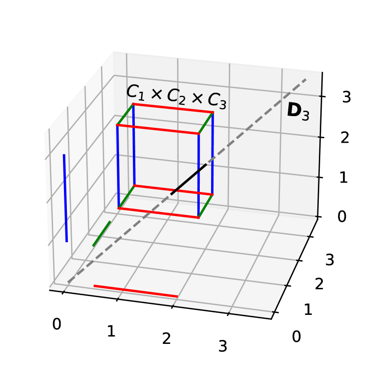
(a) Standard product space reformulation

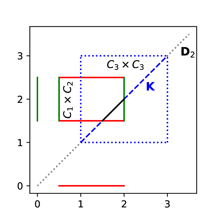
(b) Product space reformulation with reduced dimension

Figure 1: Product space reformulations of the convex feasibility problem in Example 4.1.

Although the theory of projection algorithms is developed under convexity assumptions of the constraint sets, some of them has been shown to be very efficient solvers in a wide variety of nonconvex applications. In special, the Douglas–Rachford algorithm has attracted particular attention due to its well behavior on nonconvex scenarios including some of combinatorial nature; see, e.g., [5, 7, 9, 10, 11, 15, 27, 28, 29, 32]. In most of these applications, feasibility problems are described by more than two sets and need to be tackled by Pierra’s product space reformulation. Indeed, as we recall in the next result, the reformulation is still valid under the more general assumption that the sets are proximinal but not necessarily convex.

Proposition 4.2 (Standard product space reformulation for not necessarily convex feasibility and best approximation problems).

Let $C_{1},C_{2},\ldots,C_{r}\subseteq\mathcal{H}$ be nonempty and proximinal sets and define the product set

$$\boldsymbol{C}=C_{1}\times C_{2}\times\cdots\times C_{r}\subseteq\mathcal{H}^{r}.$$ (4.7)

Then the following hold.

1. $\boldsymbol{C}$ is proximinal and

   $$P_{\boldsymbol{C}}(\boldsymbol{x})=P_{C_{1}}(x_{1})\times P_{C_{2}}(x_{2})\times\cdots\times P_{C_{r}}(x_{r}),\quad\forall\boldsymbol{x}=(x_{1},x_{2},\ldots,x_{r})\in\mathcal{H}^{r}.$$

   If, in addition, $C_{1},C_{2},\ldots,C_{r}$ are closed and convex then so is $\boldsymbol{C}$.

2. $\boldsymbol{D}_{r}$ is a closed subspace with

   $$P_{\boldsymbol{D}_{r}}(\boldsymbol{x})=\boldsymbol{j}_{r}\left(\frac{1}{r}\sum_{i=1}^{r}x_{i}\right),\quad\forall\boldsymbol{x}=(x_{1},x_{2},\ldots,x_{r})\in\mathcal{H}^{r}.$$

3. $\boldsymbol{C}\cap\boldsymbol{D}_{r}=\boldsymbol{j}_{r}\left(\cap_{i=1}^{r}C_{i}\right)$.

4. $P_{\boldsymbol{C}\cap\boldsymbol{D}_{r}}(\boldsymbol{x})=\boldsymbol{j}_{r}\left(P_{\cap_{i=1}^{r}C_{i}}(x)\right),\quad\forall\boldsymbol{x}=\boldsymbol{j}_{r}(x)\in\boldsymbol{D}_{r}$.

Proof.

(i): Let $\boldsymbol{x}=(x_{1},x_{2},\ldots,x_{r})\in\mathcal{H}^{r}$. By direct computations on the definition of projector we obtain that

$$P_{\boldsymbol{C}}(\boldsymbol{x}) =\operatorname*{argmin}_{\boldsymbol{c}\in\boldsymbol{C}}\|\boldsymbol{x}-\boldsymbol{c}\|^{2}=\operatorname*{argmin}_{(c_{1},c_{2},\ldots,c_{r})\in\boldsymbol{C}}\sum_{i=1}^{r}\|x_{i}-c_{i}\|^{2}$$

$$=\operatorname*{argmin}_{c_{1}\in C_{1}}\|x_{1}-c_{1}\|^{2}\times\operatorname*{argmin}_{c_{2}\in C_{2}}\|x_{2}-c_{2}\|^{2}\times\cdots\times\operatorname*{argmin}_{c_{r}\in C_{r}}\|x_{r}-c_{r}\|^{2}$$

$$=P_{C_{1}}(x_{1})\times P_{C_{2}}(x_{2})\times\cdots\times P_{C_{r}}(x_{r}).$$

The remaining assertion easily follows from the definition of (topological) product space.

(ii): Follows from Fact 3.1(ii).

(iii): Let $\boldsymbol{x}\in\boldsymbol{C}\cap\boldsymbol{D}_{r}$. Then $\boldsymbol{x}=\boldsymbol{j}_{r}(x)\in\boldsymbol{D}_{r}$ with $x\in C_{i}$ for all $i=1,2,\ldots,r$. The reverse inclusion is also straightforward.

(iv): Let $\boldsymbol{x}=\boldsymbol{j}_{r}(x)\in\boldsymbol{D}_{r}$. Reasoning as in (i) and taking into account (iii) we get that

$$P_{\boldsymbol{C}\cap\boldsymbol{D}_{r}}(\boldsymbol{x}) =\operatorname*{argmin}_{\boldsymbol{c}\in\boldsymbol{C}\cap\boldsymbol{D}_{r}}\|\boldsymbol{x}-\boldsymbol{c}\|=\boldsymbol{j}_{r}\left(\operatorname*{argmin}_{c\in\cap_{i=1}^{r}C_{i}}\|x-c\|\right)=\boldsymbol{j}_{r}\left(P_{\cap_{i=1}^{r}C_{i}}(x)\right).\qed$$

Analogously, we show the validity of the product space reformulation with reduced dimension for feasibility and best approximation problems with arbitrary proximinal sets.

Proposition 4.3 (Product space reformulation with reduced dimension for non necessarily convex feasibility and best approximation problems).

Let $\allowbreak C_{1},C_{2},\ldots,$ $C_{r}\subseteq\mathcal{H}$ be nonempty and proximinal sets and define

$$\boldsymbol{B}:= C_{1}\times\cdots\times C_{r-1}\subseteq\mathcal{H}^{r-1},$$ (4.8a)

$$\boldsymbol{K}:= \{(x,\ldots,x)\in\mathcal{H}^{r-1}:x\in C_{r}\}\subseteq\mathcal{H}^{r-1}.$$ (4.8b)

Then the following hold.

1. $\boldsymbol{B}$ is proximinal and

   $$P_{\boldsymbol{B}}(\boldsymbol{x})=P_{C_{1}}(x_{1})\times\cdots\times P_{C_{r-1}}(x_{r-1}),\quad\forall\boldsymbol{x}=(x_{1},\ldots,x_{r-1})\in\mathcal{H}^{r-1}.$$

   If, in addition, $C_{1},\ldots,C_{r-1}$ are closed and convex then so is $\boldsymbol{B}$.

2. $\boldsymbol{K}$ is proximinal and

   $$P_{\boldsymbol{K}}(\boldsymbol{x})=\boldsymbol{j}_{r-1}\left(P_{C_{r}}\left(\frac{1}{r-1}\sum_{i=1}^{r}x_{i}\right)\right),\quad\forall\boldsymbol{x}=(x_{1},\ldots,x_{r-1})\in\mathcal{H}^{r-1}.$$

   If, in addition, $C_{r}$ is closed and convex then so is $\boldsymbol{K}$.

3. $\boldsymbol{B}\cap\boldsymbol{K}=\boldsymbol{j}_{r-1}\left(\cap_{i=1}^{r}C_{i}\right)$.

4. $P_{\boldsymbol{B}\cap\boldsymbol{K}}(\boldsymbol{x})=\boldsymbol{j}_{r-1}\left(P_{\cap_{i=1}^{r}C_{i}}(x)\right),\quad\forall\boldsymbol{x}=\boldsymbol{j}_{r-1}(x)\in\boldsymbol{D}_{r-1}$.

Proof.

(i): Follows from Proposition 4.2(i).

(ii): First, let us rewrite

$$\boldsymbol{K}=\boldsymbol{j}_{r-1}(C_{r})=C_{r}^{\,r-1}\cap\boldsymbol{D}_{r-1}=(C_{r}\times\stackrel{{\scriptstyle(r-1)}}{{\cdots}}\times C_{r})\cap\boldsymbol{D}_{r-1}\subseteq\mathcal{H}^{r-1}.$$

Fix $\boldsymbol{x}=(x_{1},\ldots,x_{r-1})\in\mathcal{H}^{r-1}.$ By Proposition 4.2(i) and (ii), $C_{r}^{r-1}$ is a proximinal set and $\boldsymbol{D}_{r-1}$ is a closed subspace with

$$P_{C_{r}^{r-1}}(\boldsymbol{x})=P_{C_{r}}(x_{1})\times\cdots\times P_{C_{r}}(x_{r-1})\quad\text{and}\quad P_{\boldsymbol{D}_{r-1}}(\boldsymbol{x})=\boldsymbol{j}_{r-1}\left(\frac{1}{r-1}\sum_{i=1}^{r-1}x_{i}\right).$$

Observe that, for any arbitrary point $\boldsymbol{y}=\boldsymbol{j}_{r-1}(y)\in\boldsymbol{D}_{r-1}$, it holds that

$$\boldsymbol{j}_{r-1}(p)\in P_{C_{r}^{r-1}}(\boldsymbol{y})\cap\boldsymbol{D}_{r-1},\quad\forall p\in P_{C_{r}}(y).$$

In particular, $P_{C_{r}^{r-1}}(\boldsymbol{y})\cap\boldsymbol{D}_{r-1}\neq\emptyset$ for all $\boldsymbol{y}\in\boldsymbol{D}_{r-1}$. Hence, by applying Lemma 2.9 we derive that

$$P_{\boldsymbol{K}}(\boldsymbol{x}) =P_{C_{r}^{r-1}\cap\boldsymbol{D}_{r-1}}(\boldsymbol{x})=P_{C_{r}^{r-1}}\left(P_{\boldsymbol{D}_{r-1}}(\boldsymbol{x})\right)\cap\boldsymbol{D}_{r-1}$$

$$=P_{C_{r}^{r-1}}\left(\boldsymbol{j}_{r-1}\left(\frac{1}{r-1}\sum_{i=1}^{r-1}x_{i}\right)\right)\cap\boldsymbol{D}_{r-1}=\boldsymbol{j}_{r-1}\left(P_{C_{r}}\left(\frac{1}{r-1}\sum_{i=1}^{r}x_{i}\right)\right).$$

In addition, if $C_{r}$ is closed and convex then so is $C_{r}^{r-1}$ according to Proposition 4.2(i). Since $\boldsymbol{D}_{r-1}$ is a closed subspace, the convexity and closedness of $\boldsymbol{K}$ follows.

(iii) and (iv): Their proofs are straightforward and analogous to the proofs of Proposition 4.2(iii) and (iv), respectively, so they are omitted. ∎

Example 4.4 (Nonconvex feasibility problem).

Consider the feasibility problem

$$\text{Find }x\in C_{1}\cap C_{2}\cap\widehat{C}_{3}\subseteq\mathbb{R},$$ (4.9)

where $C_{1}:=[0.5,2]$, $C_{2}:=[1.5,2]$ and $\widehat{C}_{3}:=\{1,2,3\}$; that is, the problem considered in Example 4.1 but replacing $C_{3}$ by the nonconvex set $\widehat{C}_{3}$. According to Propositions 4.2 and 4.3, the product space reformulations in (4.4) and (4.5), with $C_{3}$ replaced by $\widehat{C}_{3}$, are still valid to reconvert (4.9) into an equivalent problem described by two sets. Both formulations are illustrated in Figure 2, where now we denote

$$\widehat{\boldsymbol{K}}=\{(x,x):x\in\widehat{C}_{3}\}=(\widehat{C}_{3}\times\widehat{C}_{3})\cap\boldsymbol{D}_{2}=\{(1,1),(2,2),(3,3)\}.$$

Due to the nonconvexity, the projector onto $\widehat{C}_{3}$ may be set-valued. In view of Proposition 4.3(ii), the projector onto $\widehat{\boldsymbol{K}}$ is described by

$$P_{\widehat{\boldsymbol{K}}}(x_{1},x_{2})=\left\{(p,p):p\in P_{\widehat{C}_{3}}\left(\frac{x_{1}+x_{2}}{2}\right)\right\}.$$

We emphasize that, in contrast to (4.6b), in the nonconvex case $P_{\widehat{\boldsymbol{K}}}\neq P_{\widehat{C}_{3}\times\widehat{C}_{3}}\circ P_{\boldsymbol{D}_{2}}$. Indeed, consider for instance the point $\boldsymbol{x}:=(2,1)\in\mathbb{R}^{2}$. Then,

$$P_{\widehat{\boldsymbol{K}}}(\boldsymbol{x}) =\{(1,1),(2,2)\},$$

$$P_{\widehat{C}_{3}\times\widehat{C}_{3}}(P_{\boldsymbol{D}_{2}}(\boldsymbol{x})) =P_{\widehat{C}_{3}\times\widehat{C}_{3}}((1.5,1.5))=\{(1,1),(1,2),(2,1),(2,2)\}.$$

Therefore, $P_{\widehat{C}_{3}\times\widehat{C}_{3}}(P_{\boldsymbol{D}_{2}}(\boldsymbol{x}))\neq P_{\widehat{\boldsymbol{K}}}(\boldsymbol{x})=P_{\widehat{C}_{3}\times\widehat{C}_{3}}(P_{\boldsymbol{D}_{2}}(\boldsymbol{x}))\cap\boldsymbol{D}_{2}$.

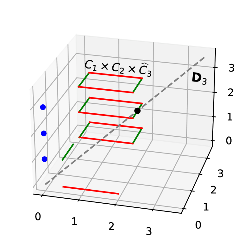
(a) Standard product space reformulation

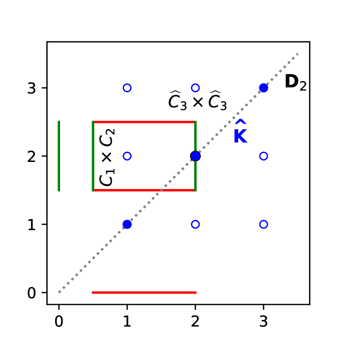
(b) Product space reformulation with reduced dimension

Figure 2: Product space reformulations of the nonconvex feasibility problem in Example 4.4.

5 Application to splitting algorithms

In this section, we apply our proposed reformulation in Theorem 3.3 in order to derive two new parallel splitting algorithms, one for solving problem (1.1), and another one for (1.2). In the first case, we consider the Douglas–Rachford (DR) algorithm [26, 33] (see also [16, 17] for recent results in the inconsistent case). The DR algorithm permits to find a zero of the sum of two maximally monotone operators. When it is applied to Pierra’s standard reformulation the resulting method takes the form in [14, Proposition 26.12]. In contrast, if the problem is reformulated via Theorem 3.3 we obtain the following iterative scheme, which requires one variable less.

Theorem 5.1 (Parallel Douglas/Peaceman–Rachford splitting algorithm).

Let $\allowbreak A_{1},A_{2},\ldots,A_{r}:\mathcal{H}\rightrightarrows\mathcal{H}$ be maximally monotone operators such that $\operatorname{zer}(\sum_{i=1}^{r}A_{i})\neq\emptyset$. Let $\gamma>0$ and let $\lambda\in{]}0,2]$. Given $x_{1,0},\ldots,x_{r-1,0}\in\mathcal{H}$, set

$$\text{for }k=0,1,2,\ldots:$$ (5.1)

$$\left\lfloor\begin{array}[]{l}p_{k}=J_{\frac{\gamma}{r-1}A_{r}}\left(\frac{1}{r-1}\sum_{i=1}^{r-1}x_{i,k}\right),\\ \text{for }i=1,2,\ldots,r-1:\\ \left\lfloor\begin{array}[]{l}z_{i,k}=J_{\gamma A_{i}}\left(2p_{k}-x_{i,k}\right),\\ x_{i,k+1}=x_{i,k}+\lambda\left(z_{i,k}-p_{k}\right).\end{array}\right.\end{array}\right.$$

Then the following hold.

1. If $\lambda\in{]0,2[}$, then $p_{k}\rightharpoonup p^{\star}$ and $z_{i,k}\rightharpoonup p^{\star}$, for $i=1,\ldots,r-1$, with $p^{\star}\in\operatorname{zer}(\sum_{i=1}^{r}A_{i})$.

2. If $A_{r}$ is uniformly monotone, then $p_{k}\to p^{\star}$ and $z_{i,k}\to p^{\star}$, for $i=1,\ldots,r-1$, where $p^{\star}$ is the unique point in $\operatorname{zer}(\sum_{i=1}^{r}A_{i})$.

Proof.

Consider the product Hilbert space $\mathcal{H}^{r-1}$ and let $\boldsymbol{B},\boldsymbol{K}:\mathcal{H}^{r-1}\rightrightarrows\mathcal{H}^{r-1}$ be the operators defined in (3.2). By Theorem 3.3(i), (ii) and (iii), we get that $\boldsymbol{B}$ and $\boldsymbol{K}$ are maximally monotone with $\operatorname{zer}(\boldsymbol{B}+\boldsymbol{K})=\boldsymbol{j}_{r-1}(\operatorname{zer}(\sum_{i=1}^{r}A_{i}))\neq\emptyset$. For each $k=0,1,2,\ldots$, set $\boldsymbol{x}_{k}:=(x_{1,k},\ldots,x_{r-1,k}),\boldsymbol{z}_{k}:=(z_{1,k},\ldots,z_{r-1,k})\in\mathcal{H}^{r-1}$ and $\boldsymbol{p}_{k}=\boldsymbol{j}_{r-1}(p_{k})\in\boldsymbol{D}_{r-1}$. Hence, according to Theorem 3.3(i) and (ii), we can rewrite (5.1) as

$$\text{for }k=0,1,2,\ldots:$$ (5.2)

$$\left\lfloor\begin{array}[]{l}\boldsymbol{p}_{k}=J_{\gamma\boldsymbol{K}}(\boldsymbol{x}_{k}),\\ \boldsymbol{z}_{k}=J_{\gamma\boldsymbol{B}}\left(2\boldsymbol{p}_{k}-\boldsymbol{x}_{k}\right),\\ \boldsymbol{x}_{k+1}=\boldsymbol{x}_{k}+\lambda\left(\boldsymbol{z}_{k}-\boldsymbol{p}_{k}\right).\end{array}\right.$$

Note that (5.2) is the Douglas–Rachford (or Peaceman–Rachford) iteration applied to the operators $\boldsymbol{B}$ and $\boldsymbol{K}$. If $\lambda\in{]0,2[}$, we apply [14, Theorem 26.11(iii)] to obtain that $\boldsymbol{p}_{k}\rightharpoonup\boldsymbol{p}^{\star}$ and $\boldsymbol{z}_{k}\rightharpoonup\boldsymbol{p}^{\star}$, with $\boldsymbol{p}^{\star}\in\operatorname{zer}(\boldsymbol{B}+\boldsymbol{K})$. Hence, $\boldsymbol{p}^{\star}=\boldsymbol{j}_{r-1}(p^{\star})$ with $p^{\star}\in\operatorname{zer}\left(\sum_{i=1}^{r}A_{i}\right)$, which implies (i).

Suppose in addition that $A_{r}$ is uniformly monotone. Then so is $\boldsymbol{K}$ according to Theorem 3.3(ii). Hence, (ii) follows from [14, Theorem 26.11(vi)], when $\lambda\in{]0,2[}$, and [14, Proposition 26.13] when $\lambda=2$. ∎

Remark 5.2 (Frugal resolvent splitting algorithms with minimal lifting).

Consider the problem of finding a zero of the sum of three maximally monotone operators $A,B,C:\mathcal{H}\rightrightarrows\mathcal{H}$. The classical procedure to solve it has been to employ the standard product space reformulation (Fact 3.1) to construct a DR algorithm on $\mathcal{H}^{3}$. The question of whether it is possible to generalize the DR algorithm to three operators without lifting, that is, without enlarging the ambient space, was solved with a negative answer by Ryu in [43]. The generalization is considered in the sense of devising a frugal splitting algorithm which uses the resolvent of each operator exactly once per iteration. In the same work, the author demonstrated that the minimal lifting is $2$-fold (in $\mathcal{H}^{2}$) by providing the following splitting algorithm. Given $\lambda\in{]0,1[}$ and $x_{0},y_{0}\in\mathcal{H}$, set

$$\text{for }k=0,1,2,\ldots:$$ (5.3)

$$\left\lfloor\begin{array}[]{l}u_{k}=J_{\gamma A}(x_{k})\\ v_{k}=J_{\gamma B}(u_{k}+y_{k})\\ w_{k}=J_{\gamma C}(u_{k}-x_{k}+v_{k}-y_{k})\\ x_{k+1}=x_{k}+\lambda(w_{k}-u_{k})\\ y_{k+1}=y_{k}+\lambda(w_{k}-v_{k}).\end{array}\right.$$

Then $u_{k}\rightharpoonup w^{\star}$, $v_{k}\rightharpoonup w^{\star}$ and $w_{k}\rightharpoonup w^{\star}$, with $w^{\star}\in\operatorname{zer}(A+B+C)$ (see [43, Theorem 4] or [12, Appendix A] for an alternative proof in an infinite-dimensional space).

A few days after the publication of the first preprint version of this manuscript (ArXiv: 2107.12355), Malitsky and Tam [35] generalized Ryu’s result by showing that for an arbitrary number of $r$ operators the minimal lifting is $(r-1)$-fold. In addition, they proposed another frugal splitting algorithm that attains this minimal lifting, whose iteration is described as follows. Given $\lambda\in{]0,1[}$ and $\boldsymbol{z}_{0}=(z_{1,0},\ldots,z_{r-1,0})\in\mathcal{H}^{r-1}$, set

$$\text{for }k=0,1,2,\ldots:$$ (5.4)

$$\left\lfloor\begin{array}[]{l}\text{Compute }\boldsymbol{z}_{k+1}=(z_{1,k+1},\ldots,z_{r-1,k+1})\in\mathcal{H}^{r-1}\text{ as }\\ \boldsymbol{z}_{k+1}=\boldsymbol{z}_{k}+\lambda\left(\begin{array}[]{c}x_{2,k}-x_{1,k}\\ x_{3,k}-x_{2,k}\\ \vdots\\ x_{r,k}-x_{r-1,k}\end{array}\right),\\ \text{where }\boldsymbol{x}_{k}=(x_{1,k},x_{2,k},\ldots,x_{r,k})\in\mathcal{H}^{r}\text{ is given by }\\ \hskip 8.61108ptx_{1,k}=J_{\gamma A_{1}}(z_{1,k}),\\ \hskip 8.61108pt\text{for }k=2,\ldots,r-1:\\ \hskip 8.61108pt\left\lfloor\begin{array}[]{l}\hskip 8.61108ptx_{i,k}=J_{\gamma A_{i}}(z_{i,k}-z_{i-1,k}+x_{i-1,k}),\end{array}\right.\\ \hskip 8.61108ptx_{r,k}=J_{\gamma A_{r}}(x_{1,k}+x_{r-1,k}-z_{r-1,k}).\end{array}\right.$$

Then, for each $i\in\{1,\ldots,r\}$, $x_{i,k}\rightharpoonup x^{*}\in\operatorname{zer}(\sum_{j=1}^{r}A_{j})$ (see [35, Theorem 4.5]).

It is worth to notice that the Malitsky–Tam iteration (5.4) does not generalize Ryu’s scheme (5.3), which seems to be difficult to extend to more than three operators as explained in [35, Remark 4.7]. Furthermore, both of these algorithms are different from the one in Theorem 5.1. The main conceptual difference is that (5.4) can be implemented in a distributed decentralized way whereas algorithm (5.1) uses the operator $A_{r}$ as a central coordinator (see [35, § 5]). Nevertheless, for the applications considered in this work, the dimensionality reduction obtained through the new product space reformulation seems to be more effective for accelerating the converge of the algorithm, especially when the number of operators is large as we shall show in Section 6.

We now turn our attention into splitting algorithms for problem (1.2). In particular, we concern on the averaged alternating modified reflections (AAMR) algorithm, originally proposed in [6] for best approximation problems, and later extended in [8] for monotone operators (see also [3, 12]). The parallel AAMR splitting iteration obtained from Pierra’s reformulation is given in [8, Theorem 4.1]. As we show in the following result, we can avoid one of the variables defining the iterative scheme if we use the product space reformulation in Theorem 3.3.

Theorem 5.3 (Parallel AAMR splitting algorithm).

Let $\allowbreak A_{1},A_{2},\ldots,A_{r}:\mathcal{H}\rightrightarrows\mathcal{H}$ be maximally monotone operators, let $\gamma>0$ and let $\lambda\in{]0,2]}$. Let $\beta\in{]0,1[}$ and suppose that $q\in\operatorname{ran}\left(\operatorname{Id}+\frac{\gamma}{2(1-\beta)(r-1)}\sum_{i=1}^{r}A_{i}\right)$. Given $x_{1,0},\ldots,x_{r-1,0}\in\mathcal{H}$, set

$$\text{for }k=0,1,2,\ldots:$$ (5.5)

$$\left\lfloor\begin{array}[]{l}p_{k}=J_{\frac{\gamma}{r-1}A_{r}}\left(\frac{\beta}{r-1}\sum_{i=1}^{r-1}x_{i,k}+(1-\beta)q\right),\\ \text{for }i=1,2,\ldots,r-1:\\ \left\lfloor\begin{array}[]{l}z_{i,k}=J_{\gamma A_{i}}\left(\beta(2p_{k}-x_{i,k})+(1-\beta)q\right),\\ x_{i,k+1}=x_{i,k}+\lambda\left(z_{i,k}-p_{k}\right).\end{array}\right.\end{array}\right.$$

Then $\left(p_{k}\right)_{k=0}^{\infty}$ converges strongly to $J_{\frac{\gamma}{2(1-\beta)(r-1)}\sum_{i=1}^{r}A_{i}}(q)$.

Proof.

Consider the product Hilbert space $\mathcal{H}^{r-1}$ and let $\boldsymbol{B},\boldsymbol{K}:\mathcal{H}^{r-1}\rightrightarrows\mathcal{H}^{r-1}$ be the operators defined in (3.2). We know that $\boldsymbol{B}$ and $\boldsymbol{K}$ are maximally monotone by Theorem 3.3(i) and (ii), respectively. Set $\boldsymbol{x}_{k}:=(x_{1,k},\ldots,x_{r-1,k}),\boldsymbol{z}_{k}:=(z_{1,k},\ldots,z_{r-1,k})\in\mathcal{H}^{r}$ and $\boldsymbol{p}_{k}=\boldsymbol{j}_{r-1}(p_{k})\in\boldsymbol{D}_{r-1}$, for each $k=0,1,2,\ldots$, and set $\boldsymbol{q}:=\boldsymbol{j}_{r-1}(q)\in\boldsymbol{D}_{r-1}$. On the one hand, according to Theorem 3.3(i) and (ii), we can rewrite (5.5) as

$$\text{for }k=0,1,2,\ldots:$$

$$\left\lfloor\begin{array}[]{l}\boldsymbol{p}_{k}=J_{\gamma\boldsymbol{K}}\left(\beta\boldsymbol{x}_{k}+(1-\beta)\boldsymbol{q}\right)\\ \boldsymbol{z}_{k}=J_{\gamma\boldsymbol{B}}\left(\beta(2\boldsymbol{p}_{k}-\boldsymbol{x}_{k})+(1-\beta)\boldsymbol{q}\right)\\ \boldsymbol{x}_{k+1}=\boldsymbol{x}_{k}+{\lambda}(\boldsymbol{z}_{k}-\boldsymbol{p}_{k}).\end{array}\right.$$

On the other hand, from Theorem 3.3(iv) we obtain that

$$J_{\frac{\gamma}{2(1-\beta)}(\boldsymbol{B}+\boldsymbol{K})}(\boldsymbol{q})=\boldsymbol{j}_{r-1}\left(J_{\frac{\gamma}{2(1-\beta)(r-1)}\sum_{i=1}^{r}A_{i}}\left(q\right)\right).$$

In particular, the latter implies that $\boldsymbol{q}\in\operatorname{ran}\left(\operatorname{Id}+\frac{\gamma}{2(1-\beta)}(\boldsymbol{B}+\boldsymbol{K})\right)$. Hence, by applying [12, Theorem 6 and Remark 10(i)], we conclude that $\left(\boldsymbol{p}_{k}\right)_{k=0}^{\infty}$ converges strongly to $J_{\frac{\gamma}{2(1-\beta)}(\boldsymbol{B}+\boldsymbol{K})}(\boldsymbol{q})$ and the result follows. ∎

Remark 5.4 (On Forward-Backward type methods).

Forward-Backward type methods permit to find a zero in $A+B$ when $A:\mathcal{H}\to\mathcal{H}$ is cocoercive (see, e.g., [14, Theorem 26.14]) or Lipschitz continuous (see, e.g., [19, 34, 44]) and $B:\mathcal{H}\rightrightarrows\mathcal{H}$ is maximally monotone. These algorithms make use of direct evaluations of $A$ (forward steps) and resolvent computations of $B$ (backward steps). When dealing with finitely many operators of both nature (single-valued and set-valued), Pierra’s reformulation (Fact 3.1) yields parallel algorithms which need to activate all of them through their resolvents, since all of them are combined into the product operator $\boldsymbol{A}$ in (3.1). In contrast, the product space reformulation in Theorem 3.3 allows to deal with the case when $A_{1},\ldots,A_{r-1}:\mathcal{H}\to\mathcal{H}$ are cocoercive/Lipschitz continuous and $A_{r}:\mathcal{H}\rightrightarrows\mathcal{H}$ is maximally monotone. Indeed, it can be easily proved that the product operator $\boldsymbol{B}$ in (3.2a) keeps the cocoercivity/Lipschitz continuity property. However, the parallel algorithm obtained with this approach will coincide with the original Forward-Backward type algorithm applied to the operators $\sum_{i=1}^{r-1}A_{i}$ and $A_{r}$. It is worth mentioning that in the opposite case, that is, when one operator is cocoercive and the remaining ones are maximally monotone, a parallel Forward-Backward algorithm was developed in [40].

6 Numerical experiments

In this section, we perform some numerical experiments to assess the advantage of the new proposed reformulation when applied to splitting or projection algorithms. In particular, we compare the performance of the proposed parallel Douglas–Rachford algorithm in Theorem 5.1 with the standard parallel version in [14, Proposition 26.12], first on a convex minimization problem and then in a nonconvex feasibility problem. We will refer to these algorithms as Reduced-DR and Standard-DR, respectively. In some experiments we will also test the algorithms in [43, Theorem 4] and [35, Theorem 4.5], wich will be referred to as Ryu and Malitsky–Tam, respectively. All codes were written in Python 3.7 and the tests were run on an Intel Core i7-10700K CPU 3.80GHz with 64GB RAM, under Ubuntu 20.04.2 LTS (64-bit).

6.1 The generalized Heron problem

We first consider the generalized Heron problem, which is described as follows. Given $\Omega_{1},\ldots,\Omega_{r}\subseteq\mathbb{R}^{n}$ nonempty, closed and convex sets, we are interested in finding a point in $\Omega_{r}$ that minimizes the sum of the distances to the remaining sets; that is,

$$\begin{array}[]{rl}\text{Min}&\sum_{i=1}^{r-1}d_{\Omega_{i}}(x)\\ \text{s.t.}&x\in\Omega_{r}.\end{array}$$ (6.1)

This problem was investigated with modern convex analysis tools in [36, 37], where it was solved by subgradient-type algorithms. It was later revisited in [18], where the authors implemented their proposed paralellized Douglas–Rachford-type primal-dual methods for its resolution. Indeed, splitting algorithms such as Douglas–Rachford can be employed to solve problem (6.1) as this is equivalent to the monotone inclusion (1.1) with

$$A_{r}=\partial\iota_{\Omega_{r}}=N_{\Omega_{r}}\quad\text{and}\quad A_{i}=\partial d_{\Omega_{i}},\text{ for }i=1,\ldots,r-1.$$

According to Facts 2.6 and 2.8, $J_{\gamma A_{r}}=P_{\Omega_{r}}$ and $J_{\gamma A_{i}}=\operatorname{prox}_{\gamma d_{\Omega_{i}}}$, for $i=1,\ldots,r-1$. We recall that the proximity operator of the distance function to a closed and convex set $C\subseteq\mathcal{H}$ is given by

$$\operatorname{prox}_{\gamma d_{C}}(x)=\left\{\begin{array}[]{ll}x+\frac{\gamma}{{d_{C}(x)}}\left({P_{C}(x)-x}\right),&\text{if }d_{C}(x)>\gamma,\\ P_{C}(x),&\text{otherwise}.\end{array}\right.$$

In our experiments, the constraint sets $\Omega_{1},\ldots,\Omega_{r-1}$ in (6.1) were randomly generated hypercubes of centers $(c_{i,1},\ldots,c_{i,n}),\ldots,(c_{r-1,1},\ldots,c_{r-1,n})\in\mathbb{R}^{n}$ with length side $\sqrt{2}$, while $\Omega_{r}$ was chosen to be the closed ball centered at zero with radius $10$; that is,

$$\Omega_{i} :=\left\{(x_{1},\ldots,x_{n})\in\mathbb{R}^{n}:|c_{i,j}-x_{j}|\leq\frac{\sqrt{2}}{2},\,j=1,\ldots,n\right\},\quad i=1,\ldots,r-1,$$ (6.2a)

$$\Omega_{r} :=\{x\in\mathbb{R}^{n}:\|x\|\leq 10\}.$$ (6.2b)

More precisely, the centers of the hypercubes were randomly generated with norm greater or equal than $12$, so that the hypercubes did not intersect the ball. Two instances of the problem with $r=5$, in $\mathbb{R}^{2}$ and $\mathbb{R}^{3}$, are illustrated in Figure 3.

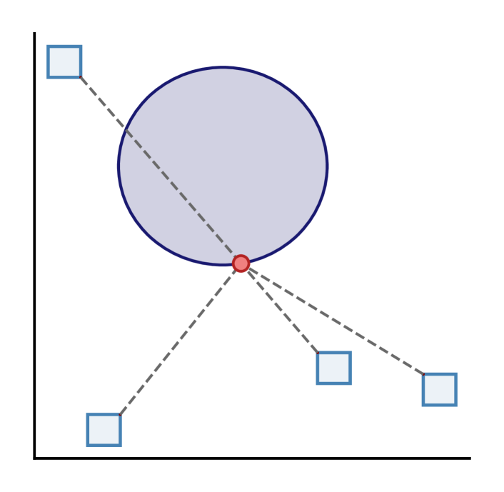
Figure 3: The generalized Heron problem consisting in finding a point in a ball in $\mathbb{R}^{2}$ (left) or $\mathbb{R}^{3}$ (right) that minimizes the sum of the distances to four squares (left) or cubes (right). A solution to the problem is represented by a red point.

In our first numerical test, we generated 10 instances of the problem (6.1)–(6.2) in $\mathbb{R}^{100}$ with $r=3$. For each $\gamma\in\{1,10,25,50,75,100\}$ and each $\lambda\in\{0.1,0.2,\ldots,1.9\}$, Standard-DR and Reduced-DR were run from $10$ random starting points. For those values of $\lambda\leq 1$, Ryu and Malitsky–Tam algorithms were also run from the same initial points. All algorithms were stopped when the monitored sequence $\{p_{k}\}_{k=0}^{\infty}$ verified the Cauchy-type stopping criteria

$$\|p_{k+1}-p_{k}\|<\varepsilon:=10^{-6}$$

for the first time. For a fairer comparison, for each algorithm we monitored that sequence which is projected onto the feasible set $\Omega_{r}$ so that all of them lay on the same ambient space. The average number of iterations required by each algorithm among all problems and starting points is depicted in Figure 4. In Table 1 we list the best results obtained by each algorithm and the value of the parameters at which those results were achieved.

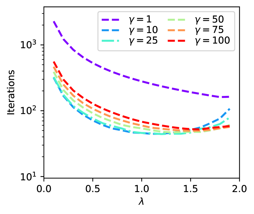
(a) Standard-DR

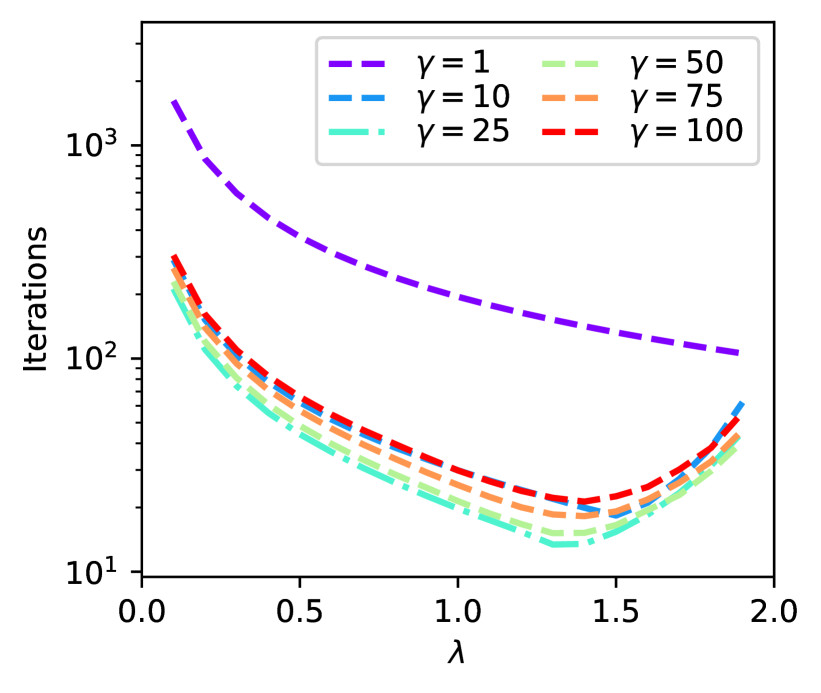
(b) Reduced-DR

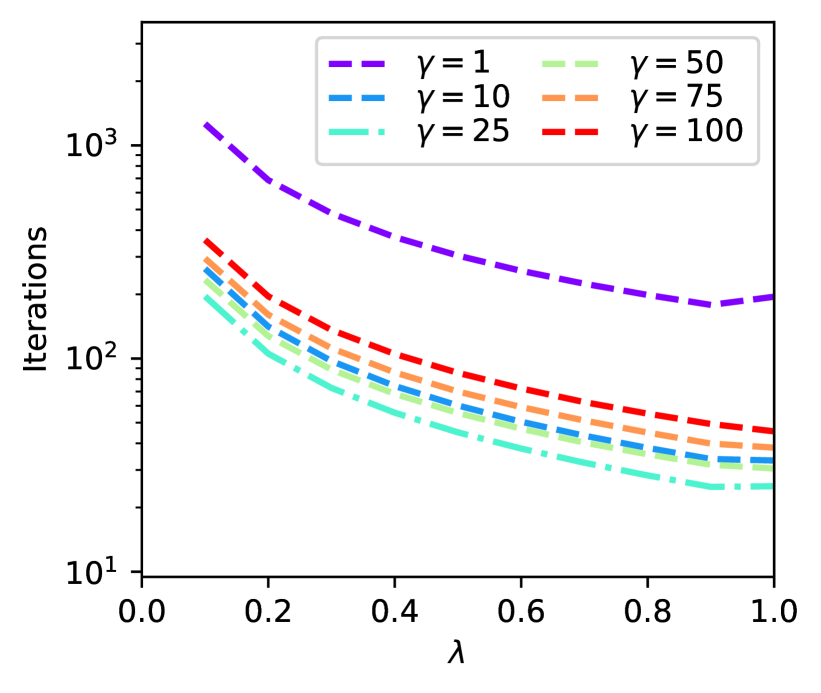
(c) Malitsky–Tam

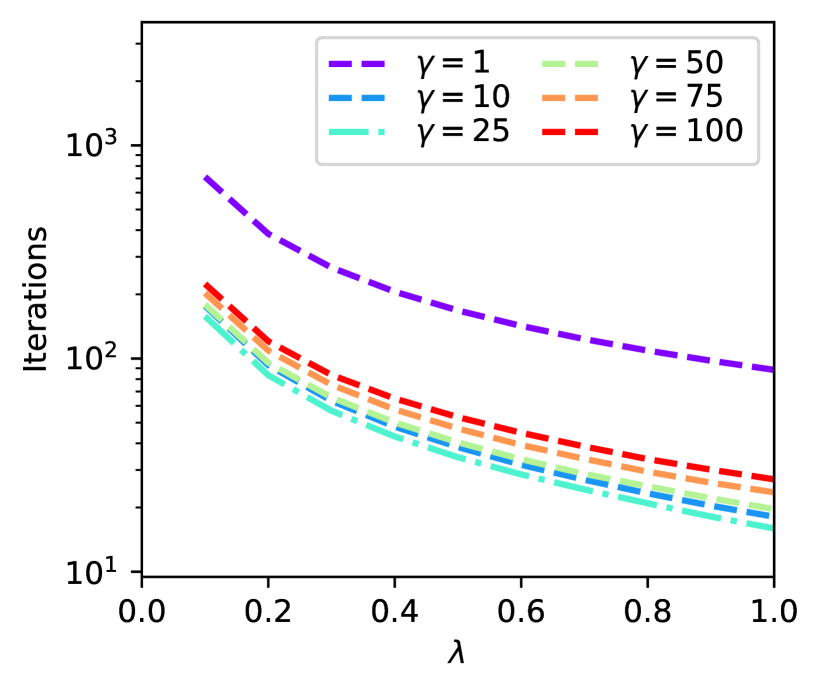
(d) Ryu

Figure 4: Performance of Standard-DR, Reduced-DR, Malitsky–Tam and Ryu algorithms for solving the generalized Heron problem in $\mathbb{R}^{100}$ with $r=3$. For each pair of parameters $(\gamma,\lambda)$, we represent the average number of iterations among $10$ problems and $10$ random starting points each.

Algorithm	$\gamma$	$\lambda$	Average iterations
Standard-DR	$25$	$1.2$	$44.15$
Reduced-DR	$25$	$1.3$	$13.41$
Malitsky–Tam	$25$	$0.9$	$25.00$
Ryu	$25$	$1.0$	$15.96$

Table 1: Best choice of parameters and minimum averaged number of iterations, among $10$ problems and $10$ random starting points each, required by Standard-DR, Reduced-DR, Malitsky–Tam and Ryu algorithms for solving the generalized Heron problem in $\mathbb{R}^{100}$ with $r=3$.

Once the parameters had been tuned, we analyzed the effect of the dimension of the space ($n$), as well as the number of operators ($r$), on the comparison between all algorithms. For the first purpose, we fixed $r=3$ and generated $20$ problems in $\mathbb{R}^{n}$ for each $n\in\{100,200,\ldots,1000\}$. Then, for each problem we computed the average time, among $10$ random starting points, required by each algorithm to converge. Parameters $\gamma$ and $\lambda$ were chosen as in Table 1 according to the previous experiment. The results, shown in Figure 5(a), confirm the consistent advantage of Reduced-DR and Ryu for all sizes. Indeed, these two algorithms were around 4 times faster than Standard-DR, whereas Malitsky–Tam was 2 times faster than Standard-DR.

For the second objective we repeated the experiment where now, for each number of operators $r\in\{3,4,\ldots,20\}$, we generated $20$ problems in $\mathbb{R}^{100}$. We did not consider Ryu splitting algorithm since it is only devised for three operators. We show the results in Figure 5(b), from which we deduce that the superiority of Reduced-DR and Malitsky–Tam over Pierra’s standard reformulation is diminished as the number of operators increases. However, this drop is more drastic for the Makitsky–Tam algorithm. In fact, while Reduced-DR is still always preferable to Standard-DR for all the considered values of $r$, Malitsky–Tam algorithm turns even slower than the classical approach when the number of operators is greater than $6$.

(a) $n\in\{100,200,\ldots,1000\}$ and $r=3$.

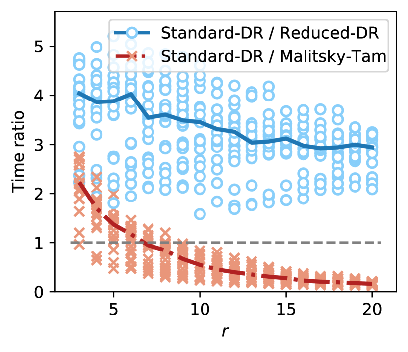
(b) $n=100$ and $r\in\{3,4,\ldots,20\}$.

Figure 5: Comparison of the performance of Standard-DR, Reduced-DR, Malitsky–Tam and Ryu algorithms for solving $20$ instances of generalized Heron problem with $r$ sets in $\mathbb{R}^{n}$ for different values of $n$ and $r$. For each problem we represent the ratio between the average time required by each algorithm over Reduced-DR, among $10$ random starting points. The colored lines connect the median of the ratios while the dashed grey line represents ratios equal to $1$.

6.2 Sudoku puzzles

In this section we analyze the potential of the product space reformulation with reduced dimension for nonconvex feasibility problems (Proposition 4.3). To this aim, we concern on Sudoku puzzles, which were first investigated by the Douglas–Rachford algorithm in [28]. Since then, other formulations as feasibility problems have been studied; see, e.g., [5, 7, 9]. In this paper we consider the formulation with binary variables described in [5, Section 6.2], which we explain next.

Recall that a Sudoku puzzle is defined by a $9\times 9$ grid, composed by nine $3\times 3$ subgrids, where some of the cells are prescribed with some given values. The objective is to fill the remaining cells so that each row, each column and each subgrid contains the digits from $1$ to $9$ exactly once. Possible solutions to a given Sudoku are encoded as a 3-dimensional multiarray $X\in\mathbb{R}^{9\times 9\times 9}$ with binary entries defined componentwise as

$$X[i,j,k]=\left\{\begin{array}[]{cl}1,&\text{if digit }k\text{ is assigned to the }(i,j)\text{th entry of the Sudoku},\\ 0,&\text{otherwise;}\end{array}\right.$$ (6.3)

for $(i,j,k)\in I^{3}$ where $I:=\{1,2,\ldots,9\}$. Let $\mathcal{C}:=\{e_{1},e_{2},\ldots,e_{9}\}$ be the standard basis of $\mathbb{R}^{9}$, let $J\subseteq I^{3}$ be the set of indices for the prescribed entries of the Sudoku, and denote by $\operatorname{vec}M$ the vectorization, by columns, of a matrix $M$. Under encoding (6.3), a solution to the Sudoku can be found by solving the feasibility problem

$$\text{Find }X\in C_{1}\cap C_{2}\cap C_{3}\cap C_{4}\cap C_{5}\subseteq\mathbb{R}^{9\times 9\times 9},$$ (6.4)

where the constraint sets are defined by

$$C_{1} :=\left\{X\in\mathbb{R}^{9\times 9\times 9}:X[i,:,k]\in\mathcal{C},\forall i,k\in I\right\},$$

$$C_{2} :=\left\{X\in\mathbb{R}^{9\times 9\times 9}:X[:,j,k]\in\mathcal{C},\forall j,k\in I\right\},$$

$$C_{3} :=\left\{X\in\mathbb{R}^{9\times 9\times 9}:X[i,j,:]\in\mathcal{C},\forall i,j\in I\right\},$$

$$C_{4} :=\left\{X\in\mathbb{R}^{9\times 9\times 9}:\begin{array}[]{c}\operatorname{vec}X[3i+1:3(i+1),3j+1:3(j+1),k]\in\mathcal{C},\\ \forall i,j\in\{0,1,2\},\forall k\in I\end{array}\right\},$$

$$C_{5} :=\left\{X\in\mathbb{R}^{9\times 9\times 9}:X[i,j,k]=1,\forall(i,j,k)\in J\right\}.$$

Observe that nonconvexity of problem (6.4) arises from the combinatorial structure of $C_{1}$, $C_{2}$, $C_{3}$, $C_{4}\subseteq\{0,1\}^{9\times 9\times 9}$. Projections onto these sets can be computed by means of the projector mapping onto $\mathcal{C}$ (see [5, Remark 5.1]). On the other hand, $C_{5}$ is an affine subspace of $\mathbb{R}^{9\times 9\times 9}$ whose projector can be readily computed component-wise as

$$P_{C_{5}}(X)[i,j,k]=\left\{\begin{array}[]{ll}1,&\text{if }(i,j,k)\in J,\\ X[i,j,k],&\text{otherwise.}\end{array}\right.$$

In our experiment we considered the 95 hard puzzles from the library top95. For each puzzle, we run Standard-DR, Reduced-DR and Malitsky–Tam from $10$ random initial points. Parameter $\lambda$ was roughly tuned for good performance and it was fixed to $\lambda=1$ for Standard-DR and Reduced-DR and $\lambda=0.5$ for Malitsky–Tam. The algorithms were stopped when either they found a solution or when the CPU running time exceeded 5 minutes. A summary of the results can be found in Table 2. While the success of all three algorithms is very similar, the average CPU time and, specially, the proportion of wins are clearly favorable to Reduced-DR.

Algorithm	Solved	Wins	Time (median)
Standard-DR	$91.78\%$	$18.94\%$	$0.7423~{}s.$
Reduced-DR	$91.78\%$	$55.47\%$	$0.5904~{}s.$
Malitsky–Tam	$88.73\%$	$15.05\%$	$0.8836~{}s.$

Table 2: Results of the comparison between Standard-DR, Reduced-DR and Malitsky–Tam algorithm for solving 95 Sudoku problems from $10$ random starting points each. For each algorithm, we show the percentage of solved instances, the percentage of instances for which the algorithm was fastest, and the median of the CPU time required among the solved instances. Instances were labeled as unsolved after 5 minutes.

In order to better visualize the results we turn to performance profiles (see [25] and the modification proposed in [30]), which are constructed as explained next.

Performance profiles

Let $\mathcal{A}$ denote a set of algorithms to be tested on be a set of $N$ problems, denoted by $\mathcal{P}$, for multiple runs (starting points). Let $s_{a,p}$ denote the fraction of successful runs of algorithm $a\in\mathcal{A}$ on problem $p\in\mathcal{P}$ and let $t_{a,p}$ be the averaged time required to solve those successful runs. Compute $t^{\star}_{p}:=\min_{a\in\mathcal{A}}t_{a,p}$ for all $p\in\mathcal{P}$. Then, for any $\tau\geq 1$, define $R_{a}(\tau)$ as the set of problems for which algorithm $a$ was at most $\tau$ times slower than the best algorithm; that is, $R_{a}(\tau):=\{p\in\mathcal{P},t_{a,p}\leq\tau t^{\star}_{p}\}$. The performance profile function of algorithm $a$ is given by

$$\begin{array}[]{rccl}\rho_{a}:&[1,+\infty)&\longmapsto&[0,1]\\ &\tau&\mapsto&\rho_{a}(\tau):=\frac{1}{N}\sum_{p\in R_{a}(\tau)}s_{a,p}.\end{array}$$

The value $\rho_{a}(1)$ indicates the portion of runs for which $f$ was the fastest formulation. When $\tau\rightarrow+\infty$, then $\rho_{a}(\tau)$ gives the proportion of successful runs for formulation $f$.

Performance profiles of the results of Sudoku experiment are shown in Figure 6, which confirm the conclusions drawn from Table 2. Furthermore, we can now asses that Reduced-DR becomes consistently superior since its performance profile is mostly above the one of the remaining two algorithms.

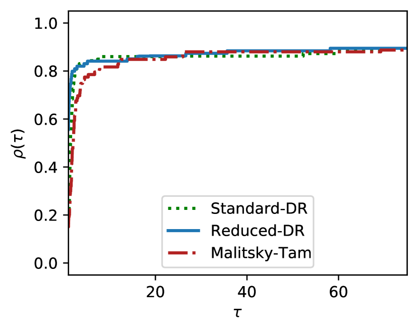
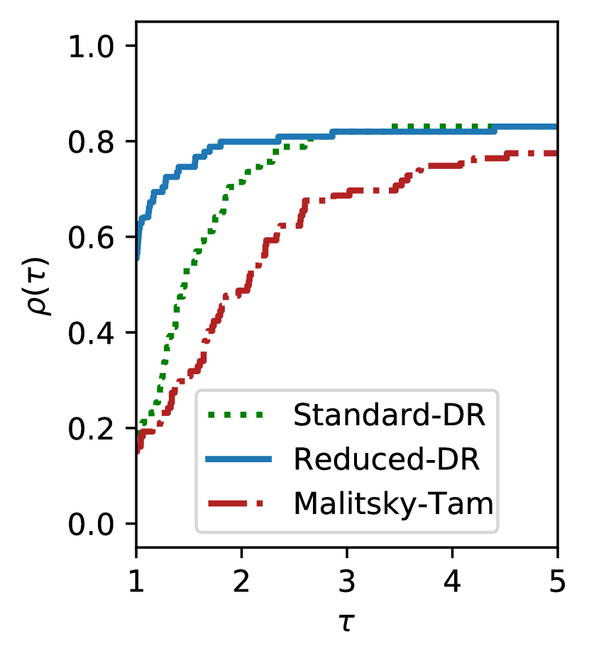
Figure 6: Performance profiles comparing Standard-DR, Reduced-DR and Malitsky–Tam algorithm for solving 95 Sudoku problems (left). For each problem, 10 random starting points were considered. Instances were labeled as unsolved after 5 minutes of CPU running time. For the sake of clarity we focus the view of the performance profiles to the values of $\tau\in[1,5]$ (right).

We would like to conclude with the following comment regarding the implementation of splitting algorithms on (6.4).

Remark 6.1 (On the order of the sets).

Observe that Pierra’s classical reformulation in Proposition 4.2, and thus Standard-DR, is completely symmetric on the order of the sets $C_{1},\ldots,C_{5}$. However, this is not the case for the reformulation in Proposition 4.3, where one has to decide which of the sets will be merged to the diagonal to construct the set $\boldsymbol{K}$ in (4.8b). In our test, we followed the arrangement in Proposition 4.3, that is,

$$\boldsymbol{B}:= C_{1}\times C_{2}\times C_{3}\times C_{4}\subseteq(\mathbb{R}^{9\times 9\times 9})^{4},$$

$$\boldsymbol{K}:= \{(x,x,x,x)\in(\mathbb{R}^{9\times 9\times 9})^{4}:x\in C_{5}\}\subseteq(\mathbb{R}^{9\times 9\times 9})^{4}.$$

Note that this makes the constrained diagonal set $\boldsymbol{K}$ to be an affine subspace. Due to the nonconvexity of the problem, the reformulation chosen may be crucial for the success of the algorithm. For example, we tested all the remaining combinations, for which Reduced-DR rarely found a solution on the considered problems within the first 5 minutes of running time.

Acknowledgements

The author was partially supported by the Ministry of Science, Innovation and Universities of Spain and the European Regional Development Fund (ERDF) of the European Commission (PGC2018-097960-B-C22), and by the Generalitat Valenciana (AICO/2021/165).

References

• [1]
• [2] Adly, S., Bourdin, L.: On a decomposition formula for the resolvent operator of the sum of two set-valued maps with monotonicity assumptions. Appl. Math. Opt. 80(3), 715–732 (2019)
• [3] Alwadani, S., Bauschke, H. H., Moursi, W. M., & Wang, X. On the asymptotic behaviour of the Aragón Artacho–Campoy algorithm. Oper. Res. Lett. 46(6), 585–587 (2018)
• [4] Aragón Artacho, F.J., Borwein, J.M., Tam, M.K.: Douglas–Rachford feasibility methods for matrix completion problems. ANZIAM J. 55(4), 299–326 (2014)
• [5] Aragón Artacho, F.J., Borwein, J.M., Tam, M.K.: Recent results on Douglas-Rachford methods for combinatorial optimization problem. J. Optim. Theory. Appl. 163(1), 1–30 (2014)
• [6] Aragón Artacho, F. J., Campoy, R.: A new projection method for finding the closest point in the intersection of convex sets. Comput. Optim. Appl. 69(1), 99–132 (2018)
• [7] Aragón Artacho, F.J., Campoy R. Solving graph coloring problems with the Douglas–Rachford algorithm. Set-Valued Var. Anal. 26(2), 277–304 (2018)
• [8] Aragón Artacho, F. J., Campoy, R.: Computing the resolvent of the sum of maximally monotone operators with the averaged alternating modified reflections algorithm. J. Optim. Theory Appl. 181(3), 709–726 (2019)
• [9] Aragón Artacho, F. J., Campoy, R., Elser, V: An enhanced formulation for solving graph coloring problems with the Douglas–Rachford algorithm. J. Global Optim. 77(2), 383–403 (2020)
• [10] Aragón Artacho, F. J., Campoy, R., Kotsireas, I.S., Tam, M. K. A feasibility approach for constructing combinatorial designs of circulant type. J. Comb. Optim. 35(4), 1061–1085 (2018)
• [11] Aragón Artacho, F. J., Campoy, R., Tam, M. K.: The Douglas–Rachford algorithm for convex and nonconvex feasibility problems. Math. Methods Oper. Res. 91(2), 201–240 (2020)
• [12] Aragón Artacho, F. J., Campoy, R., Tam, M. K.: Strengthened splitting methods for computing resolvents. Comput. Optim. Appl. 80(2), 549–585 (2021)
• [13] Bauschke, H.H., Burachik, R.S., Luke, D.R. (Eds.): Splitting Algorithms, Modern Operator Theory, and Applications. Springer, Cham (2019)
• [14] Bauschke, H.H., Combettes, P.L.: Convex analysis and monotone operator theory in Hilbert spaces, 2nd ed. Springer, Berlin (2017)
• [15] Bauschke, H.H., Combettes, P.L., Luke D.R.: Phase retrieval, error reduction algorithm, and Fienup variants: a view from convex optimization. J. Opt. Soc. Am A 19(7), 1334–1345 (2002)
• [16] Bauschke, H.H., Moursi, W.M.: On the Douglas–Rachford algorithm. Math. Program. 164(1–2), Ser. A, 263–284 (2017)
• [17] Bauschke, H.H., Moursi, W.M.: On the Douglas-Rachford algorithm for solving possibly inconsistent optimization problems. ArXiv preprint (2021). Arxiv: 2106.11547
• [18] Bot, R. I., Hendrich, C.: A Douglas–Rachford type primal-dual method for solving inclusions with mixtures of composite and parallel-sum type monotone operators. SIAM J. Optim. 23(4), 2541–2565 (2013)
• [19] Cevher, V., Vu, B. C.: A reflected forward-backward splitting method for monotone inclusions involving Lipschitzian operators. Set-Valued Var. Anal. 29(1), 163–174 (2021)
• [20] Combettes, P.L.: Iterative construction of the resolvent of a sum of maximal monotone operators. J. Convex Anal. 16(4), 727–748 (2009)
• [21] Condat, L., Kitahara, D., Contreras, A., Hirabayashi, A: Proximal Splitting Algorithms for Convex Optimization: A Tour of Recent Advances, with New Twists. ArXiv preprint (2021). Arxiv: 1912.00137
• [22] Dao, M., Dizon, N., Hogan, J., Tam, M. K.: Constraint reduction reformulations for projection algorithms with applications to wavelet construction. J. Optim. Theory Appl. 190(1), 201–233 (2021)
• [23] Dao, M. N., Phan, H.M.: Computing the resolvent of the sum of operators with application to best approximation problems. Optim. Lett. 14(5), 1193–1205 (2020)
• [24] Davis, D., Yin, W.: A three-operator splitting scheme and its optimization applications. Set-Valued Var. Anal. 25(4), 829–858 (2017)
• [25] Dolan, E.D., Moré, J.J.: Benchmarking optimization software with performance profiles. Math. Program. 91(2), Ser. A, 201–213 (2002)
• [26] Douglas, J., Rachford, H.H.: On the numerical solution of heat conduction problems in two and three space variables. Trans. Amer. Math. Soc. 82(2), 421–439 (1956)
• [27] Elser, V.: Phase retrieval by iterated projections. J. Opt. Soc. Am. A 20(1), 40–55 (2003)
• [28] Elser, V., Rankenburg, I., Thibault, P.: Searching with iterated maps. Proc. Natl. Acad. Sci. 104(2), 418–423 (2007)
• [29] Franklin, D.J., Hogan, J.A., Tam, M.K.: Higher-dimensional wavelets and the Douglas–Rachford algorithm. In: 13th International Conference on Sampling Theory and Applications (SampTA), pp. 1–4, IEEE (2019)
• [30] Izmailov, A.F., Solodov, M.V., Uskov, E.T.: Globalizing stabilized sequential quadratic programming method by smooth primal-dual exact penalty function. J. Optim. Theor. Appl. 169(1), 1–31 (2016)
• [31] Kruger, A. Y.: Generalized differentials of nonsmooth functions, and necessary conditions for an extremum. Sib. Math. J. 26(3), 370–379 (1985)
• [32] Lamichhane B.P., Lindstrom S.B., Sims B.: Application of projection algorithms to differential equations: boundary value problems. ANZIAM J. 61(1), 23–46 (2019)
• [33] Lions, P.L., Mercier, B.: Splitting algorithms for the sum of two nonlinear operators. SIAM J. Numer. Anal. 16(6), 964–979 (1979)
• [34] Malitsky, Y., Tam, M. K.: A forward-backward splitting method for monotone inclusions without cocoercivity. SIAM J. Optim. 30(2), 1451–1472 (2020)
• [35] Malitsky, Y., Tam, M. K.: Resolvent splitting for sums of monotone operators with minimal lifting. ArXiv preprint (2021). Arxiv: 2108.02897
• [36] Mordukhovich, B.S., Nam, N.M, Salinas, J.: Solving a generalized Heron problem by means of convex analysis. Amer. Math. Monthly 119(2), 87–99 (2012)
• [37] Mordukhovich, B.S., Nam, N.M, Salinas, J.: Applications of variational analysis to a generalized Heron problem. Appl. Anal. 91(10), 1915–1942 (2012)
• [38] Pierra, G.: Méthodes de décomposition et croisement d’algorithmes pour des problèmes d’optimisation. Doctoral dissertation, Institut National Polytechnique de Grenoble-INPG; Université Joseph-Fourier-Grenoble I, 1976.
• [39] Pierra, G.: Decomposition through formalization in a product space. Math. Program. 28(1), 96–115 (1984)
• [40] Raguet, H., Fadili, J., Peyré, G.: A generalized forward-backward splitting. SIAM J. Imaging Sci. 6(3), 1199–1226 (2013)
• [41] Rieger, J., Tam, M. K. (2020). Backward-forward-reflected-backward splitting for three operator monotone inclusions. Appl. Math. Comput. 381, 125248.
• [42] Rockafellar, R.T.: Monotone operators and the proximal point algorithm. SIAM J. Control Optim. 14(5), 877–898 (1976)
• [43] Ryu, E. K.: Uniqueness of DRS as the 2 operator resolvent-splitting and impossibility of 3 operator resolvent-splitting. Math. Program. 182(1), 233–273 (2020)
• [44] Tseng, P.: A modified forward-backward splitting method for maximal monotone mappings. SIAM J. Control Optim. 38(2), 431–446 (2000)