Exact solution of the Brueckner-Bethe-Goldstone equation with three-body forces in nuclear matter

Abstract

An exact treatment of the operators $Q/e(\omega)$ and the total momentum is adopted to solve the nuclear matter Bruecker-Bethe-Goldstone equation with two- and three-body forces. The single-particle potential, equation of state and nucleon effective mass are calculated from the exact $G$-matrix. The results are compared with those obtained under the angle-average approximation and the angle-average approximation with total momentum approximation. It is found that the angle-average procedure, whereas preventing huge calculations of coupled channels, nevertheless provides a fairly accurate approximation. On the contrary, the total momentum approximation turns out to be quite inaccurate compared to its exact counterpart.

I INTRODUCTION

One of the central objective in modern nuclear theory is to understand the saturation properties of nuclear matter, starting from the $ab$ $inito$ calculation. Different many-body theories have been developed to settle this problem, such as the many-body perturbation theory mb1 ; mb2 ; mb3 ; mb4 ; mb5 , the variational method vm1 ; vm2 , the Monte Carlo method in its various versions mc1 ; mc2 ; mc3 ; mc4 ; mc5 ; mc6 , and the diagrammatic expansion method, in particular, the Brueckner-Bethe-Goldstone (BBG) hole-line expansion bhf1 ; bhf2 and the self-consistent Green's function approach scg1 ; scg2 ; scg3 ; scg4 . In the BBG model, the effect of the nuclear medium is taken into account via the Pauli operator, which limits the allowed intermediate states to particle states above the Fermi level, and the self-energy in the denominator of the two-particle propagator. The accurate treatment of the Pauli blocking operator and of the denominator of the two-particle propagator (we call it energy denominator hereafter) is one of the essential requirements for the numerical calculation.

The Pauli operator and energy denominator depend, in principle, not only on the magnitudes of total and relative momenta of the intermediate two nucleons, but also on their angles. Different partial waves can couple to each other due to this angular dependence, leading to cumbersome numerical computations. One can avoid this difficulty adopting the angle-average (AA) approximation aa1 ; aa2 . Various studies have assessed the reliability of the AA approximation. Among these, major attention has been devoted to the angular dependence of the Pauli operator q1 ; q2 ; q3 ; q4 ; q5 , whereas complications arising from the angular dependence of the energy denominator were handled by the AA procedure or effective-mass approximation eaa1 . There are also attempts to check the angular dependence of the energy denominator ee1 ; ee2 . In Ref. ee1 , Sartor reports solutions to the BBG equation with the exact propagator with the Reid soft-core potential red , including the coupling of different partial waves. It has been concluded that the corrections due to the angular dependence of the energy denominator are marginal comparing to the exact treatment of the Pauli operator. However, Ref. ee2 shows the mass operator and the saturation properties can be affected by taking a monopole approximation for the propagator with the Argonne $V_{18}$ and Paris potential. The three-body force (3BF), which is crucial for reproducing the empirical saturation point of symmetric nuclear matter tbf1 ; tbf2 , was not included in these studies. To evaluate accurately the AA approximation, the 3BF should be embodied either.

On the other hand, because of the computational limits, the total momentum of the intermediate two nucleons was approximated by its average value in the first calculations Brueckner $etal$tma1 . Such an approximation for the total momentum was widely adopted in previous non relativistic tma2 ; tma3 ; tma4 ; tma5 ; sz1 ; tma6 ; tma7 and relativistic investigations tmar1 ; tmar2 ; tmar3 . However, it is now possible to refrain from this approximation, and, in fact, a recent relativistic investigation shows a sizable contribution to the saturation property th1 within an exact treatment of the total momentum. The total momentum approximation in the nonrelativistic regime has not been investigated yet. In the present paper we solve the BBG equation exactly, considering the coupling of different partial waves and abandoning the total momentum approximations. The reliability of the angular average and the total momentum approximation will be investigated with the realistic Argonne $V_{18}$ including also a microscopic 3BF.

In Sec. II we derive the exact partial-wave expansion of BBG equation. The angle-average and total momentum approximations are described in Sec. III. The numerical results are presented in Sec. IV and the summary and outlook are finally given in Sec. V.

II THEORETICAL APPROACHES

The starting point of BBG theory is the Brueckner reaction matrix $G$, which describes the scattering of two nucleons inside the nuclear medium. The $G$ matrix satisfies the Bethe-Goldstone equation,

$$G(\omega)=v+v\frac{Q}{e(\omega)}G(\omega).$$ (1)

where $Q$, $\omega$, and $e(\omega)$ are the Pauli operator, the starting energy, and the energy denominator, respectively. The starting energy is a parameter in the calculation of the various quantities [e.g., the mass operator $M(k,\omega)$]. In the previous studies q1 ; q2 ; q3 ; q4 ; q5 ; bhf1 ; bhf2 ; ee1 ; ee2 ; tbf2 ; ebhf , the Pauli operator with the energy denominator had been defined as follows:

$$\frac{Q}{e(\omega)}|\emph{{K}}\emph{{k}}\sigma_{1}\tau_{1}\sigma_{2}\tau_{2}\rangle=F^{\tau_{1}\tau_{2}}(K,k,\hat{\emph{{k}}})|\emph{{K}}\emph{{k}}\sigma_{1}\tau_{1}\sigma_{2}\tau_{2}\rangle,$$

with the definition

$$F^{\tau_{1}\tau_{2}}(K,k,\hat{\emph{{k}}})$$

$$= \frac{[1-n^{\tau_{1}}(|\frac{\emph{{K}}}{2}+\emph{{k}}|)][1-n^{\tau_{2}}(|\frac{\emph{{K}}}{2}-\emph{{k}}|)]}{\omega-\frac{\emph{{K}}^{2}}{4m}-\frac{\emph{{k}}^{2}}{m}-U^{\tau_{1}}(|\frac{\emph{{K}}}{2}+\emph{{k}}|)-U^{\tau_{2}}(|\frac{\emph{{K}}}{2}-\emph{{k}}|)+\imath\eta}.$$

where K and k ( $k=|\emph{{k}}|$) are the total and relative momenta of the scattering nucleons, respectively. The neutron and proton rest masses are assumed to be equal to the average value $m$ of the nucleon mass. By $n^{\tau}(k)$ [$\tau=n,p$] we denote the Fermi distribution function, which at zero temperature is given by the Heaviside step function $\theta^{\tau}(\textrm{k}-\textrm{k}^{\tau}_{F})$ with the Fermi momentum $k^{\tau}_{F}$. The so-called auxiliary potential $U^{\tau}$ is defined as:

$$U^{\tau}(1)=\sum_{\emph{{p}}^{\prime}\sigma^{\prime}\tau^{\prime}}n^{\tau^{\prime}}(2)\textrm{Re}\langle 12|G[\varepsilon^{\tau}(1)+\varepsilon^{\tau^{\prime}}(2)]|12\rangle_{A},$$ (4)

where $1\equiv(\emph{{p}},\sigma,\tau)$ denote the momentum, the spin $z$ component, and the isospin $z$ component of the particle, respectively. The single-particle (s.p.) energy in the Brueckner-Hartree-Fock (BHF) approaches reads

$$\varepsilon^{\tau}(\textbf{p})=\frac{\textbf{p}^{2}}{2m}+U^{\tau}(\textbf{p}).$$ (5)

The auxiliary potential $U^{\tau}$ is also called the s.p. potential in the BHF approaches.

II.1 Matrix elements of the propagator $Q/e(\omega)$ in the partial-wave expansion

Usually, the BBG equation is solved in the partial-wave representation, where the $NN$ interaction can be easily expressed. Here $\ell$, $S$, $J$, and $T$ are the orbit angular momentum, the spin, the total angular momentum, and the isospin of the two scattering nucleons, respectively. $m_{J}$ and $T_{z}$ are the $z$ components of $J$ and $T$, respectively. This basis can be expressed as the linear combination of the plane waves $|\emph{{K}}\emph{{k}}\rangle$, i.e,

$$|\emph{{K}}k\ell SJm_{J}TT_{z}\rangle$$

$$= \int d\hat{\emph{{k}}}\sum_{m_{\ell}m_{s}}(\ell m_{\ell}Sm_{s}|Jm_{J})Y_{\ell m_{\ell}}(\hat{\emph{{k}}})|\emph{{K}}\emph{{k}}\rangle|Sm_{s}\rangle|TT_{z}\rangle,$$

here $\hat{\emph{{k}}}\equiv\ \emph{{k}}/k$. One should note that the partial wave basis is not the eigenstate of the operators $Q/e(\omega)$. [The eigenstate of the Pauli operator as well as the two-particle propagator should be $|\emph{{K}}\emph{{k}}\sigma_{1}\tau_{1}\sigma_{2}\tau_{2}\rangle$ or equivalently $|\emph{{k}}_{1}\sigma_{1}\tau_{1}\emph{{k}}_{2}\sigma_{2}\tau_{2}\rangle$ with $\emph{{k}}_{1,2}=\frac{\emph{{K}}}{2}\pm\emph{{k}}$. With the help of the transformation relation,

$$\langle\emph{{K}}^{\prime}\emph{{k}}^{\prime}\sigma_{1}\tau_{1}\sigma_{2}\tau_{2}|\emph{{K}}k\ell SJm_{J}TT_{z}\rangle$$ (7)

$$= (2\pi)^{3}\delta(\emph{{K}}-\emph{{K}}^{\prime})(2\pi)^{3}\frac{\delta(k-k^{\prime})}{k^{2}}$$

$$\times \sum_{m_{\ell}m_{s}}(\frac{1}{2}\sigma_{1}\frac{1}{2}\sigma_{2}|Sm_{s})(\frac{1}{2}\tau_{1}\frac{1}{2}\tau_{2}|TT_{z})$$

$$\times (\ell m_{\ell}Sm_{s}|Jm_{J})Y_{\ell m_{\ell}}(\hat{\emph{{k}}}^{\prime}),$$

the matrix elements of the propagator $Q/e(\omega)$ is given by

$$\langle\emph{{K}}^{\prime}k^{\prime}\ell^{\prime}S^{\prime}J^{\prime}m_{J}^{\prime}T^{\prime}T_{z}^{\prime}|\frac{Q}{e(\omega)}|\emph{{K}}k\ell SJm_{J}TT_{z}\rangle$$ (8)

$$= \sum_{\emph{{K}}^{\prime\prime}\emph{{k}}^{\prime\prime}\sigma_{1}\sigma_{2}\tau_{1}\tau_{2}}\langle\emph{{K}}^{\prime}k^{\prime}\ell^{\prime}S^{\prime}J^{\prime}m_{J}^{\prime}T^{\prime}T_{z}^{\prime}|\emph{{K}}^{\prime\prime}\emph{{k}}^{\prime\prime}\sigma_{1}\tau_{1}\sigma_{2}\tau_{2}\rangle$$

$$\times F^{\tau_{1}\tau_{2}}(K^{\prime\prime},k^{\prime\prime},\hat{\emph{{k}}}^{\prime\prime})\langle\emph{{K}}^{\prime\prime}\emph{{k}}^{\prime\prime}\sigma_{1}\tau_{1}\sigma_{2}\tau_{2}|\emph{{K}}k\ell SJm_{J}TT_{z}\rangle$$

$$= (2\pi)^{3}\delta(\emph{{K}}-\emph{{K}}^{\prime})(2\pi)^{3}\frac{\delta(k-k^{\prime})}{k^{2}}\delta_{SS^{\prime}}$$

$$\times \sum_{m_{\ell}^{\prime}m_{\ell}m_{s}\tau_{1}\tau_{2}}(\ell^{\prime}m_{\ell}^{\prime}Sm_{s}|J^{\prime}m_{J}^{\prime})(\frac{1}{2}\tau_{1}\frac{1}{2}\tau_{2}|T^{\prime}T_{z})$$

$$\times (\ell m_{\ell}Sm_{s}|Jm_{J})(\frac{1}{2}\tau_{1}\frac{1}{2}\tau_{2}|TT_{z})$$

$$\times \int d\hat{\emph{{k}}}Y^{*}_{\ell^{\prime}m_{\ell}^{\prime}}(\hat{\emph{{k}}})F^{\tau_{1}\tau_{2}}(K,k,\hat{\emph{{k}}})Y_{\ell m_{\ell}}(\hat{\emph{{k}}}).$$

Due to the conservation of the total momentum, the orientation of the total momentum does not affect the calculation. Its direction can be chosen as the $z$ axis, therefore, the value of $F^{\tau_{1}\tau_{2}}$ depends upon the magnitude of the total and relative momenta of the scattering nucleons, and it is only affected by the orientation of the relative momentum. Moreover, the function $F^{\tau_{1}\tau_{2}}$ is axisymmetric along the $z$ axis [the orientation of K]. In Eq. (8) the integration over angle $\varphi$ of the spherical coordinates will, thus, yield a $\delta_{m_{\ell}m_{\ell}^{\prime}}$ factor, which allows the $m_{\ell}^{\prime}$ summation to be performed trivially. The Clebsch-Gordan coefficients imply that both $m_{J}^{\prime}$ and $m_{J}$ are equal to $m_{\ell}+m_{s}$, hence, the propagator is diagonal in $m_{J}$.

Note that $F^{\tau_{1}\tau_{2}}$ [Eq. (3)] also depends upon the isospin, the summation of Clebsch-Gordan coefficients with $F^{\tau_{1}\tau_{2}}$ over ${\tau_{1}\tau_{2}}$ could not lead to the relation $T=T^{\prime}$ directly. Nevertheless, the summation can be separated into the symmetric and antisymmetric parts, i.e.,

$$\sum_{\tau_{1}\tau_{2}}(\frac{1}{2}\tau_{1}\frac{1}{2}\tau_{2}|T^{\prime}T_{z})(\frac{1}{2}\tau_{1}\frac{1}{2}\tau_{2}|TT_{z})F^{\tau_{1}\tau_{2}}(K,k,\hat{\emph{{k}}})$$ (9)

$$= F^{\tau_{1}\tau_{2}}_{S}(K,k,\hat{\emph{{k}}})|_{\delta_{TT^{\prime}}}+F^{\tau_{1}\tau_{2}}_{A}(K,k,\hat{\emph{{k}}})|_{\epsilon_{TT^{\prime}}},$$

where $\epsilon_{TT^{\prime}}=1-\delta_{TT^{\prime}}$. And each part corresponds to a different relationship between $T$ and $T^{\prime}$ (see the Appendix for details). Accordingly, the matrix elements of the operators $Q/e(\omega)$ are calculated as

$$\langle\emph{{K}}^{\prime}k^{\prime}\ell^{\prime}S^{\prime}J^{\prime}m_{J}^{\prime}T^{\prime}T_{z}^{\prime}|\frac{Q}{e(\omega)}|\emph{{K}}k\ell SJm_{J}TT_{z}\rangle$$ (10)

$$= (2\pi)^{3}\delta(\emph{{K}}-\emph{{K}}^{\prime})(2\pi)^{3}\frac{\delta(k-k^{\prime})}{k^{2}}\delta_{SS^{\prime}}\delta_{m_{J}m_{J}^{\prime}}\delta_{T_{z}T_{z}^{\prime}}$$

$$\times \big{[}\langle k\ell^{\prime}J^{\prime}|\mathcal{F}_{S}(K,\omega)|k\ell J\rangle_{\delta_{TT^{\prime}}}$$

$$+ \langle k\ell^{\prime}J^{\prime}|\mathcal{F}_{A}(K,\omega)|k\ell J\rangle_{\epsilon_{TT^{\prime}}}\big{]},$$

with

$$\langle k\ell^{\prime}J^{\prime}|\mathcal{F}_{S}(K,\omega)|k\ell J\rangle$$ (11)

$$= \sum_{m_{\ell}m_{s}}(\ell^{\prime}m_{\ell}Sm_{s}|J^{\prime}m_{J})(\ell m_{\ell}Sm_{s}|Jm_{J})$$

$$\times \int d\hat{\emph{{k}}}Y^{*}_{\ell^{\prime}m_{\ell}^{\prime}}(\hat{\emph{{k}}})F^{\tau_{1}\tau_{2}}_{S}(K,k,\hat{\emph{{k}}})Y_{\ell m_{\ell}}(\hat{\emph{{k}}})$$

and

$$\langle k\ell^{\prime}J^{\prime}|\mathcal{F}_{A}(K,\omega)|k\ell J\rangle$$ (12)

$$= \sum_{m_{\ell}m_{s}}(\ell^{\prime}m_{\ell}Sm_{s}|J^{\prime}m_{J})(\ell m_{\ell}Sm_{s}|Jm_{J})$$

$$\times \int d\hat{\emph{{k}}}Y^{*}_{\ell^{\prime}m_{\ell}^{\prime}}(\hat{\emph{{k}}})F^{\tau_{1}\tau_{2}}_{A}(K,k,\hat{\emph{{k}}})Y_{\ell m_{\ell}}(\hat{\emph{{k}}})$$

Once the charge-dependent Argonne $V_{18}$ $NN$ potential is adopted, the auxiliary potential $U^{n}\neq U^{p}$ for symmetric nuclear matter. Moreover, it is generally true that $U^{n}\neq U^{p}$ for asymmetric nuclear matter. Consequently, the definition $F^{pn}(K,k,\hat{\emph{{k}}})$ is neither an even function nor an odd function of $\hat{\emph{{k}}}$. The AA approximation of $Q/e(\omega)$ in the previous investigation removes the odd part of $F^{pn}(K,k,\hat{\emph{{k}}})$ and the reserved part ensures the conservation of the parity (see the Appendix). In Ref. ee1 , Sartor did not distinguish the neutron and proton strictly in the derivation, i.e., omitting the antisymmetric part $F^{pn}_{A}(K,k,\hat{\emph{{k}}})$. From Eqs. (10) and (12) the anti-symmetric part $F^{pn}_{A}(K,k,\hat{\emph{{k}}})$ would result in the mixing of the total isospin $T=0$ and $T=1$ neutron-proton states. Due to the property of $F^{pn}_{A}(K,k,\hat{\emph{{k}}})$, this mixing preserves the generalized Paul principle selection rule $(-1)^{T+S+L}=-1$ (see the Appendix for details). In fact, we have estimated the effects of the mixing by considering the antisymmetric part $F^{pn}_{A}(K,k,\hat{\emph{{k}}})$ in solving the BBG equation self-consistently, and the results manifest that the matrix elements of effective $G$ corresponding to the mixing is less than $0.1~{}\%$ and the energy due to this mixing is even smaller.

We stress here the mixing of the total isospin $T=0$ and $T=1$ neutron-proton states, which originates from the definition of $Q/e(\omega)$ [Eq. (3)], is nonphysical. The definition in Eq. (3) was first adopted for symmetric nuclear matter with a charge-independent potential bhf1 ; aa1 in which the freedom of proton and neutron was not considered explicitly. For asymmetric nuclear matter or the charge-dependent potential adopted, the definition of $Q/e(\omega)$ should be modified. In the present paper, we propose a symmetrization of $Q/e(\omega)$, i.e.,

$$F^{\tau_{1}\tau_{2}}(K,k,\hat{\emph{{k}}})$$

$$= \frac{1}{2}\big{\{}\frac{[1-n^{\tau_{1}}(|\frac{\emph{{K}}}{2}+\emph{{k}}|)][1-n^{\tau_{2}}(|\frac{\emph{{K}}}{2}-\emph{{k}}|)]}{\omega-\frac{\emph{{K}}^{2}}{4m}-\frac{\emph{{k}}^{2}}{m}-U^{\tau_{1}}(|\frac{\emph{{K}}}{2}+\emph{{k}}|)-U^{\tau_{2}}(|\frac{\emph{{K}}}{2}-\emph{{k}}|)+i0}$$

$$+ \frac{[1-n^{\tau_{1}}(|\frac{\emph{{K}}}{2}-\emph{{k}}|)][1-n^{\tau_{2}}(|\frac{\emph{{K}}}{2}+\emph{{k}}|)]}{\omega-\frac{\emph{{K}}^{2}}{4m}-\frac{\emph{{k}}^{2}}{m}-U^{\tau_{1}}(|\frac{\emph{{K}}}{2}-\emph{{k}}|)-U^{\tau_{2}}(|\frac{\emph{{K}}}{2}+\emph{{k}}|)+i0}\big{\}},$$

to remove the mixing of total isospin $T=0$ and $T=1$ neutron-proton states. Actually, one might obtain this formula following Day's derivation bhf1 by distinguishing the proton and neutron specifically. Using this definition the antisymmetric part in Eq. (10) vanishes as well as the mixing.

II.2 Partial-wave expansion of the Brueckner-Bethe-Goldstone equation

Using the partial-wave basis, the standard symmetry properties of the $NN$ interaction are expressed as

$$\langle\emph{{K}}^{\prime}k^{\prime}\ell^{\prime}S^{\prime}J^{\prime}m_{J}^{\prime}T^{\prime}T_{z}^{\prime}|v|\emph{{K}}k\ell SJm_{J}TT_{z}\rangle$$ (14)

$$= (2\pi)^{3}\delta(\emph{{K}}-\emph{{K}}^{\prime})\delta_{SS^{\prime}}\delta_{JJ^{\prime}}\delta_{m_{J}m_{J}^{\prime}}\delta_{TT^{\prime}}\delta_{T_{z}T_{z}^{\prime}}$$

$$\times \langle k^{\prime}\ell^{\prime}JST|v|k\ell JST\rangle.$$

From Eqs. (10) and (14) and the closure relation pertaining to the basis $|\emph{{K}}k\ell SJm_{J}TT_{z}\rangle$, the BBG equation can be written in the form

$$\langle k^{\prime}\ell^{\prime}J^{\prime}|G(K,\omega)|k\ell J\rangle$$

$$= \delta_{JJ^{\prime}}\langle k^{\prime}\ell^{\prime}J|v|k\ell J\rangle+\sum_{\ell^{\prime\prime}\ell^{\prime\prime\prime}J^{\prime\prime\prime}}\int\frac{k^{\prime\prime 2}dk^{\prime\prime}}{(2\pi)^{2}}\langle k^{\prime}\ell^{\prime}J^{\prime}|v|k^{\prime\prime}\ell^{\prime\prime}J^{\prime}\rangle$$

$$\times \langle k^{\prime\prime}\ell^{\prime\prime}J^{\prime}|\mathcal{F}_{S}(K,\omega)|k^{\prime\prime}\ell^{\prime\prime\prime}J^{\prime\prime\prime}\rangle\langle k^{\prime\prime}\ell^{\prime\prime\prime}J^{\prime\prime\prime}|G(K,\omega)|k\ell J\rangle$$

for fixed $T$, $S$, and $m_{J}$. The total momentum K affects the effective $G$ only by its value $K$ implicitly. Here the invariants, i.e., K, $T$, $S$, $m_{J}$ and $T_{z}$, have not been written out explicitly in the expression. The same as in Refs. q4 ; ee1 for fixed $ST$ channels, there are coupling between various total momenta $J$'s.

The auxiliary potential $U^{\tau}$ can be expressed as $U^{\tau}\equiv U^{\tau_{1}}_{\sigma_{1}}=\sum_{\tau_{2}}U^{\tau_{1}\tau_{2}}_{\sigma_{1}}$ with

$$U^{\tau_{1}\tau_{2}}_{\sigma_{1}}(k_{1})$$

$$= 2\int\frac{d\emph{{k}}_{2}}{(2\pi)^{3}}\sum_{TSm_{J}}\sum_{\ell^{\prime}J^{\prime}\ell J}\textrm{Re}\langle k\ell^{\prime}J^{\prime}|G(K,E_{2})|k\ell J\rangle|_{TSm_{J}T_{z}}$$

$$\times \imath^{\ell^{\prime}-\ell}\sum_{\sigma_{2}}(\frac{1}{2}\sigma_{1}\frac{1}{2}\sigma_{2}|Sm_{s})^{2}(\frac{1}{2}\tau_{1}\frac{1}{2}\tau_{2}|TT_{z})^{2}$$

$$\times (\ell^{\prime}m_{\ell}Sm_{s}|J^{\prime}m_{J})Y_{\ell^{\prime}m_{\ell}}^{*}(\hat{\emph{{k}}})(\ell m_{\ell}Sm_{s}|Jm_{J})Y_{\ell m_{\ell}}(\hat{\emph{{k}}}),$$

where $E_{2}=\varepsilon^{\tau_{1}}(\emph{{k}}_{1})+\varepsilon^{\tau_{2}}(\emph{{k}}_{2})$. For fixed $\sigma_{1}$, $m_{s}=\sigma_{1}+\sigma_{2}$, and $m_{\ell}=m_{J}-m_{s}$. In the integral of $d\Omega_{\emph{{k}}_{2}}$, one should note that $\cos\theta_{\emph{{k}}}=\frac{k_{1}-k_{2}\cos\theta_{\emph{{k}}_{2}}}{2k}$ and $\varphi_{\emph{{k}}}=\varphi_{\emph{{k}}_{2}}$ with $\hat{\emph{{k}}}_{2}=(\theta_{\emph{{k}}_{2}},\varphi_{\emph{{k}}_{2}})$ and $\hat{\emph{{k}}}=(\theta_{\emph{{k}}},\varphi_{\emph{{k}}})$. In the exact calculations, the BBG equation (15), the auxiliary potential potential (16), and the s.p. energy (5) are solved self-consistently by taking the off-diagonal matrix elements of $\langle\ell^{\prime}J^{\prime}|G|\ell J\rangle$.

II.3 The angle-average approximation and the total momentum approximation

In the AA procedure, $F^{\tau_{1}\tau_{2}}$ is replaced by its averaged value, i.e.,

$$F^{\tau_{1}\tau_{2}}(K,k,\hat{\emph{{k}}})\longrightarrow\overline{F^{\tau_{1}\tau_{2}}}(K,k)\equiv\int\frac{d\Omega_{\emph{{k}}}}{4\pi}F^{\tau_{1}\tau_{2}}(K,k,\hat{\emph{{k}}}).$$

Thus, the integral in Eq. (16) yields $\delta_{\ell\ell^{\prime}}$, and the summation over $m_{\ell}$ and $m_{s}$ gives $\delta_{JJ^{\prime}}$. Thus, the matrix elements of the operators $Q/e(\omega)$ are written as

$$\langle\emph{{K}}^{\prime}k^{\prime}\ell^{\prime}S^{\prime}J^{\prime}m_{J}^{\prime}T^{\prime}T_{z}^{\prime}|\frac{Q}{e(\omega)}|\emph{{K}}k\ell SJm_{J}TT_{z}\rangle$$ (18)

$$= (2\pi)^{3}\delta(\emph{{K}}-\emph{{K}}^{\prime})(2\pi)^{3}\frac{\delta(k-k^{\prime})}{k^{2}}$$

$$\times \overline{F^{\tau_{1}\tau_{2}}}(K,k)\delta_{SS^{\prime}}\delta_{JJ^{\prime}}\delta_{\ell\ell^{\prime}}\delta_{m_{J}m_{J}^{\prime}}\delta_{T_{z}T_{z}^{\prime}}.$$

The BBG equation can be simplified as

$$\langle k^{\prime}\ell^{\prime}J|G(K,\omega)|k\ell J\rangle$$ (19)

$$= \langle k^{\prime}\ell^{\prime}J|v|k\ell J\rangle+\sum_{\ell^{\prime\prime}}\int\frac{k^{\prime\prime 2}dk^{\prime\prime}}{(2\pi)^{2}}\langle k^{\prime}\ell^{\prime}J|v|k^{\prime\prime}\ell^{\prime\prime}J\rangle$$

$$\times \overline{F^{\tau_{1}\tau_{2}}}(K,k)\langle k^{\prime\prime}\ell^{\prime\prime}J|G(K,\omega)|k\ell J\rangle.$$

Here the coupling between different partial waves is eliminated, only a coupling between different orbital angular momenta $\ell$'s due to the tensor force. The auxiliary potential is simplified as

$$U^{\tau_{1}\tau_{2}}_{\sigma_{1}}(k_{1})$$ (20)

$$= \sum_{JS\ell}\frac{(2J+1)(1+\delta_{\tau_{1}\tau_{2}})}{4}\int\frac{k_{2}^{2}dk_{2}}{(2\pi)^{3}}$$

$$\times \int\sin\theta_{\emph{{k}}_{2}}d\theta_{\emph{{k}}_{2}}\textrm{Re}\langle k\ell J|G(K,E_{2})|k\ell J\rangle.$$

Equations (5), (19), and (20) are essentially solved self-consistently in the AA approximation.

The calculations of the auxiliary potential, i.e., Eq. (20), need the full information of $G$ at arbitrary values of $K$ and $\omega$. One actually solves the BBG equation on a $N_{K}\times N_{\omega}$ grid, where $N_{K}(N_{\omega})$ is the number of the $K(\omega)$ points. Several decades ago, such calculations were greatly challenging. Consequently, the total momentum approximation has been adopted tma1 , which is defined as

$$\langle K_{\tau\tau^{\prime}}^{2}\rangle(k)$$

$$= \frac{\int d\emph{{k}}_{1}\int d\emph{{k}}_{2}n^{\tau}(k_{1})n^{\tau^{\prime}}(k_{1})\emph{{K}}^{2}\delta(k-|\emph{{k}}_{1}-\emph{{k}}_{2}|/2)}{\int d\emph{{k}}_{1}\int d\emph{{k}}_{2}n^{\tau}(k_{1})n^{\tau^{\prime}}(k_{1})\delta(k-|\emph{{k}}_{1}-\emph{{k}}_{2}|/2)}.\ \$$

In the present paper, the total momentum approximation (TMA) refers to adopting this average value of total momentum.

In the 3BF model adopted here, the most important mesons, i.e., $\pi$, $\rho$, $\sigma$, and $\omega$ have been considered. Using the one-boson-exchange potential model, all the parameters of the 3BF model, i.e., the coupling constants and the form factors, are self-consistently determined to reproduce the Argonne $V_{18}$ potential, and their values can be found in Ref. tbf2 . After a suitable integration over the degrees of freedom of the third nucleon, the 3BF can be reduced to an equivalent effective two-body force according to the standard scheme as described in Ref. tbf1 . The equivalent two-body force $V_{3}^{\text{eff}}$ in $r$ space reads

$$\langle\emph{{r}}_{1}^{\prime},\emph{{r}}_{2}^{\prime}|V_{3}^{eff}|\emph{{r}}_{1},\emph{{r}}_{2}\rangle$$

$$= \frac{1}{4}Tr\sum_{n}\int d\emph{{r}}_{3}^{\prime}\emph{{r}}_{3}\phi_{n}^{*}(\emph{{r}}_{3}^{\prime})[1-\eta(r_{13}^{\prime})][1-\eta(r_{23}^{\prime})]$$

$$\times W_{3}(\emph{{r}}_{1}^{\prime},\emph{{r}}_{2}^{\prime},\emph{{r}}_{3}^{\prime}|\emph{{r}}_{1},\emph{{r}}_{2},\emph{{r}}_{3})\phi_{n}(\emph{{r}}_{3})[1-\eta(r_{13})][1-\eta(r_{23})],$$

where $\phi_{n}$ is the wave function of the single nucleon in free space and the trace is taken with respect to the spin and isospin of the third nucleon. $W_{3}$ represents the 3BF as described in Ref. tbf1 . Note that the averaging procedure of the third nucleon , which avoids the difficult problem to solve the Faddeev equation involving the 3BF, neglects certain many-body contributions 3bf1 ; 3bf2 . The defect function $\eta(r)$ is directly related to the $G$ matrix and should be calculated self-consistently with the BBG equation. Also, the defect function implicitly depends on the value of total momentum. On the contrary, in the TMA, the total momenta are approximated by the average values for both $G$ matrix and the defect function. We stress here, in our exact numerical treatment, we do not use the total momentum approximation in the determination of the defect function as well.

III RESULTS AND DISCUSSION

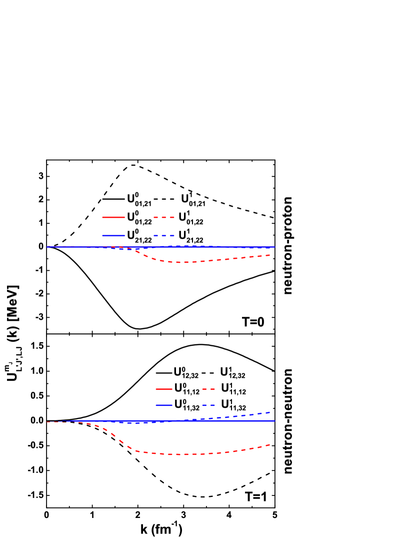
Figure 1: Nuclear potential as calculated from the off-diagonal matrix elements of $G$ matrix with the angular dependence of the propagator $Q/e(\omega)$. The upper (lower) panel corresponds to the neutron-proton (neutron-neutron) in the isospin singlet (triplet) state.

Compared to the AA, two primary changes stem from the angular dependence of the operator $Q/e(\omega)$. First, the off-diagonal matrix elements of $G$ matrix in $J$, i.e., $\langle J^{\prime}|G|J\rangle\neq 0$ [here the other variables are omitted] represent the coupling of different channels with fixed spin and isospin. These off-diagonal $G$ matrix elements result in a non vanishing contribution to the s.p. potentials. In the upper panel of Fig. 1 we show $U_{\ell^{\prime}J^{\prime},\ell J}^{m_{J}}(k)$ [which is obtained calculating Eq. (16) without the $TS\ell Jm_{j}$ summations] for the isospin-singlet neutron-proton scattering for symmetric nuclear matter at the empirical saturation density $\rho_{0}=0.17\text{fm}^{-3}$. In this figure, three kinds couplings, i.e., ($\ell^{\prime}=0,J^{\prime}=1;\ell=2,J=1$), ($\ell^{\prime}=0,J^{\prime}=1;\ell=2,J=2$) and ($\ell^{\prime}=2,J^{\prime}=1;\ell=2,J=2$), with $m_{J}=0,1$ are displayed. The sizable coupling ($\ell^{\prime}=0,J^{\prime}=1;\ell=2,J=1$) actually corresponds to the tensor force in the ${}^{3}SD_{1}$ channel which contains three $m_{j}$ components. For spin-up, i.e, $\sigma_{1}=\frac{1}{2}$, the Clebsch-Gordan coefficients and the properties of the spherical harmonics imply that the $m_{j}=-1$ components $U_{01,21}^{-1}(k)\equiv 0$. In addition, the Clebsch-Gordan coefficients and the properties of the spherical harmonics in Eq. (16) render the opposite values for the two components $U_{01,21}^{0}(k)$ and $U_{01,21}^{1}(k)$. However, they do not cancel each other completely since the $G$ matrix is nondegenerate for different $m_{j}$'s, that is, essentially originated from the angular dependence of the operators. This is the second major change when the AA approximation is not adopted. Due to the symmetries of $G$ matrix $\langle\ell^{\prime}J^{\prime}|G|\ell J\rangle_{-m_{J}}=(-)^{\ell^{\prime}-J^{\prime}+\ell-J}\langle\ell^{\prime}J^{\prime}|G|\ell J\rangle_{m_{J}}$, $U_{01,22}^{0}(k)$ and $U_{21,22}^{0}(k)$ are both equal to 0. The significant potential $U_{01,22}^{1}(k)$ corresponding to the coupling between ${}^{3}S_{1}$ and ${}^{3}D_{2}$ partial waves indicates that certain couplings, unexpected in the AA approximation, might contribute to some extent to the s.p. potential. For neutron-neutron, except the specific values, they are similar to the neutron-proton case shown in the lower panel of Fig.1.

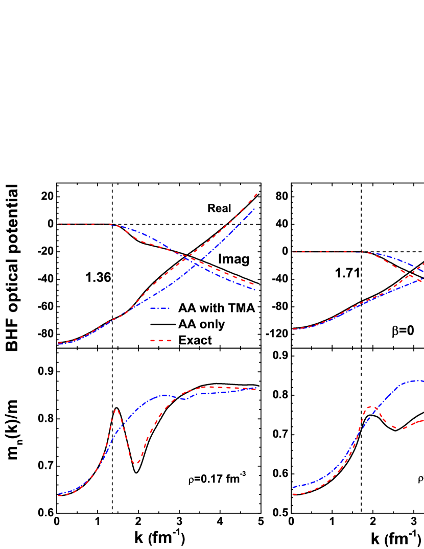
Figure 2: BHF optical potential and neutron effective-mass $m_{n}^{*}/m$ as a function of the momentum $k$ for symmetric nuclear matter at two densities with the exact calculation, the AA approximation, and the AA approximation with TMA, respectively.

To investigate the changes in the s.p. potential due to the angular dependence of the propagator, we report in the upper panels of Fig. 2 the BHF optical potential of symmetric nuclear matter in two cases with (solid line) and without (dashed line) the AA approximation for two typical densities $\rho_{0}$ and $2\rho_{0}$ , respectively. [Here,the BHF optical potential represent the on-shell value of Eq. (4).] Moreover, the results with the AA approximation including TMA, widely used in the previous works tbf2 ; tma1 ; tma2 ; tma3 ; tma4 ; tma5 , are reported as well. In calculating the BHF optical potential, one can actually employ Eq. (16) by considering the imaginary part of $G$ matrix as well as the real part, and $\textrm{Im}G$ corresponds to the imaginary part of the BHF optical potential. In the lower panels, the neutron effective mass vs. momentum , which are related to the derivative of the s.p. potential by $\frac{m_{\tau}^{*}}{m}(k)=\frac{k}{m}[\frac{d\varepsilon^{\tau}(k)}{dk}]^{-1}$, is also plotted. At the empirical saturation density $\rho_{0}$, compared to the exact scheme, the deviation resulting from the AA approximation is tiny for both potential and effective mass. This deviation grows up when increasing density, since the Pauli blocking effects become stronger and stronger. The procedure of handling with the $Q/e(\omega)$ becomes more important due to enhancing the Pauli blocking effect. When the TMA is also adopted, the potential deviation from the exact results is quite evident, especially for large momenta. Fortunately, the deviation is still tolerable below the Fermi momentum. The same as with the AA approximation, the deviation becomes more distinct at larger densities, due to the enhancement of the Pauli blocking. The effective mass in the AA approximation and TMA manifest a diversity similar to what happens with the potential. However, the difference looks more remarkable for the effective mass.

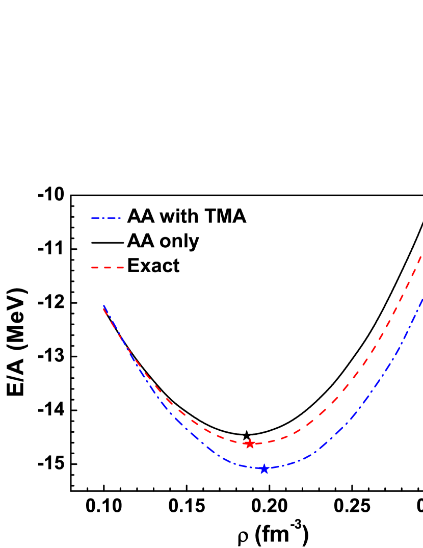
Figure 3: Equation of state (EOS) of symmetric nuclear matter with the exact calculation, the AA approximation, and the AA approximation with TMA, respectively. The star marks the saturation point in the three calculations.

In Fig. 3. we show the effects of the AA and TMA approximations on the EOS for symmetric nuclear matter. The saturation point ($\rho_{s}=0.197\text{fm}^{-3},E/A=-15.09\text{MeV}$) in the AA approximation with TMA coincides with that of Ref. tbf2 . The exact treatment of the total momentum substantially improves the saturation point. The saturation point within the AA approximation is about ($\rho_{s}=0.186\text{fm}^{-3},E/A=-14.47\text{MeV}$) approaching that of the exact calculation, $\rho_{s}=0.188\text{fm}^{-3},E/A=-14.62\text{MeV}$. As expected, AA approximation only leads to a small deviation of the EOS from the exact one. Although the discrepancy between the EOS of the exact calculation and the AA approximation plus TMA remains substantial.

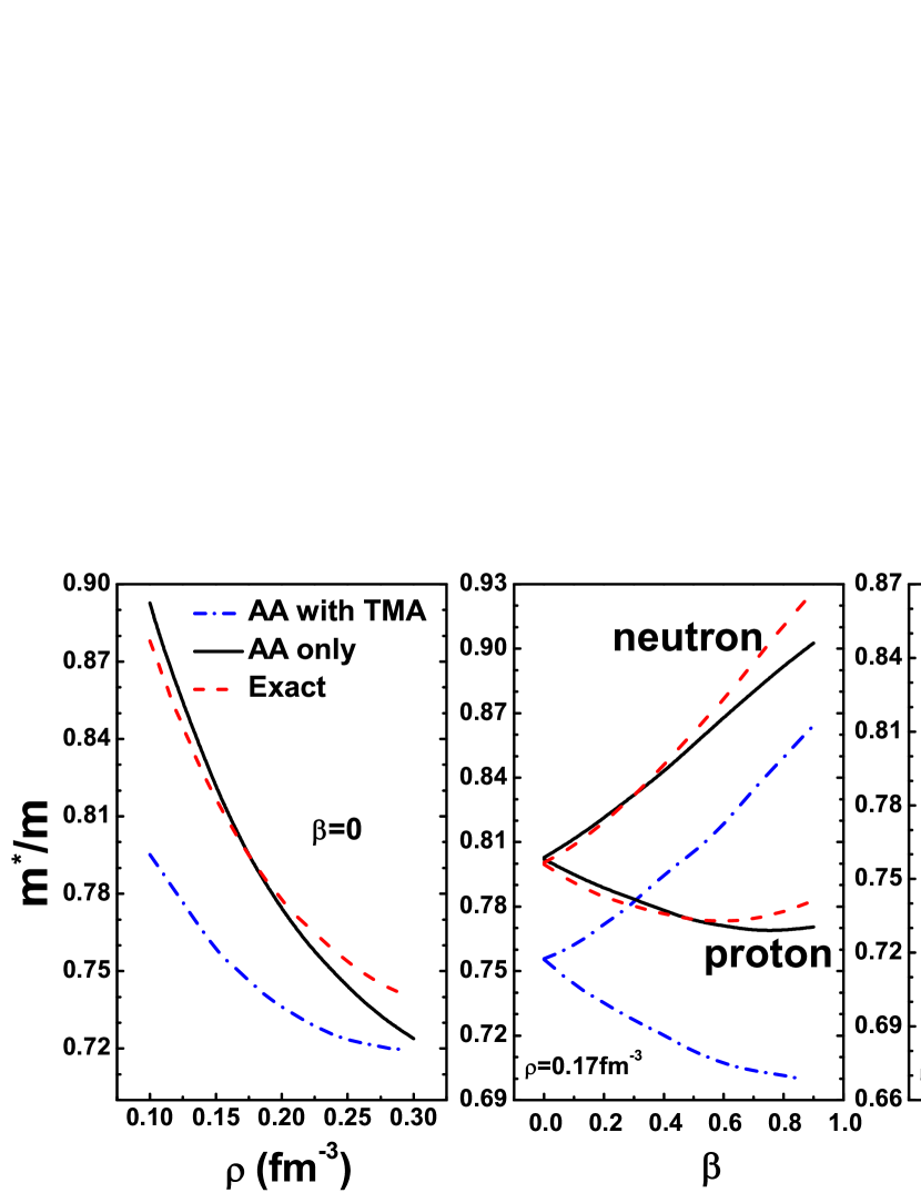
Figure 4: (Color online). Nucleon effective mass as a function of the density $\rho$ and the isospin asymmetry $\beta$ within the exact calculation, the AA approximation, and the AA approximation with TMA, respectively.

The nucleon effective mass is an important microscopic input to many studies of nuclear phenomena, such as the dynamics of heavy ion collisions at intermediate and high energies em1 , the damping of nuclear excitations and giant resonances em2 , and the thermal properties of neutron stars em3 ; em4 ; em5 ; em6 . Very important is the value of the effective mass at the Fermi surface, i.e., $m^{*}(k_{F})$ [hereafter the effective mass is referred to as $m^{*}(k_{F})$]. The density and isospin-asymmetry dependence of the effective mass is reported in Fig. 4 where the asymmetry parameter is defined as $\beta=(\rho_{n}-\rho_{p})/(\rho_{n}+\rho_{p})$ with the neutron (proton) density $\rho_{n}$ ($\rho_{p}$). The results in the AA approximation with TMA is consistent with that of Ref. mr1 . Above all, the effective-mass calculation with AA agrees well with the exact one at low density, but the discrepancy between the two grows with increasing density, being the enhancement attributed to the Pauli blocking effect. Similar to the potential, the difference between the exact and the AA approximation plus TMA seems noteworthy, although the difference tends to diminish at increasing densities. However, one should note that the proton effective mass decreases monotonically with the isospin asymmetry when the TMA is adopted. The proton effective mass in the exact calculation and AA exhibits a parabolic dependence on the isospin asymmetry.

IV SUMMARY

The equation of state of nuclear matter plays an important role in modern nuclear physics and astrophysics. The Brueckner-Bethe-Goldstone theory allows an ab initio calculation from microscopic potential. In the present investigation, an exact numerical treatment of the BG equation is performed to assess the reliability of the angular-average procedure of the operators $Q/e(\omega)$ as well as the total momentum approximation. In the exact treatment of the Pauli propagator, the previous definition of $Q/e(\omega)$ Eq.(3), which was adopted for symmetric nuclear matter, is proved to be inappropriate for asymmetric nuclear matter since it may lead to a mixing of the total isospin T=1 and T=0 neutron-proton states in $G$-matrix. Instead, we propose to symmetrize the Pauli propagator, i.e., Eq. (13), in our calculation to extend the definition of $Q/e$ for asymmetric matter, consistently with the symmetry $G(\beta)=G(-\beta)$. Accordingly we compare the s.p. potential, nucleon effective mass, and EOS in the three calculations with a microscopic 3BF, i.e., the exact calculation, the AA approximation, and the AA approximation plus TMA.

The calculations show that the exact treatment of the Pauli propagator results in inappreciable changes in the potential, effective mass, and binding energy at low densities. These changes grow slightly with density due to the enhancement of Pauli blocking. However, the AA procedure provides a fairly accurate simplifying approximation even when 3BF is applied. Instead, the total momentum of the intermediate two nucleons leads to a considerable contribution in predicting the saturation properties, the s.p. potential, and nucleon effective mass. And its replacement TMA is insufficient for accurate investigations of nuclear matter.

Appendix A Appendix

Let us consider, in fact, neutron-proton or proton-neutron matrix elements with $T_{z}=0$ in Eq. (8). When $T=0$, the summation over ${\tau_{1}\tau_{2}}$ reads

$$\sum_{\tau_{1}\neq\tau_{2}}(\frac{1}{2}\tau_{1}\frac{1}{2}\tau_{2}|T^{\prime}T_{z})(\frac{1}{2}\tau_{1}\frac{1}{2}\tau_{2}|TT_{z})F^{\tau_{1}\tau_{2}}(K,k,\hat{\emph{{k}}})\big{|}_{T^{\prime}=0}$$

$$= (\frac{1}{2}\frac{1}{2}\frac{1}{2}\frac{-1}{2}|00)(\frac{1}{2}\frac{1}{2}\frac{1}{2}\frac{-1}{2}|00)F^{pn}(K,k,\hat{\emph{{k}}})|_{T^{\prime}=0}$$

$$+ (\frac{1}{2}\frac{-1}{2}\frac{1}{2}\frac{1}{2}|00)(\frac{1}{2}\frac{-1}{2}\frac{1}{2}\frac{1}{2}|00)F^{np}(K,k,\hat{\emph{{k}}})|_{T^{\prime}=0}$$

$$= \frac{1}{2}[F^{pn}(K,k,\hat{\emph{{k}}})+F^{np}(K,k,\hat{\emph{{k}}})]|_{T^{\prime}=0}$$

$$= F^{pn}_{S}(K,k,\hat{\emph{{k}}})|_{T^{\prime}=0},$$

$$\sum_{\tau_{1}\neq\tau_{2}}(\frac{1}{2}\tau_{1}\frac{1}{2}\tau_{2}|T^{\prime}T_{z})(\frac{1}{2}\tau_{1}\frac{1}{2}\tau_{2}|TT_{z})F^{\tau_{1}\tau_{2}}(K,k,\hat{\emph{{k}}})\big{|}_{T^{\prime}=1}$$ (23)

$$= (\frac{1}{2}\frac{1}{2}\frac{1}{2}\frac{-1}{2}|10)(\frac{1}{2}\frac{1}{2}\frac{1}{2}\frac{-1}{2}|00)F^{pn}(K,k,\hat{\emph{{k}}})|_{T^{\prime}=1}$$

$$+ (\frac{1}{2}\frac{-1}{2}\frac{1}{2}\frac{1}{2}|10)(\frac{1}{2}\frac{-1}{2}\frac{1}{2}\frac{1}{2}|00)F^{np}(K,k,\hat{\emph{{k}}})|_{T^{\prime}=1}$$

$$= \frac{1}{2}[F^{pn}(K,k,\hat{\emph{{k}}})-F^{np}(K,k,\hat{\emph{{k}}})]|_{T^{\prime}=1}$$

$$= F^{pn}_{A}(K,k,\hat{\emph{{k}}})|_{T^{\prime}=1},$$

with the symmetric and antisymmetric parts of $F^{\tau_{1}\tau_{2}}$,

$$F^{pn}_{S}(K,k,\hat{\emph{{k}}})=\frac{1}{2}[F^{pn}(K,k,\hat{\emph{{k}}})+F^{pn}(K,k,-\hat{\emph{{k}}})]$$

$$F^{pn}_{A}(K,k,\hat{\emph{{k}}})=\frac{1}{2}[F^{pn}(K,k,\hat{\emph{{k}}})-F^{pn}(K,k,-\hat{\emph{{k}}})].$$ (24)

In deriving Eq. (A1), the properties of $F^{\tau_{1}\tau_{2}}$,

$$F^{\tau_{1}\tau_{2}}(K,k,\hat{\emph{{k}}})=F^{\tau_{2}\tau_{1}}(K,k,-\hat{\emph{{k}}})$$ (25)

should be adopted. For the case of $T=1$ and $T_{z}=0$ with the same procedure we get

$$\sum_{\tau_{1}\neq\tau_{2}}(\frac{1}{2}\tau_{1}\frac{1}{2}\tau_{2}|T^{\prime}T_{z})(\frac{1}{2}\tau_{1}\frac{1}{2}\tau_{2}|TT_{z})F^{\tau_{1}\tau_{2}}(K,k,\hat{\emph{{k}}})\big{|}_{T^{\prime}=1}$$

$$= F^{pn}_{S}(K,k,\hat{\emph{{k}}})|_{T^{\prime}=1}$$

$$\sum_{\tau_{1}\neq\tau_{2}}(\frac{1}{2}\tau_{1}\frac{1}{2}\tau_{2}|T^{\prime}T_{z})(\frac{1}{2}\tau_{1}\frac{1}{2}\tau_{2}|TT_{z})F^{\tau_{1}\tau_{2}}(K,k,\hat{\emph{{k}}})\big{|}_{T^{\prime}=0}$$ (26)

$$= F^{pn}_{A}(K,k,\hat{\emph{{k}}})|_{T^{\prime}=0}.$$

Equations (A1) and (A4) indicate that

$$\sum_{\tau_{1}\tau_{2}}(\frac{1}{2}\tau_{1}\frac{1}{2}\tau_{2}|T^{\prime}T_{z})(\frac{1}{2}\tau_{1}\frac{1}{2}\tau_{2}|TT_{z})F^{\tau_{1}\tau_{2}}(K,k,\hat{\emph{{k}}})$$ (27)

$$= F^{\tau_{1}\tau_{2}}_{S}(K,k,\hat{\emph{{k}}})|_{\delta_{TT^{\prime}}}+F^{\tau_{1}\tau_{2}}_{A}(K,k,\hat{\emph{{k}}})|_{\epsilon_{TT^{\prime}}}$$

for the case of $T_{z}=0$, where $\epsilon_{TT^{\prime}}=1-\delta_{TT^{\prime}}$. Once the proton-proton (neutron-neutron) matrix element with $T_{z}=1(-1)$ is calculated, Eq. (A5) is true as well with $F^{\tau_{1}\tau_{1}}_{A}\equiv 0$.

The property of $F^{\tau_{1}\tau_{2}}_{S}(K,k,\hat{\emph{{k}}})=F^{\tau_{1}\tau_{2}}_{S}(K,k,-\hat{\emph{{k}}})$ together with the well-known properties of the spherical harmonics, implies the identities,

$$\int d\hat{\emph{{k}}}Y^{*}_{\ell^{\prime}m_{\ell}^{\prime}}(\hat{\emph{{k}}})F^{\tau_{1}\tau_{2}}_{S}(K,k,\hat{\emph{{k}}})Y_{\ell m_{\ell}}(\hat{\emph{{k}}})$$

$$= \int d\hat{\emph{{k}}}Y^{*}_{\ell^{\prime}m_{\ell}^{\prime}}(-\hat{\emph{{k}}})F^{\tau_{1}\tau_{2}}_{S}(K,k,-\hat{\emph{{k}}})Y_{\ell m_{\ell}}(-\hat{\emph{{k}}})$$

$$= (-1)^{\ell^{\prime}+\ell}\int d\hat{\emph{{k}}}Y^{*}_{\ell^{\prime}m_{\ell}^{\prime}}(\hat{\emph{{k}}})F^{\tau_{1}\tau_{2}}_{S}(K,k,\hat{\emph{{k}}})Y_{\ell m_{\ell}}(\hat{\emph{{k}}}),$$

which conserves the parity. On the contrary, the term,

$$\int d\hat{\emph{{k}}}Y^{*}_{\ell^{\prime}m_{\ell}^{\prime}}(\hat{\emph{{k}}})F^{\tau_{1}\tau_{2}}_{A}(K,k,\hat{\emph{{k}}})Y_{\ell m_{\ell}}(\hat{\emph{{k}}})$$

$$= \int d\hat{\emph{{k}}}Y^{*}_{\ell^{\prime}m_{\ell}^{\prime}}(-\hat{\emph{{k}}})F^{\tau_{1}\tau_{2}}_{A}(K,k,-\hat{\emph{{k}}})Y_{\ell m_{\ell}}(-\hat{\emph{{k}}})$$

$$= -(-1)^{\ell^{\prime}+\ell}\int d\hat{\emph{{k}}}Y^{*}_{\ell^{\prime}m_{\ell}^{\prime}}(\hat{\emph{{k}}})F^{\tau_{1}\tau_{2}}_{A}(K,k,\hat{\emph{{k}}})Y_{\ell m_{\ell}}(\hat{\emph{{k}}}),$$

violates the parity conservation. Fortunately, with the help of $\epsilon_{TT^{\prime}}$ and $\delta_{SS^{\prime}}$ one can demonstrate that this term maintains the generalized Pauli principle selection rule $(-1)^{T+S+\ell}=-1$.

References

• (1) K. Hebeler, S. K. Bogner, R. J. Furnstahl, A. Nogga, and A. Schwenk, Phys. Rev. C 83, 031301(R) (2011).
• (2) I. Tews, T. Kr$\ddot{u}$ger, K. Hebeler, and A. Schwenk, Phys. Rev. Lett. 110, 032504 (2013).
• (3) J.W. Holt, N. Kaiser, and W. Weise, Prog. Part. Nucl. Phys. 73, 35 (2013).
• (4) C. Wellenhofer, J.W. Holt, and N. Kaiser, Phys. Rev. C 92, 015801 (2015).
• (5) C. Drischler, K. Hebeler, and A. Schwenk, Phys. Rev. Lett. 122, 042501 (2019).
• (6) V. R. Pandharipande and R. B. Wiringa, Rev. Mod. Phys. 51, 821 (1979).
• (7) F. Arias de Saavedra, C. Bisconti, G. Co , and A. Fabrocini, Phys. Rep. 450, 1 (2007).
• (8) B. S. Pudliner, V. R. Pandharipande, J. Carlson, and R. B. Wiringa, Phys. Rev. Lett. 74, 4396 (1995).
• (9) K. E. Schmidt and S. Fantoni, Phys. Lett. B 446, 99 (1999).
• (10) S. C. Pieper and R. B. Wiringa, Annu. Rev. Nucl. Part. Sci. 51, 53 (2001).
• (11) J. Carlson, J. Morales Jr., V. R. Pandharipande, and D. G. Ravenhall, Phys. Rev. C 68, 025802 (2003).
• (12) A. Gezerlis and J. Carlson, Phys. Rev. C 81, 025803 (2010).
• (13) G. Wlazlowski and P. Magierski, Phys. Rev. C 83, 012801 (2011).
• (14) B.D. Day, Rev. Mod. Phys. 39, 719 (1967).
• (15) M. Baldo, I. Bombaci, G. Giansiracusa, U. Lombardo, C. Mahaux, and R. Sartor, Phys. Rev. C 41 1748 (1990); Nucl. Phys. A 545 741 (1992).
• (16) A. Ramos, A. Polls, and W. Dickoff, Nucl. Phys. A 551, 45 (1993).
• (17) T. Alm et al., Nucl. Phys. A 551, 45 (1993).
• (18) A. Rios, A. Polls, A. Ramos, and H. Muther, Phys. Rev. C 74, 054317 (2006).
• (19) A. Rios, A. Polls, and I.Vidana, Phys. Rev. C 79, 025802 (2009).
• (20) K.A. Brueckner, J.L. Gammel, Phys. Rev. 109, 1023 (1958).
• (21) M. I. Haftel, F. Tabakin, Nucl. Phys. A 158, 1 (1970).
• (22) T. Cheon and E. F. Redish, Phys. Rev. C 39, 331 (1989).
• (23) E. Schiller, H. M uther, and P. Czerski, Phys. Rev. C 59, 2934 (1999); 60, 059901(E) (1999).
• (24) K. Suzuki, R. Okamoto, M. Kohno, and S. Nagata, Nucl. Phys. A 665, 92 (2000).
• (25) F. Sammarruca, X. Meng, and E. J. Stephenson, Phys. Rev. C 62, 014614 (2000).
• (26) E. J. Stephenson, R. C. Johnson, and F. Sammarruca, Phys. Rev. C 71, 014612 (2005).
• (27) T. Frick, Kh. Gad, H. M uther, and P. Czerski, Phys. Rev. C 65, 034321 (2002).
• (28) R. Sartor, Phys. Rev. C 54, 809 (1996).
• (29) H. F. Arellano, and J.-P. Delaroche, Phys. Rev. C 83, 044306 (2011).
• (30) R. V. Reid, Ann. Phys. (N.Y.) 50, 411 (1968).
• (31) P. Grangé, A. Lejeune, M. Martzolff, and J.-F. Mathiot, Phys. Rev. C 40, 1040 (1989).
• (32) W. Zuo, A. Lejeune, U. Lombardo, and J.-F. Mathiot, Nucl. Phys. A 706, 418 (2002); Eur. Phys. J. A 14, 469 (2002).
• (33) K. A. Brueckner, S. A. Coon, and J. Dabrowski, Phys. Rev. 168, 1184 (1968).
• (34) I. Bombaci and U. Lombardo, Phys. Rev. C 44, 1892 (1991).
• (35) W. Zuo, I. Bombaci, and U. Lombardo, Phys. Rev. C 60, 024605 (1999).
• (36) I. Bombaci, T. T. S. Kuo, and U. Lombardo, Phys. Rep. 242, 165 (1994).
• (37) W. Zuo, Z. H. Li, A. Li, and G. C. Lu, Phys. Rev. C 69, 064001 (2004).
• (38) S. S. Zhang, L. G. Cao, U. Lombardo and P. Schuck, Phys. Rev. C 93 044329 (2016).
• (39) P. Wang and W. Zuo, Chin. Phys. C 39 014101 (2015).
• (40) P. Yin, J.-M. Dong, and W. Zuo, Chin. Phys. C 41 114102 (2017).
• (41) D. Alonso and F. Sammarruca, Phys. Rev. C 67, 054301 (2003).
• (42) F. Sammarruca, B. Chen, L. Coraggio, N. Itaco, and R. Machleidt, Phys. Rev. C 86, 054317 (2012).
• (43) F. Sammarruca, Eur. Phys. J. A 50, 22 (2014).
• (44) H. Tong, X.-L. Ren, P. Ring, S.-H. Shen, S.-B. Wang, and J. Meng, Phys. Rev. C 98, 054302 (2018).
• (45) W. Zuo, I. Bombaci, and U. Lombardo, Phys. Rev. C 60 024605 (1999).
• (46) N. Kaiser, Eur. Phys. J. A 48, 58 (2012).
• (47) A. Dyhdalo, R. J. Furnstahl, K. Hebeler, and I. Tews, Phys. Rev. C 94, 034001 (2016).
• (48) J. Cugnon, A. Lejeune, and P. Grang e, Phys. Rev. C 35, R861 (1987).
• (49) G. F. Bertsch, P. F. Bortignon, and R. A. Broglia, Rev. Mod. Phys. 55, 287 (1983).
• (50) D. Page, J. M. Lattimer, M. Prakash, and A. W. Steiner, ApJS 155, 623 (2004).
• (51) M. Baldo and G. F. Burgio, Rep. Prog. Phys. 75, 026301 (2012).
• (52) X. L. Shang, A. Li, Z. Q. Miao, G. F. Burgio, and H.-J. Schulze, Phys. Rev. C 101 065801 (2020).
• (53) P. Yin, X.-H. Fan, J.-M. Dong, W.-M. Guo and W. Zuo, Nucl. Phys. A 961, 200 (2017).
• (54) W. Zuo, U. Lombardo, H.-J. Schulze, and Z. H. Li, Phys. Rev. C 74 014317 (2006).