Local2Global: Scaling global representation learning on graphs via local training

Abstract.

We propose a decentralised “local2global” approach to graph representation learning, that one can a-priori use to scale any embedding technique. Our local2global approach proceeds by first dividing the input graph into overlapping subgraphs (or “patches”) and training local representations for each patch independently. In a second step, we combine the local representations into a globally consistent representation by estimating the set of rigid motions that best align the local representations using information from the patch overlaps, via group synchronization. A key distinguishing feature of local2global relative to existing work is that patches are trained independently without the need for the often costly parameter synchronisation during distributed training. This allows local2global to scale to large-scale industrial applications, where the input graph may not even fit into memory and may be stored in a distributed manner. Preliminary results on medium-scale data sets (up to $\sim$7K nodes and $\sim$200K edges) are promising, with a graph reconstruction performance for local2global that is comparable to that of globally trained embeddings. A thorough evaluation of local2global on large scale data and applications to downstream tasks, such as node classification and link prediction, constitutes ongoing work.

1. Introduction

The application of deep learning on graphs, or Graph Neural Networks (GNNs), has recently gained considerable attention. Among the significant open challenges in this area of research is the question of scalability. Cornerstone techniques such as Graph Convolutional Networks (GCNs) (Kipf and Welling, 2017) make the training dependent on the neighborhood of any given node. Since in many real-world graphs the number of neighbors grows exponentially with the number of hops taken, the scalability of such methods is a significant challenge. In recent years, several techniques have been proposed to make GCNs more scalable, including layer-wise sampling (Hamilton et al., 2018) and subgraph sampling (Chiang et al., 2019) approaches (see section 2).

We contribute to this line of work by proposing a decentralised divide-and-conquer approach to improve the scalability of network embedding techniques. Our “local2global” approach proceeds by first dividing the network into overlapping subgraphs (or “patches”) and training separate local node embeddings for each patch (local in the sense that each patch is embedded into its own local coordinate system). The resulting local patch node embeddings are then transformed into a global node embedding (i.e. all nodes embedded into a single global coordinate system) by estimating a rigid motion applied to each patch using the As-Synchronized-As-Possible (ASAP) algorithm (Cucuringu et al., 2012b, a). A key distinguishing feature of this “decentralised” approach is that we can train the different patch embeddings separately, without the need to keep parameters synchronised. The benefit of local2global is threefold: (1) it is highly parallelisable as each patch is trained independently; (2) it can be used in privacy-preserving applications and federated learning setups, where frequent communication between devices is often a limiting factor (Kairouz and McMahan, 2021), or “decentralized” organizations, where one needs to simultaneously consider data sets from different departments; (3) it can reflect varying structure across a graph through asynchronous parameter learning. Another important advantage of our local2global approach is that it can be directly applied to improve the scalability of a large variety of network embedding techniques (Goyal and Ferrara, 2018), unlike most of the existing approaches reviewed in section 2 which are restricted to GCNs.

2. Related work

The key scalability problems for GCNs only concern deep architectures where we have $l$ nested GCN layers. In particular, a single-layer GCN is easy to train in a scalable manner using mini-batch stochastic gradient descent (SGD). For simplicity, assume that we have a fixed feature dimension $d$, i.e., $d_{\text{in}}=d_{\text{out}}=d$ for all layers. The original GCN paper (Kipf and Welling, 2017) uses full-batch gradient descent to train the model which entails the computation of the gradient for all nodes before updating the model parameters. This is efficient in terms of time complexity per epoch ($O(lmd+lnd^{2})$) where $n$ is the number of nodes and $m$ is the number of edges. However, it requires storing all the intermediate embeddings and thus has memory complexity $O(lnd+ld^{2})$. Further, as there is only a single parameter update per epoch, convergence tends to be slow.

The problem with applying vanilla mini-batch SGD (where we only compute the gradient for a sample of nodes, i.e., the batch) to a deep GCN model is that the embedding of the nodes in the final layer depends on the embedding of all the neighbours of the nodes in the previous layer and so on iteratively. Therefore the time complexity for a single mini-batch update approaches that for a full-batch update as the number of layers increases, unless the network has disconnected components. There are mainly three families of methods (Chen et al., 2020; Chiang et al., 2019) that have been proposed to make mini-batch SGD training more efficient for GCNs.

Layer-wise sampling.:

The idea behind layer-wise sampling is to sample a set of nodes for each layer of the nested GCN model and compute the embedding for sampled nodes in a given layer only based on embeddings of sampled nodes in the previous layer rather than considering all the neighbours as would be the case for vanilla SGD. This seems to have first been used by GraphSAGE (Hamilton et al., 2018), where a fixed number of neighbours is sampled for each node at each layer. However, this results in a computational complexity that is exponential in the number of layers and also redundant computations as the same intermediate nodes may be sampled starting from different nodes in the batch. Later methods avoid the exponential complexity by first sampling a fixed number of nodes for each layer either independently (FastGCN (Chen et al., 2018a)) or conditional on being connected to sampled nodes in the previous layer (LADIES (Zou et al., 2019)) and reusing embeddings. Both methods use importance sampling to correct for bias introduced by non-uniform node-sampling distributions. Also notable is (Chen et al., 2018b), which uses variance reduction techniques to effectively train a GCN model using neighbourhood sampling as in GraphSAGE with only 2 neighbours per node. However, this is achieved by storing hidden embeddings for all nodes in all layers and thus has the same memory complexity as full-batch training.

Linear model.:

Linear models remove the non-linearities between the different GCN layers which means that the model can be expressed as a single-layer GCN with a more complicated convolution operator and hence trained efficiently using mini-batch SGD. Common choices for the convolution operator are powers of the normalised adjacency matrix (Wu et al., 2019) and variants of personalised Page-Rank (PPR) matrices (Busch et al., 2020; Chen et al., 2020; Bojchevski et al., 2020; Klicpera et al., 2019). Another variant of this approach is (Frasca et al., 2020), which proposes combining different convolution operators in a wide rather than deep architecture. There are different variants of the linear model architecture, depending on whether the non-linear feature transformation is applied before or after the propagation (see (Busch et al., 2020) for a discussion), leading to predict-propagate and propagate-predict architectures respectively. The advantage of the propagate-predict architecture is that one can pre-compute the propagated node features (e.g., using an efficient push-based algorithm (Chen et al., 2020)) which can make training highly scalable. The disadvantage is that this will densify sparse features which can make training harder (Bojchevski et al., 2020). However, the results from (Busch et al., 2020) suggest that there is usually not much difference in prediction performance between these options (or the combined architecture where trainable transformations are applied before and after propagation).

Subgraph sampling.:

Subgraph sampling techniques (Zeng et al., 2019; Chiang et al., 2019; Zeng et al., 2020) construct batches by sampling an induced subgraph of the full graph. In particular, for subgraph sampling methods, the sampled nodes in each layer of the model in a batch are the same. In practice, subgraph sampling seems to outperform layer-wise sampling (Chen et al., 2020). GraphSAINT (Zeng et al., 2020), which uses a random-walk sampler with an importance sampling correction similar to (Chen et al., 2018a; Zou et al., 2019), seems to have the best performance so far. Our local2global approach shares similarities with subgraph sampling, most notably ClusterGCN (Chiang et al., 2019), which uses graph clustering techniques to sample the batches. The key distinguishing feature of our approach is that we train independent models for each patch whereas for ClusterGCN, model parameters have to be kept in sync for different batches, which hinders fully distributed training and its associated key benefits (see section 1).

3. LOCAL2GLOBAL algorithm

The key idea behind the local2global approach to graph embedding is to embed different parts of a graph independently by splitting the graph into overlapping “patches” and then stitching the patch node embeddings together to obtain a global node embedding. The stitching of the patch node embeddings proceeds by estimating the rotations/reflections and translations for the embedding patches that best aligns them based on the overlapping nodes.

Consider a graph $G(V,E)$ with node set $V$ and edge set $E$. The input for the local2global algorithm is a patch graph $G_{p}(\mathcal{P},E_{p})$, where each node (i.e., a “patch”) of the patch graph is a subset of $V$ and each patch $P_{k}\in\mathcal{P}$ is associated with an embedding $\bm{X}^{(k)}\in\mathbb{R}^{|P_{k}|\times d}$. We require that the set of patches $\mathcal{P}=\{P_{k}\}_{k=1}^{p}$ is a cover of the node set $V$ (i.e., $\bigcup_{k=1}^{p}P_{k}=V$), and that the patch embeddings all have the same dimension $d$. We further assume that the patch graph is connected and that the patch edges satisfy the minimum overlap condition $\{P_{i},P_{j}\}\in E_{p}\implies|P_{i}\cap P_{j}|\geq d+1$. Note that a pair of patches that satisfies the minimum overlap condition is not necessarily connected in the patch graph.

The local2global algorithm for aligning the patch embeddings proceeds in two stages and is an evolution of the approach in (Cucuringu et al., 2012b, a). We assume that each patch embedding $\bm{X}^{(k)}$ is a perturbed part of an underlying global node embedding $\bm{X}$, where the perturbation is composed of reflection ($Z_{2}$), rotation (SO($d$)), translation ($\mathbb{R}^{d}$), and noise. The goal is to estimate the transformation applied to each patch using only pairwise noisy measurements of the relative transformation for pairs of connected patches. In the first stage, we estimate the orthogonal transformation to apply to each patch embedding, using a variant of the eigenvector synchronisation method (Singer, 2011; Cucuringu et al., 2012b, a). In the second stage, we estimate the patch translations by solving a least-squares problem. Note that unlike (Cucuringu et al., 2012b, a), we solve for translations at the patch level rather than solving a least squares problem for the node coordinates. This means that the computational cost for computing the patch alignment is independent of the size of the original network and depends only on the amount of patch overlap, the number of patches and the embedding dimension.

3.1. Eigenvector synchronisation over orthogonal transformations

We assume that to each patch $P_{i}$, there corresponds an unknown group element $S_{i}\in O(d)\simeq Z_{2}\times SO(d)$ (represented by a $d\times d$ orthogonal matrix), and for each pair of connected patches $(P_{i},P_{j})\in E_{p}$ we have a noisy proxy for $S_{i}S_{j}^{-1}$, which is precisely the setup of the group synchronization problem.

For a pair of connected patches $P_{i},P_{j}\in\mathcal{P}$ such that $\{P_{i},P_{j}\}\in E_{p}$ we can estimate the relative rotation/reflection by applying the method from (Horn et al., 1988) to their overlap as $|P_{i}\cap P_{j}|\geq d+1$. Thus, we can construct a block matrix $\bm{R}$ where $\bm{R}_{ij}$ is the $d\times d$ orthogonal matrix representing the estimated relative transformation from patch $P_{j}$ to patch $P_{i}$ if $\{P_{i},P_{j}\}\in E_{p}$ and $\bm{R}_{ij}=\bm{0}$ otherwise, such that $\bm{R}_{ij}\approx\bm{S}_{i}\bm{S}_{j}^{T}$ for connected patches.

In the noise-free case, we have the consistency equations $\bm{S}_{i}=\bm{R}_{ij}\bm{S}_{j}$ for all $i,j$ such that $\{P_{i},P_{j}\}\in E_{p}$. We can combine the consistency equations for all neighbours of a patch to get

(1) $$\bm{S}_{i}=\bm{M}_{ij}\bm{S}_{j},\qquad\bm{M}_{ij}=\frac{\sum_{j}w_{ij}\bm{R}_{ij}}{\sum_{j}w_{ij}},$$

where we use $w_{ij}=|P_{i}\cap P_{j}|$ to weight the contributions as we expect a larger overlap to give a more robust estimate of the relative transformation. We can write eq. 1 as $\bm{S}=\bm{M}\bm{S}$, where $\bm{S}=(\bm{S}_{1},\ldots,\bm{S}_{p})^{T}$ is a $pd\times d$ block-matrix and $\bm{M}$ is a $pd\times pd$ block-matrix. Thus, in the noise-free case, the columns of $\bm{S}$ are eigenvectors of $\bm{M}$ with eigenvalue 1. Thus, following (Cucuringu et al., 2012b, a), we can use the $d$ leading eigenvectors of $\bm{M}$ as the basis for estimating the transformations. Let $\bm{U}=(\bm{U}_{1},\ldots,\bm{U}_{p})^{T}$ be the $pd\times d$ matrix whose columns are the $d$ leading eigenvectors of $\bm{M}$, where $\bm{U}_{i}$ is the $d\times d$ block of $\bm{U}$ corresponding to patch $P_{i}$. We obtain the estimate $\hat{\bm{S}}_{i}$ of $\bm{S}_{i}$ by finding the nearest orthogonal transformation to $\bm{U}_{i}$ using an SVD (Horn et al., 1988), and hence the estimated rotation-synchronised embedding of patch $P_{i}$ is $\hat{\bm{X}}^{(i)}=\bm{X}^{(i)}\hat{\bm{S}}_{i}^{T}$.

3.2. Synchronisation over translations

After synchronising the rotation of the patches, we can estimate the translations by solving a least squares problem. Let $\hat{\bm{X}}_{i}^{(k)}\in\mathbb{R}^{d}$ be the (rotation-synchronised) embedding of node $i$ in patch $P_{k}$ ($\hat{\bm{X}}_{i}^{(k)}$ is only defined if $i\in P_{k}$). Let $\bm{T}_{k}\in\mathbb{R}^{d}$ be the translation of patch $k$, then in the noise-free case we have the consistency equations

(2) $$\hat{\bm{X}}_{i}^{(k)}+\bm{T}_{k}=\hat{\bm{X}}_{i}^{(l)}+\bm{T}_{l},\qquad i\in P_{k}\cap P_{l}.$$

We can combine the conditions in eq. 2 for each edge in the patch graph to obtain

(3) $$\bm{B}\bm{T}=\bm{C},\qquad\bm{C}_{(P_{k},P_{l})}=\frac{\sum_{i\in P_{k}\cap P_{l}}\hat{\bm{X}}_{i}^{(k)}-\hat{\bm{X}}_{i}^{(l)}}{|P_{k}\cap P_{l}|},$$

where $\bm{T}\in\mathbb{R}^{|\mathcal{P}|\times d}$ is the matrix such that the $k$th row of $\bm{T}$ is the translation $\bm{T}_{k}$ of patch $P_{k}$ and $\bm{B}\in\{-1,1\}^{|E_{p}|\times|\mathcal{P}|}$ is the incidence matrix of the patch graph with entries $\bm{B}_{(P_{k},P_{l}),j}=\delta_{lj}-\delta_{kj}$, where $\delta_{ij}$ denotes the Kronecker delta. Equation 3 defines an overdetermined linear system that has the true patch translations as a solution in the noise-free case. In the practical case of noisy patch embeddings, we can instead solve eq. 3 in the least-squares sense

(4) $$\hat{\bm{T}}=\operatorname*{arg\,min}_{\bm{T}\in\mathbb{R}^{p\times d}}\left\|\bm{B}\bm{T}-\bm{C}\right\|_{2}^{2}.$$

We estimate the aligned node embedding $\bar{\bm{X}}$ in a final step using the centroid of the aligned patch embeddings of a node, i.e.,

$$\bar{\bm{X}}_{i}=\frac{\sum_{\{P_{k}\in\mathcal{P}\colon i\in P_{k}\}}\hat{\bm{X}}_{i}^{(k)}+\hat{\bm{T}}_{k}}{|\{P_{k}\in\mathcal{P}\colon i\in P_{k}\}|}.$$

3.3. Scalability of the local2global algorithm

The patch alignment step of local2global is highly scalable and does not directly depend on the size of the input data. The cost for computing the matrix $M$ is $O(|E_{p}|od^{2})$ where $o$ is the average overlap between connected patches (typically $o\sim d$) and the cost for computing the vector $b$ is $O(|E_{p}|od)$. Both operations are trivially parallelisable over patch edges. The translation problem can be solved with an iterative least-squares solver with a per-iteration complexity of $O(|E_{p}|d)$. The limiting step for local2global is usually the synchronisation over orthogonal transformations which requires finding $d$ eigenvectors of a $d|\mathcal{P}|\times d|\mathcal{P}|$ sparse matrix with $|E_{p}|d^{2}$ non-zero entries for a per-iteration complexity of $O(|E_{p}|d^{3})$. This means that in the typical scenario where we want to keep the patch size constant, the patch alignment scales almost linearly with the number of nodes in the dataset, as we can ensure that the patch graph remains sparse, such that $|E_{p}|$ scales almost linearly with the number of patches. The $O(|E_{p}|d^{3})$ scaling puts some limitations on the embedding dimension attainable with the local2global approach, though, as we can see from the experiments in section 4.4, it remains feasible for reasonably high embedding dimension.

The preprocessing to divide the network into patches scales as $O(m)$. The speed-up attainable due to training patches in parallel depends on the oversampling ratio (i.e., the total number of edges in all patches divided by the number of edges in the original graph). As seen in section 4.4, we achieve good results with moderate oversampling ratios.

4. Experiments

4.1. Data sets

We consider two data sets to test the viability of the local2global approach to graph embeddings, the Cora citation data set from (Yang et al., 2016) and the Amazon photo data set from (Shchur et al., 2019). We consider only nodes and edges in the largest connected component (LCC). We show some statistics of the data sets in table 1.

	nodes in LCC	edges in LCC	features
Cora	$2485$	$10\,138$	$1433$
Amazon photo	$7487$	$238\,086$	$745$

Table 1. Data sets

Input: $G_{p}(\mathcal{P},E_{p})$, $G(V,E)$, target patch degree $k$

Result: sparsified patch graph $G_{p}(\mathcal{P},\tilde{E}_{p})$

foreach $\{P_{i},P_{j}\}\in E_{p}$ do

Compute conductance weight

    $$c_{ij}=\frac{|\{(u,v)\in E:u\in P_i,v\in P_j\}|}{\min (|\{(u,v)\in E:u\in P_i\}|,|\{(u,v)\in E:u\in P_j\}|)};$$

      

foreach $\{P_{i},P_{j}\}\in E_{p}$ do

       Compute effective resistance $r_{ij}$ between $P_{i}$ and $P_{j}$ in $G_{p}(\mathcal{P},E_{p},c)$ using the algorithm of (Spielman and Srivastava, 2011);

       Let $w_{ij}=r_{ij}c_{ij}$;

      

Initialize $\tilde{E}_{p}$ with a maximum spanning tree of $G_{p}(\mathcal{P},E_{p},w)$;

Sample the remaining $(k-1)p+1$ edges from $E_{p}\setminus\tilde{E}_{p}$ without replacement and add them to $\tilde{E}_{p}$, where edge $\{P_{i},P_{j}\}$ is sampled with probability $w_{ij}$;

return $G_{p}(\mathcal{P},\tilde{E}_{p})$

Algorithm 1 Sparsify patch graph

Input: $\mathcal{C}$, $E_{p}$, $G(V,E)$, min overlap $l$, max overlap $u$

Result: Overlapping patches $\mathcal{P}$

Initialise $\mathcal{P}=\mathcal{C}$;

Define the neighbourhood of a set of nodes $U$ as

$$N(U)=\{j:i\in U,(i,j)\in E,j\notin U\};$$

foreach $P_{i}\in\mathcal{P}$ do

       foreach $P_{j}$ s.t. $\{P_{i},P_{j}\}\in E_{p}$ do

             Let $F=N(C_{i})\cap C_{j}$;

             while $|P_{i}\cap C_{j}|<l/2$ do

                   if $|F|+|P_{i}\cap C_{j}|>u/2$ then

                         reduce $F$ by sampling uniformly at random such that $|F|=u/2-|P_{i}\cap C_{j}|$;

                  Let $P_{i}=P_{i}\cup F$;

                   Let $F=(N(F)\cap C_{j})\setminus P_{i}$;

                  

            

      

return $\mathcal{P}$

Algorithm 2 Create overlapping patches

4.2. Patch graph construction

The first step in the local2global embedding pipeline is to divide the network $G(V,E)$ into overlapping patches. In some federated-learning applications, the network may already be partitioned and some or all of the following steps may be skipped provided the resulting patch graph is connected and satisfies the minimum overlap condition for the desired embedding dimension. Otherwise, we proceed by first partitioning the network into non-overlapping clusters and then enlarging clusters to create overlapping patches. This two-step process makes it easier to ensure that patch overlaps satisfy the conditions for the local2global algorithm without introducing excessive overlaps than if we were to use a clustering algorithm that produces overlapping clusters directly. We use the following pipeline to create the patches:

• Partition the network into $p$ non-overlapping clusters $\mathcal{C}=\{C_{k}\}_{k=1}^{p}$ such that $|C_{k}|\geq\frac{d+1}{2}$ for all $k$. We use METIS (Karypis and Kumar, 1998) to cluster the networks for the experiments in section 4.4. However, for very large networks, more scalable clustering algorithms such as FENNEL (Tsourakakis et al., 2014) could be used.

• Initialize the patches to $\mathcal{P}=\mathcal{C}$ and define the patch graph $G_{p}(\mathcal{P},E_{p})$, where $\{P_{i},P_{j}\}\in E_{p}$ iff there exist nodes $i\in P_{i}$ and $j\in P_{j}$ such that $\{i,j\}\in E$. (Note that if $G$ is connected, $G_{p}$ is also connected.)

• Sparsify the patch graph $G_{p}$ to have mean degree $k$ using algorithm 1 adapted from the effective-resistance sampling algorithm of (Spielman and Srivastava, 2011).

• Expand the patches to create the desired patch overlaps. We define a lower bound $l\geq d+1$ and upper bound $u$ for the desired patch overlaps and use algorithm 2 to expand the patches such that $|P_{i}\cap P_{j}|\geq l$ for all $\{P_{i},P_{j}\}\in E_{p}$.

For Cora, we split the network into 10 patches and sparsify the patch graph to a target mean degree $k=4$. We set the lower bound for the overlap to $l=129$ and upper bound to $u=256$. For Amazon photo, we split the network into 20 patches and sparsify the patch graph to a target mean degree of $k=5$. We set the lower bound for the overlap to $l=256$ and the upper bound to $u=512$.

4.3. Embedding model

As embedding method we consider the variational graph auto-encoder (VGAE) architecture of (Kipf and Welling, 2016). We use the Adam optimizer (Kingma and Ba, 2015) for training with learning rate set to 0.01 for Cora and 0.001 for Amazon photo and train all models for 200 epochs. We set the hidden dimension of the models to $2\times d$ for Cora and to $4\times d$ for Amazon photo where $d$ is the embedding dimension.

4.4. Results

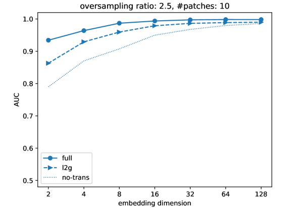
(a) Cora

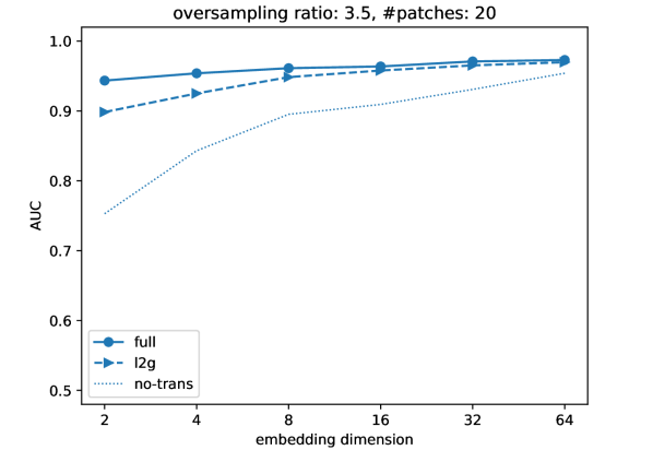
(b) Amazon photo

Figure 1. AUC network reconstruction score as function of embedding dimension using full data or stitched patch embeddings for 1 Cora and 1 Amazon photo.

As a first test case for the viability of the local2global approach, we consider a network reconstruction task. We train the models using all edges in the largest connected component and compare three training scenarios

full::

Model trained on the full data.

l2g::

Separate models trained on the subgraph induced by each patch and stitched using the local2global algorithm.

no-trans::

Same training as l2g but node embeddings are obtained by taking the centroid over patch embeddings that contain the node without applying the alignment transformations.

We evaluate the network reconstruction error using the AUC scores based on all edges in the largest connected component as positive examples and the same number of randomly sampled non-edges as negative examples. We train the models for 200 epochs using full-batch gradient descent. We show the results in fig. 1. For ‘full’, we report the best result out of 10 training runs. For ‘l2g’ and ‘no-trans’, we first identify the best model out of 10 training runs on each patch and report the results for stitching the best models.

Overall, the gap between the results for ‘l2g‘ and ‘full‘ is small and essentially vanishes for higher embedding dimensions. The aligned ‘l2g‘ embeddings consistently outperform the unaligned ‘no-trans’ baseline.

5. Conclusion

In this work, we introduced a framework that can significantly improve the computational scalability of generic graph embedding methods, rendering them scalable to real-world applications that involve massive graphs, potentially with millions or even billions of nodes. At the heart of our pipeline is the local2global algorithm, a divide-and-conquer approach that first decomposes the input graph into overlapping clusters (using one’s method of choice), computes entirely local embeddings via the preferred embedding method, for each resulting cluster (exclusively using information available at the nodes within the cluster), and finally stitches the resulting local embeddings into a globally consistent embedding, using established machinery from the group synchronization literature.

Our preliminary results on medium-scale data sets are promising and achieve comparable accuracy on graph reconstruction as globally trained VGAE embeddings. Our ongoing work consists of two keys steps. A first is to further demonstrate the scalability benefits of local2global on large-scale data sets using a variety of embedding techniques and downstream tasks by comparing with state-of-the-art synchronised subgraph sampling methods, as well as exploring the trade-off between parallelisability and embedding quality as a function of patch size and overlap. A second is to demonstrate particular benefits of locality and asynchronous parameter learning. These have clear advantages for privacy preserving and federated learning setups. It would also be particularly interesting to assess the extent to which this local2global approach can outperform global methods. The intuition and hope in this direction stems from the fact that asynchronous locality can be construed as a regularizer (much like sub-sampling, and similar to dropout) and could potentially lead to better generalization and alleviate the oversmoothing issues of deep GCNs, as observed in (Chiang et al., 2019).

References

- (1)
- Bojchevski et al. (2020) Aleksandar Bojchevski, Johannes Klicpera, Bryan Perozzi, Amol Kapoor, Martin Blais, Benedek Rózemberczki, Michal Lukasik, and Stephan Günnemann. 2020. Scaling Graph Neural Networks with Approximate PageRank. In Proceedings of the 26th ACM SIGKDD International Conference on Knowledge Discovery & Data Mining (KDD ’20). ACM, USA, 2464–2473.
- Busch et al. (2020) Julian Busch, Jiaxing Pi, and Thomas Seidl. 2020. PushNet: Efficient and Adaptive Neural Message Passing. In Proceedings of the 24th European Conference on Artificial Intelligence (ECAI 2020). IOS Press, The Netherlands, 1039–1046.
- Chen et al. (2018a) Jie Chen, Tengfei Ma, and Cao Xiao. 2018a. FastGCN: Fast Learning with Graph Convolutional Networks via Importance Sampling. In Proceedings of the 6th International Conference on Learning Representations (ICLR 2018).
- Chen et al. (2018b) Jianfei Chen, Jun Zhu, and Le Song. 2018b. Stochastic Training of Graph Convolutional Networks with Variance Reduction. In Proceedings of the 35th International Conference on Machine Learning (PMLR, Vol. 80). PMLR, 942–950.
- Chen et al. (2020) Ming Chen, Zhewei Wei, Bolin Ding, Yaliang Li, Ye Yuan, Xiaoyong Du, and Ji-Rong Wen. 2020. Scalable Graph Neural Networks via Bidirectional Propagation. In Advances in Neural Information Processing Systems (NeurIPS 2020, Vol. 33). Curran Associates, Inc., USA, 14556–14566.
- Chiang et al. (2019) Wei-Lin Chiang, Xuanqing Liu, Si Si, Yang Li, Samy Bengio, and Cho-Jui Hsieh. 2019. Cluster-GCN: An Efficient Algorithm for Training Deep and Large Graph Convolutional Networks. In Proceedings of the 25th ACM SIGKDD Intl. Conference on Knowledge Discovery & Data Mining (KDD ’19). ACM, USA, 257–266.
- Cucuringu et al. (2012a) Mihai Cucuringu, Yaron Lipman, and Amit Singer. 2012a. Sensor network localization by eigenvector synchronization over the euclidean group. ACM Transactions on Sensor Networks 8, 3 (2012), 1–42.
- Cucuringu et al. (2012b) Mihai Cucuringu, Amit Singer, and David Cowburn. 2012b. Eigenvector synchronization, graph rigidity and the molecule problem. Information and Inference 1, 1 (2012), 21–67.
- Frasca et al. (2020) Fabrizio Frasca, Emanuele Rossi, Davide Eynard, Ben Chamberlain, Michael Bronstein, and Federico Monti. 2020. SIGN: Scalable Inception Graph Neural Networks. arXiv:2004.11198 [cs.LG]
- Goyal and Ferrara (2018) Palash Goyal and Emilio Ferrara. 2018. Graph embedding techniques, applications, and performance: A survey. Knowledge-Based Systems 151 (2018), 78–94.
- Hamilton et al. (2018) William L. Hamilton, Rex Ying, and Jure Leskovec. 2018. Inductive Representation Learning on Large Graphs. In Advances in Neural Information Processing Systems (NIPS ’17, Vol. 31). Curran Associates, Inc., USA, 1025–1035.
- Horn et al. (1988) Berthold K. P. Horn, Hugh M. Hilden, and Shahriar Negahdaripour. 1988. Closed-form solution of absolute orientation using orthonormal matrices. Journal of the Optical Society of America A 5, 7 (1988), 1127–1135.
- Kairouz and McMahan (2021) Peter Kairouz and H. Brendan McMahan (Eds.). 2021. Advances and Open Problems in Federated Learning. Foundations and Trends in Machine Learning 14, 1 (2021).
- Karypis and Kumar (1998) George Karypis and Vipin Kumar. 1998. A Fast and High Quality Multilevel Scheme for Partitioning Irregular Graphs. SIAM Journal on Scientific Computing 20, 1 (1998), 359–392.
- Kingma and Ba (2015) Diederik P. Kingma and Jimmy Lei Ba. 2015. Adam: A Method for Stochastic Optimization. In Proceedings of the 3rd International Conference on Learning Representations (ICLR 2015). arXiv:1412.6980 [cs.LG]
- Kipf and Welling (2016) Thomas N. Kipf and Max Welling. 2016. Variational Graph Auto-Encoders. Bayesian Deep Learning Workshop (NIPS 2016). arXiv:1611.07308 [stat.ML]
- Kipf and Welling (2017) Thomas N. Kipf and Max Welling. 2017. Semi-Supervised Classification with Graph Convolutional Networks. In Proceedings of the 5th International Conference on Learning Representations (ICLR 2017). arXiv:1609.02907 [cs.LG]
- Klicpera et al. (2019) Johannes Klicpera, Aleksandar Bojchevski, and Stephan Günnemann. 2019. Predict then Propagate: Graph Neural Networks meet Personalized PageRank. In Proceedings of the 7th International Conference on Learning Representations (ICLR 2019). arXiv:1810.05997 [cs.LG]
- Shchur et al. (2019) Oleksandr Shchur, Maximilian Mumme, Aleksandar Bojchevski, and Stephan Günnemann. 2019. Pitfalls of Graph Neural Network Evaluation. arXiv:1811.05868 [cs.LG]
- Singer (2011) Amit Singer. 2011. Angular synchronization by eigenvectors and semidefinite programming. Applied and Computational Harmonic Analysis 30, 1 (2011), 20–36.
- Spielman and Srivastava (2011) Daniel A Spielman and Nikhil Srivastava. 2011. Graph sparsification by effective resistances. SIAM J. Comput. 40, 6 (2011), 1913–1926.
- Tsourakakis et al. (2014) Charalampos Tsourakakis, Christos Gkantsidis, Bozidar Radunovic, and Milan Vojnovic. 2014. FENNEL: Streaming Graph Partitioning for Massive Scale Graphs. In Proceedings of the 7th ACM international conference on Web search and data mining (WSDM ’14). ACM, USA, 333–342.
- Wu et al. (2019) Felix Wu, Tianyi Zhang, Amauri Holanda de Souza Jr., Christopher Fifty, Tao Yu, and Kilian Q. Weinberger. 2019. Simplifying Graph Convolutional Networks. In Proceedings of the 36th International Conference on Machine Learning (PMLR, Vol. 97). PMLR, 6861–6871.
- Yang et al. (2016) Zhilin Yang, William W Cohen, and Ruslan Salakhutdinov. 2016. Revisiting Semi-Supervised Learning with Graph Embeddings. In Proceedings of the 33rd International Conference on Machine Learning (PMLR, Vol. 48). PMLR, 40–48.
- Zeng et al. (2019) Hanqing Zeng, Hongkuan Zhou, Ajitesh Srivastava, Rajgopal. Kannan, and Viktor Prasanna. 2019. Accurate, Efficient and Scalable Graph Embedding. In 2019 IEEE International Parallel and Distributed Processing Symposium (IPDPS). IEEE, USA, 462–471.
- Zeng et al. (2020) Hanqing Zeng, Hongkuan Zhou, Ajitesh Srivastava, Rajgopal Kannan, and Viktor Prasanna. 2020. GraphSAINT: Graph Sampling Based Inductive Learning Method. In Proceedings of the 8th Intl. Conference on Learning Representations (ICLR 2020).
- Zou et al. (2019) Difan Zou, Ziniu Hu, Yewen Wang, Song Jiang, Yizhou Sun, and Quanquan Gu. 2019. Layer-Dependent Importance Sampling for Training Deep and Large Graph Convolutional Networks. In Advances in Neural Information Processing Systems (NeurIPS 2019, Vol. 32). Curran Associates, Inc., USA.