Thought Flow Nets: From Single Predictions to Trains of Model Thought

Abstract

When humans solve complex problems, they typically create a sequence of ideas (involving an intuitive decision, reflection, error correction, etc.) in order to reach a conclusive decision. Contrary to this, today’s models are mostly trained to map an input to one single and fixed output. In this paper, we investigate how we can give models the opportunity of a second, third and $k$-th thought. Taking inspiration from Hegel’s dialectics, we propose the concept of a thought flow which creates a sequence of predictions. We present a self-correction mechanism that is trained to estimate the model’s correctness and performs iterative prediction updates based on the correctness prediction’s gradient. We introduce our method at the example of question answering and conduct extensive experiments that demonstrate (i) our method’s ability to correct its own predictions and (ii) its potential to notably improve model performances. In addition, we conduct a qualitative analysis of thought flow correction patterns and explore how thought flow predictions affect human users within a crowdsourcing study. We find that (iii) thought flows enable improved user performance and are perceived as more natural, correct, and intelligent as single and/or top-3 predictions.

1 Introduction

Today’s classification models map a specific input $\mathbf{x}$, e.g., a token or a sentence, to an output $\hat{\mathbf{y}}$ Bishop (2006) where $\hat{\mathbf{y}}$ can be, e.g., a class, a sequence (e.g., a generated text) or an answer span extracted from a context. This mapping $\mathbf{x}\rightarrow\hat{\mathbf{y}}$ might involve various modulations and abstractions of $\mathbf{x}$ in a latent space, e.g., hidden layers of a neural network, but typically does not allow variations or trajectories of $\hat{\mathbf{y}}$. Humans, on the other hand, rarely come to a single decision right-away but follow a complex thought process which involves reflecting on initial decisions, comparing different hypotheses or resolving contradictions. While humans’ trains of thought are extensively studied in cognitive sciences and philosophy—one particular example being Hegel’s dialectics Maybee (2020)—such theories are rarely explored in machine learning. However, with increasingly complex tasks that have large output spaces, such as question answering (QA), or tasks that require multiple reasoning steps such as multi-hop QA, learning to directly hit the right prediction in one shot might be more difficult than to learn to iteratively self-correct an initial prediction.

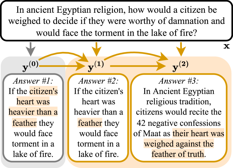
Figure 1: In contrast to the standard approach of mapping an input to an output in a single step (grey box), we propose a method that allows models to sequentially “reconsider” and update their predictions, i.e., the thought flow. In this (real) question answering example, the orange box marks our thought flow extension, which corrects a flawed answer in two steps.

In this paper, we propose the concept of a thought flow as a sequence of inter-dependent probability distributions. Furthermore, we propose a simple correction module to implement this concept. It can be used on top of any model that provides output logits of one or multiple distributions. In particular, it is inspired by the three moments of Hegel’s dialectics which it relates to forward and backward passes of the model and is trained to judge whether the predicted class distribution corresponds to a correct prediction.

In our experiments on question answering, we demonstrate our method’s ability to self-correct flawed answer span predictions and identify qualitative patterns of self-correction, such as span reductions/extensions. Figure 1 shows a real example of a thought flow that corrects a prediction ($\mathbf{y^{(0)}}$) that would be the output of a standard model to a new prediction ($\mathbf{y^{(2)}}$) within two steps, namely a shrinkage of the answer span and a cross-sentence answer jump. We find that our method can achieve performance improvements up to 9.6% $\text{F}_{1}$(absolute) on a question answering dataset.

Finally, we assess the impact of thought-flow predictions on human users within a crowdsourcing study. We find that thought-flow predictions are perceived as significantly more correct, understandable, helpful, natural, intelligent than single-answer predictions and/or top-3 predictions and result in the overall best user performance without increasing completion times or mental effort.

To sum up, our contributions are (i) a formalization of a thought flow inspired from human thinking and Hegel’s dialectics, (ii) a novel correction module and a corresponding gradient-based update scheme to generate a thought flow in a state-of-the-art transformer network, (iii) experiments on question answering that demonstrate its strong correction capabilities and identify qualitative patterns of self-correction, (iv) a crowdsourcing user study that demonstrates that thought flows can improve perceived system performance as well as actual user performance using the system.

2 Thought Flow Networks

In this section, we present background on Hegel’s dialectics (Section 2.1), formalize thought flows based on it (Section 2.2), and present a concrete implementation for question answering (Section 2.3).

2.1 Inspiration: Hegel’s Dialectics

To give models the opportunity to reflect and refine their predictions, we take inspiration from Hegel’s dialectics. Dialectics, in general, describes an argumentative method involving opposing sides Maybee (2020). What distinguishes Hegel’s dialectic from other dialectics is that in his dialectic, the opposing sides are views or definitions while, e.g., in Platon’s dialectic the opposing sides are people Maybee (2020). Besides its philosophical relevance, Hegel’s dialectics has been related to various fields before, such as cognitive sciences Riegel (1973), neuroscience Boonstra and Slagter (2019) or optimization Kadioglu and Sellmann (2009).

In the following, we will briefly introduce the three moments of Hegel’s dialectics and distinguish it from the thesis-antithesis-synthesis triad before we use them to derive our thought flow concept in the following section.

Three Moments.

Hegel’s dialectics distinguishes three moments: (i) the moment of understanding, (ii) the dialectical moment, and (iii) the speculative moment. The moment of understanding refers to the initial, “seemingly stable” view. In the second moment, this supposed stability is lost due to the view’s one-sidedness or restrictedness and the initial determination sublates itself into its own negation. The speculative moment unifies the first two determinations by negating the contradiction Maybee (2020).

Thesis-Antithesis-Synthesis Triads.

The three moments are often compared to a thesis-antithesis-synthesis triad, which was popularized by Heinrich Moritz Chalybäus, but cannot necessarily be equated to it as argued by, e.g., Mueller Mueller (1958). While the thesis-antithesis-synthesis triad can suggest the notion of a “one pass” process, the dialectical process in Hegel’s dialectic does not have to end after a single iteration, but can go through several iterations Maybee (2020). The possibility for iteration is an essential property of our thought flow

2.2 Formalization of Thought Flow Concept

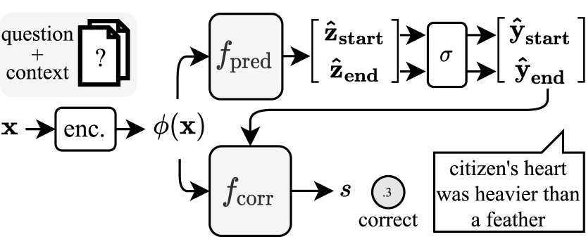
(a) First label and correctness prediction ($\rightarrow$ moment of understanding).

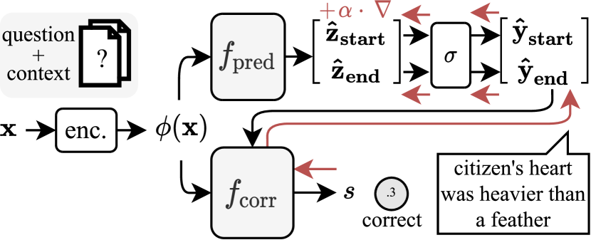
(b) Gradient calculation w.r.t. the label logits ($\rightarrow$ dialectical moment).

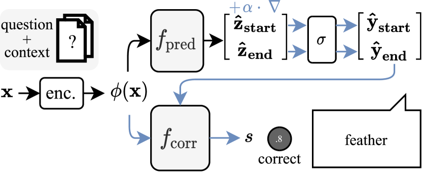
(c) Update logits and correctness score ($\rightarrow$speculative moment).

Figure 2: The steps of the prediction update scheme and their relation to the three moment of Hegel’s Dialectics. The example shows the first answer change from Figure 1.

We now translate the abstract description of these three moments into a simplified mathematical setting that can be implemented in any (neural) model that uses a vector-valued representation of the input (such as an embedding) and outputs (tuples of) logits. In particular, we embed Hegel’s dialectics in a framework of obtaining an initial “thought” vector and iteratively updating it in the three “moments”. Note that our formalization is not to be understood as an accurate reflection of Hegel’s dialectics but serves as a useful inspiration to enable the development of a novel machine learning model.

Thought.

We model a thought with $\mathbf{\hat{\mathbf{z}}}\in Z$, the logits corresponding to a model’s prediction and $Z\subseteq\mathbb{R}^{c}$ being the logit space. This $\mathbf{\hat{\mathbf{z}}}$ serves as a representation of the model’s “decision state” as it captures information about the most probable output as well as possible alternatives and uncertainty.

Moment of Understanding.

The first moment relates to an initial, seemingly stable view. We model this with the initial value of $\mathbf{\hat{\mathbf{z}}^{(0)}}$, obtained from applying the prediction function $f_{\text{pred}}:\Phi\rightarrow Z$ to the model to the encoded input $\phi(\mathbf{x})$ with an encoding function $\phi:\mathbb{R^{d}}\rightarrow\Phi$ and the encoding space $\Phi\subseteq\mathbb{R}^{e}$ (see Figure 2(a)).

Dialectical Moment.

In the second moment, the stability breaks down due to the view’s one-sidedness or restrictedness. To model this, we first introduce a new function $f_{\text{corr}}:Z\times\Phi\rightarrow\mathbb{R}$ that differentiably maps $\mathbf{\hat{\mathbf{z}}^{(0)}}$ to a correctness score $s\in\mathbb{R}$ that is an estimate of the quality of the model prediction corresponding to $\mathbf{\hat{\mathbf{z}}^{(0)}}$ while being conditioned on $\phi(\mathbf{x})$. Intuitively, $f_{\text{corr}}(\mathbf{\hat{\mathbf{z}}^{(0)}},\phi(\mathbf{x}))$ scores how good the current prediction corresponding to $\mathbf{\hat{\mathbf{z}}^{(0)}}$ is given the model input corresponding to $\phi(\mathbf{x})$. Next, we formalize the dialectical moment with the gradient of the correctness score with respect to $\mathbf{\hat{\mathbf{z}}^{(0)}}$, i.e. $\nabla^{T}_{\mathbf{\hat{\mathbf{z}}}^{(0)}}s$ (see Figure 2(b)). Thus, we ask “How does the thought $\mathbf{\hat{\mathbf{z}}^{(0)}}$ have to change in order to be more correct?” This gradient represents the view’s instability: As it creates a tension away from the current $\mathbf{\hat{\mathbf{z}}^{(0)}}$ towards a new one, it destroys its stability and thus negates the initial view.

Speculative Moment.

The third moment unites the initial view with the negation from the dialectical moment. We formalize this by modifying $\mathbf{\hat{\mathbf{z}}^{(0)}}$ with a step into the gradient’s direction that yields

$$\mathbf{\hat{\mathbf{z}}^{(1)}}:=\mathbf{\hat{\mathbf{z}}^{(0)}}+\alpha^{(0)}\cdot\nabla^{T}_{\mathbf{\hat{\mathbf{z}}}^{(0)}}s$$ (1)

where $\alpha^{(0)}$ is a, potentially dynamic, step width and $\mathbf{\hat{\mathbf{z}}^{(1)}}$ again constitutes the subsequent first moment of the next iteration (see Figure 2(c)).

Iteration.

Iterative application of the dialectical and the speculative moment yields a sequence of logits $\left(\mathbf{\hat{\mathbf{z}}^{(k)}}\right)_{k=0}^{N}$ and predictions $\left(\mathbf{\hat{\mathbf{y}}^{(k)}}\right)_{k=0}^{N}$.

In the following, we concretize this abstract formalization for the example of question answering.

2.3 Implementation in Transformers for QA

Figure 2 visualizes our formalization for the question answering example introduced in Figure 1. We now discuss QA-related implementation details.

2.3.1 Choosing Parameters and Functions

To apply our abstract thought flow method to a real model we have to (a) determine how we structure the model prediction logit vector $\mathbf{\hat{\mathbf{z}}}$, (b) choose an input representation $\phi(\mathbf{x})$ (that is passed to $f_{\text{pred}}$ as well as $f_{\text{corr}}$), (c) choose a parametrization of the correctness score prediction function $f_{\text{corr}}$ and (d) define what the correctness score $s$ measures. In the following, we describe how these aspects can be realized in a transformer-based QA model.

Composing $\mathbf{\hat{\mathbf{z}}}$.

In extractive QA, a typical approach to model answer span extraction from a context of $L$ tokens, is to use two probability distributions: (i) $\mathbf{\hat{\mathbf{y}}}_{\text{start}}\in[0,1]^{L}$ that assigns a probability of being the start of the answer to each token in the context and (ii) a respective end token distribution $\mathbf{\hat{\mathbf{y}}}_{\text{end}}\in[0,1]^{L}$. To match our previously defined formalization, we define $\mathbf{\hat{\mathbf{z}}^{(i)}}:=\begin{bmatrix}\mathbf{\hat{\mathbf{z}}_{\text{start}}^{(i)}}&\mathbf{\hat{\mathbf{z}}_{\text{end}}^{(i)}}\end{bmatrix}^{\text{T}}$ which is linked to the respective probability distributions via the softmax function $\sigma$:

$$\mathbf{\hat{\mathbf{y}}^{(i)}}:=\begin{bmatrix}\mathbf{\hat{\mathbf{y}}_{\text{start}}^{(i)}}&\mathbf{\hat{\mathbf{y}}_{\text{end}}^{(i)}}\end{bmatrix}^{\text{T}}=\begin{bmatrix}\sigma(\mathbf{\hat{\mathbf{z}}_{\text{start}}^{(i)}})&\sigma(\mathbf{\hat{\mathbf{z}}_{\text{end}}^{(i)}})\end{bmatrix}^{\text{T}}.$$

Input Representation $\phi(\mathbf{x})$.

In contrast to transformer-based classification models that usually rely on the embedding of the [CLS] token, typical transformer-based QA models apply a linear function on top of each token’s embedding that maps the embedding to a start and an end logit. To represent the input, we thus need a choice of $\phi(\mathbf{x})$ that captures the relevant parts of the (potentially very long) input. We choose a weighted average over all token embeddings. As weights, we choose the element-wise product of the predicted start and end probabilities. We thus define $\phi(\mathbf{x})\in\mathbb{R}^{d}$ with $d$ denoting the dimension of the embeddings as:

$$\mathbf{\tilde{w}^{(i)}}:= \left(\mathbf{\hat{\mathbf{y}}_{\text{start}}^{(i)}}\odot\mathbf{\hat{\mathbf{y}}_{\text{end}}^{(i)}}+\epsilon\cdot\mathbf{1}\right) \in\mathbb{R}^{L}$$ (2)

$$\phi(\mathbf{x})^{(i)}:= \left[e_{1},e_{2},...,e_{L}\right]\cdot\frac{\mathbf{\tilde{w}^{(i)}}}{\Sigma_{j}\mathbf{\tilde{w}^{(i)}}_{j}} \in\mathbb{R}^{d}$$ (3)

where $\epsilon$ is a small constant that ensures that we do not divide by zero, $e_{i}$ is the embedding of the $i$-th token and $\odot$ is element-wise multiplication. The intuition behind this is that the correction module should have access to all information about the context that the prediction model focused on.

Choosing $f_{\text{corr}}$.

We use a two-layer MLP with SELU activation Klambauer et al. (2017) to map the concatenated vector

$$\begin{bmatrix}\text{dropout}(\phi(\mathbf{x})^{(i)})&\mathbf{\hat{\mathbf{z}}^{(i)}_{\text{start}}}&\mathbf{\hat{\mathbf{z}}^{(i)}_{\text{end}}}\end{bmatrix}^{\text{T}}\in\mathbb{R}^{d+2\cdot L}$$ (4)

to a correctness score $s$. Note that $f_{\text{corr}}$ does not receive the decoded answer text but directly uses the start and end logits to provide differentiability.

Correctness Score $s$.

Following standard evaluation metrics for question answering, we use the $\text{F}_{1}$-score of the predicted answer as the correctness score that $f_{\text{corr}}$ is trained to predict.

2.3.2 Training

To train $f_{\text{corr}}$, we freeze the parameters of $f_{\text{pred}}$. Then, we pass the training instances through the whole model (including $\phi$, $f_{\text{pred}}$ and $f_{\text{corr}}$) as shown in Figure 2(a) to obtain the predicted correctness score $s$ (i.e., $f_{\text{corr}}$ predicts an $\text{F}_{1}$-score estimate without access to the ground-truth answer span). We determine the ground-truth correctness score by calculating the $\text{F}_{1}$-score between the ground truth answer and the answer prediction from $f_{\text{pred}}$. We define the correction prediction loss as the mean squared error between the calculated score and the predicted $s$ and train $f_{\text{corr}}$ to minimize it.

2.3.3 Inference

At inference time, we encode a new input and predict (i) the answer start and end logits using $f_{\text{pred}}$ and (ii) an estimated $\text{F}_{1}$-score $s$ of the predicted answer span using the correction module $f_{\text{corr}}$ as shown in Figure 2(a). Instead of directly using the initial logits as the model’s prediction — as would be done in a standard model — we iteratively update the logits w.r.t. the estimated correctness score’s gradient following our formalization from Section 2.2 as shown in Figures 2(b) and 2(c).

Update Rule.

As described in Section 2.2, we aim at modifying $\mathbf{\hat{\mathbf{z}}}^{(i)}$ such that the correction module assigns an increased correctness (i.e., $\text{F}_{1}$-score in this application to QA). To apply Equation 1, we have to define how the step size $\alpha$ is chosen in our QA application. We choose a time-independent $\alpha$ such that a predefined probability mass $\delta$ is expected to move. To this end, we first take a probing step of length one, calculate the distance as the $L_{1}$ norm between the initial distribution and the probe distribution and choose the step width $\alpha\in\mathbb{R}^{+}$ such that it scales the linearized distance to the hyperparameter $\delta$:

$$\alpha:=\left[\frac{\delta}{||\sigma(\mathbf{\hat{\mathbf{z}}}^{(i)})-\sigma(\mathbf{\hat{\mathbf{z}}}^{(i)}+\nabla^{T}_{\mathbf{\hat{\mathbf{z}}}^{(i)}}s)||_{1}+\epsilon}\right]$$ (5)

where $\sigma(\cdot)$ denotes the softmax function and $\epsilon\in\mathbb{R^{+}}$ is a small constant for numerical stability.

Monte Carlo Dropout Stabilization.

The gradient $\nabla_{\mathbf{\hat{\mathbf{z}}}^{(i)}}s$ is deterministic but can — as we find in preliminariy experiments — be sensitive to small changes in the input representation $\phi(\mathbf{x})$. We therefore stabilize our correction gradient estimation by sampling and averaging gradients instead. For this, we use the dropped-out input encoding from Equation 4 and sample five gradients for every step using MCDrop Gal and Ghahramani (2016).

3 Question Answering Experiments

3.1 Data, Model and Training

Dataset.

We choose the HotpotQA dataset (distractor setting) Yang et al. (2018) to evaluate our models because it contains complex questions that require multi-hop reasoning over two Wikipedia articles. In the distractor setting, the model is “distracted” by eight irrelevant articles that are passed to the model in addition to the two relevant articles. In addition to yes/no/answer span annotations, HotpotQA also provides explanation annotations in the form of binary relevance labels over the paragraphs of the relevant articles which we do not use when training our models. As the public test set is secret, we use the official validation set as test set and sample a custom validation set of size 10k from the training set leaving 80,564 training instances.

Base model.

We use a Longformer-large Beltagy et al. (2020) model with a linear layer on top that maps token embeddings to start and end logits as our underlying question answering model. The model reaches 63.5% $\text{F}_{1}$ (SD=0.6) on the HotpotQA validation set averaged over three random seeds and can handle input lenghts up to 4096 tokens which enables us to feed-in the entire context as a single instance without truncation. The model’s input is a single token sequence that contains the question followed by the answer context (i.e., the 10 concatenated Wikipedia articles). The model’s output are two distributions over the input tokens (i.e., two 4096-dimensional distributions), one for the answer start position and one for the answer end position. This allows the model to choose its answer from any text span within the context. We prepend a “yes” and a “no” token to the context, that offers the advantage of modeling these answer options within the same distributions as the text span answers. In total, this model has 435M parameters compared to the additional 331k parameters our MLP implementation of $f_{\text{corr}}$ adds.

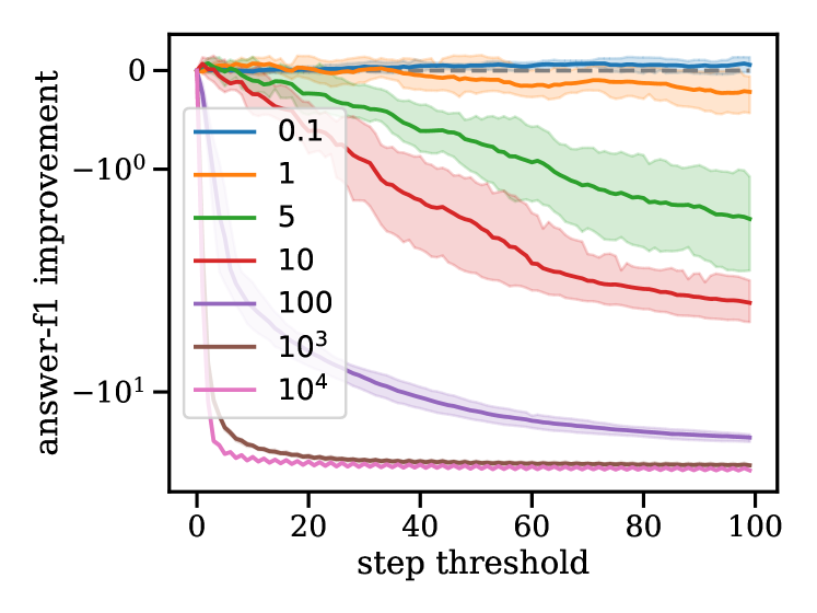
(a) Non-oracle-stopped flows.

(b) Oracle-stopped flows.

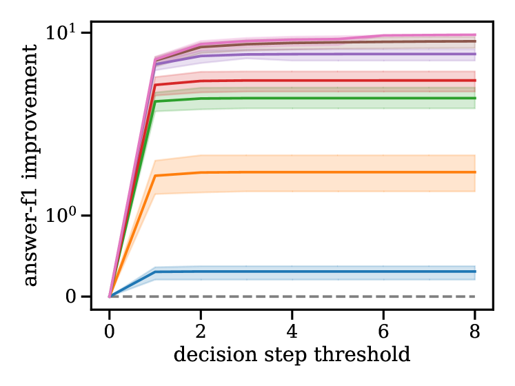
(c) Oracle-stopped flows per decision change.

Figure 3: Thought flows with different gradient scaling targets $\delta$ averaged over three seeds of a question answering model. Higher values for $\delta$ correspond to more aggressive decision changes. Without a stopping oracle that stops when the thought flow does no longer improve an answer (left), only $\delta=0.1$ provides consistently stable, but very small F1 improvements. With an oracle (middle), higher values for $\delta$ reach higher and faster F1 improvements up to $>$9%. Nearly all performance gains are achieved by the first decision change (right). y axes use a symlog scale. Improvements are reported as absolute F1 scores (not relative to the the base performance).

Training Details.

We first train the base models on for five epochs on a single V100 GPU using a learning rate of $10^{-5}$, an effective batch size of 64 using an AdamW optimizer Loshchilov and Hutter (2019), early stopping and a cross entropy loss on the start/end logits. We subsequently train the correction modules using the same setting but the mean squared error loss function for $\text{F}_{1}$-score prediction training. Training one model each took approximately three days. In the following, we report all results as averages over three random seeds including standard deviations.

3.2 Performance Improvements

How does Performance Vary Over Steps?

Figure 3(a) shows how $\text{F}_{1}$-scores per gradient scaling target $\delta$ evolve over 100 steps. We observe that small $\delta$ values enable small $\text{F}_{1}$ improvements. While $\delta=0.1$ consistently improves $\text{F}_{1}$-scores, all other $\delta$ values eventually deteriorate $\text{F}_{1}$-scores. The higher the $\delta$ value, the quicker the $\text{F}_{1}$ decrease. We conclude that (i) very small $\delta$ values are not sufficient to reach notable performance gains and that (ii) larger $\delta$ can initially improve performance but then “overshoot” with their corrections. We hypothesize that a remedy to this trade-off is to use larger $\delta$ values but stop the corresponding flows at the right time.

What if We Had a Stopping Oracle?

To test this hypothesis, we introduce an oracle stopping function that stops the thought flow where it achieves it best $\text{F}_{1}$ performance. Figure 3(b) shows that, with this oracle function, thought flows can reach performance improvements up to 9.6% $\text{F}_{1}$(SD=0.61).

Figure 3(c) shows that almost all performance improvements are due to the first decision change within the thought flows and answer spans constantly improve and do not randomly shift across the context. This observation shows that single thought flow changes are highly effective and can reach substantial corrections fast.

Pattern	Frequ.	Example
cross-sentence	52.7%	Question: Who is older Danny Green or James Worthy?
		(1) Daniel Richard ”Danny” Green, Jr. (born June 22, 1987) is an American professional basketball player for the San Antonio Spurs of the National Basketball Association (NBA).
		(2) James Ager Worthy (born February 27, 1961) is an American professional basketball coach and former player, commentator, television host, and analyst.
span reduction	23.3%	Question: What philosophy related to creationism is Paul Nelson noted for?
		(1) Paul A. Nelson (born 1958) is an American philosopher of science noted for his advocacy of young earth creationism and intelligent design
		(2) Paul A. Nelson (born 1958) is an American philosopher of science noted for his advocacy of young earth creationism and intelligent design
span extension	21.3%	Question: Ronald Reagan and George H. W. Bush both held which position in office?
		(1) The presidency of Ronald Reagan began on January 20, 1981, when Ronald Reagan was inaugurated as President of the United States, and ended on January 20, 1989.
		(2) The presidency of Ronald Reagan began on January 20, 1981, when Ronald Reagan was inaugurated as President of the United States, and ended on January 20, 1989.
in-sent.	7.3%	Question: When was the stadium that held the 2015 Magyar Kupa demolished?
		(1) The stadium was closed in 2016 and demolished in 2017 to give place to the new Ferenc Puskas Stadium.
		(2) The stadium was closed in 2016 and demolished in 2017 to give place to the new Ferenc Puskas Stadium.
logic hops	4%	Question: Is the Pakistan fast bowler who joined the Kent County Cricket Club in June, 2011 a left-hand or right-hand batsmans?
		(1) Wahab Riaz (Punjabi, Urdu: ; born 28 June 1985) is a Pakistani cricketer.
		(2) He is a left-arm fast bowler and a right-hand batsman.

Table 1: A subset of correction Patterns identified in 150 randomly sampled thought flows using $\delta=1$. The correct answer is marked bold, the predicted answer per flow step is marked in orange. We provide the full list of identified patterns in the appendix.

3.3 Thought Flow Patterns

In a qualitative evaluation, we identify thought flow patterns. We randomly sample 150 instances from the subset of the official validation split for which the thought flow changed the initial answer prediction. We identify six (non-exclusive) correction patterns and show selected examples in Table 1.

Cross-Sentence.

With 52.7%, this is the most frequent type of correction. The thought flow shifts the predicted answer from one sentence to another.

Span Reduction.

The thought flow can shorten the predicted answer span to correct the answer.

Span Extension.

Similarly, the thought flow can also enlarge a predicted answer span to correct it.

In-Sentence.

On top of in-sentence span reduction/extension, the thought flow can also jump between non-overlapping spans within a sentence.

Entity Refinement.

In this correction pattern, the though flow keeps predicting the same entity but jumps to an alternative mention of the entity.

Logic Hops.

The thought flow performs a step-wise reasoning that first resolves the first step of HotpotQA’s two-step reasoning structure before jumping to the second step, i.e., the correct answer.

Combinations.

We observe various combinations of the aforementioned patterns. A model can, for instance, jump between sentences, refine entities and reduce the answer span.

Corrections can also occur sequentially. We provide detailed examples in the appendix. We additionally observe flow patterns with very high number of decision changes. These typically correspond to two- or three-cycles between answer spans or exhibit a seemingly chaotic behavior.

4 Human Evaluation

While the previous section showed that thought flows can enable complex self-correction and can reach promising performance gains, we now investigate how thought flow predictions affect human users in an AI-assisted question answering task.

4.1 Experiment Design

We choose a within-subject design in which each participant is exposed to three variations of a question answering system.

Conditions.

We aim at assessing the effect of the thought flow concept on users and therefore present the outputs of the oracle-stopped thought flow in one condition (TF) and compare it to two baseline conditions. As baselines, we use top-1 predictions (single) (to compare against standard models) and top-3 predictions (top-3) (to compare to an alternative approach to show several predictions). For all conditions, we present the predicted answer(s) along with the sentence in which they appear in the context.

Dependent Variables.

We study the effect of the condition (single, TF and top-3) on a set of dependent variables. We include variables on a per-question level (after each question) and on a per-system level (after all questions of one condition). The per-question variables include: (i) human answer correctness, (ii) perceived model correctness (iii) perceived understanding, (iv) perceived helpfulness and (v) completion time. The per-system variables include: (vi) usability using the UMUX questionnaire Finstad (2010, 2013), (vii) mental effort using the Paas scale Paas (1992), (viii) anthropomorphism using the respective subscale of the Godspeed questionnaire Bartneck et al. (2009), (ix) perceived intelligence using the subscale from the same questionaire, (x) average completion time. We provide a list of all questionnaires in the appendix.

Apparatus.

We sample 100 instances from the HotpotQA validation instances for which a thought flow using $\delta=1$ causes at least one prediction change. From these, we sample 30 instances per participant and randomly assign the instances to three bins of 10 questions (one bin per condition). We balance the six possible condition orders across participants and include three attention checks per participant. We provide screenshots of the study interface in the appendix.

4.2 Quantitative Results

We use MTurk to recruit US crowdworkers with $>$90% approval rate and the MTurk Masters qualification an collect responses from 55 workers.

4.2.1 Statistical Models.

Per-System Ratings.

We analyze the per-system ratings using Friedman tests to account for the paired responses due to the within-subject design. We use Holm-corrected Conover post hoc tests to identify significant pairwise differences.

Per-Item Ratings.

Note that the within-subject design of our study possibly introduces inter-dependencies within ratings that we have to account for using an appropriate statistical model. Additionally, our dependent variables are measured on different levels, e.g., completion time is measured on a ratio scale while human answer correctness is measured on a nominal (dichotomous) scale. We therefore use (generalized) linear mixed models (GLMM) and cumulative link mixed models (CLMM) to (i) account for random effects of question and subject IDs, and (ii) account for the variables’ respective measurement scales. We use LRT tests between the full model and the model without the condition variable to identify main effects of the condition variable and conduct Holm-corrected Tukey post-hoc tests.

Condition	perceived quality							user performance
	correct∗	understand∗	helpful∗	usability	mental effort	humanlike∗	intelligent∗	time∗	answer F1∗
single	A	A	A			A	A		A
top-3	A							B	B
TF

Table 2: Statistical results of our human evaluation ($N=55$). “^∗” marks dependent variables on which a significant effect of the system condition was observed (Friedman tests and LRT tests for GLMM/CLMM). Pairwise differences between conditions (Holm-adjusted Tukey/Conover tests) are reported as compact letter display codings. E.g., the “humanlike” column shows that the post hoc test detected a significant difference between single and TF but no significant difference between any other pair. Similarly, the last column shows pairwise differences between all conditions and the TF condition reaches significantly higher human answer $\text{F}_{1}$-scores than any other conditions. Variables for which TF is among the best performing models are marked cyan, variables for which it is found to be the sole superior system are marked green.

4.2.2 Results.

We find significant differences for all dependent variables except usability and mental effort. We summarize the results of our statistical analysis in Table 2 using CLD codings Piepho (2004). We provide the detailed $p$ values for main efects and each pairwise comparison in the appendix. In the following we discuss our findings for each dependent variable for which we found a significant main effect.

Perceived Answer Correctness.

While there is no statistically significant difference between showing users single answers or top-3 predictions, displaying thought flows leads to significantly higher answer correctness ratings.

Understanding.

Top-3 as well as thought flow predictions significantly increased the feeling understanding how the system came up with its answer compared to single predictions.

Helpfulness.

Similarly, top-3 and the thought flow predictions significantly improve perceived system helpfulness compared to single predictions.

Anthropomorphism.

While we observe no signficant difference in antropomorphism ratings between single and top-3 predictions, the thought flow predictions are perceived significantly more human-like/natural than the single answers.

Perceived intelligence.

Both, top-3 and the thought flow predictions, lead to an significantly increased perceived system intelligence.

Completion Time.

We observe that the top-3 predictions significantly improve completion times compared to single answers, but there is no significant increase for thought flows.

User Performance.

While top-3 predictions already improve user performance in terms of $\text{F}_{1}$-score of the user’s given answer, thought flow predictions enable even higher performances, that are significantly higher than answers given in the single answer or top-3 conditions. We additionally analyze user answers using exact match scores and find the same effects and model orders.

Overall, our results indicate that thought flows are better or equally good than single answer or top-3 predictions regarding all evaluated dimensions. In particular for perceived answer correctness, humanlikeness and user performance, thought flows are significantly better than both, the single answers and the top-3 predictions. While comparable (statistically indistinguishable) improvements of understanding, helpfulness, naturalness and intelligence can also be achieved using top-3 predictions, these come at the cost of significantly increased completion times compared to single answers. In contrast, we do not find a significant time increase using thought flows.

5 Related Work

Cognitive Modeling and Systems.

The fields of cognitive modeling and cognitive systems provide numerous models of human thinking Rupert (2009); Busemeyer and Diederich (2010); Levine (2018); Lake et al. (2017). While work in these fields often orients towards accurate descriptions of human cognition, our method does not aim to provide a plausible description of cognitive process but, instead, aims to apply a philosophical concept to machine learning in order to improve classification performance and user utility.

Confidence Estimation and Model Corrections.

Estimating a model’s confidence and the correctness of its predictions is addressed with various methods, including the training of secondary models for predicting the main model’s uncertainty Blatz et al. (2004); DeVries and Taylor (2018). Among those, ConfidNet is particularly related to our approach as it predicts the true-class probability of the main model Corbière et al. (2019). In contrast, our correction module receives the class probabilities of the main model as an input and predicts a correctness score. In difference to methods aiming at estimating accurate confidence scores, we predict such scores only as an auxiliary task in order to generate a gradient that allows us to update the model prediction. Regarding model correction, the arguably most established approach to learn corrections of model predictions is gradient boosting Friedman (2001) including its popular variant XGBoost Chen and Guestrin (2016). In contrast to those works, we do not use an ensemble of weak learners but propose a lightweight correction module that is applicable on top of any existing classification model. Further, in our method, the correction module receives the main model’s predictions and is able to directly adapt them.

Sequences of Predictions.

The idea of iteratively predicting and correcting has been explored for a long time. Early work includes Mori et al. who present a non-neural iterative correction method tailored to estimate elevation maps from aerial stereo imagery Mori et al. (1973). Katupitiya et al. propose to iterate two neural networks to address the problem of predicting inputs of a mechanical process given the outputs of the process Katupitiya and Gock (2005). While their method is specifically designed for the task of input prediction, our work presents a general-purpose classification model that iterates class label predictions. Besides those task-specific methods, there are models and inference methods that make use of an iterative prediction process by design, such as Hopfield networks Hopfield (1982) and their modern variants Barra et al. (2018); Ramsauer et al. (2020), or Loopy Belief Propagation, Markov Chain Monte Carlo or Gibbs sampling Bishop (2006); Koller and Friedman (2009). While these techniques can be linked to our work conceptually, they all require to train a new model. In contrast, our approach can be applied to an existing neural model as well. Another related approach is chain-of-thought prompting Wei et al. (2022) in which a language model is prompted with demonstrations of problem decomposition/reasoning in a few-shot manner and subsequently can be observed to show similar behavior in its answer. While this method yields impressive model answers, it predicts one answer that contains information on its deduction without changing or correcting its answer. In contrast, our method is not targeted towards decomposition/reasoning but predicts a sequence of answers with the goal of iteratively improving it.

Learning to Stop.

A further line of work, ACT Graves (2016) and PonderNet Banino et al. (2021), trains recurrent networks to learn when to stop applying recurrent transformations within the model. While their approaches require the model to contain recurrent modules and to retrain the base model, our method only requires the model to yield output logits and leaves the base model unchanged.

6 Conclusion

In this paper, we introduced a task-agnostic self-correction formalism that turns a model’s single output prediction into an evolving sequence of predictions—the thought flow. We take inspiration from Hegel’s dialectics and propose a correction module along with a gradient-based update rule that sequentially updates a model’s output distributions in the direction of an increasing self-estimate of correctness. We apply our method to question answering models and conduct extensive experiments including human evaluation. We find that thought flows (i) can increase $\text{F}_{1}$-scores up to 9.3%, (ii) exhibit complex self-correction patterns and (iii) provide significant improvements in human interaction and system perception including task performance and perceived system correctness and naturalness. A potential next step to further improve performance is learning to stop.

Appendix A Question Answering Experiments

A.1 Dataset Details.

We use the HotpotQA dataset Yang et al. [2018], which is an English multi-hop question answering data set. It covers 90,564 training instances, 7,405 test validation instances and 7,405 test instances per setting (there are a distractor and a fullwiki setting). Training instances are grouped by difficulty and cover 18,089 easy, 56,814 medium and 15,661 hard questions. We refer to Yang et al. [2018] for more details.

Pattern	Frequ.	Example
cross-sentence	52.7%	Question: Who is older Danny Green or James Worthy?
		(1) Daniel Richard ”Danny” Green, Jr. (born June 22, 1987) is an American professional basketball player for the San Antonio Spurs of the National Basketball Association (NBA).
		(2) James Ager Worthy (born February 27, 1961) is an American professional basketball coach and former player, commentator, television host, and analyst.
span reduction	23.3%	Question: What philosophy related to creationism is Paul Nelson noted for?
		(1) Paul A. Nelson (born 1958) is an American philosopher of science noted for his advocacy of young earth creationism and intelligent design
		(2) Paul A. Nelson (born 1958) is an American philosopher of science noted for his advocacy of young earth creationism and intelligent design
span extension	21.3%	Question: Ronald Reagan and George H. W. Bush both held which position in office?
		(1) The presidency of Ronald Reagan began on January 20, 1981, when Ronald Reagan was inaugurated as President of the United States, and ended on January 20, 1989.
		(2) The presidency of Ronald Reagan began on January 20, 1981, when Ronald Reagan was inaugurated as President of the United States, and ended on January 20, 1989.
in-sent.	7.3%	Question: When was the stadium that held the 2015 Magyar Kupa demolished?
		(1) The stadium was closed in 2016 and demolished in 2017 to give place to the new Ferenc Puskas Stadium.
		(2) The stadium was closed in 2016 and demolished in 2017 to give place to the new Ferenc Puskas Stadium.
entity refin.	8%	Question: Which host of Sunday Night Safran has the hebrew first name Yehoshua?
		(1) John Michael Safran (Hebrew: ”Yehoshua Safran” ; born 13 August 1972) is an Australian radio personality, satirist, documentary maker and author, known for combining humour with religious, political and ethnic issues.
		(2) It was hosted by John Safran and Catholic priest, Bob Maguire.
logic hops	4%	Question: Is the Pakistan fast bowler who joined the Kent County Cricket Club in June, 2011 a left-hand or right-hand batsmans?
		(1) Wahab Riaz (Punjabi, Urdu: ; born 28 June 1985) is a Pakistani cricketer.
		(2) He is a left-arm fast bowler and a right-hand batsman.
combined	9.3%	Question: Who was born in 1922 and published a book in 1985 by Delacorte Press?
		(1) Kurt Vonnegut Jr. (November 11, 1922; April 11, 2007) was an American writer.
		(2) Galapagos is the eleventh novel written by American author Kurt Vonnegut.

Table 3: Correction Patterns identified in 150 randomly sampled thought flows using $\delta=1$. The correct answer is marked bold, the predicted answer per flow step is marked in orange.

Examples
Question: How many times did the man who coached the 1986-87 UNLV Runnin’ Rebels fail to win 20 games in a season?
(1) He spent the majority of his career coaching with the UNLV Runnin’ Rebels, leading them four times to the Final Four of the NCAA Men’s Division I Basketball Tournament, winning the national championship in 1990.
(2) Overall, he won over 700 games in his career, and only twice failed to win 20 games in a season.
(3) Overall, he won over 700 games in his career, and only twice failed to win 20 games in a season.
Question: Why did the CEO of the football team based in Denver, Colorado step down in 2014?
(1) He served as the Broncos CEO from his purchase of the club in 1984 until July 2014, when he stepped down as Broncos’ CEO due to the onset and progression of Alzheimer’s disease.
(2) He served […], when he stepped down as Broncos’ CEO due to the onset and progression of Alzheimer’s disease.
(3) He served […], when he stepped down as Broncos’ CEO due to the onset and progression of Alzheimer’s disease.

Table 4: Multi-step correction examples ($\delta=1$).

A.2 Thought Flow Patterns

We provide an extended list of patterns and examples from our qualitative thought flow analysis in Table 4. In addition Table 4 shows additional thought flow examples using three correction steps.

Appendix B User Study

B.1 Questionnaire Items

B.1.1 Per-System Questionnaires

Usability.

The UMUX usability scale Finstad [2010, 2013] uses the following four 5-point Likert items:

• This system’s capabilities meet my requirements.

• Using this system is a frustrating experience.

• This system is easy to use.

• I have to spend too much time correcting things with this system.

Mental Effort.

The Pass mental effort scale usability scale Paas [1992] uses a single 9-point Likert item:

• Please rate the mental effort required to decide if the system’s answer is correct. (The 9 points are labeled from “very, very low mental effort” to “very, very high mental effort”.)

Anthropomorphism.

The Godspeed anthropomorphism subscale Bartneck et al. [2009] use five 5-point semantic differential scales that ask the user to rate the system in a spectrum of:

• fake – natural

• machinelike – humanlike

• unconscious – conscious

• artificial – lifelike

• (moving rigidly – moving elegantly) (We exclude this item as it is not applicable to question answering systems.)

Perceived Intelligence.

The Godspeed perceived Intelligence subscale Bartneck et al. [2009] use five 5-point semantic differential scales that ask the user to rate the system in a spectrum of:

• incompetent – competent

• ignorant – knowledgeable

• irresponsible – responsible

• unintelligent – intelligent

• foolish – sensible

B.1.2 Per-Item Questionnaires

Perceived Answer Correctness.

We use a single binary item to collect perceived answer correctness ratings:

• I think the system’s answer is correct.

Perceived Helpfulness.

We use a single 5-point Likert item to collect helpfulness ratings:

• I think the system’s answer enables me to give the correct answer.

Perceived Understanding.

We use a single 5-point Likert item to collect understanding ratings:

• I understand how the system came up with its answer.

B.2 Interface

Figures 4, 5 and 6 show screenshots of our experiment interface for the three studied prediction conditions TF, top-3 and single. Figure 7 depicts an attention check question.

B.3 Statistical Results

Table 5 provides the $p$ values for main effects and each pairwise comparison.

	perceived quality							user performance
	correct∗	understand∗	helpful∗	usability	mental effort	humanlike∗	intelligent∗	time∗	answer F1∗
Main effect	$<$0.0001	$<$0.0001	$<$0.0001	0.07968	0.6282	0.03575	0.00124	$<$0.0001	$<$0.0001
tf – single	$<$0.0001	$<$0.0001	$<$0.0001	0.13116	1	0.03431	0.00586	0.15304	$<$0.0001
tf – top-3	0.00891	0.8867	0.9994	0.84254	1	0.30556	1	0.06207	$<$0.0001
top-3 – single	0.51897	$<$0.0001	$<$0.0001	0.13653	1	0.25097	0.00586	0.00012	$<$0.0001

Table 5: Detailed $p$ values for all main effects and pairwise comparisons shown in Table 2. Significant $p$ values are marked bold. Cell colors follow the color coding on Table 2.

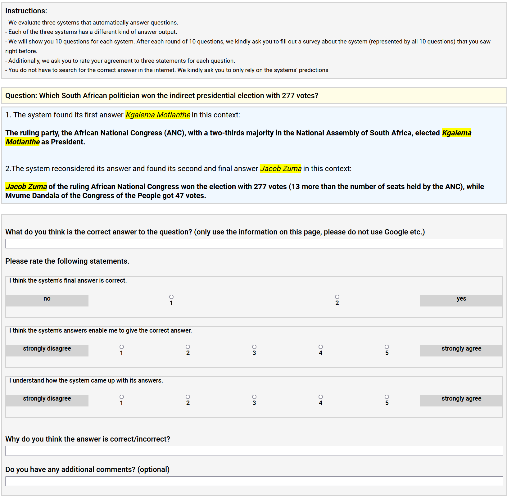
Figure 4: User study interface showing the TF condition (ours).

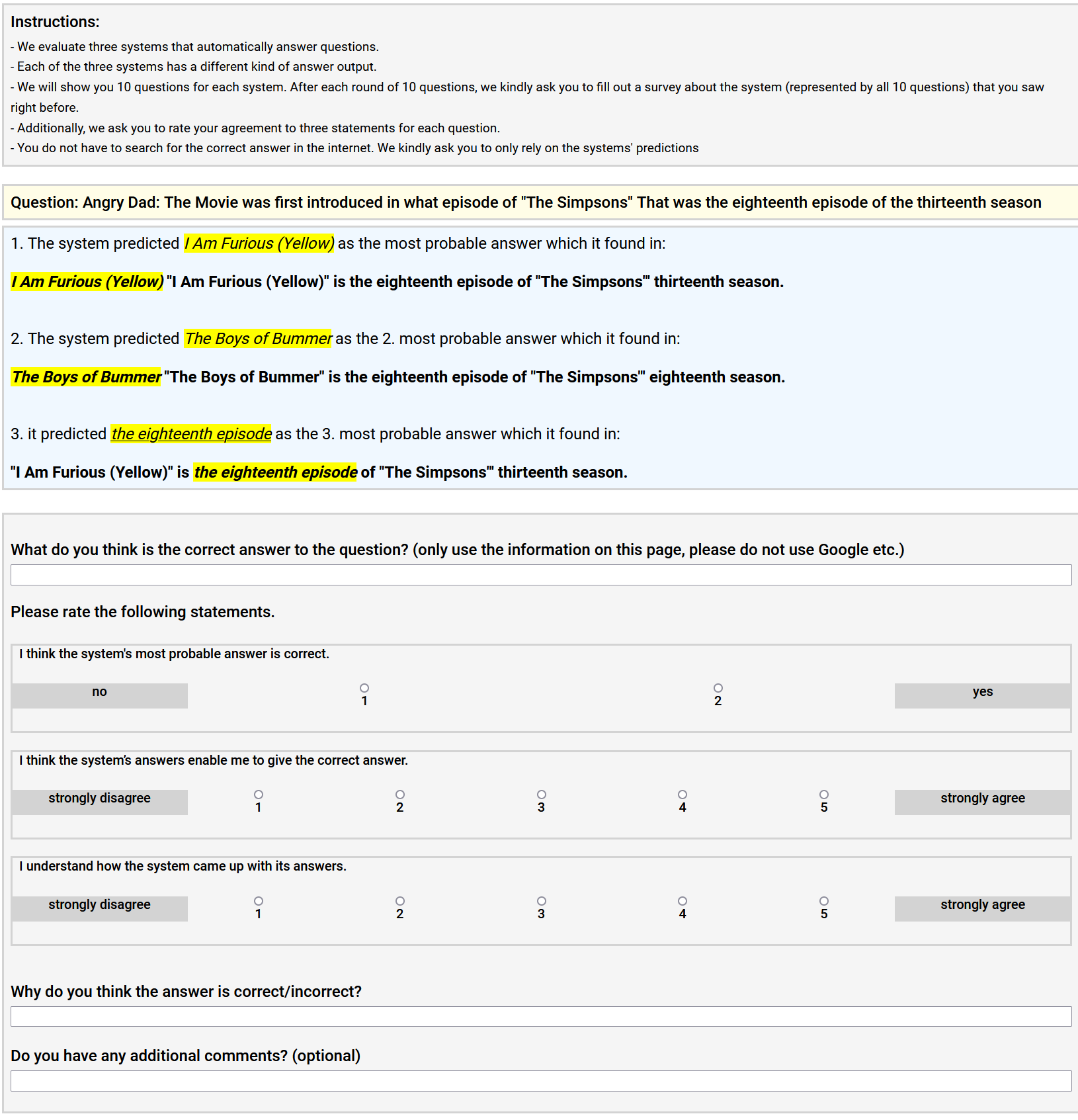
Figure 5: User study interface showing the top-3 condition.

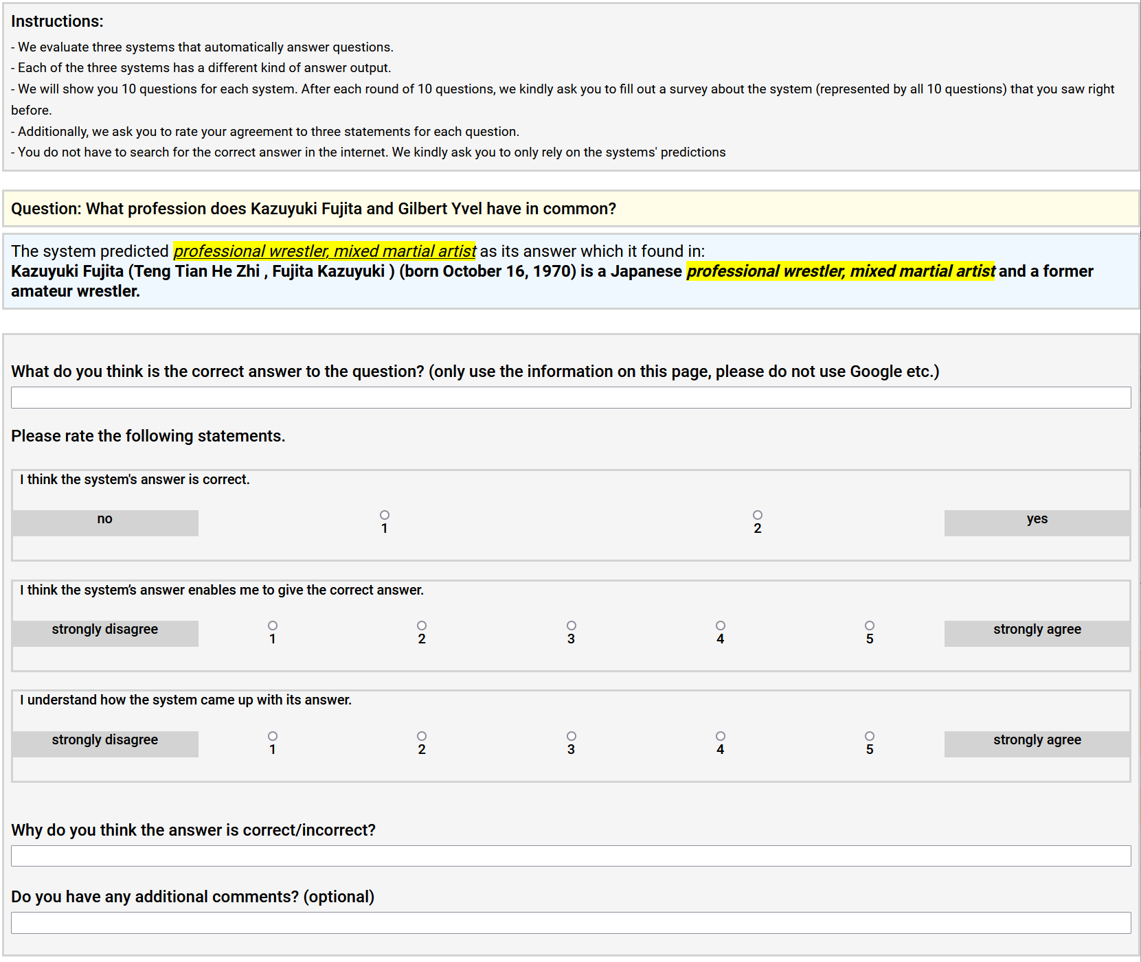
Figure 6: User study interface showing the single condition.

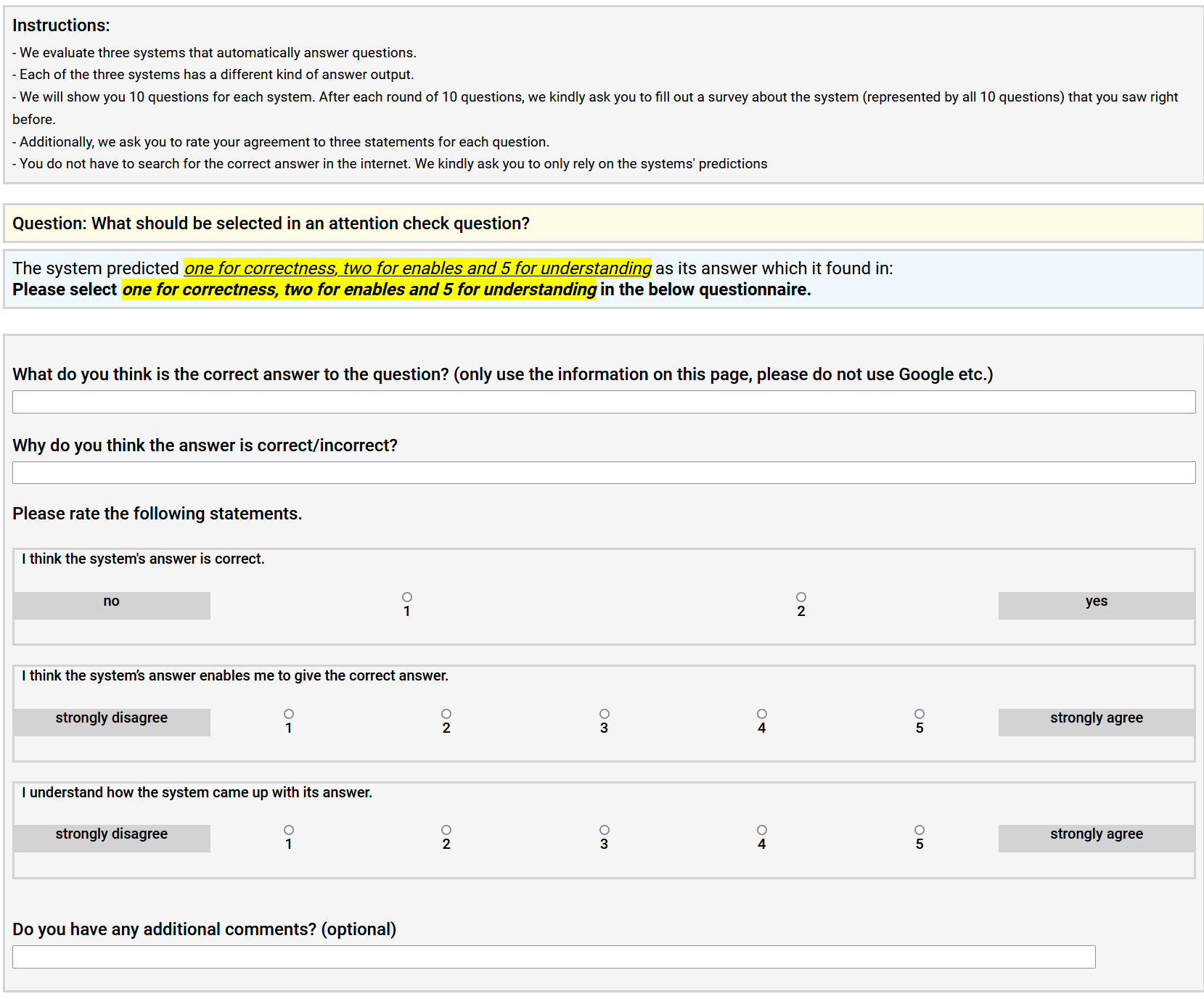
Figure 7: User study interface showing an attention check.

References

- Banino et al. [2021] Andrea Banino, Jan Balaguer, and Charles Blundell. Pondernet: Learning to ponder. CoRR, abs/2107.05407, 2021.
- Barra et al. [2018] Adriano Barra, Matteo Beccaria, and Alberto Fachechi. A new mechanical approach to handle generalized Hopfield neural networks. Neural Networks, 106:205–222, 2018.
- Bartneck et al. [2009] Christoph Bartneck, Dana Kulic, Elizabeth A. Croft, and Susana Zoghbi. Measurement instruments for the anthropomorphism, animacy, likeability, perceived intelligence, and perceived safety of robots. Int. J. Soc. Robotics, 1(1):71–81, 2009.
- Beltagy et al. [2020] Iz Beltagy, Matthew E. Peters, and Arman Cohan. Longformer: The Long-Document Transformer. CoRR, abs/2004.05150, 2020. arXiv: 2004.05150.
- Bishop [2006] Christopher M Bishop. Pattern recognition and machine learning. springer, 2006.
- Blatz et al. [2004] John Blatz, Erin Fitzgerald, George Foster, Simona Gandrabur, Cyril Goutte, Alex Kulesza, Alberto Sanchis, and Nicola Ueffing. Confidence Estimation for Machine Translation. In COLING 2004: Proceedings of the 20th International Conference on Computational Linguistics, pages 315–321, Geneva, Switzerland, August 2004. COLING.
- Boonstra and Slagter [2019] Evert A Boonstra and Heleen A Slagter. The dialectics of free energy minimization. Frontiers in systems neuroscience, 13:42, 2019. Publisher: Frontiers.
- Busemeyer and Diederich [2010] Jerome R Busemeyer and Adele Diederich. Cognitive modeling. Sage, 2010.
- Chen and Guestrin [2016] Tianqi Chen and Carlos Guestrin. XGBoost: A Scalable Tree Boosting System. In Balaji Krishnapuram, Mohak Shah, Alexander J. Smola, Charu C. Aggarwal, Dou Shen, and Rajeev Rastogi, editors, Proceedings of the 22nd ACM SIGKDD International Conference on Knowledge Discovery and Data Mining, San Francisco, CA, USA, August 13-17, 2016, pages 785–794. ACM, 2016.
- Corbière et al. [2019] Charles Corbière, Nicolas Thome, Avner Bar-Hen, Matthieu Cord, and Patrick Pérez. Addressing Failure Prediction by Learning Model Confidence. In H. Wallach, H. Larochelle, A. Beygelzimer, F. d\textquotesingle Alché-Buc, E. Fox, and R. Garnett, editors, Advances in Neural Information Processing Systems, volume 32. Curran Associates, Inc., 2019.
- Devlin et al. [2019] Jacob Devlin, Ming-Wei Chang, Kenton Lee, and Kristina Toutanova. BERT: Pre-training of Deep Bidirectional Transformers for Language Understanding. In Proceedings of the 2019 Conference of the North American Chapter of the Association for Computational Linguistics: Human Language Technologies, Volume 1 (Long and Short Papers), pages 4171–4186, Minneapolis, Minnesota, June 2019. Association for Computational Linguistics.
- DeVries and Taylor [2018] Terrance DeVries and Graham W. Taylor. Learning Confidence for Out-of-Distribution Detection in Neural Networks. CoRR, abs/1802.04865, 2018. _eprint: 1802.04865.
- Finstad [2010] Kraig Finstad. The Usability Metric for User Experience. Interact. Comput., 22(5):323–327, 2010.
- Finstad [2013] Kraig Finstad. Response to commentaries on ’The Usability Metric for User Experience’. Interact. Comput., 25(4):327–330, 2013.
- Friedman [2001] Jerome H Friedman. Greedy function approximation: A gradient boosting machine. Annals of statistics, 29(5):1189–1232, 2001.
- Gal and Ghahramani [2016] Yarin Gal and Zoubin Ghahramani. Dropout as a Bayesian Approximation: Representing Model Uncertainty in Deep Learning. In Maria-Florina Balcan and Kilian Q. Weinberger, editors, Proceedings of the 33nd International Conference on Machine Learning, ICML 2016, New York City, NY, USA, June 19-24, 2016, volume 48 of JMLR Workshop and Conference Proceedings, pages 1050–1059. JMLR.org, 2016.
- Graves [2016] Alex Graves. Adaptive computation time for recurrent neural networks. CoRR, abs/1603.08983, 2016.
- Hopfield [1982] John J Hopfield. Neural networks and physical systems with emergent collective computational abilities. Proceedings of the national academy of sciences, 79(8):2554–2558, 1982. Publisher: National Acad Sciences.
- Kadioglu and Sellmann [2009] Serdar Kadioglu and Meinolf Sellmann. Dialectic search. In International Conference on Principles and Practice of Constraint Programming, pages 486–500. Springer, 2009.
- Katupitiya and Gock [2005] Jayantha Katupitiya and Kenneth Gock. Neural network based iterative prediction of multivariable processes. In IEEE International Conference Mechatronics and Automation, 2005, volume 4, pages 2043–2048. IEEE, 2005.
- Klambauer et al. [2017] Günter Klambauer, Thomas Unterthiner, Andreas Mayr, and Sepp Hochreiter. Self-Normalizing Neural Networks. In Isabelle Guyon, Ulrike von Luxburg, Samy Bengio, Hanna M. Wallach, Rob Fergus, S. V. N. Vishwanathan, and Roman Garnett, editors, Advances in Neural Information Processing Systems 30: Annual Conference on Neural Information Processing Systems 2017, December 4-9, 2017, Long Beach, CA, USA, pages 971–980, 2017.
- Koller and Friedman [2009] Daphne Koller and Nir Friedman. Probabilistic graphical models: principles and techniques. MIT press, 2009.
- Lake et al. [2017] Brenden M Lake, Tomer D Ullman, Joshua B Tenenbaum, and Samuel J Gershman. Building machines that learn and think like people. Behavioral and brain sciences, 40, 2017. Publisher: Cambridge University Press.
- Levine [2018] Daniel S Levine. Introduction to neural and cognitive modeling. Routledge, 2018.
- Loshchilov and Hutter [2019] Ilya Loshchilov and Frank Hutter. Decoupled weight decay regularization. In 7th International Conference on Learning Representations, ICLR 2019, New Orleans, LA, USA, May 6-9, 2019. OpenReview.net, 2019.
- Maybee [2020] Julie E. Maybee. Hegel’s Dialectics. In Edward N. Zalta, editor, The Stanford Encyclopedia of Philosophy. Metaphysics Research Lab, Stanford University, winter 2020 edition, 2020.
- Mori et al. [1973] Ken-ichi Mori, Masatsugu Kidode, and Haruo Asada. An iterative prediction and correction method for automatic stereocomparison. Comput. Graph. Image Process., 2(3-4):393–401, 1973.
- Mueller [1958] Gustav E Mueller. The Hegel Legend of” Thesis-Antithesis-Synthesis”. Journal of the History of Ideas, 19(3):411–414, 1958. Publisher: JSTOR.
- Paas [1992] Fred GWC Paas. Training strategies for attaining transfer of problem-solving skill in statistics: a cognitive-load approach. Journal of educational psychology, 84(4):429, 1992.
- Piepho [2004] Hans-Peter Piepho. An algorithm for a letter-based representation of all-pairwise comparisons. Journal of Computational and Graphical Statistics, 13(2):456–466, 2004.
- Ramsauer et al. [2020] Hubert Ramsauer, Bernhard Schäfl, Johannes Lehner, Philipp Seidl, Michael Widrich, Lukas Gruber, Markus Holzleitner, Milena Pavlovic, Geir Kjetil Sandve, Victor Greiff, David P. Kreil, Michael Kopp, Günter Klambauer, Johannes Brandstetter, and Sepp Hochreiter. Hopfield Networks is All You Need. CoRR, abs/2008.02217, 2020. _eprint: 2008.02217.
- Riegel [1973] Klaus F Riegel. Dialectic operations: The final period of cognitive development. Human development, 16(5):346–370, 1973. Publisher: Karger Publishers.
- Rupert [2009] Robert D Rupert. Cognitive systems and the extended mind. Oxford University Press, 2009.
- Wei et al. [2022] Jason Wei, Xuezhi Wang, Dale Schuurmans, Maarten Bosma, Ed H. Chi, Quoc Le, and Denny Zhou. Chain of thought prompting elicits reasoning in large language models. CoRR, abs/2201.11903, 2022.
- Yang et al. [2018] Zhilin Yang, Peng Qi, Saizheng Zhang, Yoshua Bengio, William Cohen, Ruslan Salakhutdinov, and Christopher D. Manning. HotpotQA: A Dataset for Diverse, Explainable Multi-hop Question Answering. In Proceedings of the 2018 Conference on Empirical Methods in Natural Language Processing, pages 2369–2380, Brussels, Belgium, October 2018. Association for Computational Linguistics.