Singular $p$-homogenization for highly conductive fractal layers

Abstract

We consider a quasi-linear homogenization problem in a two-dimensional pre-fractal domain $\Omega_{n}$, for $n\in\mathbb{N}$, surrounded by thick fibers of amplitude $\varepsilon$. We introduce a sequence of $``$pre-homogenized” energy functionals and we prove that this sequence converges in a suitable sense to a quasi-linear fractal energy functional involving a $p$-energy on the fractal boundary. We prove existence and uniqueness results for (quasi-linear) pre-homogenized and homogenized fractal problems. The convergence of the solutions is also investigated.

Simone Creo

Dipartimento di Scienze di Base e Applicate per l’Ingegneria, Sapienza Università di Roma,

Via A. Scarpa 16,

00161 Roma, Italy.

First published in: Creo Simone, “Singular $p$-homogenization for highly conductive fractal layers”. Z. Anal. Anwend., in press (2021). © European Mathematical Society.

Keywords: Homogenization, Fractal domains, Quasi-linear problems, M-convergence, Venttsel’ boundary conditions.

2010 Mathematics Subject Classification: Primary: 35J62, 35B27. Secondary: 35B40, 74K15, 28A80.

Introduction

In the last decades, the study of different boundary value problems in domains with irregular boundary (or presenting irregular interfaces) has been of great interest. This is due to the fact that many industrial processes and natural phenomena occur across highly irregular media. It turns out that fractals can well model such irregular geometries; we remark that fractal sets are constructed by an iterative process.
Different problems on various fractal domains have been studied in the literature: among the others, we refer to [lan-zei, moscoviv, lanciaviv, lanviv2, LRDV, frazionario]. In particular, in the latest years the focus has been on the so-called Venttsel’ problems, known in literature also as problems with dynamical boundary conditions.
Mathematically, Venttsel’ problems are characterized by an unusual boundary condition: the operators governing the diffusion in the bulk and on the boundary are of the same order. For the literature on Venttsel’ problems in piecewise smooth or fractal domains, from linear to quasi-linear, from local to nonlocal, we refer to [JEE, CPAA, miovalerio, LVSV, nostromassimo, ambprodi, nostronazarov, CLNFCAA].
In the linear smooth case, it is by now well known that Venttsel’ problems can be seen as the limit of suitable homogenization problems. In particular, as in the seminal paper [sanpal] (see also [Att, FLLM]), the authors consider a boundary value problem in a domain containing a thin strip of large conductivity. If the product between the thickness and the conductivity of the strip has finite non-zero limit, it is proved that the limit problem is of Venttsel’ type.
This result, in the linear case, has been extended to the case of fractal-type domains; among the others, we refer to [lanmos, vanishing, mosvivthin, moscoviv2015, capvivsiam]. The authors consider transmission problems in regular domains of $\mathbb{R}^{N}$, containing a pre-fractal interface coated with a thin fiber of amplitude $\varepsilon$ and they prove, under suitable structural assumptions on the fiber, that the limit problem presents a $``$Venttsel’-type” condition on the limit fractal interface.
The aim of the present paper is to prove that quasi-linear $``$pure” Venttsel’ problems in two-dimensional fractal domains can be seen as limit of suitable homogenization problems, thus generalizing the results known for the smooth quasi-linear case considered in [aitmoussa] and providing a better physical ground to Venttsel’ problems. To our knowledge, the present paper is the first example of homogenization of quasi-linear problems in the fractal case. We point out that quasi-linear homogenization problems model nonlinear thermal conduction in highly conductive thin structures.

The key issue is to suitably construct the fiber of thickness $\varepsilon$ in order to obtain in the limit the Venttsel’ boundary condition. In the smooth case, the usual homogenization technique is to approximate a one-dimensional infinitely conductive thin layer by a two-dimensional thin layer of vanishing thickness $\varepsilon$ and increasingly high conductivity $a_{\varepsilon}$. However, the construction of an $\varepsilon$-neighborhood for a fractal layer is tricky.
Following [moscovivgeo] (see also [lanmos]), we construct a thin fiber around pre-fractal domains. Pre-fractal domains have piecewise smooth boundary of polygonal type, and they depend on a natural parameter $n\in\mathbb{N}$, denoting the order of the iteration process in the construction of the fractal.

More precisely, we formally state the pre-homogenized problem as follows:

$$(P_{\varepsilon}^{n})\begin{cases}-\operatorname{div}(a_{\varepsilon}^{n}(x,y)|\nabla u|^{p-2}\nabla u)+|u|^{p-2}u=f&\text{in}\,\,\Omega_{\varepsilon}^{n},\\[5.69054pt] [u]=0&\text{on}\,\,\partial\Omega_{n}\text{ and on}\,\,\Gamma_{\varepsilon}^{n},\\[5.69054pt] \textrm{suitable transmission conditions}\quad&\end{cases}$$

where $\Omega_{\varepsilon}^{n}$ is a suitable pre-fractal domain $\Omega_{n}$ surrounded by a fiber of thickness $\varepsilon$ sufficiently small (see Section 1 for the details), $f$ is a given function in a suitable Lebesgue space, $\Gamma_{\varepsilon}^{n}$ will be suitably defined in Section 1 and $a^{n}_{\varepsilon}(x,y)$ is the conductivity of $\Omega^{n}_{\varepsilon}$ which will be defined later. Problem $(P_{\varepsilon}^{n})$ presents also sophisticated transmission conditions which will be satisfied in a suitable weak sense, see Section LABEL:exunconv.
We introduce a sequence of quasi-linear energy functionals defined on $\Omega_{\varepsilon}^{n}$. Our aim is to prove that the pre-homogenized functionals M-converge to a limit fractal energy functional. This convergence is very delicate since it is driven by two parameters $n$ and $\varepsilon$ and we are interested in the limit as $\varepsilon\to 0$ and $n\to+\infty$ simultaneously. The main tools are those of fractal analysis and homogenization: e.g., harmonic extensions obtained by decimation and ad-hoc interpolation and average-value operators on the fibers. Moreover, a crucial role will be played by the choice of the conductivity $a_{\varepsilon}^{n}$, which will be singular and discontinuous.
After proving the M-convergence of the pre-homogenized functionals, we prove that both the pre-homogenized and the fractal homogenized problems admit unique weak solutions in suitable functional spaces. We point out that the homogenized problem will involve a Venttsel’ boundary condition on the fractal boundary. Moreover, from the M-convergence of the functionals we deduce the convergence of the pre-homogenized solutions to the limit fractal homogenized one as $\varepsilon\to 0$ and $n\to+\infty$.

The paper is organized as follows. In Section 1, we construct the domain $\Omega_{\varepsilon}^{n}$ and we introduce the functional setting of this work. In Section LABEL:mconv, we introduce the functionals and we prove that the pre-homogenized functionals M-converge to the fractal functional. Finally, in Section LABEL:exunconv, we prove existence and uniqueness results for both the pre-homogenized and fractal problems and the convergence of the pre-homogenized solutions to the limit fractal one.

1 Preliminaries

Throughout this work let $p\geq 2$. We start by introducing the geometry of the problem.
Let $T^{0}$ be the boundary of the triangle of vertices $A=(0,0)$, $B=(1,0)$ e $C=(\frac{1}{2},\frac{\sqrt{3}}{2})$ and let $V_{0}=\{A,B,C\}$. We construct a bounded (open) domain $\Omega\subset\mathbb{R}^{2}$ having as fractal boundary $\partial\Omega=K$ the Koch snowflake; we point out that $K$ can be seen as the union of three com-planar Koch curves $K^{i}$, for $i=1,2,3$. $K^{1}$ is the uniquely determined self-similar set with respect to the following family of contractive similitudes $\Psi^{(1)}=\{\psi_{1}^{(1)},\psi_{2}^{(1)},\psi_{3}^{(1)},\psi_{4}^{(1)}\}$ (with respect to the same ratio $\frac{1}{3}$) to the side $AB$ of $T^{0}$:

$\displaystyle\psi_{1}^{(1)}(z)=\frac{z}{3},\qquad\psi_{2}^{(1)}(z)=\frac{z}{3}e^{-i\pi/3}+\frac{1}{3}$,

$\displaystyle\quad\psi_{3}^{(1)}(z)=\frac{z}{3}e^{i\pi/3}+\frac{1}{2}-i\frac{\sqrt{3}}{6},\quad\psi_{4}^{(1)}(z)=\frac{z+2}{3}.$

We construct in a similar way the curves $K^{2}$ and $K^{3}$ as the uniquely determined self-similar sets with respect to suitable families of contractive similitudes $\Psi^{(2)}$ and $\Psi^{(3)}$ respectively. For more details on the construction of $\Omega$ and on the properties of the Koch snowflake, we refer to [freiberg] and [falconer] respectively.

For every $n\in\mathbb{N}$, let $\Omega_{n}$ be the approximating domain having as boundary $K_{n}$ the $n$-th approximation of $K$. We point out that every $\Omega_{n}$ is a bounded polygonal non-convex domain; moreover, the internal angles of the boundary have amplitude equal either to $\frac{\pi}{3}$ or $\frac{4\pi}{3}$. We also denote by $\mathcal{V}^{n}$ the set of vertices of the polygonal curve $K_{n}$ and by $\mathcal{V}_{\star}:=\cup_{n\geq 1}\mathcal{V}^{n}$. We point out that $K=\overline{\mathcal{V}_{\star}}$.

We now introduce the fibers that we will construct around our domain $\Omega_{n}$. Let $\varepsilon_{0}=\frac{1}{2}\tan\frac{\pi}{12}$. We denote by $S_{1}$, $S_{2}$ and $S_{3}$ the segments having endpoints $A$ and $B$, $B$ and $C$, and $A$ and $C$ respectively. On every $S_{j}$ we introduce an $\varepsilon$-neighborhood $\Sigma_{j,\varepsilon}$, for every $0<\varepsilon<\varepsilon_{0}$ and $j=1,2,3$. More precisely, $\Sigma_{1,\varepsilon}$ is the open polygon having as vertices $A$, $B$, $P_{1}=(\frac{\varepsilon}{C_{1}},-\frac{\varepsilon}{2})$ and $P_{2}=(1-\frac{\varepsilon}{C_{1}},-\frac{\varepsilon}{2})$, where $C_{1}=2\varepsilon_{0}=\tan\frac{\pi}{12}$. We proceed similarly for constructing $\Sigma_{2,\varepsilon}$ and $\Sigma_{3,\varepsilon}$. We point out that every $\Sigma_{j,\varepsilon}$ can be decomposed into the union of a rectangle $\mathcal{R}_{l,\varepsilon}$ and two triangles $\mathcal{T}_{1,l,\varepsilon}$ and $\mathcal{T}_{2,l,\varepsilon}$.
We now construct a larger fiber $\Sigma_{j,2\varepsilon}$ of thickness $\varepsilon$, for $j=1,2,3$. For $j=1$, $\Sigma_{1,2\varepsilon}$ is the open polygon of vertices $A$, $B$, $Q_{1}=(\frac{\varepsilon}{C_{1}},-\varepsilon)$ and $Q_{2}=(1-\frac{\varepsilon}{C_{1}},-\varepsilon)$. We proceed analogously for the construction of $\Sigma_{2,2\varepsilon}$ and $\Sigma_{3,2\varepsilon}$. Obviously $\Sigma_{j,2\varepsilon}$ contains the fiber $\Sigma_{j,\varepsilon}$.
We define

$$\Sigma_{2\varepsilon}=\bigcup_{j=1}^{3}\Sigma_{j,2\varepsilon},\qquad\Sigma_{\varepsilon}=\bigcup_{j=1}^{3}\Sigma_{j,\varepsilon}.$$

We iterate this procedure on every segment of the pre-fractal curve $K_{n}$ and we construct two sequences of fibers $\Sigma^{n}_{\varepsilon}$ and $\Sigma^{n}_{2\varepsilon}$ respectively.
We now introduce a weight $w_{\varepsilon}^{n}$ on $\Sigma^{n}_{\varepsilon}$. For $i_{1},\dots,i_{n}\in\{1,2,3,4\}$, we denote by $\psi_{i|n}:=\psi_{i_{1}}\circ\dots\circ\psi_{i_{n}}$ and, for any measurable set $A$, we set $A^{i|n}:=\psi_{i|n}(A)$. Let $P$ be a point belonging to $\partial\Sigma_{l,\varepsilon}^{i|n}\setminus K_{n}$ and let $P^{\bot}$ be its orthogonal projection on $S_{l}^{i|n}$. Let $(x,y)$ belong to the segment of endpoints $P$ and $P^{\bot}$. Then

$$w^{n}_{\varepsilon}(x,y)=\begin{cases}\frac{2^{p}+C_{1}^{p}}{2|P-P^{\bot}|}\quad&\text{if}\,\,(x,y)\in\mathcal{T}^{i|n}_{j,l,\varepsilon},\,j=1,2,\\[5.69054pt] \frac{1}{|P-P^{\bot}|}&\text{if}\,\,(x,y)\in\mathcal{R}^{i|n}_{l,\varepsilon}.\end{cases}$$ (1.1)

The weights $w^{n}_{\varepsilon}$ enjoy an important property. We recall that a function $w$ belongs to the Muckenhopt class $A_{p}$ [muck] if there exists a positive constant $C$ such that for every ball $B\subset\mathbb{R}^{2}$ it holds that

$$\left(\int_{B}w\,\mathrm{d}\mathcal{L}_{2}\right)\cdot\left(\int_{B}|w|^{-\frac{1}{p-1}}\,\mathrm{d}\mathcal{L}_{2}\right)^{p-1}\leq C|B|^{p}.$$ (1.2)

As in [MVARMA], for fixed $\varepsilon$ and $n$, the weights $w_{\varepsilon}^{n}$ belong to the class $A_{2}$, and the constant $C$ in (1.2) can be taken independent from $n$ and $\varepsilon$. Since $p\geq 2$, from Hölder inequality this implies that $w_{\varepsilon}^{n}\in A_{p}$ for fixed $\varepsilon$ and $n$.

We set (see Figure 1)

$$\Omega^{n}_{\varepsilon}=\operatorname{Int}(\overline{\Omega_{n}}\cup\Sigma^{n}_{2\varepsilon}),$$

where $\operatorname{Int}(A)$ denotes the interior of a set $A$. We denote by $\Omega^{*}$ the triangle of vertices $D=(\frac{1}{2},-\frac{\sqrt{3}}{2})$, $E=(\frac{3}{2},\frac{\sqrt{3}}{2})$ and $F=(-\frac{1}{2},\frac{\sqrt{3}}{2})$; we point out that $\Omega^{*}$ contains $\Omega$ and $\Omega^{n}_{\varepsilon}$ for every $n\in\mathbb{N}$ and $0<\varepsilon<\varepsilon_{0}$. Moreover, let $\Gamma_{\varepsilon}^{n}=\partial\Sigma_{\varepsilon}^{n}\setminus K_{n}$.

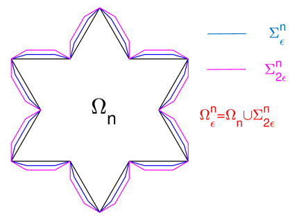
Figure 1: The domain $\Omega_{\varepsilon}^{n}$.

We can define, in a natural way, a finite Borel measure $\mu$ supported on $K$ by

$$\mu:=\mu_{1}+\mu_{2}+\mu_{3},$$ (1.3)

where $\mu_{i}$ denotes the normalized $d_{f}$-dimensional Hausdorff measure restricted to $K^{i}$, $i=1,2,3$, where $d_{f}=\frac{\log 4}{\log 3}$ is the Hausdorff measure of $K$.
For the measure $\mu$ there exist two positive constants $c_{1}$ and $c_{2}$ such that

$$c_{1}\,r^{d}\leq\mu(B(P,r)\cap K)\leq c_{2}\,r^{d},\ \forall\,P\in K,$$ (1.4)

where $d=d_{f}$ and $B(P,r)$ denotes the Euclidean ball of center $P$ and radius $r$. Since $\mu$ is supported on $K$, we can write $\mu(B(P,r))$ in (1.4) in place of $\mu(B(P,r)\cap K)$. We note that, in the terminology of [JoWa], from (1.4) it follows that $K$ is a $d_{f}$-set and the measure $\mu$ is a $d_{f}$-measure.

By $L^{p}(\cdot)$ we denote the Lebesgue space with respect to the Lebesgue measure $\mathrm{d}\mathcal{L}_{2}$ on subsets of $\mathbb{R}^{2}$, which will be left to the context whenever that does not create ambiguity. By $L^{p}(K,\mu)$ we denote the Banach space of $p$-summable functions on $K$ with respect to the invariant measure $\mu$. By $\ell$ we denote the natural arc length coordinate on each edge of $K_{n}$ and we introduce the coordinates $x=x(\ell)$, $y=y(\ell)$, on every segment of $K_{n}$. By $\mathrm{d}\ell$ we denote the one–dimensional measure given by the arc length $\ell$.
Let $\mathcal{G}$ be an open set of $\mathbb{R}^{2}$. By $W^{s,p}(\mathcal{G})$, where $s\in\mathbb{R}^{+}$, we denote the (possibly fractional) Sobolev spaces (see [necas]). Given $\mathcal{S}$ a closed set of $\mathbb{R}^{2}$, by $C^{0,\alpha}(\mathcal{S})$ we denote the space of Hölder continuous functions on $\mathcal{S}$ of exponent $\alpha$.

The domains $\Omega_{n}$ are $(\epsilon,\delta)$ domains with parameters $\epsilon$ and $\delta$ independent of the (increasing) number of sides of $K_{n}$ (see Lemma 3.3 in [capCPAA]). Thus, by the extension theorem for $(\epsilon,\delta)$ domains due to Jones (Theorem 1 in [Jones]), we obtain the following theorem, which provides an extension operator from $W^{1,p}(\Omega_{n})$ to the space ${W^{1,p}(\mathbb{R}^{2})}$ whose norm is independent of $n$ (see Theorem 5.7 in [capJMAA]).

Theorem 1.1.

There exists a bounded linear extension operator ${\hbox{\rm Ext}}_{J}:\,W^{1,p}(\Omega_{n})\to\,W^{1,p}(\mathbb{R}^{2})$ such that

$$\|{\hbox{\rm Ext}}_{J}\,v\|^{p}_{W^{1,p}(\mathbb{R}^{2})}\leq C_{J}\|v\|^{p}_{W^{1,p}(\Omega_{n})}$$ (1.5)

with $C_{J}$ independent of $n$.

We recall a Green formula for Lipschitz domains (see [bregil] and [baiocap]). Let $\mathcal{D}$ be a Lipschitz domain and let $(L^{p^{\prime}}_{\operatorname{div}}(\mathcal{D}))^{2}:=\{w\in(L^{p^{\prime}}(\mathcal{D}))^{2}\,:\,\operatorname{div}w\in L^{p^{\prime}}(\mathcal{D})\}$. Then, for every $u,v\in W^{1,p}(\mathcal{D})$ such that $w:=|\nabla{u}|^{p-2}\nabla u\in(L^{p^{\prime}}_{\operatorname{div}}(\mathcal{D}))^{2}$, since $\Delta_{p}u=\operatorname{div}(|\nabla u|^{p-2}\nabla u)$, it holds

$$\int_{\mathcal{D}}|\nabla u|^{p-2}\nabla u\nabla v\,\mathrm{d}\mathcal{L}_{2}=\left\langle\frac{\partial u}{\partial\nu}|\nabla u|^{p-2},v\right\rangle_{{}_{W^{-\frac{1}{p^{\prime}},p^{\prime}}(\partial\mathcal{D}),W^{\frac{1}{p^{\prime}},p}(\partial\mathcal{D})}}-\int_{\mathcal{D}}\Delta_{p}u\,v\,\mathrm{d}\mathcal{L}_{2}.$$

We now introduce Besov spaces on the fractal set $K$. From now on, we set $\alpha=1-\frac{2-d_{f}}{p}$. We define the Besov space on $K$ only for this particular $\alpha$, which is the case of our interest. For a general treatment, see [JoWa].