Channel-wise Topology Refinement Graph Convolution for Skeleton-Based Action Recognition

Abstract

Graph convolutional networks (GCNs) have been widely used and achieved remarkable results in skeleton-based action recognition. In GCNs, graph topology dominates feature aggregation and therefore is the key to extracting representative features. In this work, we propose a novel Channel-wise Topology Refinement Graph Convolution (CTR-GC) to dynamically learn different topologies and effectively aggregate joint features in different channels for skeleton-based action recognition. The proposed CTR-GC models channel-wise topologies through learning a shared topology as a generic prior for all channels and refining it with channel-specific correlations for each channel. Our refinement method introduces few extra parameters and significantly reduces the difficulty of modeling channel-wise topologies. Furthermore, via reformulating graph convolutions into a unified form, we find that CTR-GC relaxes strict constraints of graph convolutions, leading to stronger representation capability. Combining CTR-GC with temporal modeling modules, we develop a powerful graph convolutional network named CTR-GCN which notably outperforms state-of-the-art methods on the NTU RGB+D, NTU RGB+D 120, and NW-UCLA datasets.

1 Introduction

Human action recognition is an important task with various applications ranging from human-robot interaction to video surveillance. In recent years, skeleton-based human action recognition has attracted much attention due to the development of depth sensors and its robustness against complicated backgrounds.

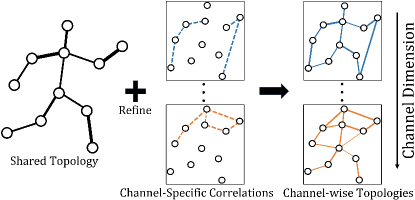
Figure 1: Channel-wise topology refinement. Lines of different colors correspond to topologies in different channels and the thickness of lines indicates the correlation strength between joints.

Early deep-learning-based methods treat human joints as a set of independent features and organize them into a feature sequence or a pseudo-image, which is fed into RNNs or CNNs to predict action labels. However, these methods overlook inherent correlations between joints, which reveals human body topology and is important information of human skeleton. Yan et al. [32] firstly modeled correlations between human joints with graphs and apply GCNs along with temporal convolutions to extract motion features. While the manually defined topology they employ is difficult to achieve relationship modeling between unnaturally connected joints and limits representation capability of GCNs. In order to boost power of GCNs, recent approaches [24, 35, 34] adaptively learn the topology of human skeleton through attention or other mechanisms. They use a topology for all channels, which forces GCNs to aggregate features with the same topology in different channels and thus limits the flexibility of feature extraction. Since different channels represent different types of motion features and correlations between joints under different motion features are not always the same, it’s not optimal to use one shared topology. Cheng et al. [3] set individual parameterized topologies for channel groups. However, the topologies of different groups are learned independently and the model becomes too heavy when setting channel-wise parameterized topologies, which increases the difficulty of optimization and hinders effective modeling of channel-wise topologies. Moreover, parameterized topologies remain the same for all samples, which is unable to model sample-dependent correlations.

In this paper, we propose a channel-wise topology refinement graph convolution which models channel-wise topology dynamically and effectively. Instead of learning topologies of different channels independently, CTR-GC learns channel-wise topologies in a refinement way. Specifically, CTR-GC learns a shared topology and channel-specific correlations simultaneously. The shared topology is a parameterized adjacency matrix that serves as topological priors for all channels and provides generic correlations between vertices. The channel-specific correlations are dynamically inferred for each sample and they capture subtle relationships between vertices within each channel. By refining the shared topology with channel-specific correlations, CTR-GC obtains channel-wise topologies (illustrated in Figure 1). Our refinement method avoids modeling the topology of each channel independently and introduces few extra parameters, which significantly reduces the difficulty of modeling channel-wise topologies. Moreover, through reformulating four categories of graph convolutions into a unified form, we verify the proposed CTR-GC essentially relaxes strict constraints of other categories of graph convolutions and improves the representation capability.

Combining CTR-GC with temporal modeling modules, we construct a powerful graph convolutional network named CTR-GCN for skeleton-based action recognition. Extensive experimental results on NTU RGB+D, NTU RGB+D 120, and NW-UCLA show that (1) our CTR-GC significantly outperforms other graph convolutions proposed for skeleton-based action recognition with comparable parameters and computation cost; (2) Our CTR-GCN exceeds state-of-the-art methods notably on all three datasets.

Our contributions are summarized as follows:

• We propose a channel-wise topology refinement graph convolution which dynamically models channel-wise topologies in a refinement approach, leading to flexible and effective correlation modeling.

• We mathematically unify the form of existing graph convolutions in skeleton-based action recognition and find that CTR-GC relaxes constraints of other graph convolutions, providing more powerful graph modeling capability.

• The extensive experimental results highlight the benefits of channel-wise topology and the refinement method. The proposed CTR-GCN outperforms state-of-the-art methods significantly on three skeleton-based action recognition benchmarks.

2 Related Work

2.1 Graph Convolutional Networks

Convolutional Neural Networks (CNNs) have achieved remarkable results in processing Euclidean data like images. To process non-Euclidean data like graphs, there is an increasing interest in developing Graph Convolutional Networks (GCNs). GCNs are often categorized as spectral methods and spatial methods. Spectral methods conduct convolution on spectral domain [1, 5, 11]. However, they depend on the Laplacian eigenbasis which is related to graph structure and thus can only be applied to graphs with same structure. Spatial methods define convolutions directly on the graph [7, 21, 29]. One of the challenges of spatial methods is to handle different sized neighborhoods. Among different GCN variants, the GCN proposed by Kipf et al. [11] is widely adapted to various tasks due to its simplicity. The feature update rule in [11] consists of two steps: (1) Transform features into high-level representations; and (2) Aggregate features according to graph topology. Our work adopts the same feature update rule.

2.2 GCN-based Skeleton Action Recognition

GCNs have been successfully adopted to skeleton-based action recognition [20, 24, 32, 34, 36, 27] and most of them follow the feature update rule of [11]. Due to the importance of topology (namely vertex connection relationship) in GCN, many GCN-based methods focus on topology modeling. According to the difference of topology, GCN-based methods can be categorized as follows: (1) According to whether the topology is dynamically adjusted during inference, GCN-based methods can be classified into static methods and dynamic methods. (2) According to whether the topology is shared across different channels, GCN-based methods can be classified into topology-shared methods and topology-non-shared methods.

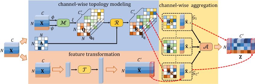
Figure 2: Framework of the proposed channel-wise topology refinement graph convolution. The channel-wise topology modeling refines the trainable shared topology with inferred channel-specific correlations. The feature transformation aims at transforming input features into high-level representations. Eventually, the output feature is obtained by channel-wise aggregation.

Static / Dynamic Methods. For static methods, the topologies of GCNs keep fixed during inference. Yan et al. [32] proposed an ST-GCN which predefines topology according to human body structure and the topology is fixed in both training and testing phase. Liu et al. [20] and Huang et al. [9] introduced multi-scale graph topologies to GCNs to enable multi-range joint relationship modeling. For dynamic methods, the topologies of GCNs are dynamically inferred during inference. Li et al. [15] proposed an A-links inference module to capture action-specific correlations. Shi et al. [24] and Zhang et al. [35] enhanced topology learning with self-attention mechanism, which models correlation between two joints given corresponding features. These methods infer correlations between two joints with local features. Ye et al. [34] proposed a Dynamic GCN, where contextual features of all joints are incorporated to learn correlations between any pairs of joints. Compared with static methods, dynamic methods have stronger generalization ability due to dynamic topologies.

Topology-shared / Topology-non-shared Methods. For topology-shared methods, the static or dynamic topologies are shared in all channels. These methods force GCNs to aggregate features in different channels with the same topology, limiting the upper bound of model performance. Most GCN-based methods follow topology-shared manner, including aforementioned static methods [9, 20, 32] and dynamic methods [15, 24, 34, 35]. Topology-non-shared methods use different topologies in different channels or channel groups, which naturally overcome limitations of topology-shared methods. Cheng et al. [3] proposed a DC-GCN which sets individual parameterized topologies for different channel groups. However, the DC-GCN faces difficulty of optimization caused by excessive parameters when setting channel-wise topologies. To our best knowledge, topology-non-shared graph convolutions are rarely explored in the skeleton-based action recognition, and this work is the first to model dynamic channel-wise topologies. Note that our method also belongs to dynamic methods because topologies are dynamically inferred during inference.

3 Method

In this section, we first define related notations and formulate conventional graph convolution. Then we elaborate our Channel-wise Topology Refinement Graph Convolution (CTR-GC) and mathematically analyze the representation capability of CTR-GC and other graph convolutions. Finally, we introduce the structure of our CTR-GCN.

3.1 Preliminaries

Notations. A human skeleton is represented as a graph with joints as vertices and bones as edges. The graph is denoted as $\mathcal{G=(V,E,X)}$, where $\mathcal{V}=\{v_{1},v_{2},......,v_{N}\}$ is the set of $N$ vertices. $\mathcal{E}$ is the edge set, which is formulated as an adjacency matrix $\mathbf{A}\in\mathbb{R}^{N\times N}$ and its element $a_{ij}$ reflects the correlation strength between $v_{i}$ and $v_{j}$. The neighborhood of $v_{i}$ is represented as $\mathcal{N}(v_{i})=\{v_{j}|a_{ij}\neq 0\}$. $\mathcal{X}$ is the feature set of $N$ vertices, which is represented as a matrix $\mathbf{X}\in\mathbb{R}^{N\times C}$ and $v_{i}$’s feature is represented as $\mathbf{x_{i}}\in\mathbb{R}^{C}$.

Topology-shared Graph Convolution. The normal topology-shared graph convolution utilizes the weight $\mathbf{W}$ for feature transformation and aggregate representations of $v_{i}$’s neighbor vertices through $a_{ij}$ to update its representation $\mathbf{z_{i}}$, which is formulated as

$$\vspace{-0.2cm}\mathbf{z_{i}}=\sum_{v_{j}\in\mathcal{N}(v_{i})}a_{ij}\mathbf{x_{j}}\mathbf{W}$$ (1)

For static methods, $a_{ij}$ is defined manually or set as trainable parameter. For dynamic methods, $a_{ij}$ is usually generated by the model depending on the input sample.

3.2 Channel-wise Topology Refinement Graph Convolution

The general framework of our CTR-GC is shown in Figure 2. We first transform input features into high-level features, then dynamically infer channel-wise topologies to capture pairwise correlations between input sample’s joints under different types of motion features, and aggregate features in each channel with corresponding topology to get the final output. Specifically, our CTR-GC contains three parts: (1) Feature transformation which is done by transformation function $\mathcal{T}(\cdot)$; (2) Channel-wise topology modeling which consists of correlation modeling function $\mathcal{M}(\cdot)$ and refinement function $\mathcal{R}(\cdot)$; (3) Channel-wise aggregation which is completed by aggregation function $\mathcal{A}(\cdot)$. Given the input feature $\mathbf{X}\in\mathbb{R}^{N\times C}$, the output $\mathbf{Z}\in\mathbb{R}^{N\times C^{\prime}}$ of CTR-GC is formulated as

$$\vspace{-0.1cm}\mathbf{Z}=\mathcal{A}\big{(}\mathcal{T}(\mathbf{X}),\mathcal{R}(\mathcal{M}(\mathbf{X}),\mathbf{A})\big{)},$$ (2)

where $\mathbf{A}\in\mathbb{R}^{N\times N}$ is the learnable shared topology. Next, we introduce these three parts in detailed.

Feature Transformation. As shown in the orange block in Figure 2, feature transformation aims at transforming input features into high-level representations via $\mathcal{T}(\cdot)$. We adopt a simple linear transformation here as the topology-shared graph convolution, which is formulated as

$$\vspace{-0.3cm}\mathbf{\widetilde{X}}=\mathcal{T}(\mathbf{X})=\mathbf{XW},$$ (3)

where $\mathbf{\widetilde{X}}\in\mathbb{R}^{N\times C^{\prime}}$ is the transformed feature and $\mathbf{W}\in\mathbb{R}^{C\times C^{\prime}}$ is the weight matrix. Note that other transformations can also be used, e.g., multi-layer perceptron.

Channel-wise Topology Modeling. The channel-wise topology modeling is shown in the blue block in Figure 2. The adjacency matrix is used as shared topology for all channels and is learned through backpropagation. Moreover, we learn channel-specific correlations $\mathbf{Q}\in\mathbb{R}^{N\times N\times C^{\prime}}$ to model specific relationships between vertices in $C^{\prime}$ channels. Then the channel-wise topologies $\mathbf{R}\in\mathbb{R}^{N\times N\times C^{\prime}}$ are obtained by refining the shared topology $\mathbf{A}$ with $\mathbf{Q}$.

Specifically, we first employ correlation modeling function $\mathcal{M}(\cdot)$ to model channel-wise correlations between vertices. To reduce computation cost, we utilize linear transformations $\phi$ and $\psi$ to reduce feature dimension before sending input features into $\mathcal{M}(\cdot)$. Given a pair of vertices $(v_{i},v_{j})$ and their corresponding features $(\mathbf{x_{i}},\mathbf{x_{j}})$, we design two simple yet effective correlation modeling functions. The first correlation modeling function $\mathcal{M}_{1}(\cdot)$ is formulated as

$$\vspace{-0.16cm}\mathcal{M}_{1}(\psi(\mathbf{x_{i}}),\phi(\mathbf{x_{j}}))=\sigma(\psi(\mathbf{x_{i}})-\phi(\mathbf{x_{j}})),$$ (4)

where $\sigma(\cdot)$ is activation function. $\mathcal{M}_{1}(\cdot)$ essentially calculates distances between $\psi(\mathbf{x_{i}})$ and $\phi(\mathbf{x_{j}})$ along channel dimension and utilizes the nonlinear transformations of these distances as channel-specific topological relationship between $v_{i}$ and $v_{j}$. The second correlation modeling function $\mathcal{M}_{2}(\cdot)$ is formulated as

$$\vspace{-0.16cm}\mathcal{M}_{2}(\psi(\mathbf{x_{i}}),\phi(\mathbf{x_{j}}))=MLP(\psi(\mathbf{x_{i}})||\phi(\mathbf{x_{j}})),$$ (5)

where $||$ is concatenate operation and MLP is multi-layer perceptron. We utilize MLP here due to its powerful fitting capability.

Based on the correlation modeling function, the channel-specific correlations $\mathbf{Q}\in\mathbb{R}^{N\times N\times C^{\prime}}$ are obtained by employing linear transformation $\xi$ to raise the channel dimension, which is formulated as

$$\vspace{-0.16cm}\mathbf{q_{ij}}=\xi\Big{(}\mathcal{M}\big{(}\psi(\mathbf{x_{i}}),\phi(\mathbf{x_{j}})\big{)}\Big{)},\ i,j\in\{1,2,\cdots,N\},$$ (6)

where $\mathbf{q_{ij}}\in\mathbb{R}^{C^{\prime}}$ is a vector in $\mathbf{Q}$ and reflects the channel-specific topological relationship between $v_{i}$ and $v_{j}$. Note that $\mathbf{Q}$ is not forced to be symmetric, i.e., $\mathbf{q_{ij}}\neq\mathbf{q_{ji}}$, which increases the flexibility of correlation modeling.

Eventually, the channel-wise topologies $\mathbf{R}\in\mathbb{R}^{N\times N\times C^{\prime}}$ are obtained by refining the shared topology $\mathbf{A}$ with channel-specific correlations $\mathbf{Q}$:

$$\vspace{-0.16cm}\mathbf{R}=\mathcal{R}(\mathbf{Q},\mathbf{A})=\mathbf{A}+\alpha\cdot\mathbf{Q},$$ (7)

where $\alpha$ is a trainable scalar to adjust the intensity of refinement. The addition is conducted in a broadcast way where $\mathbf{A}$ is added to each channel of $\alpha\times\mathbf{Q}$.

Channel-wise Aggregation. Given the refined channel-wise topologies $\mathbf{R}$ and high-level features $\mathbf{\widetilde{X}}$, CTR-GC aggregates features in a channel-wise manner. Specifically, CTR-GC constructs a channel-graph for each channel with corresponding refined topology $\mathbf{R_{c}}\in\mathbb{R}^{N\times N}$ and feature $\mathbf{\tilde{x}_{:,c}}\in\mathbb{R}^{N\times 1}$, where $\mathbf{R_{c}}$ and $\mathbf{\tilde{x}_{:,c}}$ are respectively from $\mathbf{c}$-th channel of $\mathbf{R_{c}}$ and $\mathbf{\widetilde{X}}$ ($c\in\{1,\cdots,C^{\prime}\}$). Each channel-graph reflects relationships of vertices under a certain type of motion feature. Consequently, feature aggregation is performed on each channel-graph, and the final output $\mathbf{Z}$ is obtained by concatenating the output features of all channel-graphs, which is formulated as

$$\vspace{-0.15cm}\mathbf{Z}=\mathcal{A}(\mathbf{\widetilde{X},R})=[\mathbf{R_{1}}\mathbf{\tilde{x}_{:,1}}||\mathbf{R_{2}}\mathbf{\tilde{x}_{:,2}}||\cdots||\mathbf{R_{C^{\prime}}}\mathbf{\tilde{x}_{:,C^{\prime}}}],$$ (8)

where $||$ is concatenate operation. During the whole process, the inference of channel-specific correlations $\mathbf{Q}$ relies on input samples as shown in Equation 6. Therefore, the proposed CTR-GC is a dynamic graph convolution and it adaptively varies with different input samples.

3.3 Analysis of Graph Convolutions

We analyze the representation capability of different graph convolutions by reformulating them into a unified form and comparing them with dynamic convolution [2, 33] employed in CNNs.

We first recall dynamic convolution which enhances vanilla convolution with dynamic weights. In dynamic convolution, each neighbor pixel $p_{j}$ of the center pixel $p_{i}$ has a corresponding weight in the convolution kernel, and the weight can be dynamically adjusted according to different input samples, which makes the dynamic convolution have strong representation ability. The dynamic convolution can be formulated as

$$\vspace{-0.15cm}\mathbf{z_{i}^{k}}=\sum_{p_{j}\in\mathcal{N}(p_{i})}\mathbf{x_{j}^{k}}\mathbf{W_{j}^{k}},$$ (9)

where $\mathbf{k}$ indicates the index of input sample. $\mathbf{x_{j}^{k}}$ and $\mathbf{z_{i}^{k}}$ are the input feature of $p_{j}$ and the output feature of $p_{i}$ of the $\mathbf{k}$-th sample. $\mathbf{W_{j}^{k}}$ is the dynamic weight.

Due to the irregular structure of the graph, the correspondence between neighbor vertices and weights is difficult to establish. Thus, graph convolutions (GCs) degrade convolution weights into adjacency weights (i.e., topology) and weights shared in the neighborhood. However, sharing weights in the neighborhood limits representation capability of GCs. To analyze the gap of representation ability between different GCs and dynamic convolution, we integrate adjacency weights and weights shared in the neighborhood into a generalized weight matrix $\mathbf{E^{k}_{ij}}$. Namely, we formulate all GCs in the form of $\mathbf{z_{i}^{k}}=\sum_{v_{j}\in\mathcal{N}(v_{i})}\mathbf{x_{j}^{k}}\mathbf{E^{k}_{ij}}$ where $\mathbf{E^{k}_{ij}}$ is generalized weight. We classified GCs into four categories as mentioned before.

Static Topology-shared GCs. In static topology-shared GCs, the topologies keep fixed for different samples and are shared across all channels, which can be formulated as

$$\mathbf{z_{i}^{k}}=\sum_{v_{j}\in\mathcal{N}(v_{i})}a_{ij}\mathbf{x_{j}^{k}}\mathbf{W}=\sum_{v_{j}\in\mathcal{N}(v_{i})}\mathbf{x_{j}^{k}}(a_{ij}\mathbf{W}),$$ (10)

where $a_{ij}\mathbf{W}$ is the generalized weight of static topology-shared GC. From Equation 9 and 10, it can be seen that the difference between dynamic convolution and static topology-shared GC lies in their (generalized) weights. Specifically, the weights of dynamic convolution $\mathbf{W_{j}^{k}}$ is individual for each $j$ and $k$, while generalized weights of static topology-shared GC is subject to following constraints:

Constraint 1: $\mathbf{E^{k_{1}}_{ij}}$ and $\mathbf{E^{k_{2}}_{ij}}$ are forced to be same.

Constraint 2: $\mathbf{E^{k}_{ij_{1}}}$ and $\mathbf{E^{k}_{ij_{2}}}$ differ by a scaling factor.

Note that $\mathbf{k_{1}},\mathbf{k_{2}}$ are different sample indices and $\mathbf{j_{1}},\mathbf{j_{2}}$ are different neighbor vertex indices. These constraints cause the gap of representation ability between static topology-shared GCs and dynamic convolutions. Note that we concentrate on the neighborhood rooted at $v_{i}$ and do not consider the change of $v_{i}$ for simplicity.

Dynamic topology-shared GCs. Compared with static topology-shared GCs, the dynamic ones infer topologies dynamically and thus have better generalization ability. The formulation of dynamic topology-shared GCs is

$$\vspace{-0.15cm}\mathbf{z_{i}^{k}}=\sum_{v_{j}\in\mathcal{N}(v_{i})}a_{ij}^{k}\mathbf{x_{j}^{k}}\mathbf{W}\\ =\sum_{v_{j}\in\mathcal{N}(v_{i})}\mathbf{x_{j}^{k}}(a_{ij}^{k}\mathbf{W}),$$ (11)

where $a_{ij}^{k}$ is dynamic topological relationship between $v_{i}$, $v_{j}$ and depends on input sample. It can be seen that the generalized weights of dynamic topology-shared GCs still suffer from Constraint 2 but relax Constraint 1 into the following constraint:

Constraint 3: $\mathbf{E^{k_{1}}_{ij}}$, $\mathbf{E^{k_{2}}_{ij}}$ differ by a scaling factor.

Static topology-non-shared GCs. This kind of GCs utilize different topologies for different channels (groups). Here we just analyze static GCs with channel-wise topologies because it is the most generalized form of static topology-non-shared GCs and can degenerate into others, e.g., static group-wise-topology GCs. The specific formulation is

$$\mathbf{z_{i}^{k}} =\sum_{v_{j}\in\mathcal{N}(v_{i})}\mathbf{p_{ij}}\odot(\mathbf{x_{j}^{k}}\mathbf{W})$$ (12)

$$=\sum_{v_{j}\in\mathcal{N}(v_{i})}\mathbf{x_{j}^{k}}\big{(}[p_{ij1}\mathbf{w_{:,1}},\cdots,p_{ijC^{\prime}}\mathbf{w_{:,C^{\prime}}}]\big{)},\vspace{-0.5cm}$$ (13)

where $\odot$ is element-wise multiplication and $\mathbf{p_{ij}}\in\mathbb{R}^{C^{\prime}}$ is channel-wise topological relationship between $v_{i}$, $v_{j}$. $p_{ijc}$ is the $c$-th element of $\mathbf{p_{ij}}$. $\mathbf{w_{:,c}}$ is the $c$-th column of $\mathbf{W}$. (We omit the derivation of Equation 12 and 13 for clarity. The details can be found in the supplementary materials.) From Equation 13, we observe that generalized weights of this kind of GCs suffer from Constraint 1 due to static topology but relax Constraint 2 into the following constraint:

Constraint 4: Different corresponding columns of $\mathbf{E^{k}_{ij_{1}}}$ and $\mathbf{E^{k}_{ij_{2}}}$ differ by different scaling factors.

Dynamic topology-non-shared GCs. The only difference between static topology-non-shared GCs and dynamic topology-non-shared GCs is that dynamic topology-non-shared GCs infers non-shared topologies dynamically, thus dynamic topology-non-shared GCs can be formulated as

$$\vspace{-0.15cm}\mathbf{z_{i}^{k}}=\sum_{v_{j}\in\mathcal{N}(v_{i})}\mathbf{x_{j}^{k}}\big{(}[r_{ij1}^{k}\mathbf{w_{:,1}},\cdots,r_{ijC^{\prime}}^{k}\mathbf{w_{:,C^{\prime}}}]\big{)},$$ (14)

where $r_{ijc}^{k}$ is the $\mathbf{k}$-th sample’s dynamic topological relationship between $v_{i}$, $v_{j}$ in the $c$-th channel. Obviously, generalized weights of dynamic topology-non-shared graph convolution relax both Constraint 1 and 2. Specifically, it relaxes Constraint 2 into Constraint 4 and relaxes Constraint 1 into the following constraint:

Constraint 5: Different corresponding columns of $\mathbf{E^{k_{1}}_{ij}}$ and $\mathbf{E^{k_{2}}_{ij}}$ differ by different scaling factors.

Topology		Constraints					Instance
Non-shared	Dynamic	1	2	3	4	5
✗	✗	✓	✓				ST-GC[32]
✗	✓		✓	✓			AGC [24], Dy-GC[34]
✓	✗	✓			✓		DC-GC [3]
✓	✓				✓	✓	CTR-GC (ours)

Table 1: Constraints on different categories of graph convolutions and corresponding instances. The number 1-5 correspond to five constraints. Red, Green and Blue respectively indicate the relatively High, Mid and Low constraint strength.

We conclude different categories of graph convolutions and their constraints in Table 1. It can be seen that dynamic topology-non-shared GC is the least constrained. Our CTR-GC belongs to dynamic topology-non-shared GC and Equation 8 can be reformulated to Equation 14, indicating that theoretically CTR-GC has stronger representation capability than previous graph convolutions [3, 24, 32, 34]. The specific reformulation is shown in supplemental materials.

3.4 Model Architecture

Based on CTR-GC, we construct a powerful graph convolutional network CTR-GCN for skeleton-based action recognition. We set the neighborhood of each joint as the entire human skeleton graph, which is proved to be more effective in this task by previous work [4, 24]. The entire network consists of ten basic blocks, followed by a global average pooling and a softmax classifier to predict action labels. The number of channels for ten blocks are 64-64-64-64-128-128-128-256-256-256. Temporal dimension is halved at the 5-th and 8-th blocks by strided temporal convolution. The basic block of our CTR-GCN is shown in Figure 3 (a). Each block mainly consists of a spatial modeling module, a temporal modeling module and residual connections.

Spatial Modeling. In a spatial modeling module, we use three CTR-GCs in parallel to extract correlations between human joints and sum up their results as output. For clarity, an instance of CTR-GC with $\mathcal{M}_{1}(\cdot)$ is illustrated in Figure 3 (b). Our CTR-GC is designed to extract features of a graph with input feature $\mathbf{X}\in\mathbb{R}^{N\times C}$. To adopt CTR-GC to a skeleton graph sequence $\mathbf{S}\in\mathbb{R}^{T\times N\times C}$, we pool $\mathbf{S}$ along temporal dimension and use pooled features to infer channel-wise topologies. Specifically, CTR-GC first utilizes $\phi$ and $\psi$ with reduction rate $r$ to extract compact representations. Then temporal pooling is used to aggregate temporal features. After that, CTR-GC conducts pair-wise subtraction and activation following Equation 4. The channel dimension of activation is then raised with $\xi$ to obtain channel-specific correlations, which are used to refine the shared topology $\mathbf{A}$ to obtain channel-wise topologies. Eventually, channel-wise aggregation (implemented by batch matrix multiplication) is conducted in each skeleton graph to obtain the output representation $\mathbf{S^{o}}$.

Temporal Modeling. To model actions with different duration, we design a multi-scale temporal modeling module following [20]. The main difference is that we use fewer branches for that too many branches slow down inference speed. As shown in Figure 3 (a), this module contains four branches, each containing a $1\times 1$ convolution to reduce channel dimension. The first three branches contain two temporal convolutions with different dilations and one MaxPool respectively following $1\times 1$ convolution. The results of four branches are concatenated to obtain the output.

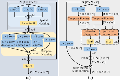
Figure 3: (a) The basic block of our CTR-GCN. (b)CTR-GC with correlation modeling function $\mathcal{M}_{1}(\cdot)$ or $\mathcal{M}_{2}(\cdot)$.

4 Experiments

4.1 Datasets

NTU RGB+D. NTU RGB+D [22] is a large-scale human action recognition dataset containing 56,880 skeleton action sequences. The action samples are performed by 40 volunteers and categorized into 60 classes. Each sample contains an action and is guaranteed to have at most 2 subjects, which is captured by three Microsoft Kinect v2 cameras from different views concurrently. The authors of this dataset recommend two benchmarks: (1) cross-subject (X-sub): training data comes from 20 subjects, and testing data comes from the other 20 subjects. (2) cross-view (X-view): training data comes from camera views 2 and 3, and testing data comes from camera view 1.

NTU RGB+D 120. NTU RGB+D 120 [17] is currently the largest dataset with 3D joints annotations for human action recognition, which extends NTU RGB+D with additional 57,367 skeleton sequences over 60 extra action classes. Totally 113,945 samples over 120 classes are performed by 106 volunteers, captured with three cameras views. This dataset contains 32 setups, each denoting a specific location and background. The authors of this dataset recommend two benchmarks: (1) cross-subject (X-sub): training data comes from 53 subjects, and testing data comes from the other 53 subjects. (2) cross-setup (X-setup): training data comes from samples with even setup IDs, and testing data comes from samples with odd setup IDs.

Northwestern-UCLA. Northwestern-UCLA dataset [31] is captured by three Kinect cameras simultaneously from multiple viewpoints. It contains 1494 video clips covering 10 action categories. Each action is performed by 10 different subjects. We follow the same evaluation protocol in [31]: training data from the first two cameras, and testing data from the other camera.

4.2 Implementation Details

All experiments are conducted on one RTX 2080 TI GPU with the PyTorch deep learning framework. Our models are trained with SGD with momentum 0.9, weight decay 0.0004. The training epoch is set to 65 and a warmup strategy [8] is used in the first 5 epochs to make the training procedure more stable. Learning rate is set to 0.1 and decays with a factor 0.1 at epoch 35 and 55. For NTU RGB+D and NTU RGB+D 120, the batch size is 64, each sample is resized to 64 frames, and we adopt the data pre-processing in [35]. For Northwestern-UCLA, the batch size is 16, and we adopt the data pre-processing in [4].

4.3 Ablation Study

In this section, we analyze the proposed channel-wise topology refinement graph convolution and its configuration on the X-sub benchmark of the NTU RGB+D 120 dataset.

Effectiveness of CTR-GC.

Methods	Param.	Acc (%)
Baseline	1.22M	83.4
+2 CTR-GC	1.26M	84.2 ↑0.8
+5 CTR-GC	1.35M	84.7 ↑1.3
CTR-GCN w/o Q	1.22M	83.7 ↑0.3
CTR-GCN w/o A	1.46M	84.0 ↑0.6
CTR-GCN	1.46M	84.9 ↑1.5

Table 2: Comparisons of accuracies when adding CTR-GCs gradually and removing A or Q from CTR-GCN.

We employ ST-GCN [32] as the baseline, which belongs to static topology-shared graph convolution and the topology is untrainable. We further add residual connections in ST-GCN as our basic block and replace its temporal convolution with temporal modeling module described in Section 3.4 for fair comparison.

The experimental results are shown in Table 2. First, we gradually replace GCs with CTR-GCs (shown in Figure 3 (b) and $r=8$) in the baseline. We observe that accuracies increase steadily and the accuracy is substantially improved when all GCs are replaced by CTR-GCs (CTR-GCN), which validates the effectiveness of CTR-GC.

Then we validate effects of the shared topology A and the channel-specific correlations Q respectively by removing either of them from CTR-GCN. CTR-GCN w/o Q shares a trainable topology across different channels. We observe that its performance drops 1.2% compared with CTR-GCN, indicating the importance of modeling channel-wise topologies. The performance of CTR-GCN w/o A drops 0.9%, confirming that it’s hard to model individual topology for each channel directly and topology refinement provides an effective approach to solve this problem.

Configuration Exploration.

Methods	$\boldsymbol{\mathcal{M}}$	$\boldsymbol{r}$	$\boldsymbol{\sigma}$	Param.	Acc (%)
Baseline	-	-	-	1.21M	83.4
A	$\mathcal{M}_{1}^{+}$	8	Tanh	1.46M	84.9↑1.5
B	$\mathcal{M}_{1}$	8	Tanh	1.46M	84.9↑1.5
C	$\mathcal{M}_{2}$	8	Tanh	1.48M	84.8↑1.4
D	$\mathcal{M}_{1}$	4	Tanh	1.69M	84.8↑1.4
E	$\mathcal{M}_{1}$	16	Tanh	1.34M	84.5↑1.1
F	$\mathcal{M}_{1}$	8	Sig	1.46M	84.6↑1.2
G	$\mathcal{M}_{1}$	8	ReLU	1.46M	84.8↑1.4

Table 3: Comparisons of the validation accuracy of CTR-GC with different settings.

We explore different configurations of CTR-GC, including the choice of correlation modeling functions $\mathcal{M}$, the reduction rate $r$ of $\phi$ and $\psi$, activation function $\sigma$ of correlation modeling function. As shown in Table 3, we observe that models under all configurations outperform the baseline, confirming the robustness of CTR-GC. (1) Comparing models A, B and C, we find models with different correlation modeling functions all achieve good performance, which indicates that channel-wise topology refinement is a generic idea and is compatible with many different correlation modeling functions ($\mathcal{M}_{1}^{+}$ replaces the subtraction in $\mathcal{M}_{1}$ with addition). (2) Comparing models B, D and E, we find models with $r=4,8$ (models B, D) achieve better results and the model with $r=8$ (model B) performs better slightly with fewer parameters. Model E with $r=16$ performs worse because too few channels are used in correlation modeling function, which is not sufficient to effectively model channel-specific correlations. (3) Comparing models B, F and G, Sigmoid and ReLU perform worse than Tanh and we argue that non-negative output values of Sigmoid and ReLU constrains the flexibility of correlation modeling. Considering performance and efficiency, we choose model B as our final model.

4.4 Comparison with Other GCs

Topology		Methods	Param.	FLOPs	Acc (%)
Non-share	Dynamic
✗	✗	ST-GC [32]	1.22M	~1.65G	83.4
✗	✓	AGC [24]	1.55M	~2.11G	83.9
✗	✓	Dy-GC [34]	1.73M	~1.66G	83.9
✓	✗	DC-GC [3]	1.51M	~1.65G	84.2
✓	✗	DC-GC*[3]	3.37M	~1.65G	84.0
✓	✓	CTR-GC	1.46M	~1.97G	84.9

Table 4: Comparisons of CTR-GC with other graph convolutions. The first two columns show the categories of graph convolutions.

In order to validate the effectiveness of our CTR-GC, we compare performance, parameters and computation cost of CTR-GC against other graph convolutions in Table 4. Specifically, we keep the backbone of the baseline model and only replace graph convolutions for fair comparison. Note that DC-GC split channels into 16 groups and set a trainable adjacency matrix for each group, while DC-GC* set a trainable adjacency matrix for each channel. From Table 4, we observe that (1) On the whole, topology-non-shared methods achieve better performance than topology-shared methods, and dynamic methods perform better than static methods, indicating the importance of modeling non-shared topologies and dynamic topologies; (2) Compared with DC-GC, DC-GC* performs worse while has much more parameters, confirming that it’s not effective to model channel-wise topologies with parameterized adjacency matrices alone; (3) CTR-GC outperforms DC-GC* by 0.9%, proving that our refinement approach is effective to model channel-wise topologies. Moreover, our CTR-GC introduces little extra parameters and computation cost compared with other graph convolutions.

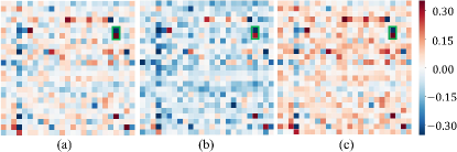
Figure 4: (a) The shared topology. (b) and (c) The refined channel-wise topologies of different channels.

4.5 Visualization of Learned Topologies

We illustrate the shared topology and refined channel-wise topologies of an action sample “typing on the keyboard” in Figure 4. The values close to 0 indicate weak relationships between joints and vice versa. We observe that (1) the shared topology is different from refined channel-wise topologies, indicating that our method can effectively refine the shared topology. (2) the refined channel-wise topologies are different, demonstrating that our method can learn individual topologies depending on specific motion features for different channels. (3) Some correlations are consistently strong in all channels, indicating that these joint pairs are strongly relevant in general, e.g., the correlation between left elbow and left-hand tip (blue square in the green box), and the correlation between left-hand tip and left wrist (red square in the green box). It’s reasonable for “typing on the keyboard” where main motion happens on hands.

4.6 Comparison with the State-of-the-Art

Methods	NTU-RGB+D 120
	X-Sub (%)	X-Set (%)
ST-LSTM[18]	55.7	57.9
GCA-LSTM[19]	61.2	63.3
RotClips+MTCNN[10]	62.2	61.8
SGN[35]	79.2	81.5
2s-AGCN[24]	82.9	84.9
Shift-GCN[4]	85.9	87.6
DC-GCN+ADG[3]	86.5	88.1
MS-G3D[20]	86.9	88.4
PA-ResGCN-B19 [26]	87.3	88.3
Dynamic GCN [34]	87.3	88.6
CTR-GCN (Bone Only)	85.7	87.5
CTR-GCN (Joint+Bone)	88.7	90.1
CTR-GCN	88.9	90.6

Table 5: Classification accuracy comparison against state-of-the-art methods on the NTU RGB+D 120 dataset.

Methods	NTU-RGB+D
	X-Sub (%)	X-View (%)
Ind-RNN[16]	81.8	88.0
HCN[14]	86.5	91.1
ST-GCN[32]	81.5	88.3
2s-AGCN[24]	88.5	95.1
SGN[35]	89.0	94.5
AGC-LSTM[25]	89.2	95.0
DGNN[23]	89.9	96.1
Shift-GCN[4]	90.7	96.5
DC-GCN+ADG[3]	90.8	96.6
PA-ResGCN-B19 [26]	90.9	96.0
DDGCN[12]	91.1	97.1
Dynamic GCN[34]	91.5	96.0
MS-G3D[20]	91.5	96.2
CTR-GCN	92.4	96.8

Table 6: Classification accuracy comparison against state-of-the-art methods on the NTU RGB+D dataset.

Methods	Northwestern-UCLA
	Top-1 (%)
Lie Group[28]	74.2
Actionlet ensemble[30]	76.0
HBRNN-L[6]	78.5
Ensemble TS-LSTM[13]	89.2
AGC-LSTM[25]	93.3
Shift-GCN[4]	94.6
DC-GCN+ADG[3]	95.3
CTR-GCN	96.5

Table 7: Classification accuracy comparison against state-of-the-art methods on the Northwestern-UCLA dataset.

Many state-of-the-art methods employ a multi-stream fusion framework. We adopt same framework as [4, 34] for fair comparison. Specifically, we fuse results of four modalities, i.e., joint, bone, joint motion, and bone motion.

We compare our models with the state-of-the-art methods on NTU RGB+D 120, NTU RGB+D and NW-UCLA in Tables 5, 6 and 7 respectively. On three datasets, our method outperforms all existing methods under nearly all evaluation benchmarks. On NTU-RGB+D 120, our model with joint-bone fusion achieves state-of-the-art performance, and our CTR-GCN outperforms current state-of-the-art Dynamic GCN [34] by 1.6% and 2.0% on the two benchmarks respectively. Notably, our method is the first to model channel-wise topologies dynamically which is very effective in skeleton-based action recognition.

5 Conclusion

In this work, we present a novel channel-wise topology refinement graph convolution (CTR-GC) for skeleton-based action recognition. CTR-GC learns channel-wise topologies in a refinement way which shows powerful correlation modeling capability. Both mathematical analysis and experimental results demonstrate that CTR-GC has stronger representation capability than other graph convolutions. On three datasets, the proposed CTR-GCN outperforms state-of-the-art methods.

Acknowledgment This work is supported by the National Key R&D Plan (No.2018YFC0823003), Beijing Natural Science Foundation (No.L182058), the Natural Science Foundation of China (No.61972397,62036011,61721004), the Key Research Program of Frontier Sciences, CAS (No.QYZDJ-SSW-JSC040), National Natural Science Foundation of China (No.U2033210).

Supplemental Materials for Channel-wise Topology Refinement Graph Convolution for Skeleton-Based Action Recognition

This supplemental materials include details about formula derivation, architecture setting, more visualizations and other ablation studies. Specifically, we give the derivation from Equation 12 to 13 and from Equation 8 to 14. Then we show the detailed architecture of CTR-GCN, including input size, output size and specific hyperparameters of each block. Moreover, we visualize shared topologies and channel-specific correlations. At last, we conduct ablation studies on the effect of CTR-GC’s number per block, temporal convolution, and analyze the performance of different graph convolutions on hard classes.

Formula Derivation

We first give the derivation from Equation 12 to 13. The Equation 12 is

$$\vspace{-0.16cm}\mathbf{z^{k}_{i}}=\sum_{v_{j}\in\mathcal{N}(v_{i})}\mathbf{p_{ij}}\odot(\mathbf{x^{k}_{j}W}),$$ (15)

where $\mathbf{z^{k}_{i}}\in\mathbb{R}^{1\times C^{\prime}}$ is the output feature of $v_{i}$ and $\mathbf{p_{ij}}\in\mathbb{R}^{1\times C^{\prime}}$ is the channel-wise relationship between $v_{i}$ and $v_{j}$. $\mathbf{x^{k}_{j}}\in\mathbb{R}^{1\times C}$ is the input feature of $v_{j}$ and $\mathbf{W}\in\mathbb{R}^{C\times C^{\prime}}$ is weight matrix. The $c$-th element of $\mathbf{z^{k}_{i}}$ is formulated as

$$z^{k}_{ic} =\sum_{v_{j}\in\mathcal{N}(v_{i})}p_{ijc}\mathbf{(x^{k}_{j}W)_{c}}=\sum_{v_{j}\in\mathcal{N}(v_{i})}p_{ijc}\mathbf{(x^{k}_{j}w_{:,c})}$$

$$=\sum_{v_{j}\in\mathcal{N}(v_{i})}\mathbf{x^{k}_{j}}(p_{ijc}\mathbf{w_{:,c}}),\vspace{-0.16cm}$$ (16)

where $p_{ijc}$ is the $c$-th element of $\mathbf{p_{ij}}$. $\mathbf{(x^{k}_{j}W)_{c}}\in\mathbb{R}^{1}$ is the $c$-th element of $\mathbf{x^{k}_{j}W}$ and $\mathbf{w_{:,c}}\in\mathbb{R}^{C\times 1}$ is the $c$-th column of $\mathbf{W}$. Therefore, $\mathbf{z^{k}_{i}}$ can be formulated as

$$\mathbf{z^{k}_{i}} =\left[\begin{array}[]{c}\sum_{v_{j}\in\mathcal{N}(v_{i})}\mathbf{x^{k}_{j}}(p_{ij1}\mathbf{w_{:,1}})\\ \vdots\\ \sum_{v_{j}\in\mathcal{N}(v_{i})}\mathbf{x^{k}_{j}}(p_{ijC^{\prime}}\mathbf{w_{:,C^{\prime}}})\end{array}\right]^{T}$$ (20)

$$=\sum_{v_{j}\in\mathcal{N}(v_{i})}\mathbf{x^{k}_{j}}([p_{ij1}\mathbf{w_{:,1}},\cdots,p_{ijC^{\prime}}\mathbf{w_{:,C^{\prime}}}]),$$ (21)

which is the same as Equation 13.

Then we give the derivation from Equation 8 to 14. We add sample index $\mathbf{k}$ in Equation 8, which is formulated as

$$\vspace{-0.16cm}\mathbf{Z^{k}}=[\mathbf{R^{k}_{1}\tilde{x}^{k}_{:,1}}||\mathbf{R^{k}_{2}\tilde{x}^{k}_{:,2}}||\cdots||\mathbf{R^{k}_{C^{\prime}}\tilde{x}^{k}_{:,C^{\prime}}}].$$ (22)

The $c$-th column of $\mathbf{Z^{k}}\in\mathbb{R}^{N\times C^{\prime}}$ can be formulated as

$$\vspace{-0.16cm}\mathbf{z^{k}_{:,c}}=\mathbf{R^{k}_{c}\tilde{x}^{k}_{:,c}}=\mathbf{R^{k}_{c}}\mathbf{(X^{k}W)_{:,c}}=\mathbf{R^{k}_{c}}\mathbf{(X^{k}w_{:,c})},$$ (23)

where $\mathbf{X^{k}}\in\mathbb{R}^{N\times C}$ is the input feature. The $i$-th element of $\mathbf{z^{k}_{:,c}}$, i.e., the $c$-th element of $v_{i}$’s output feature is

$$z^{k}_{ic} =\mathbf{r^{k}_{i,:,c}}\mathbf{(X^{k}w_{:,c})}=\sum_{v_{j}\in\mathcal{N}(v_{i})}r^{k}_{ijc}\mathbf{(x^{k}_{j}w_{:,c})}$$

$$=\sum_{v_{j}\in\mathcal{N}(v_{i})}\mathbf{x^{k}_{j}}(r^{k}_{ijc}\mathbf{w_{:,c}}),$$ (24)

where $\mathbf{r^{k}_{i,:,c}}\in\mathbb{R}^{1\times N}$ is the $i$-th row of $\mathbf{R^{k}_{c}}\in\mathbb{R}^{N\times N}$. It can be seen that Equation 24 has the similar form with Equation 16. Thus Equation 24 can be reformulated to the similar form with Equation 21, which is

$$\vspace{-0.16cm}\mathbf{z^{k}_{i}}=\sum_{v_{j}\in\mathcal{N}(v_{i})}\mathbf{x^{k}_{j}}([r^{k}_{ij1}\mathbf{w_{:,1}},\cdots,r^{k}_{ijC^{\prime}}\mathbf{w_{:,C^{\prime}}}]).$$ (25)

It can be seen that Equation 25 is the same as Equation 14, i.e., Equation 8 can be reformulated to Equation 14.

Layers	Output Sizes	Hyperparameters
Basic Block 1	M$\times$T$\times$N	$\begin{bmatrix}\text{SM: 3, C}\\ \text{TM: C, C, 1}\end{bmatrix}$
Basic Block 2	M$\times$T$\times$N	$\begin{bmatrix}\text{SM: C, C}\\ \text{ TM: C, C, 1}\end{bmatrix}$
Basic Block 3	M$\times$T$\times$N	$\begin{bmatrix}\text{SM: C, C}\\ \text{ TM: C, C, 1}\end{bmatrix}$
Basic Block 4	M$\times$T$\times$N	$\rm\begin{bmatrix}\text{SM: C, C}\\ \text{TM: C, C, 1}\end{bmatrix}$
Basic Block 5	M$\times$$\frac{\text{T}}{\text{2}}\times$N	$\begin{bmatrix}\text{SM: C, 2C}\\ \text{TM: 2C, 2C, 2}\end{bmatrix}$
Basic Block 6	M$\times$$\frac{\text{T}}{\text{2}}\times$N	$\begin{bmatrix}\text{SM: 2C, 2C }\\ \text{TM: 2C, 2C, 1}\end{bmatrix}$
Basic Block 7	M$\times$$\frac{\text{T}}{\text{2}}\times$N	$\begin{bmatrix}\text{SM: 2C, 2C }\\ \text{TM: 2C, 2C, 1}\end{bmatrix}$
Basic Block 8	M$\times$$\frac{\text{T}}{\text{4}}\times$N	$\begin{bmatrix}\text{SM: 2C, 4C}\\ \text{TM: 4C, 4C, 2}\end{bmatrix}$
Basic Block 9	M$\times$$\frac{\text{T}}{\text{4}}\times$N	$\begin{bmatrix}\text{SM: 4C, 4C }\\ \text{TM: 4C, 4C, 1}\end{bmatrix}$
Basic Block 10	M$\times$$\frac{\text{T}}{\text{4}}\times$N	$\begin{bmatrix}\text{SM: 4C, 4C}\\ \text{TM: 4C, 4C, 1}\end{bmatrix}$
Classification	1$\times$1$\times$1	$\begin{bmatrix}\text{global averge pool }\\ \text{$n_{c}$-d fc}\\ \text{softmax}\end{bmatrix}$

Table 8: Detailed architecture of CTR-GCN. M, T, and N refer to the number of people, the length, and the number of joints of input sequences. “SM” and “TM” indicate the spatial modeling module and temporal modeling module respectively. The two numbers after SM are the input channel and output channel of SM. The three numbers after TM are the input channel, output channel and temporal stride. $n_{c}$ is the number of action classes.

Detailed Architecture

The detailed architecture of the proposed CTR-GCN is shown in Table 8, CTR-GCN contains ten basic blocks and a classification layer which consists of a global average pooling, a fully connected layer and a softmax operation. M refers to the number of people in the sequences, which is set to 2, 2, and 1 for NTU RGB+D, NTU RGB+D 120, and NW-UCLA respectively. In a sequence, M skeleton sequences are processed independently by ten basic blocks and are average pooled by the classification layer to obtain the final score. T and N refer to the length and the number of joints of input skeleton sequences, which are {64, 25}, {64, 25} and {52, 20} for NTU-RGB+D, NTU-RGB+D 120, and NW-UCLA respectively. C is the basic channel number which is set to 64 for CTR-GCN. “SM” and “TM” indicate the spatial modeling module and temporal modeling module respectively. The two numbers after SM are the input channel and output channel of SM. The three numbers after TM are the input channel, output channel and temporal stride. At the Basic Blocks 5 and 8, the strides of convolutions in temporal modeling module (TM) are set to 2 to reduce the temporal dimension by half. $n_{c}$ is the number of action classes, which is 60, 120, 10 for NTU-RGB+D, NTU-RGB+D120, and NW-UCLA respectively.

Visualization

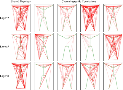
Figure 5: Visualization of the shared topologies and channel-specific correlations. The green lines show the natural connections of human skeleton. The intensity of red lines indicates the connection strength of correlations.

As shown in Figure 5, we visualize the shared topologies and channel-specific correlations of our CTR-GCN. The input sample belongs to “typing on a keyboard”. It can be seen that (1) the shared topologies in three layers tend to be coarse and dense, which captures global features for recognizing actions; (2) the channel-specific correlations varies with different channels, indicating that our CTR-GCN models individual joints relationships under different types of motion features; (3) most channel-specific correlations focus on two hands, which capture subtle interactions on hands and are helpful for recognizing “typing on a keyboard”.

Ablation Study

Number	Param.	Acc (%)
3(CTR-GCN)	1.46M	84.9
1	0.85M	84.3 ↓0.5
2	1.15M	84.7 ↓0.2
4	1.76M	85.2 ↑0.3
5	2.07M	85.4 ↑0.5
6	2.37M	85.0 ↑0.1

Table 9: Comparisons of model performances with different number of CTR-GCs.

Effect of CTR-GC’s number. In CTR-GCN, we use three CTR-GCs for fair comparison with other methods (e.g., AGCN, MSG3D), which mostly use three or more GCs to increase model capacity. To verify the effectiveness of CTR-GC’s number to our method, We test the model with 1 6 CTR-GCs. As shown in Table 9, accuracies first increase due to increased model capacity, but drops at 6 CTR-GCs, which may be caused by overfitting.

Temporal Modeling	Acc (%)
Temporal Conv(CTR-GCN)	84.9
Temporal Pooling	72.8 ↓12.1

Table 10: Comparisons of model performances with different number of CTR-GCs.

Effect of temporal convolutions. It’s a common practice to use (multi-scale) temporal convolutions for temporal modeling in skeleton-based action recognition. To validate the effect of temporal convolutions, we try to use global average pooling for temporal modeling. As shown in Table 10, the performance drops from 84.9% to 72.8%, probably because the pooling loses too much temporal information to extract joints’ trajectory features effectively.

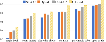
Figure 6: Comparison of classification accuracy of different graph convolutions on hard action classes.

Performance on hard classes. We further analyze the performance of different graph convolutions on hard classes on NTU-RGB+D 120, i.e., “staple book”, “count money”, “play with phone” and “cut nails”, “playing magic cube” and “open bottle”. These actions mainly involve subtle interactions between fingers, making them difficult to be recognized correctly. As shown in Figure 6, CTR-GC outperforms other graph convolutions on all classes. Especially, CTR-GC exceeds other methods at least by 7.03% and 4.36% on “cut nails” and “open bottle” respectively, showing that, compared with other GCs, our CTR-GC can effectively extract features of subtle interactions and classify them more accurately.

References

- [1] Joan Bruna, Wojciech Zaremba, Arthur Szlam, and Yann LeCun. Spectral networks and locally connected networks on graphs. arXiv preprint arXiv:1312.6203, 2013.
- [2] Yinpeng Chen, Xiyang Dai, Mengchen Liu, Dongdong Chen, Lu Yuan, and Zicheng Liu. Dynamic convolution: Attention over convolution kernels. In Proceedings of the IEEE/CVF Conference on Computer Vision and Pattern Recognition, pages 11030–11039, 2020.
- [3] Ke Cheng, Yifan Zhang, Congqi Cao, Lei Shi, Jian Cheng, and Hanqing Lu. Decoupling gcn with dropgraph module for skeleton-based action recognition. In Proceedings of the European Conference on Computer Vision (ECCV), 2020.
- [4] Ke Cheng, Yifan Zhang, Xiangyu He, Weihan Chen, Jian Cheng, and Hanqing Lu. Skeleton-based action recognition with shift graph convolutional network. In Proceedings of the IEEE/CVF Conference on Computer Vision and Pattern Recognition, pages 183–192, 2020.
- [5] Michaël Defferrard, Xavier Bresson, and Pierre Vandergheynst. Convolutional neural networks on graphs with fast localized spectral filtering. In Advances in neural information processing systems, pages 3844–3852, 2016.
- [6] Yong Du, Wei Wang, and Liang Wang. Hierarchical recurrent neural network for skeleton based action recognition. In Proceedings of the IEEE conference on computer vision and pattern recognition, pages 1110–1118, 2015.
- [7] David K Duvenaud, Dougal Maclaurin, Jorge Iparraguirre, Rafael Bombarell, Timothy Hirzel, Alán Aspuru-Guzik, and Ryan P Adams. Convolutional networks on graphs for learning molecular fingerprints. In Advances in neural information processing systems, pages 2224–2232, 2015.
- [8] Kaiming He, Xiangyu Zhang, Shaoqing Ren, and Jian Sun. Deep residual learning for image recognition. In Proceedings of the IEEE conference on computer vision and pattern recognition, pages 770–778, 2016.
- [9] Zhen Huang, Xu Shen, Xinmei Tian, Houqiang Li, Jianqiang Huang, and Xian-Sheng Hua. Spatio-temporal inception graph convolutional networks for skeleton-based action recognition. In Proceedings of the 28th ACM International Conference on Multimedia, pages 2122–2130, 2020.
- [10] Qiuhong Ke, Mohammed Bennamoun, Senjian An, Ferdous Sohel, and Farid Boussaid. Learning clip representations for skeleton-based 3d action recognition. IEEE Transactions on Image Processing, 27(6):2842–2855, 2018.
- [11] Thomas N Kipf and Max Welling. Semi-supervised classification with graph convolutional networks. arXiv preprint arXiv:1609.02907, 2016.
- [12] Matthew Korban and Xin Li. Ddgcn: A dynamic directed graph convolutional network for action recognition. In European Conference on Computer Vision, pages 761–776. Springer, 2020.
- [13] Inwoong Lee, Doyoung Kim, Seoungyoon Kang, and Sanghoon Lee. Ensemble deep learning for skeleton-based action recognition using temporal sliding lstm networks. In Proceedings of the IEEE international conference on computer vision, pages 1012–1020, 2017.
- [14] Chao Li, Qiaoyong Zhong, Di Xie, and Shiliang Pu. Co-occurrence feature learning from skeleton data for action recognition and detection with hierarchical aggregation. arXiv preprint arXiv:1804.06055, 2018.
- [15] Maosen Li, Siheng Chen, Xu Chen, Ya Zhang, Yanfeng Wang, and Qi Tian. Actional-structural graph convolutional networks for skeleton-based action recognition. In Proceedings of the IEEE/CVF Conference on Computer Vision and Pattern Recognition, pages 3595–3603, 2019.
- [16] Shuai Li, Wanqing Li, Chris Cook, Ce Zhu, and Yanbo Gao. Independently recurrent neural network (indrnn): Building a longer and deeper rnn. In Proceedings of the IEEE conference on computer vision and pattern recognition, pages 5457–5466, 2018.
- [17] Jun Liu, Amir Shahroudy, Mauricio Lisboa Perez, Gang Wang, Ling-Yu Duan, and Alex Kot Chichung. Ntu rgb+ d 120: A large-scale benchmark for 3d human activity understanding. IEEE transactions on pattern analysis and machine intelligence, 2019.
- [18] Jun Liu, Amir Shahroudy, Dong Xu, and Gang Wang. Spatio-temporal lstm with trust gates for 3d human action recognition. In European conference on computer vision, pages 816–833. Springer, 2016.
- [19] Jun Liu, Gang Wang, Ling-Yu Duan, Kamila Abdiyeva, and Alex C Kot. Skeleton-based human action recognition with global context-aware attention lstm networks. IEEE Transactions on Image Processing, 27(4):1586–1599, 2017.
- [20] Ziyu Liu, Hongwen Zhang, Zhenghao Chen, Zhiyong Wang, and Wanli Ouyang. Disentangling and unifying graph convolutions for skeleton-based action recognition. In Proceedings of the IEEE/CVF Conference on Computer Vision and Pattern Recognition, pages 143–152, 2020.
- [21] Mathias Niepert, Mohamed Ahmed, and Konstantin Kutzkov. Learning convolutional neural networks for graphs. In International conference on machine learning, pages 2014–2023, 2016.
- [22] Amir Shahroudy, Jun Liu, Tian-Tsong Ng, and Gang Wang. Ntu rgb+ d: A large scale dataset for 3d human activity analysis. In Proceedings of the IEEE conference on computer vision and pattern recognition, pages 1010–1019, 2016.
- [23] Lei Shi, Yifan Zhang, Jian Cheng, and Hanqing Lu. Skeleton-based action recognition with directed graph neural networks. In Proceedings of the IEEE Conference on Computer Vision and Pattern Recognition, pages 7912–7921, 2019.
- [24] Lei Shi, Yifan Zhang, Jian Cheng, and Hanqing Lu. Two-stream adaptive graph convolutional networks for skeleton-based action recognition. In Proceedings of the IEEE Conference on Computer Vision and Pattern Recognition, pages 12026–12035, 2019.
- [25] Chenyang Si, Wentao Chen, Wei Wang, Liang Wang, and Tieniu Tan. An attention enhanced graph convolutional lstm network for skeleton-based action recognition. In Proceedings of the IEEE conference on computer vision and pattern recognition, pages 1227–1236, 2019.
- [26] Yi-Fan Song, Zhang Zhang, Caifeng Shan, and Liang Wang. Stronger, faster and more explainable: A graph convolutional baseline for skeleton-based action recognition. In Proceedings of the 28th ACM International Conference on Multimedia, pages 1625–1633, 2020.
- [27] Yansong Tang, Yi Tian, Jiwen Lu, Peiyang Li, and Jie Zhou. Deep progressive reinforcement learning for skeleton-based action recognition. In Proceedings of the IEEE Conference on Computer Vision and Pattern Recognition, pages 5323–5332, 2018.
- [28] Vivek Veeriah, Naifan Zhuang, and Guo-Jun Qi. Differential recurrent neural networks for action recognition. In Proceedings of the IEEE international conference on computer vision, pages 4041–4049, 2015.
- [29] Petar Veličković, Guillem Cucurull, Arantxa Casanova, Adriana Romero, Pietro Lio, and Yoshua Bengio. Graph attention networks. arXiv preprint arXiv:1710.10903, 2017.
- [30] Jiang Wang, Zicheng Liu, Ying Wu, and Junsong Yuan. Learning actionlet ensemble for 3d human action recognition. IEEE transactions on pattern analysis and machine intelligence, 36(5):914–927, 2013.
- [31] Jiang Wang, Xiaohan Nie, Yin Xia, Ying Wu, and Song-Chun Zhu. Cross-view action modeling, learning and recognition. In Proceedings of the IEEE conference on computer vision and pattern recognition, pages 2649–2656, 2014.
- [32] Sijie Yan, Yuanjun Xiong, and Dahua Lin. Spatial temporal graph convolutional networks for skeleton-based action recognition. arXiv preprint arXiv:1801.07455, 2018.
- [33] Brandon Yang, Gabriel Bender, Quoc V. Le, and Jiquan Ngiam. Condconv: Conditionally parameterized convolutions for efficient inference. In Advances in Neural Information Processing Systems 32: Annual Conference on Neural Information Processing Systems 2019, NeurIPS 2019, December 8-14, 2019, Vancouver, BC, Canada, pages 1305–1316, 2019.
- [34] Fanfan Ye, Shiliang Pu, Qiaoyong Zhong, Chao Li, Di Xie, and Huiming Tang. Dynamic gcn: Context-enriched topology learning for skeleton-based action recognition. In Proceedings of the 28th ACM International Conference on Multimedia, pages 55–63, 2020.
- [35] Pengfei Zhang, Cuiling Lan, Wenjun Zeng, Junliang Xing, Jianru Xue, and Nanning Zheng. Semantics-guided neural networks for efficient skeleton-based human action recognition. In Proceedings of the IEEE/CVF Conference on Computer Vision and Pattern Recognition, pages 1112–1121, 2020.
- [36] Rui Zhao, Kang Wang, Hui Su, and Qiang Ji. Bayesian graph convolution lstm for skeleton based action recognition. In Proceedings of the IEEE/CVF International Conference on Computer Vision, pages 6882–6892, 2019.