Black-Box Diagnosis and Calibration on GAN Intra-Mode Collapse: A Pilot Study

Abstract.

Generative adversarial networks (GANs) nowadays are capable of producing images of incredible realism. One concern raised is whether the state-of-the-art GAN’s learned distribution still suffers from mode collapse, and what to do if so. Existing diversity tests of samples from GANs are usually conducted qualitatively on a small scale, and/or depends on the access to original training data as well as the trained model parameters. This paper explores to diagnose GAN intra-mode collapse and calibrate that, in a novel black-box setting: no access to training data, nor the trained model parameters, is assumed. The new setting is practically demanded, yet rarely explored and significantly more challenging. As a first stab, we devise a set of statistical tools based on sampling, that can visualize, quantify, and rectify intra-mode collapse. We demonstrate the effectiveness of our proposed diagnosis and calibration techniques, via extensive simulations and experiments, on unconditional GAN image generation (e.g., face and vehicle). Our study reveals that the intra-mode collapse is still a prevailing problem in state-of-the-art GANs and the mode collapse is diagnosable and calibratable in black-box settings. Our codes are available at: https://github.com/VITA-Group/BlackBoxGANCollapse.

1. Introduction

Generative adversarial networks (GANs) (Goodfellow et al., 2014; Karras et al., 2017, 2018; Karras et al., 2019; Arjovsky et al., 2017; Mao et al., 2017; Wu et al., 2020a; Gong et al., 2019; Jiang et al., 2021b; Kupyn et al., 2019; Jiang et al., 2021a; Wang et al., 2020a; Yang et al., 2021, 2019, 2020) have demonstrated unprecedented power for image generation. However, GANs suffer from generation bias and/or loss of diversity. The underlying reasons could be compound, ranging from the data imbalance to the training difficulty, and more:

• First, the training data for GANs, e.g., for the most-studied unconditional/unsupervised generation tasks (Karras et al., 2017, 2018), could possess various subject or attribute imbalances (Wang et al., 2020b). Consequently, GANs trained with them might be further biased towards the denser areas, similarly to the classifier bias towards the majority class in imbalanced classification.

• More intrinsically, even when the training data “looks” balanced, training GANs is much more unstable and uncontrollable than training classifiers. One common hurdle of GANs is the loss of diversity due to mode collapse (Goodfellow, 2016), wherein the generator concentrates a probability mass on only a few modes of the true distribution. It is often considered as a training artifact. Another widely reported issue, covariate shift (Santurkar et al., 2017), could be viewed as a nuanced version of mode collapse.

1.1. Diversity Evaluation of GANs

There are several popular metrics for evaluation, e.g., Inception Score (IS) (Salimans et al., 2016), Fréchet Inception Distance (FID) (Heusel et al., 2017), MODE (Che et al., 2016) and birthday paradox test (Arora and Zhang, 2017). However, they are not always sensitive to mode collapses; see Section 2.1 for more discussions.

Recently, two classification-based metrics (Santurkar et al., 2017; Bau et al., 2019) have been proposed for quantitatively assessing the mode distribution learned by GANs by comparing the learned distribution of attributes or objects in the generated images with the target distribution in the training set. However, Santurkar et al. (Santurkar et al., 2017) hinges on a classifier trained on the original (and manually balanced) GAN training set, with class labels known, available, and well-defined (e.g., object classes in CIFAR-10, or facial attributes in CelebA); Bau et al. (Bau et al., 2019) relies on an instance segmentation model trained on images with $336$ object classes. They mainly focus on detecting the mode collapse measured at class level but do not directly address the mode collapse within a class.

Mode collapse refers to the limited sample variety in the generator’s learned distribution. As discussed by Huang et al. (Huang et al., 2018), inter-mode collapse occurs when some modes (e.g., digit classes in MNIST) are never produced from the generated samples; while intra-mode collapse occurs when all modes (e.g., classes) can be found in the generated samples but with limited variations (e.g., a digit with few writing styles). Both types of mode collapses are commonly observed in GANs, and the above classification-based metrics, by definition, can only detect the inter-mode collapse. Also, they cannot be easily extended to images subjects where classes are not well defined and/or not enumerable (e.g., the identity of generated faces/vehicles, or in other open set problems).

Beyond the above progress, many open questions persist, including but not limited to: do state-of-the-art GANs still suffer from intra-mode collapse? Can we detect it with minimal assumptions or efforts? Moreover, whether there is an “easy and quick” remedy to alleviate it? – Addressing them motivates our work.

1.2. Black-Box Diagnosis & Calibration

Many approaches have been proposed to alleviate mode collapse, ranging from better optimization objectives (Arjovsky et al., 2017; Mao et al., 2017) to customized building blocks (Durugkar et al., 2016; Ghosh et al., 2018; Liu and Tuzel, 2016; Lin et al., 2018). However, they require either specialized GAN architectures and/or tedious (re-)training, or at least access to training data and/or model parameters. Whether it is for diagnosing (detecting or evaluating) mode collapse, or calibrating (alleviating or fixing) it, all the above methods require the original training data and/or the trained model parameters. We refer to those methods as white-box approaches.

In contrast, the main goal of this work is to significantly extend the applicability of such diagnosis and calibration to an almost unexplored black-box setting: we assume neither access to the original training data, nor the model parameters, nor the class labels of the original data (which might be inaccessible or even not well defined, as above explained). To our best knowledge, no existing approach is immediately available to address this new challenge. Instead, we find such black-box setting desired by practitioners due to the following reasons: (i) the training data might be protected or no longer available since it contains sensitive information (e.g., human faces or person images); (ii) the GAN model might be provided as a black box and cannot be modified (e.g., as commercial IPs, executables, or APIs); (iii) the practitioners want to adjust the generated distribution of any GAN without expensive re-training, to enable fast turn-around and also save training resources.

Assume, for just one example, a GAN model is protected by IP and provided to users as an executable (or cloud API) only. The black-box diagnosis and calibration are helpful for both the users and the provider. For the users, they could effectively discover whether the provided API displays any unexpected generation deficiency or bias, despite having no access to the weights nor data. For the provider, they could identify a collapse and quickly fix it, by adding merely light-weight “wrapping” (e.g., output post-processing) to the model, instead of costly (even infeasible) re-training.

1.3. Our Contributions

As a first stab at this new challenge, we propose hypothesis testing methods to analyze the clustering density pattern of generated samples. To characterize point patterns over a given area of interest, we incorporate statistical tools in spatial analysis and the Monte Carlo method to provide both qualitative and quantitative measures of mode collapse. Then, for the first time, we explore two black-box approaches to calibrate the GAN’s learned distribution and to rectify the detected mode collapse, via Gaussian mixture models and importance sampling, respectively. It is crucial to notice that neither the proposed diagnosis nor the calibrations touch the original training data, access the model parameters, or re-train the model in any way: they are all based on sampling from the “black box”.

We demonstrate the application of our new toolkit in analyzing the intra-mode collapse in unconditional image generation tasks, such as face and vehicle images. Instead of measuring a “global” class distribution, our method focuses on addressing “local” high-density regions. Therefore, it is specialized at detecting the intra-mode collapse, and is complementary to (Santurkar et al., 2017) and (Bau et al., 2019). We find the intra-mode collapse remains a prevailing problem in state-of-the-art GANs (Karras et al., 2018, 2017; Brock et al., 2018; Karras et al., 2019). We analyze several possible causes and demonstrate our calibration approaches can notably alleviate the issue.

Although beyond our discussion scope, we point out that our proposed diagnosis and calibration on intra-mode collapse can contribute to understanding the privacy (Filipovych et al., 2011; Zheng et al., 2020; Wu et al., 2018, 2020b) and fairness (Holstein et al., 2018; Wu et al., 2019; Uplavikar et al., 2019) issues in generative models. First, the collapsed mode in GAN’s learned distribution, i.e., images of repeated identity, could focus on some training data, especially when the data is highly imbalanced, thus causing privacy breach if the training data is protected. Second, the collapsed mode shows the generative model’s bias towards some specific identities. Many existing works using generated synthetic images together with or instead of real images for training, with their purposes ranging from semi-supervised learning (Salimans et al., 2016) to small data augmentation (Bowles et al., 2018; Liu et al., 2019; Zhang et al., 2019). As a potential consequence, training with the generated data might incur biased classifier predictions.

2. Related Works

2.1. Privacy and Fairness Concerns in GANs

2.1.1. Privacy

The privacy breach risk of GANs lies in generating data that are more likely to be substantially similar to existing training samples, as a consequence of potential overfitting. Xie et al. (Xie et al., 2018) argues that the density of the learned distribution could overly concentrate on the training data points, which is alarming when the training data is private or sensitive. The authors proposed to train a differential private GAN (DPGAN) by gradient noise injection and then to clip. Webster et al. (Webster et al., 2019) studies GAN’s overfitting issue by analyzing the statistics of reconstruction errors on both training and validation images, by optimizing the latent code to find the nearest neighbor in the generation manifold. Their empirical study finds out that standard GAN evaluation metrics often fail to capture memorization for deep generators, making overfitting undetectable for pure GANs and causing privacy leak risks.

2.1.2. Fairness

Amini et al. (Amini et al., 2019) propose an debiasing VAE (DB-VAE) algorithm, on mitigating generation bias, but it needs a large dataset to learn its latent structure. Xu et al. (Xu et al., 2018) develops FairGAN for fair data generation, which achieves statistical parity with regard to a protected attribute, using an auxiliary discriminator to ensure no correlation between protected/unprotected attributes, as well as between the utility task and the protected attribute. Sattigeri et al. (Sattigeri et al., 2018) also aimed to generate debiased, fair data to protected attributes in allocative decision making, with a pair of auxiliary losses introduced to encourage demographic parity. Unlike those existing works, we seek to analyze and gain insights into the fairness issue in current state-of-the-art GANs (rather than specifically crafted ones), where currently no fairness constraint has not been, or is non-trivial to be enforced.

2.2. Evaluation of Mode Collapse in GANs

GANs are often observed to suffer from the mode collapse problem (Salimans et al., 2016; Sutskever et al., 2015), where only a small subset of distribution modes are characterized by the generator. The problem is especially prevalent for high-resolution image generation, where the training samples are low-density w.r.t. the high-dimensional feature space. Salimans et al. (Salimans et al., 2016) presented the popular metric of Inception Score (IS) to measure the individual sample quality. IS does not directly reflect the population-level generation quality, e.g., the overfitting, and loss of diversity. It also requires pre-trained perceptual models on ImageNet or other specific datasets (Barratt and Sharma, 2018). Heusel et al. (Heusel et al., 2017) proposed the Fréchet Inception Distance (FID), which models the distribution of image features as multivariate Gaussian distribution and computes the distance between the distribution of real and fakes images. Unlike IS, FID can detect intra-class mode dropping. However, as pointed out by Borji et al. (Borji, 2019), the multivariate Gaussian distribution assumption does not hold well on real images, limiting FID’s trustworthiness. Besides IS and FID, Che et al. (Che et al., 2016) developed an assessment for both visual quality and variety of samples, known as MODE score, and later shown to be similar to IS (Zhou et al., 2017). Arora et al. (Arora et al., 2018; Arora and Zhang, 2017) proposed a test based upon the birthday paradox for estimating the support size of the generated distribution. Although the test can detect severe cases of mode collapse, it falls short in measuring how well a generator captures the true data distribution. It also heavily relies on human annotation, thus hard to scale up to larger-scale evaluation. Santurkar et al. (Santurkar et al., 2017) and Bau et al. (Bau et al., 2019) are the closet existing works to to our proposed diagnosis. Both approaches took a classification-based perspective and regarded the loss of diversity as a form of covariate shift. Unfortunately, as discussed above, their approaches are “white box” and depend on the exposure of original training data. Also, their approaches cannot be extended to subjects without well-defined class labels.

2.3. Model Calibration for GANs

There are many efforts addressing the mode collapse problem in GANs. Some focus on discriminators by introducing different divergence metrics (Metz et al., 2016) and optimization losses (Arjovsky et al., 2017; Mao et al., 2017). The minibatch discrimination scheme proposed by Salimans et al. (Salimans et al., 2016) allows discrimination between whole mini-batches of samples instead of between individual samples. Durugkar et al. (Durugkar et al., 2016) adopted multiple discriminators to alleviate mode collapse. Lin et al. (Lin et al., 2018) proposed PacGAN to mitigate mode collapse by passing $m$ “packed” or concatenated samples to the discriminator for joint classification.

ModeGAN (Che et al., 2016) and VEEGAN (Srivastava et al., 2017) enforce the bijection mapping between the input noise vectors and generated images with additional encoder networks. Multiple generators (Ghosh et al., 2018) and weight-sharing generators (Liu and Tuzel, 2016) are developed to capture more modes of the distribution. However, all of the above assumes (re-)training, and hence are on a different track from our work that focuses on calibrating trained GANs as “black boxes”.

A handful of works attempted to apply sampling methods to improve GAN generation quality. Turner et al. (Turner et al., 2018) introduced the Metropolis-Hastings generative adversarial network (MH-GAN). MH-GAN uses the learned discriminator from GAN training to build a wrapper for the generator for improved sampling at the generation inference stage. With a perfect discriminator, the wrapped generator can sample from the true distribution exactly even with a deficient generator. Azadi et al. (Azadi et al., 2018) proposed discriminator rejection sampling (DRS) for GANs, which rejects the generator samples by using the probabilities given by the discriminator to approximately correct errors in the generator’s distribution. Nevertheless, these approaches are white-box calibration and require access to trained discriminators, which are hardly accessible or even discarded after a GAN is trained.

3. Method

Inter-Mode Collapse vs. Intra-Mode Collapse. Mode collapse happens when there are at least two distant points in the code vector $\mathcal{Z}$ mapped to the same or similar points in the sample space $\mathcal{X}$, whose consequence is limited sample variety in $\mathcal{X}$. There are two distinct concepts here: intra-mode collapse and inter-mode collapse. Inter-mode collapse occurs when some modes (e.g., digit classes in MNIST) are never produced from the generated samples; while intra-mode collapse occurs when all modes (e.g., classes) can be found in the generated samples but with limited variations (e.g., a digit with few writing styles). In this paper, we investigate the intra-mode collapse on the task of unconditional GAN image generation, due to its popularity as well as the constraint of missing object labels during generation. Note that all our techniques can be straightforwardly applied to a conditional generation too.

Given an unconditional generator $G$, we can sample an image $\mathcal{I}=G(z)$ by drawing $z$ from a standard Gaussian distribution $\mathbb{N}(z)$. We define that mode collapse happens when the probability of generating samples with a certain condition $f(\mathcal{I}){=}0$ deviates from the expected value of a target distribution.

For inter-mode collapse, the conditional function $f$ usually specifies the probability of $\mathcal{I}$ belonging to a certain class (Santurkar et al., 2017; Bau et al., 2019). For intra-mode collapse, we favor a conditional function $f$ that can characterize the diversity of samples in a local region. The definition of diversity (loss), especially when it comes to the semantic level, can be elusive and vague. To concretize our study subject, we focus on the collapse of the most significant property that makes a generated image “unique”, i.e., the identity (for generated faces, vehicle, etc.). Note that the definition of identity generalizes more broadly than class, and can apply to open-set scenarios when the class is not well-defined, such as generating new faces. Conceptually, we can measure intra-mode collapse w.r.t. an anchor image $\mathcal{I}^{\prime}$ by the probability of generating a sample $\mathcal{I}$ with the same identity as $\mathcal{I}^{\prime}$, i.e., $f(\mathcal{I})=ID(\mathcal{I}^{\prime})-ID(\mathcal{I})$.

Black-Box Setting. We assume neither access to the original training data, nor the model parameters, nor the class labels of the original data (which might be inaccessible or even not well defined, as above explained).

Diagnosis & Calibration. Importantly, we never use the identity labels in any form to evaluate sample diversity. Instead, we leverage the embedded features obtained from the deep networks pre-trained for the recognition or re-identification task for subjects such as faces and vehicles. That is based on the known observation that those “identity” features can often directly characterize or show strong transferability to depict other essential attributes: e.g., age/gender/race of faces (Savchenko, 2019) and color/type/brand of vehicles (Zheng et al., 2019).

Assume we have an identity descriptor $F_{id}(\cdot)$ that produces a unit vector for image $\mathcal{I}$ in the identity embedding space. We can use the identity feature similarity $s(\mathcal{I}^{\prime},\mathcal{I})$ between the anchor and sampled images as a probabilistic surrogate to identity matching in our conditional function:

(1) $$f(\mathcal{I})\sim\mathbb{B}(s(\mathcal{I}^{\prime},\mathcal{I})),$$

where $\mathbb{B}(p)$ denotes Bernoulli distribution with zero-probability $p$. Thus, the detection metric for our intra-mode collapse becomes the expected similarity with the anchor image $\mathcal{I}^{\prime}$:

(2) $$p(f(\mathcal{I})=0)=\mathbf{E}_{\mathcal{I}}[s(\mathcal{I}^{\prime},\mathcal{I})].$$

Since only high similarity indicates possible identity matching, we design $s(\cdot,\cdot)$ as a truncated exponential function of inverse feature distance:

(3) $$s(\mathcal{I}_{1},\mathcal{I}_{2})=\frac{1}{e^{\theta}-1}(e^{max(0,\theta-d(\mathcal{I}_{1},\mathcal{I}_{2}))}-1),$$

where $d(\cdot,\cdot)$ is the normalized cosine distance between identity features:

(4) $$d(\mathcal{I}_{1},\mathcal{I}_{2})=\frac{1}{\pi}cos^{-1}(<F_{id}(\mathcal{I}_{1}),F_{id}(\mathcal{I}_{2})>),$$

and $\theta$ is a hyper-parameter specifying the maximum feature distance between two images of the same identity in the embedding space $F_{id}$. Note that $\theta$ only depends on $F_{id}$. We use Monte Carlo sampling to approximate the expected similarity between an anchor image $\mathcal{I}^{\prime}$ and a randomly sampled image in the generator’s learned distribution. We further propose two calibration approaches to alleviate the collapse by “reshaping the latent space”.

3.1. Black-box Intra-Mode Collapse Diagnosis via Monte Carlo Sampling

Now we introduce a practical way to evaluate the expected similarity between an anchor image $\mathcal{I}^{\prime}$ and a randomly sampled image $\mathcal{I}{=}G(z)$:

(5) $$\begin{array}[]{l}\mathbf{E}_{z}[s(\mathcal{I}^{\prime},G(z))]=\bigintssss_{z}s(\mathcal{I}^{\prime},G(z))p(z)dz.\end{array}$$

Eq.(5) can be used to quantitatively measure the mode collapse in the neighborhood of the anchor $\mathcal{I}^{\prime}$ in $G$’s learned distribution. We hereby show two extreme cases: Eq.(5) yields $0$ when $G$ produces no images similar to $\mathcal{I}^{\prime}$ (i.e., $\forall z,d(G(z),\mathcal{I}^{\prime})>\theta$); in contrast, Eq.(5) yields $1$ when $G$ produces identical images to $\mathcal{I}^{\prime}$ (i.e., $\forall z,d(G(z),\mathcal{I}^{\prime})=0$).

As the integral in Eq.(5) is generally intractable, we further incorporate Monte Carlo sampling to approximate the expectation with the average of $n$ samples from a Gaussian distribution $\{z_{i}\}\sim\mathbb{N}(z)$:

(6) $$\mathbf{E}_{z}[s(\mathcal{I}^{\prime},G(z))]\approx\frac{1}{n}\displaystyle\sum_{i=1}^{n}s(\mathcal{I}^{\prime},G(z_{i})).$$

Considering both scale and normalization in Eq.(6), we further define a metric named “Monte Carlo-based Collapse Score” (MCCS):

(7) $$\textit{MCCS}(\mathcal{I}^{\prime})=1/(1-\log(\frac{1}{n}\displaystyle\sum_{i=1}^{n}s(\mathcal{I}^{\prime},G(z_{i})))),$$

where $n$ is the size of $\mathcal{C}$, a collection of sampled images. MCCS ranges between $0$ and $1$: the larger it is, the more $G$ suffers in mode collapse on $\mathcal{I}^{\prime}$. In Section 4.2, we empirically validate the sampling-efficiency and effectiveness of the proposed MCCS.

Finally, the population statistics of MCCS can indicate the occurrence of local dense modes in the entire sample space. We use the mean $\mu_{\text{mccs}}$ and the standard deviation $\sigma_{\text{mccs}}$ of MCCS to quantitatively measure GANs’ intra-mode collapse:

(8) $$\begin{split}\mu_{\text{mccs}}=\frac{1}{m}\displaystyle\sum_{i=1}^{m}\textit{MCCS}(G(z_{i})),\sigma_{\text{mccs}}=(\displaystyle\sum_{i=1}^{m}\frac{(\textit{MCCS}(G(z_{i}))-\mu_{\text{mccs}})^{2}}{m-1})^{1/2}.\end{split}$$

Note that, to get the population statistics, we need to obtain a collection of sampled anchor images $\mathcal{A}$, whose size is $m$. We have $\mathcal{A}\cap\mathcal{C}=\varnothing$. Details are shown in Section 4.2.1.

(a) $|\mathcal{A}|=1k$

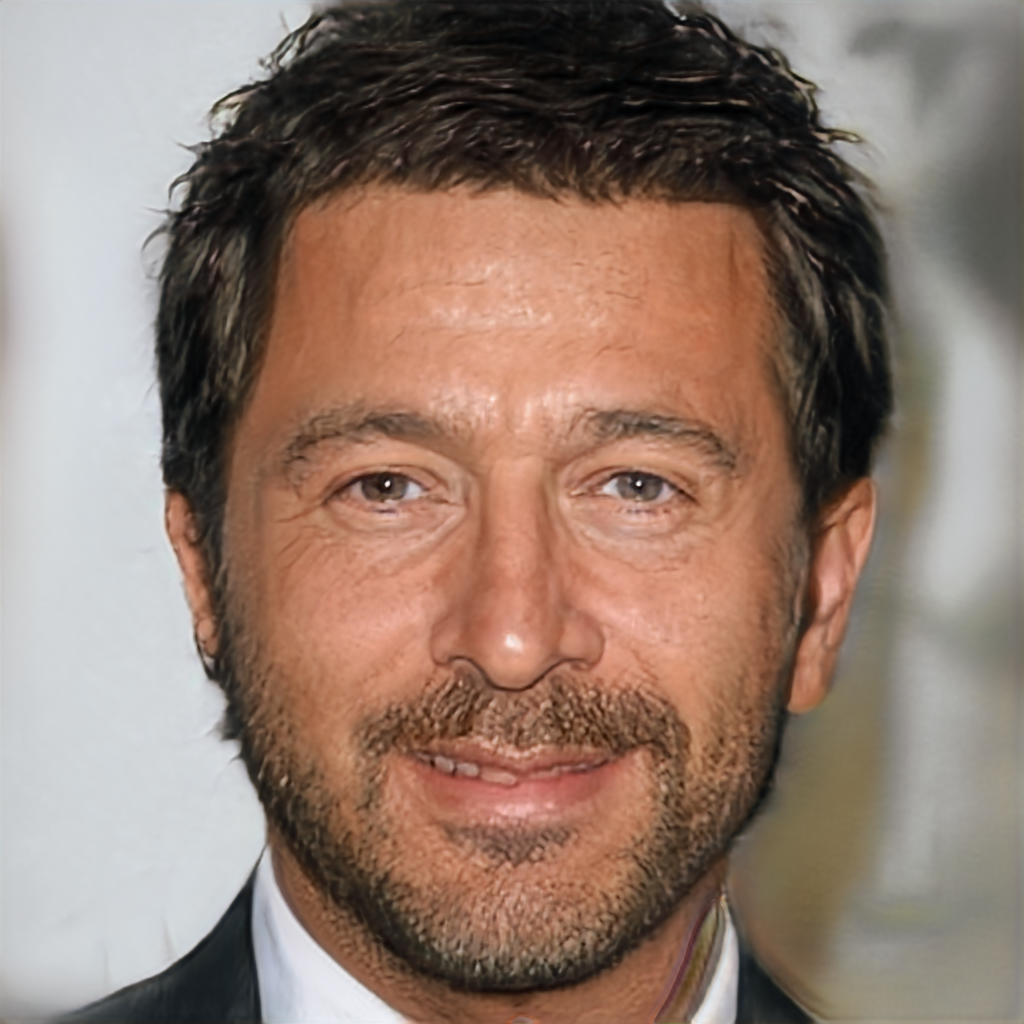
(b) $|\mathcal{A}|=10k$

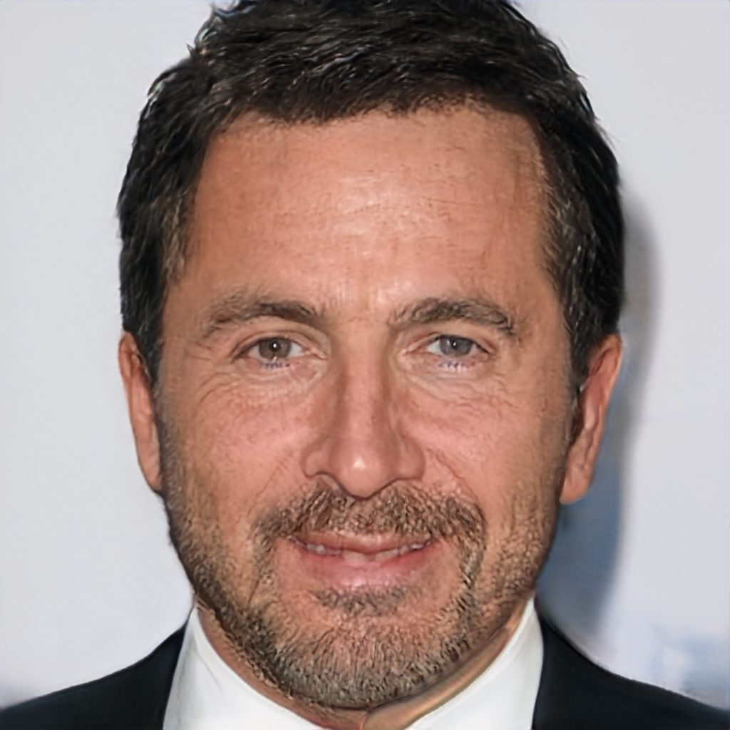
(c) $|\mathcal{A}|=100k$

(d) $|\mathcal{A}|=1m$

(e) $|\mathcal{A}|=10m$

Figure 1. Visualization of the worst-case dense mode $\mathcal{I}_{w}$ w.r.t. different size of the $\mathcal{A}$. $\mathcal{A}$ is a collection of randomly sampled anchor images. The $\mathcal{I}_{w}$ could be reliable obtained when $|\mathcal{A}|=10k$.

3.2. Black-box Intra-Mode Collapse Calibration via Latent Space Reshaping

3.2.1. Calibration w.r.t. the “Worst-Case" Collapse

In calibration, we first define the worst-case collapsed (dense) mode $\mathcal{I}_{w}$, i.e., the identity with the largest number of neighbors within a specified distance threshold. Given the radius $r$ of the points neighborhood centered at $\mathcal{I}^{\prime}$ in the embedding space, a collection of randomly sampled anchor images $\mathcal{A}$, a collection of randomly sampled images $\mathcal{C}$, a worst-case collapsed mode $\mathcal{I}_{w}$ can be expressed as:

(9) $$\mathcal{I}_{w}=\operatorname*{arg\,max}_{\mathcal{I}^{\prime}\in\mathcal{A}}\displaystyle\sum_{\mathcal{I}\in\mathcal{C}}\mathbf{1}_{r}(d(\mathcal{I}^{\prime},\mathcal{I})),$$

where $\sum_{\mathcal{I}\in\mathcal{C}}\mathbf{1}_{r}(d(\mathcal{I}^{\prime},\mathcal{I}))$ computes the number of neighbors within $r$ distance of $\mathcal{I}^{\prime}$ in the embedding space, among all images in $\mathcal{C}$, and $\mathbf{1}_{r}(\cdot)$ is an indicator function that gives $1$ if $d(\mathcal{I}^{\prime},\mathcal{I})\leq r$.

Algorithm 1 Reshaping Latent Space via Gaussian Mixture Models

$\triangleright$ Given a generator $G$, a neighbor distance threshold $r_{0}$, and a collection of dense modes $\mathcal{D}$

$\triangleright$ $\mathcal{Z}$ $\leftarrow$ $\{z_{1},\cdots,z_{n}\}$ // $n$ sampled latent codes

$\triangleright$ $\{\mu_{k}\}_{K},\mathbf{A}_{c}(\cdot)\leftarrow\text{K-Means}(\mathcal{Z},K)$ // Cluster assignment $\mathbf{A}_{c}:\mathcal{Z}\mapsto\{1,\cdots,K\}$

$\triangleright$ $w_{sum}\leftarrow 0$ // The normalization factor

for each $k\in\text{range}(1,K)$ do

     $\triangleright$ $\mathcal{C}_{k}\leftarrow\{G(z)|\mathbf{A}_{c}(z)=k,z\in\mathcal{Z}\}$

     $\triangleright$ $w_{k}\leftarrow 1/(\sum_{\mathcal{I}_{m}\in\mathcal{D}}\sum_{\mathcal{I}\in\mathcal{C}_{k}}\mathbf{1}_{r_{0}}(d(\mathcal{I}_{m},\mathcal{I})))$

     $\triangleright$ $w_{sum}\leftarrow w_{sum}+w_{k}$

return $\displaystyle\sum_{k=1}^{K}\frac{w_{k}}{w_{sum}}\phi(\cdot|\mu_{k},\Sigma)$

We next present two black-box approaches, both focusing on calibrating a detected worst-case “collapsed” mode $\mathcal{I}_{w}$. The calibration aims to maximally alleviate the density of the mode $\mathcal{I}_{w}$ while preserving the overall diversity and quality of all generated images.

Biased Anchor Images. The sampled anchor images could indeed be biased due to limited sampling size. But we have empirically verified that the worst-case dense mode $\mathcal{I}_{w}$ is consistent against sampling. In order to verify the consistency of the worst-case dense mode $\mathcal{I}_{w}$ against sampling, we fix the size of $\mathcal{C}$ to be $1m$ and visualize the $\mathcal{I}_{w}$ w.r.t. different size of $\mathcal{A}$ in Figure 1. We consistently observe roughly the same identity as the sampling size increases. Therefore, despite sampling bias in anchor images, $\mathcal{I}_{w}$ can be reliably obtained even when $|\mathcal{A}|=10k$. The consistency of $\mathcal{I}_{w}$ demonstrates that the support size of $\mathcal{I}_{w}$ is nonnegligible. The experiments are conducted on StyleGAN2 trained on CelebAHQ-1024.

Why Calibrating the Worst-Case Mode Only? We emphasize that our proposed methods can be readily applied to any amounts of collapse modes; however, we have two-fold rationales: (1) focusing on and calibrating the worst-case mode provides good proofs-of-concept and are usually the easiest to demonstrate quantitative and visual gains; (2) we empirically observe that calibrating only the worst-case mode could simultaneously alleviate other collapsed modes, without incurring multiple rounds of sampling overheads.

3.2.2. Two Approaches

Given the worst-case dense mode $\mathcal{I}_{w}$, our proposed calibration approaches alleviate the collapse by “reshaping the latent space”: they operate on the latent codes as post-processing and require no modification of the trained model nor access to the model parameters or training data, making them completely “black-box”.

A prerequisite for the proposed calibrations is a smooth manifold assumption that comes from empirical observation: as we consistently obtain neighbors that are visually close to $\mathcal{I}_{w}$, when interpolating near $\mathcal{I}_{w}$, the latent codes of $\mathcal{I}_{w}$ are assumed to lay on some smooth manifold. This assumption is mild and well observed in practice.

Approach #1: Reshaping Latent Space via Gaussian Mixture Models. Based on the smooth manifold assumption, the latent space distribution $\phi(z;\xi_{0})$ can be approximated with a mixture of Gaussians $\displaystyle\sum_{i=1}^{K}w_{i}\phi(z;\xi_{i})$. We randomly sample $N$ latent codes and use $K$-means to explore $\xi_{k}=(\mu_{k},\sigma_{k})$. We denote $p(\mathcal{I}_{w})$ as the probability of sampling the target worst-case dense mode $\mathcal{I}_{w}$:

(10) $$\begin{split}p(\mathcal{I}_{w})&=\bigintssss p(\mathcal{I}_{w}|z)\phi(z;\xi_{0})dz\approx\displaystyle\sum_{k=1}^{K}w_{k}\bigintssss p(\mathcal{I}_{w}|z)\phi_{k}(z;\xi_{k})dz.\end{split}$$

If $p(\mathcal{I}_{w}|\xi_{k})$ is large, we reduce $w_{k}$ to make the overall $p(\mathcal{I}_{w})$ small. $p(\mathcal{I}_{w}|\xi_{k})$ is estimated by the number of neighbors within $r$ distance to $\mathcal{I}_{w}$ in the $k_{th}$ cluster $\mathcal{C}_{k}$, i.e., $\sum_{\mathcal{I}\in\mathcal{C}_{k}}\mathbf{1}_{r}(d(\mathcal{I}_{w},\mathcal{I}))$. The detailed algorithm is outlined in Algorithm 1.

Algorithm 2 Reshaping Latent Space via Importance Sampling

$\triangleright$ Given a generator $G$, a neighbor distance threshold $r_{0}$, and a collection of dense modes $\mathcal{D}$

$\triangleright$ $\mathcal{Z}$ $\leftarrow$ $\{z_{1},\cdots,z_{n}\}$ // $n$ sampled latent codes

$\triangleright$ $\mathcal{X}\leftarrow\{G(z_{1}),\cdots,G(z_{n})\}$

$\triangleright$ $\mathcal{I}_{r}\leftarrow G(z)$ // Random image for reference

$\triangleright$ $\text{IS}\leftarrow\varnothing$ // A collection of important sampling parameters

for each $\mathcal{I}_{m}\in\mathcal{D}$ do

     $\triangleright$ $p\leftarrow\sum_{\mathcal{I}\in\mathcal{X}}\mathbf{1}_{r_{0}}(d(\mathcal{I}_{r},\mathcal{I}))/\sum_{\mathcal{I}\in\mathcal{X}}\mathbf{1}_{r_{0}}(d(\mathcal{I}_{m},\mathcal{I}))$

     $\triangleright$ $\mathcal{H}\leftarrow\{z|d(G(z),\mathcal{I}_{m})\leq r_{0},z\in\mathcal{Z}\}$

     $\triangleright$ $\mathcal{Z}^{\prime}\leftarrow\{\displaystyle\sum_{i}\alpha_{i}z_{i}:z\in\mathcal{H},\ \forall i,\alpha_{i}\geq 0,\ \displaystyle\sum_{i}\alpha_{i}=1\}$

     $\triangleright$ $\text{IS}\leftarrow\text{IS}\cup(p,\mathcal{Z}^{\prime})$

return IS

Approach #2: Reshaping Latent Space via Importance Sampling. Under the same smooth manifold hypothesis, the high-density region corresponding to the target dense mode $\mathcal{I}_{w}$ can be approximated with a convex hull.

Let the estimated neighboring function densities for the dense and sparse regions be $p_{1}$ and $p_{2}$ respectively. We accept the samples from $G$ falling in the high-density region with a probability of $p_{2}/p_{1}$ so that the calibrated densities can match. We approximate the high-density region with a convex hull formed by the collection of latent codes corresponding to the identities close to the target dense mode $\mathcal{I}_{w}$. The details are outlined in Algorithm 2.

Compared to Approach #1 that relies on Gaussian mixture models, Approach #2 that relies on importance sampling is often found to be better in preserving the image generation quality. In importance sampling, the high-density region corresponding to the target dense mode $\mathcal{I}_{w}$ is approximated with a convex hull formed by the collection of the latent codes, whose identity is very close to $\mathcal{I}_{w}$ in the embedding space. Then, a rejection step is introduced to match the calibrated dense mode with a regular mode. In comparison, in the Gaussian mixture model, there is no explicit formulation of the dense region corresponding to the dense mode $\mathcal{I}_{w}$. However, the rejection step based on the explicit formulation of the dense mode via convex hull in the importance sampling approach brings additional computation cost, thus more time-consuming than the mixture model-based approach. We present both options for practitioners to choose from as per their needs.

4. Experiments

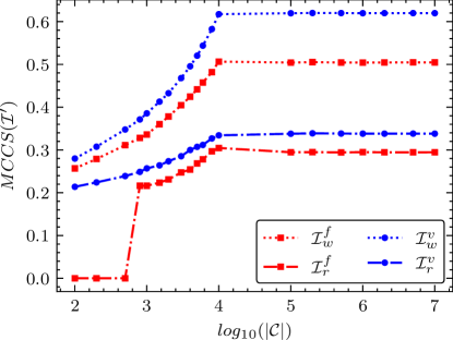
Figure 2. Justifying the sampling-efficiency of $\textit{MCCS}(\mathcal{I}^{\prime})$ w.r.t. $\log_{10}(|\mathcal{C}|)$. $|\mathcal{C}|$ is the number of sampled images. For simplicity, $\mathcal{I}_{w}$ is the worst-case dense mode. $\mathcal{I}_{r}$ is a randomly sampled image. MCCS can be reliably obtained at around $|\mathcal{C}|=10^{4}$. On the face generation task, we have $\textit{MCCS}(\mathcal{I}_{w}^{f})=0.62$ and $\textit{MCCS}(\mathcal{I}_{r}^{f})=0.34$. On the vehicle generation task, we have $\textit{MCCS}(\mathcal{I}_{w}^{v})=0.50$ and $\textit{MCCS}(\mathcal{I}_{r}^{v})=0.30$.

4.1. Experiment Settings

4.1.1. Datasets and Models

We choose four state-of-the-art GANs: PGGAN (Karras et al., 2017), StyleGAN (Karras et al., 2018) StyleGAN2 (Karras et al., 2019) and BigGAN (Brock et al., 2018), as our model subjects of study . All are known to be able to produce high-resolution, realistic, and diverse images. The observations below drawn from the four models also generalize to a few other GAN models. We choose high-resolution human face benchmarks of CelebAHQ (Karras et al., 2017) and FFHQ (Karras et al., 2018), and high-resolution vehicle benchmark of LSUN-Car (Yu et al., 2015) as our data subject of study. All benchmarks consist of diverse and realistic images. Lower resolutions are used for fast convergence in training. E.g., CelebAHQ-128 stands for CelebAHQ downsampled to $128\times 128$ resolution.

4.1.2. Choice of $F_{id}$ and Hyperparameters

We use InsightFace (Deng et al., 2019b; Guo et al., 2018; Deng et al., 2018; Deng et al., 2019a) and RAM (Liu et al., 2018) as $F_{id}$ to serve as the face identity descriptor and vehicle identity descriptor, respectively. We emphasize that the due diligence of “sanity check” has been performed on those classifiers.

4.2. Justifying MCCS’s Sampling-efficiency and Correctness

We justify the sampling-efficiency and correctness of MCCS in Eq.(7) on StyleGAN trained on CelebAHQ-$1024$ and BigGAN trained on LSUN-Car-$1024$.

4.2.1. Sampling-efficiency

We empirically justify the efficiency of sampling at both sample and population levels.

Sample-level. We first obtain two pairs of worst-case dense mode defined in Eq.(9) and a randomly sampled image on the face generation task and vehicle generation task respectively, i.e., $(\mathcal{I}_{w}^{f},\mathcal{I}_{r}^{f})$ on face and $(\mathcal{I}_{w}^{v},\mathcal{I}_{r}^{v})$ on vehicle. Then, we compute MCCS using a collection of sampled images $\mathcal{C}$ at different sizes. As is shown in Figure 2, MCCS can be reliably obtained at around $|\mathcal{C}|=10^{4}$ for $(\mathcal{I}_{w},\mathcal{I}_{r})$ on both face and vehicle generation.

Population-level. We first obtain a collection of sampled anchor images $\mathcal{A}$. Then, we draw another collection of sampled images $\mathcal{C}$. Note that $\mathcal{A}\cap\mathcal{C}=\varnothing$. Next, for each anchor image $\mathcal{I}^{\prime}\in\mathcal{A}$, we compute its value of MCCS in $\mathcal{C}$. Finally, we compute $(\mu_{\text{mccs}},\sigma_{\text{mccs}})$ using $\mathcal{A}$ and $\mathcal{C}$ at different sizes. As is shown in Figure 3, $(\mu_{\text{mccs}},\sigma_{\text{mccs}})$ can be reliably obtained at $|\mathcal{C}|=10^{4}$ and $|\mathcal{A}|=10^{4}$.

4.2.2. Correctness

We empirically justify the correctness of the proposed metric in three experiments: StyleGAN trained on a simulated image set, StyleGAN trained on CelebAHQ, and PacGAN trained on CelebA.

StyleGAN Trained on a Simulated Image Set. The first experiment is designed to prove that our proposed black-box diagnosis can uniquely detect intra-mode collapse cases, when existing evaluation metrics fail to do so. To this end, we curate a new dataset of images, whose “ground-truth collapses” are manipulated by us in a fully controlled way. No GAN-generated image is used.

CelebAHQ is a highly imbalanced dataset: among it, $30k$ high-resolution face images of $6,217$ different celebrities, the largest identity class has $28$ images, and the smallest one has only 1. Among the $30k$ faces in CelebAHQ, $20,472$ are White, $4,364$ are Black and $3,154$ are Asian. Flickr-Faces-HQ Dataset (FFHQ) is another high-quality human face dataset, consisting of $70k$ high-resolution face images, without repeated identities (we manually examined the dataset to ensure so. It is thus “balanced” in terms of identity, in the sense that each identity class has one sample. Among the $70k$ faces in FFHQ, $53,481$ are White, $9,381$ are Black, and $7,138$ are Asian.

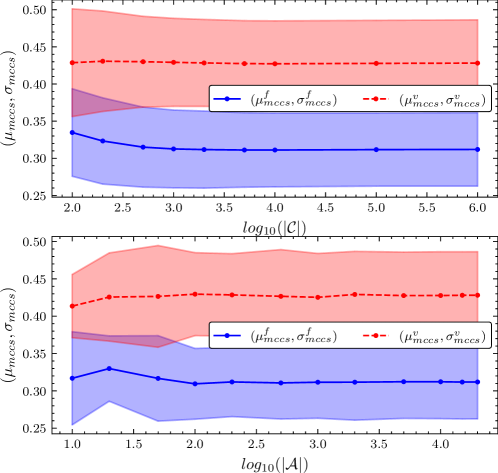
Figure 3. Justifying the sampling-efficiency of $(\mu_{\text{mccs}},\sigma_{\text{mccs}})$ w.r.t. $\log_{10}(|\mathcal{C}|)$ and $\log_{10}(|\mathcal{A}|)$ on the face generation task and vehicle generation task. $|\mathcal{A}|$ is the number of sampled anchor images. $|\mathcal{C}|$ is the number of sampled images. $\mathcal{A}\cap\mathcal{C}=\varnothing$. $(\mu_{\text{mccs}},\sigma_{\text{mccs}})$ can be reliably obtained at around $|\mathcal{A}|=10^{4}$ and $|\mathcal{C}|=10^{4}$.

Since white faces dominate both CelebAHQ and FFHQ, we combine the $30k$ images in CelebAHQ with the $70k$ images in FFHQ, discard the repeated identities, and randomly select $6k$ faces for each race in {White, Black Asian}. We called the resulting set Race-Identity-Calibrated-CelebAFFHQ (RIC). Next, we randomly pick one face for each race in the above set, repeat it 1,000 times, and add all repeated faces. This augmented set is called Race-Identity-Calibrated-CelebAFFHQ-aug (RIC-aug). Both RIC and RIC-aug have no inter-mode collapse since the number of different identities are equal across races. However, RIC-aug suffers from strong intra-mode collapse.

The two StyleGAN trained on RIC and RIC-aug at resolution of $128$ are denoted as $\mathcal{M}_{RIC}$ (FID=15.36) and $\mathcal{M}_{RIC-aug}$ (FID=15.93). Neither FID or the classification-based study (Santurkar et al., 2017) could reflect the intra-mode collapse in RIC-aug. Our proposed black-box diagnosis can detect intra-mode collapse by observing a huge gap between $\textit{MCCS}(\mathcal{I}_{w})=0.59$ and $\textit{MCCS}({\mathcal{I}_{w}^{\prime}})=0.81$, where $\mathcal{I}_{w}$ and $\mathcal{I}_{w}^{\prime}$ are the worst-case dense mode among the generated images of $\mathcal{M}_{RIC}$ and $\mathcal{M}_{RIC-aug}$ respectively.

StyleGAN Trained on CelebAHQ. Using $|\mathcal{A}|=10^{4}$ and $|\mathcal{C}|=10^{6}$ faces sampled from StyleGAN trained on CelebAHQ-$1024$, we run a “sanity check” on our proposed MCCS and show the results in Figure 4. The left figure $\mathcal{I}_{w}$, as an anchor face, is the worst-case dense mode in Eq.(9). The right figure $\mathcal{I}_{r}$ is a randomly selected anchor face. Both figures are surrounded with the top $80$ neighbors sorted by the distance function defined in Eq (4). $\mathcal{I}_{w}$ is clearly suffering from mode collapse since all its neighbor are almost identical to it. In contrast, the neighbors of $\mathcal{I}_{r}$ are quite diverse, though sharing some attribute-level similarities. Importantly, we have $\textit{MCCS}(\mathcal{I}_{w},\mathcal{C})=0.62$ $\gg$ $\textit{MCCS}(\mathcal{I}_{r},\mathcal{C})=0.35$, which agrees with the fact that $\mathcal{I}_{w}$ is the worst-case dense mode.

PacGAN Trained on CelebA. PacGAN (Lin et al., 2018) also reduces both inter- and intra-mode collapses at the same time. It can be represented in the form of “Pac(X)(m)”, where $X$ is the name of the backbone architecture (e.g., DCGAN (Radford et al., 2015)), and the integer $m$ refers to the number of samples packed together as input to the discriminator. We conduct our last experiment to run MCCS and see if it reflects an improvement. We adopt the SN-DCGAN (Miyato et al., 2018) architecture, set the number of packed sample $m$ to be $4$, and train the Pac(SN-DCGAN)(4) on CelebAHQ-128. The FID of SN-DCGAN and Pac(SN-DCGAN)(4) are $34.25$ and $28.12$, respectively. The $(\mu_{\text{mccs}},\sigma_{\text{mccs}})$ of SN-DCGAN and Pac(SN-DCGAN)(4) are $(0.62,0.18)$ and $(0.54,0.14)$ respectively. The $\textit{MCCS}(\mathcal{I}_{w})$ of SN-DCGAN and Pac(SN-DCGAN)(4) are are $0.84$ and $0.73$ respectively. Our proposed MCCS is able to reflect the improvement of PacGAN in both sample and population-level statistics.

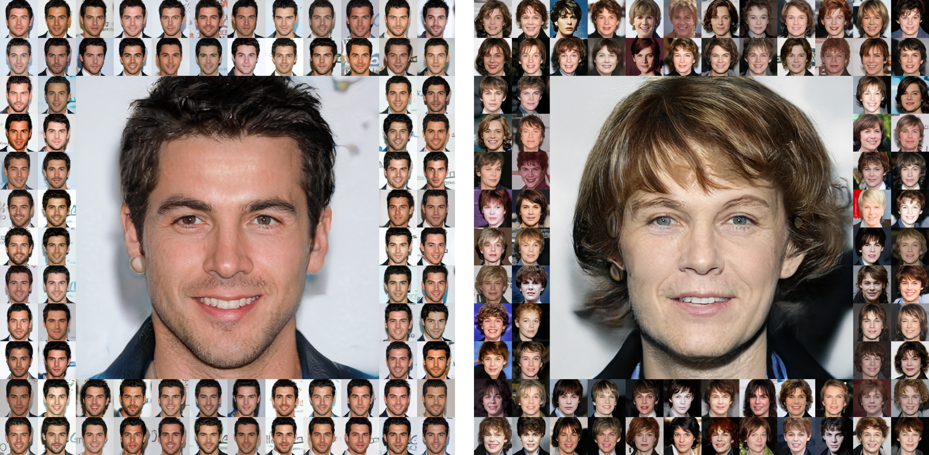
Figure 4. A “sanity check” of MCCS is run on StyleGAN trained with CelebAHQ. The left figure is $\mathcal{I}_{w}$ and the right figure is $\mathcal{I}_{r}$. Both figures are surrounded with the top $80$ neighbors sorted by distance function in Eq (4).

4.3. Black-box Diagnosis on Intra-Mode Collapse

4.3.1. Observation of Intra-Mode Collapse on State-Of-The-Art GANs

For StyleGAN (SGAN), StyleGAN2 (SGAN2), PGGAN, and BigGAN (BGAN), despite their observed diversity and high quality in generated images, we still find they are suffering from strong intra-mode collapse in Table 1. Note that PGGAN is trained on CelebAHQ-$1024$, StyleGAN on FFHQ-$1024$, StyleGAN2 on LSUN-Car-$1024$, and BigGAN on LSUN-Car-$1024$.

Table 1. Observation of intra-mode collapse on state-of-the-art GANs.

	SGAN	PGGAN	SGAN2	BGAN
$(\mu_{\text{mccs}},\sigma_{\text{mccs}})$	(0.41, 0.06)	(0.48, 0.07)	(0.31, 0.05)	(0.45, 0.07)
$\textit{MCCS}(\mathcal{I}_{w})$	0.64	0.72	0.56	0.69

4.3.2. Empirical Study on the Cause of Intra-Mode Collapse

We hypothesize multiple factors that may potentially lead to the observed dense mode (indicating intra-mode collapse) of face identity. We perform additional experiments, aiming to validate one by one. Despite the variance for the obtained sample-level and population-level statistics on MCCS, none of them was observed to cause the observed mode collapse. That implies the existence of some more intrinsic reason for the mode collapse in GAN, which we leave for future exploration.

Imbalance of Training Data? CelebAHQ is a highly imbalanced dataset: among its $30k$ high-resolution face images of $6,217$ different celebrities. It is natural to ask: would a balanced dataset alleviate the mode collapse? We turn to the Flickr-Faces-HQ Dataset (FFHQ), a high-quality human face dataset created in (Karras et al., 2018), consisting of $70k$ high-resolution images, without repeated identities. FFHQ dataset does not have an imbalance in facial attributes. To further eliminate the attribute-level imbalance, e.g., race, and gender, we combine the $30k$ images in CelebAHQ with the $70k$ images in FFHQ, and discard repeated images in identities. When selecting $6k$ faces for each race in {White, Black Asian}, we intentionally make the resulting set balanced in gender for each race. The resulting set is dubbed as Gender-Race-Identity-Calibrated-CelebAFFHQ (GRIC). As shown in Table 3, while the generation quality of StyleGAN trained on GRIC is still high, the intra-mode collapse persists and seems to be no less than StyleGAN on CelebAHQ and FFHQ. Therefore, imbalance of training data, regardless of at attribute-level or identity-level, does not cause intra-mode collapse.

Table 2. Empirical study on the cause of intra-mode collapse: imbalance of training data?

	CelebAHQ	FFHQ	GRIC
$(\mu_{\text{mccs}},\sigma_{\text{mccs}})$	(0.44, 0.08)	(0.41, 0.06)	(0.43, 0.06)
$\textit{MCCS}(\mathcal{I}_{w})$	0.67	0.64	0.62

Table 3. Empirical study on the cause of intra-mode collapse: model architecture differences?

		128	256	512	1024
SGAN	$(\mu_{\text{mccs}},\sigma_{\text{mccs}})$	(0.43,0.06)	(0.44,0.06)	(0.43,0.06)	(0.42,0.06)
	$\textit{MCCS}(\mathcal{I}_{w})$	0.64	0.63	0.65	0.65
PGGAN	$(\mu_{\text{mccs}},\sigma_{\text{mccs}})$	(0.52,0.08)	(0.51,0.09)	(0.53,0.08)	(0.52,0.08)
	$\textit{MCCS}(\mathcal{I}_{w})$	0.74	0.77	0.78	0.75

Randomness during Optimization? We repeat training StyleGAN on CelebAHQ-128 for 10 times, with different random initializations and mini-batching. We have $(\mu_{\text{mccs}},\sigma_{\text{mccs}})$ consistently around $(0.43,0.06)$. Despite little variances, the intra-mode collapse persists. We conclude that randomness during optimization is not the reason for intra-mode collapse.

Unfitting/Overfitting in Training? We train StyleGAN on CelebAHQ-128 again, and store model checkpoints at iteration $7707$ (FID = $7.67$, same hereinafter), $8307$ ($7.02$), $8908$ ($6.89$), $9508$ ($6.63$), $10108$ ($6.41$), and $12000$ ($6.32$). As the training iterations increases, $(\mu_{\text{mccs}},\sigma_{\text{mccs}})$ decreases from $(0.51,0.09)$ to $(0.43,0.06)$. Therefore, the intra-mode collapse persists, regardless of stopping the training earlier or later. We point out that unfittinng or overfitting is not the cause of intra-mode collapse.

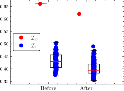
Figure 5. Reshaping Latent Space via Gaussian Mixture Models: mode collapse analysis of StyleGAN on CelebAHQ-128, before/after Gaussian mixture model-based reshaping.

Model Architecture Differences? Both StyleGAN and PGGAN progressively grow their architectures to generate images of different resolutions: $128$, $256$, $512$, and $1024$. Thus, we train StyleGAN and PGGAN on CelebAHQ-128, CelebAHQ-256, CelebAHQ-512, and CelebAHQ-1024, respectively. According to Table 3, varying the architectures does not eliminate the intra-mode collapse either. Thus, we empirically show that different model architectures do not lead to intra-mode collapse.

4.3.3. Diagnosis on Other Fine-Grained Image Generation

Flowers-$102$ consists of $102$ flower categories and is divided into $2,040$ images for training and $6,149$ for testing. CUB-$200$ has $200$ bird categories and is split into $5,994$ images for training and $5,794$ images for testing. We denote the identity descriptor for flower and bird as $F_{id}^{f}$ and $F_{id}^{b}$, respectively. Similarly, we denote the image generator for flower and bird as $G^{f}$ and $G^{b}$.

To obtain an accurate flower identity descriptor $F_{id}^{f}$, we adopt the EfficientNet (Tan and Le, 2019) and pretrain it on LifeCLEF2021 Plant Identification (Goëau et al., 2020; pla, [n.d.]; Goëau et al., 2016, 2017). Later on, we finetune it on a curated dataset that combines Jena Flowers 30 (Seeland et al., 2017), Flowers Recognition (flo, [n.d.]b), Flowers (flo, [n.d.]c), and Flowers-$17$ & Flowers-$102$ (flo, [n.d.]a). As an image generator, MSG-GAN (Karnewar and Wang, 2020) is trained on Flowers-$102$’s union of training and testing set, a total of $8,189$ images.

Table 4. Experiments on CUB-200 and Flowers-102

Dataset	Image Generator ($G$)	Identity Descriptor ($F_{id}$)	$(\mu_{\text{mccs}},\sigma_{\text{mccs}})$	$\textit{MCCS}(\mathcal{I}_{w})$
Flowers-$102$ (Nilsback and Zisserman, 2008)	MSG-GAN (Karnewar and Wang, 2020)	EfficientNet (Tan and Le, 2019)	$(0.69,0.12)$	$0.84$
CUB-$200$ (Welinder et al., 2010)	StackGAN-v2 (Zhang et al., 2018)	API-NET (Zhuang et al., 2020)	$(0.64,0.09)$	$0.86$

To obtain an accurate bird identity descriptor $F_{id}^{b}$, we adopt the API-NET (Zhuang et al., 2020) and pretrain it on the DongNiao International Birds $10000$ (DIB-$10$K) (Mei and Dong, 2020). Later on, we finetune it on a curated dataset that combines Bird265 (bir, [n.d.]) and NABirds (Van Horn et al., 2015). As an image generator, StackGAN-v2 is trained on CUB-$200$, a total of $11,788$ images.

According to Table 4, on the fine-grained image generation of birds and flowers, despite observed diversity and high quality in generated images, we can still spot strong intra-mode collapse.

4.4. Black-box Calibration on Intra-Mode Collapse

4.4.1. Reshaping Latent Space via Gaussian Mixture Models

Starting from a StyleGAN model $\mathcal{M}$ pre-trained on CelebAHQ-128, we aim at alleviating the collapse on the worst-case dense mode $\mathcal{I}_{w}$. We reshape the latent space of $\mathcal{M}$ via Gaussian mixture models to get the new model $\mathcal{M}^{\prime}$. We get the new worst-case dense mode $\mathcal{I}_{w}^{\prime}$ in $\mathcal{M}^{\prime}$. The $(\mu_{\text{mccs}},\sigma_{\text{mccs}})$ has decreased from $(0.43,0.06)$ to $(0.41,0.05)$. The $\textit{MCCS}(\mathcal{I}_{w})$ has also decreased from $0.66$ to $0.61$. Such an alleviation is achieved with an unnoticeable degradation of generation quality, with FID increasing from 5.93 ($\mathcal{M}$) to 5.95 ($\mathcal{M}^{\prime}$). As is shown in Figure 5, after applying the latent space reshaping, the intra-mode collapse has been alleviated, which are indicated by the large gap between $\mathcal{I}_{w}$ (before) and $\mathcal{I}_{w}^{\prime}$ (after), and the large gap between $\mathcal{I}_{r}$ (before) and $\mathcal{I}_{r}^{\prime}$ (after). For the sake of readability and visual quality, in each boxplot, only $100$ randomly chosen $\mathcal{I}_{r}$ are shown.

4.4.2. Reshaping Latent Space via Importance Sampling

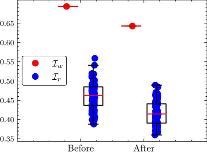
Figure 6. Reshaping Latent Space via Importance Sampling: mode collapse analysis of PGGAN on FFHQ-128, before/after importance sampling-based reshaping.

The experiment setting is mostly similar to the reshaping latent space via the Gaussian mixture models case, except that we are using PGGAN trained on FFHQ-128. We integrate importance sampling to the latent code generation stage. Given the dense mode $\mathcal{I}_{w}$, we can find the collection of latent codes from the top $10^{2}$ latent codes whose corresponding images have the smallest distances Eq.(4) to $\mathcal{I}_{w}$, among the $10^{6}$ random samples. We get the new worst-case dense mode $\mathcal{I}_{w}^{\prime}$ in $\mathcal{M}^{\prime}$. The $(\mu_{\text{mccs}},\sigma_{\text{mccs}})$ has decreased from $(0.46,0.07)$ to $(0.42,0.06)$. The $\textit{MCCS}(\mathcal{I}_{w})$ has also decreased from $0.69$ to $0.64$. The intra-mode collapse is again alleviated without sacrificing the visual quality of generated images, since FID only marginally increases from 9.43 ($\mathcal{M}$) to 9.46 ($\mathcal{M}^{\prime}$). As is shown in Figure 6, after applying the latent space reshaping, the intra-mode collapse has been alleviated, which are indicated by the large gap between $\mathcal{I}_{w}$ (before) and $\mathcal{I}_{w}^{\prime}$ (after), and the large gap between $\mathcal{I}_{r}$ (before) and $\mathcal{I}_{r}^{\prime}$ (after). For the sake of readability and visual quality, in each boxplot, only $100$ randomly chosen $\mathcal{I}_{r}$ are shown.

4.4.3. Why Calibrating the $\mathcal{I}_{w}$ Could Benefit the Calibration of Other Modes?

As is shown in Figure 7, we visualize the top $24$ modes with the largest number of neighbors within $0.25$ distance and found that they look very similar. Thus, we conclude that the dense region corresponding to $\mathcal{I}_{w}$ has occupied a considerably large portion in the number of supports in the GAN’s learned face identity distribution. Calibrating the worst-case mode $\mathcal{I}_{w}$ implicitly takes the entire dense region into account, since the entire dense region corresponding to the same face identity of $\mathcal{I}_{w}$.

5. Discussions and Future Work

This paper is intended as a pilot study on the intra-mode collapse issue of GANs, under a novel and hardly explored black-box setting. Using face and vehicle as study subjects, we quantify the general intra-mode collapse via statistical tools, discuss and verify possible causes, as well as propose two black-box calibration approaches for the first time to alleviate the mode collapse. Despite the preliminary success, the current study remains to be limited in many ways. First, there are inevitably prediction errors for the identity description on generated images, and even we have done our best to use the most accurate descriptors. Moreover, the fundamental causes of GAN mode collapse call for deeper understandings. We hope our work to draw more attention to studying both the intra-mode collapse problem and the new black-box setting.

Figure 7. Using the $10$ million face images sampled from a StyleGAN trained on CelebAHQ-$1024$, we visualize the top $24$ modes with largest number of neighbors within $0.25$ distance described by $F_{id}$ and found that they looks very similar. Calibrating the worst-case dense mode, which is the first mode shown here, implicitly takes the top $24$ modes dense modes into account.

References

- (1)
- bir ([n.d.]) [n.d.]. 265 Bird Species. https://www.kaggle.com/gpiosenka/100-bird-species.
- flo ([n.d.]a) [n.d.]a. Flowers-17 & Flowers-102. https://www.robots.ox.ac.uk/~vgg/data/flowers/.
- flo ([n.d.]b) [n.d.]b. Flowers Recognition. https://www.kaggle.com/alxmamaev/flowers-recognition.
- flo ([n.d.]c) [n.d.]c. Flowers Recognition. https://public.roboflow.com/classification/flowers/1.
- pla ([n.d.]) [n.d.]. PlantCLEF 2021: Cross-domain Plant Identification. https://www.imageclef.org/PlantCLEF2021.
- Amini et al. (2019) Alexander Amini, Ava Soleimany, Wilko Schwarting, Sangeeta Bhatia, and Daniela Rus. 2019. Uncovering and Mitigating Algorithmic Bias through Learned Latent Structure. (2019).
- Arjovsky et al. (2017) Martin Arjovsky, Soumith Chintala, and Léon Bottou. 2017. Wasserstein generative adversarial networks. In ICML.
- Arora et al. (2018) Sanjeev Arora, Andrej Risteski, and Yi Zhang. 2018. Do GANs learn the distribution? Some Theory and Empirics. In ICLR.
- Arora and Zhang (2017) Sanjeev Arora and Yi Zhang. 2017. Do gans actually learn the distribution? an empirical study. arXiv (2017).
- Azadi et al. (2018) Samaneh Azadi, Catherine Olsson, Trevor Darrell, Ian Goodfellow, and Augustus Odena. 2018. Discriminator rejection sampling. arXiv (2018).
- Barratt and Sharma (2018) Shane Barratt and Rishi Sharma. 2018. A note on the inception score. arXiv (2018).
- Bau et al. (2019) David Bau, Jun-Yan Zhu, Jonas Wulff, William Peebles, Hendrik Strobelt, Bolei Zhou, and Antonio Torralba. 2019. Seeing what a gan cannot generate. In ICCV.
- Borji (2019) Ali Borji. 2019. Pros and cons of gan evaluation measures. Computer Vision and Image Understanding (2019).
- Bowles et al. (2018) Christopher Bowles, Roger Gunn, Alexander Hammers, and Daniel Rueckert. 2018. GANsfer Learning: Combining labelled and unlabelled data for GAN based data augmentation. arXiv (2018).
- Brock et al. (2018) Andrew Brock, Jeff Donahue, and Karen Simonyan. 2018. Large scale gan training for high fidelity natural image synthesis. arXiv (2018).
- Che et al. (2016) Tong Che, Yanran Li, Athul Paul Jacob, Yoshua Bengio, and Wenjie Li. 2016. Mode regularized generative adversarial networks. arXiv (2016).
- Deng et al. (2019a) Jiankang Deng, Jia Guo, Xue Niannan, and Stefanos Zafeiriou. 2019a. ArcFace: Additive Angular Margin Loss for Deep Face Recognition. In CVPR.
- Deng et al. (2019b) Jiankang Deng, Jia Guo, Zhou Yuxiang, Jinke Yu, Irene Kotsia, and Stefanos Zafeiriou. 2019b. RetinaFace: Single-stage Dense Face Localisation in the Wild. In arxiv.
- Deng et al. (2018) Jiankang Deng, Anastasios Roussos, Grigorios Chrysos, Evangelos Ververas, Irene Kotsia, Jie Shen, and Stefanos Zafeiriou. 2018. The Menpo benchmark for multi-pose 2D and 3D facial landmark localisation and tracking. IJCV (2018).
- Durugkar et al. (2016) Ishan Durugkar, Ian Gemp, and Sridhar Mahadevan. 2016. Generative multi-adversarial networks. arXiv (2016).
- Filipovych et al. (2011) Roman Filipovych, Christos Davatzikos, Alzheimer’s Disease Neuroimaging Initiative, et al. 2011. Semi-supervised pattern classification of medical images: application to mild cognitive impairment (MCI). NeuroImage (2011).
- Ghosh et al. (2018) Arnab Ghosh, Viveka Kulharia, Vinay P Namboodiri, Philip HS Torr, and Puneet K Dokania. 2018. Multi-agent diverse generative adversarial networks. In CVPR.
- Goëau et al. (2016) Hervé Goëau, Pierre Bonnet, and Alexis Joly. 2016. Plant identification in an open-world (lifeclef 2016). In CLEF: Conference and Labs of the Evaluation Forum.
- Goëau et al. (2017) Hervé Goëau, Pierre Bonnet, and Alexis Joly. 2017. Plant identification based on noisy web data: the amazing performance of deep learning (LifeCLEF 2017). In CLEF: Conference and Labs of the Evaluation Forum.
- Goëau et al. (2020) Hervé Goëau, Pierre Bonnet, and Alexis Joly. 2020. Overview of lifeclef plant identification task 2020. In CLEF 2020-Conference and labs of the Evaluation Forum.
- Gong et al. (2019) Xinyu Gong, Shiyu Chang, Yifan Jiang, and Zhangyang Wang. 2019. Autogan: Neural architecture search for generative adversarial networks. In ICCV.
- Goodfellow (2016) Ian Goodfellow. 2016. NIPS 2016 tutorial: Generative adversarial networks. arXiv (2016).
- Goodfellow et al. (2014) Ian Goodfellow, Jean Pouget-Abadie, Mehdi Mirza, Bing Xu, David Warde-Farley, Sherjil Ozair, Aaron Courville, and Yoshua Bengio. 2014. Generative adversarial nets. In NeurIPS.
- Guo et al. (2018) Jia Guo, Jiankang Deng, Niannan Xue, and Stefanos Zafeiriou. 2018. Stacked Dense U-Nets with Dual Transformers for Robust Face Alignment. In BMVC.
- Heusel et al. (2017) Martin Heusel, Hubert Ramsauer, Thomas Unterthiner, Bernhard Nessler, and Sepp Hochreiter. 2017. Gans trained by a two time-scale update rule converge to a local nash equilibrium. In NeurIPS.
- Holstein et al. (2018) Kenneth Holstein, Jennifer Wortman Vaughan, Hal Daumé III, Miro Dudík, and Hanna Wallach. 2018. Improving fairness in machine learning systems: What do industry practitioners need? arXiv (2018).
- Huang et al. (2018) He Huang, Philip S Yu, and Changhu Wang. 2018. An introduction to image synthesis with generative adversarial nets. arXiv preprint arXiv:1803.04469 (2018).
- Jiang et al. (2021a) Yifan Jiang, Shiyu Chang, and Zhangyang Wang. 2021a. Transgan: Two transformers can make one strong gan. arXiv (2021).
- Jiang et al. (2021b) Yifan Jiang, Xinyu Gong, Ding Liu, Yu Cheng, Chen Fang, Xiaohui Shen, Jianchao Yang, Pan Zhou, and Zhangyang Wang. 2021b. Enlightengan: Deep light enhancement without paired supervision. TIP (2021).
- Karnewar and Wang (2020) Animesh Karnewar and Oliver Wang. 2020. Msg-gan: Multi-scale gradients for generative adversarial networks. In CVPR.
- Karras et al. (2017) Tero Karras, Timo Aila, Samuli Laine, and Jaakko Lehtinen. 2017. Progressive growing of gans for improved quality, stability, and variation. arXiv (2017).
- Karras et al. (2018) Tero Karras, Samuli Laine, and Timo Aila. 2018. A style-based generator architecture for generative adversarial networks. arXiv (2018).
- Karras et al. (2019) Tero Karras, Samuli Laine, Miika Aittala, Janne Hellsten, Jaakko Lehtinen, and Timo Aila. 2019. Analyzing and improving the image quality of stylegan. arXiv (2019).
- Kupyn et al. (2019) Orest Kupyn, Tetiana Martyniuk, Junru Wu, and Zhangyang Wang. 2019. Deblurgan-v2: Deblurring (orders-of-magnitude) faster and better. In ICCV.
- Lin et al. (2018) Zinan Lin, Ashish Khetan, Giulia Fanti, and Sewoong Oh. 2018. Pacgan: The power of two samples in generative adversarial networks. In NeurIPS.
- Liu and Tuzel (2016) Ming-Yu Liu and Oncel Tuzel. 2016. Coupled generative adversarial networks. In NeurIPS.
- Liu et al. (2019) Shuangting Liu, Jiaqi Zhang, Yuxin Chen, Yifan Liu, Zengchang Qin, and Tao Wan. 2019. Pixel Level Data Augmentation for Semantic Image Segmentation using Generative Adversarial Networks. In ICASSP.
- Liu et al. (2018) Xiaobin Liu, Shiliang Zhang, Qingming Huang, and Wen Gao. 2018. RAM: A Region-Aware Deep Model for Vehicle Re-Identification. In ICME.
- Mao et al. (2017) Xudong Mao, Qing Li, Haoran Xie, Raymond YK Lau, Zhen Wang, and Stephen Paul Smolley. 2017. Least squares generative adversarial networks. In ICCV.
- Mei and Dong (2020) Jian Mei and Hao Dong. 2020. The DongNiao International Birds 10000 Dataset. arXiv (2020).
- Metz et al. (2016) Luke Metz, Ben Poole, David Pfau, and Jascha Sohl-Dickstein. 2016. Unrolled Generative Adversarial Networks.
- Miyato et al. (2018) Takeru Miyato, Toshiki Kataoka, Masanori Koyama, and Yuichi Yoshida. 2018. Spectral Normalization for Generative Adversarial Networks. In ICLR.
- Nilsback and Zisserman (2008) Maria-Elena Nilsback and Andrew Zisserman. 2008. Automated flower classification over a large number of classes. In 2008 Sixth Indian Conference on Computer Vision, Graphics & Image Processing. IEEE.
- Radford et al. (2015) Alec Radford, Luke Metz, and Soumith Chintala. 2015. Unsupervised representation learning with deep convolutional generative adversarial networks. arXiv (2015).
- Salimans et al. (2016) Tim Salimans, Ian Goodfellow, Wojciech Zaremba, Vicki Cheung, Alec Radford, and Xi Chen. 2016. Improved techniques for training gans. In NeurIPS.
- Santurkar et al. (2017) Shibani Santurkar, Ludwig Schmidt, and Aleksander Mądry. 2017. A classification-based study of covariate shift in gan distributions. arXiv (2017).
- Sattigeri et al. (2018) Prasanna Sattigeri, Samuel C Hoffman, Vijil Chenthamarakshan, and Kush R Varshney. 2018. Fairness gan. arXiv (2018).
- Savchenko (2019) Andrey V Savchenko. 2019. Efficient facial representations for age, gender and identity recognition in organizing photo albums using multi-output ConvNet. PeerJ Computer Science (2019).
- Seeland et al. (2017) Marco Seeland, Michael Rzanny, Nedal Alaqraa, Jana Wäldchen, and Patrick Mäder. 2017. Jena Flowers 30 Dataset. https://doi.org/10.7910/DVN/QDHYST
- Srivastava et al. (2017) Akash Srivastava, Lazar Valkov, Chris Russell, Michael U Gutmann, and Charles Sutton. 2017. Veegan: Reducing mode collapse in gans using implicit variational learning. In NeurIPS.
- Sutskever et al. (2015) Ilya Sutskever, Rafal Jozefowicz, Karol Gregor, Danilo Rezende, Tim Lillicrap, and Oriol Vinyals. 2015. Towards principled unsupervised learning. arXiv (2015).
- Tan and Le (2019) Mingxing Tan and Quoc Le. 2019. Efficientnet: Rethinking model scaling for convolutional neural networks. In ICML. PMLR.
- Turner et al. (2018) Ryan Turner, Jane Hung, Yunus Saatci, and Jason Yosinski. 2018. Metropolis-hastings generative adversarial networks. arXiv (2018).
- Uplavikar et al. (2019) Pritish M Uplavikar, Zhenyu Wu, and Zhangyang Wang. 2019. All-in-One Underwater Image Enhancement Using Domain-Adversarial Learning.. In CVPR Workshops.
- Van Horn et al. (2015) Grant Van Horn, Steve Branson, Ryan Farrell, Scott Haber, Jessie Barry, Panos Ipeirotis, Pietro Perona, and Serge Belongie. 2015. Building a bird recognition app and large scale dataset with citizen scientists: The fine print in fine-grained dataset collection. In CVPR.
- Wang et al. (2020b) Angelina Wang, Arvind Narayanan, and Olga Russakovsky. 2020b. REVISE: A Tool for Measuring and Mitigating Bias in Visual Datasets. In ECCV.
- Wang et al. (2020a) Haotao Wang, Shupeng Gui, Haichuan Yang, Ji Liu, and Zhangyang Wang. 2020a. GAN Slimming: All-in-One GAN Compression by A Unified Optimization Framework. In ECCV. Springer.
- Webster et al. (2019) Ryan Webster, Julien Rabin, Loic Simon, and Frederic Jurie. 2019. Detecting Overfitting of Deep Generative Networks via Latent Recovery. arXiv (2019).
- Welinder et al. (2010) P. Welinder, S. Branson, T. Mita, C. Wah, F. Schroff, S. Belongie, and P. Perona. 2010. Caltech-UCSD Birds 200. Technical Report CNS-TR-2010-001. California Institute of Technology.
- Wu et al. (2020a) Zhenyu Wu, Duc Hoang, Shih-Yao Lin, Yusheng Xie, Liangjian Chen, Yen-Yu Lin, Zhangyang Wang, and Wei Fan. 2020a. MM-Hand: 3D-Aware Multi-Modal Guided Hand Generation for 3D Hand Pose Synthesis. In ACMMM.
- Wu et al. (2019) Zhenyu Wu, Karthik Suresh, Priya Narayanan, Hongyu Xu, Heesung Kwon, and Zhangyang Wang. 2019. Delving into robust object detection from unmanned aerial vehicles: A deep nuisance disentanglement approach. In ICCV.
- Wu et al. (2020b) Zhenyu Wu, Haotao Wang, Zhaowen Wang, Hailin Jin, and Zhangyang Wang. 2020b. Privacy-Preserving Deep Action Recognition: An Adversarial Learning Framework and A New Dataset. TPAMI (2020).
- Wu et al. (2018) Zhenyu Wu, Zhangyang Wang, Zhaowen Wang, and Hailin Jin. 2018. Towards privacy-preserving visual recognition via adversarial training: A pilot study. In Proceedings of the European Conference on Computer Vision (ECCV).
- Xie et al. (2018) Liyang Xie, Kaixiang Lin, Shu Wang, Fei Wang, and Jiayu Zhou. 2018. Differentially private generative adversarial network. arXiv (2018).
- Xu et al. (2018) Depeng Xu, Shuhan Yuan, Lu Zhang, and Xintao Wu. 2018. Fairgan: Fairness-aware generative adversarial networks. In ICBD.
- Yang et al. (2021) Shuai Yang, Zhangyang Wang, and Jiaying Liu. 2021. Shape-Matching GAN++: Scale Controllable Dynamic Artistic Text Style Transfer. TPAMI (2021).
- Yang et al. (2020) Shuai Yang, Zhangyang Wang, Jiaying Liu, and Zongming Guo. 2020. Deep plastic surgery: Robust and controllable image editing with human-drawn sketches. In European Conference on Computer Vision. Springer, 601–617.
- Yang et al. (2019) Shuai Yang, Zhangyang Wang, Zhaowen Wang, Ning Xu, Jiaying Liu, and Zongming Guo. 2019. Controllable artistic text style transfer via shape-matching gan. In ICCV.
- Yu et al. (2015) Fisher Yu, Ari Seff, Yinda Zhang, Shuran Song, Thomas Funkhouser, and Jianxiong Xiao. 2015. Lsun: Construction of a large-scale image dataset using deep learning with humans in the loop. arXiv (2015).
- Zhang et al. (2018) Han Zhang, Tao Xu, Hongsheng Li, Shaoting Zhang, Xiaogang Wang, Xiaolei Huang, and Dimitris N Metaxas. 2018. Stackgan++: Realistic image synthesis with stacked generative adversarial networks. TPMAI (2018).
- Zhang et al. (2019) Xiaofeng Zhang, Zhangyang Wang, Dong Liu, and Qing Ling. 2019. DADA: Deep adversarial data augmentation for extremely low data regime classification. In ICASSP.
- Zheng et al. (2019) Aihua Zheng, Xianmin Lin, Chenglong Li, Ran He, and Jin Tang. 2019. Attributes guided feature learning for vehicle re-identification. arXiv (2019).
- Zheng et al. (2020) Yuli Zheng, Zhenyu Wu, Ye Yuan, Tianlong Chen, and Zhangyang Wang. 2020. PCAL: A Privacy-preserving Intelligent Credit Risk Modeling Framework Based on Adversarial Learning. arXiv (2020).
- Zhou et al. (2017) Zhiming Zhou, Weinan Zhang, and Jun Wang. 2017. Inception score, label smoothing, gradient vanishing and-log (d (x)) alternative. arXiv (2017).
- Zhuang et al. (2020) Peiqin Zhuang, Yali Wang, and Yu Qiao. 2020. Learning attentive pairwise interaction for fine-grained classification. In AAAI.