Entanglement entropy of inhomogeneous XX spin chains with algebraic interactions

Abstract

We introduce a family of inhomogeneous XX spin chains whose squared couplings are a polynomial of degree at most four in the site index. We show how to obtain an asymptotic approximation for the Rényi entanglement entropy of all such chains in a constant magnetic field at half filling by exploiting their connection with the conformal field theory of a massless Dirac fermion in a suitably curved static background. We study the above approximation for three particular chains in the family, two of them related to well-known quasi-exactly solvable quantum models on the line and the third one to classical Krawtchouk polynomials, finding an excellent agreement with the exact value obtained numerically when the Rényi parameter $\alpha$ is less than one. When $\alpha\geqslant 1$ we find parity oscillations, as expected from the homogeneous case, and show that they are very accurately reproduced by a modification of the Fagotti–Calabrese formula. We have also analyzed the asymptotic behavior of the Rényi entanglement entropy in the non-standard situation of arbitrary filling and/or inhomogeneous magnetic field. Our numerical results show that in this case a block of spins at each end of the chain becomes disentangled from the rest. Moreover, the asymptotic approximation for the case of half filling and constant magnetic field, when suitably rescaled to the region of non-vanishing entropy, provides a rough approximation to the entanglement entropy also in this general case.

1 Introduction

The entanglement entropy of spin chains of XX type —or, equivalently, systems of free spinless fermions with nearest-neighbors hoppings— has been intensively studied since the seminal work of Jin and Korepin JK04 for the homogeneous chain. Indeed, the bipartite entanglement entropy of one-dimensional models is a convenient indicator of their criticality. The reason is that in their critical phase these models are effectively described at low energies by a ($1+1$)-dimensional conformal field theory (CFT), whose entanglement entropy has been shown to scale logarithmically with the block size $L$ CC04JSTAT ; CC09 . In fact, a fundamental property of all XX-type spin chains is the fact that their entanglement entropy can be expressed in terms of the eigenvalues of a (truncated) correlation matrix. In the homogeneous case this matrix is Toeplitz (for closed chains) or Toeplitz$+$Hankel (for open ones), which makes it possible to apply proved instances of the (generalized) Fisher–Hartwig conjecture FH68 ; Ba79 ; DIK11 to rigorously derive the leading asymptotic behavior of the entanglement entropy. In this way it was shown that the Rényi entanglement entropy $S_{\alpha}$ of the homogeneous XX spin chain is asymptotically proportional to $\log L$ in the open, closed and (semi)infinite cases JK04 ; CE10 , even for subsystems of more than one block CH09 ; CCT09 ; ATC10 ; FC10 ; CFGT17 . Moreover, the coefficient of $\log L$ in the asymptotic formula for $S_{\alpha}$ confirms that this model has central charge $c=1$, as expected.

In fact, corrections to the logarithmic behavior of $S_{\alpha}$ in the limit of large $L$ were exhaustively analyzed by Calabrese and Essler for the closed homogeneous XX chain CE10 , and by Fagotti and Calabrese for the open one FC11 . For $\alpha>1$, or $\alpha\geqslant 1$ in the open case, these terms present an oscillatory behavior which is particularly simple in the open case. Indeed, in this case the leading order correction is proportional to $\sin((2L+1)k_{F})L^{-1/\alpha}$, where $k_{F}$ is the Fermi momentum. Moreover, it is argued in Ref. FC11 (and earlier in CCEN10 ) that this correction —more precisely, the exponent of $L$ in the formula for the amplitude— encodes additional information about the underlying CFT beyond the central charge.

The situation is less straightforward in the non-homogeneous case, since the correlation matrix is in general neither Toeplitz nor Toeplitz$+$Hankel. However, at half filling and constant magnetic field, the leading behavior of the bipartite entanglement entropy can be derived through the technique first used in Ref. RDRCS17 to study the rainbow chain VRL10 . The main idea is that with these assumptions the chain’s continuum limit yields the CFT of a massless Dirac fermion in a static curved ($1+1$)-dimensional spacetime, whose metric’s conformal factor is proportional to the square of (the continuum limit of) the hopping amplitude. This suggests that in the thermodynamic limit the leading asymptotic behavior of $S_{\alpha}$ can be obtained from the formula for the homogeneous case replacing the chain’s and block’s lengths by their conformal versions DSVC17 . This was actually shown to be the case for the rainbow chain in Ref. TRS18 , and more recently for several other inhomogeneous XX chains in Refs. FG20 ; MSR21 . We stress, however, that to the best of our knowledge the latter results only hold in the case of half filling and constant magnetic field. Moreover, the method just outlined has only been applied to the leading term in the asymptotic formula for $S_{\alpha}$, without addressing the behavior of the subleading corrections.

Another fundamental property of XX spin chains is their close connection with classical orthogonal polynomials. Indeed, the chain’s single-particle Hamiltonian is represented in the position basis by a real tridiagonal symmetric matrix (the so-called hopping matrix), whose elements can in turn be used to define a three-term recursion relation determining a finite orthogonal polynomial system (OPS) $\{P_{n}\}_{n=0}^{N}$, where $N$ is the number of spins. This establishes a one-to-one correspondence between XX spin chains and OPSs, that can be used to derive in a simple way many of the chain’s properties. Indeed, the single-particle energies are the roots of the critical polynomial $P_{N}$, and the correlation matrix elements can be computed in closed form (without need of numerical diagonalization) in terms of the polynomials in the OPS evaluated at the latter energies. This turns out to be more efficient than brute force diagonalization of the matrix of the single-particle Hamiltonian as the number of spins grows. This connection has also been exploited in Ref. CNV19 to construct in some cases a tridiagonal matrix commuting with the hopping matrix of the entanglement Hamiltonian, which can be used to improve the numerical accuracy of the eigenvalues of the latter matrix and hence of the entanglement entropy.

A key property shared by the chains studied in Ref. CNV19 is the fact that the square of the interaction strength $J_{n}$ is a polynomial of degree at most four in the site index $n$. This property is very natural from the point of view of the associated orthogonal polynomial family, since $-J_{n-1}^{2}$ coincides with the coefficient of $P_{n-1}$ in the recursion relation for $P_{n+1}$. In fact, the latter property also holds for the inhomogeneous XX chains related to one-dimensional quasi-exactly solvable (QES) models Tu88 ; Sh89 ; ST89 ; Us94 introduced in Ref. FG20 . We shall show in this work that for all XX spin chains for which $J_{n}^{2}$ is a polynomial of degree up to four in $n$ it is possible to evaluate in closed form the leading asymptotic approximation to the ground-state entanglement entropy (at half filling and in a constant magnetic field) by the procedure introduced in Ref. RDRCS17 . This in done essentially by reducing a suitable elliptic integral to Legendre canonical form, a procedure which depends on the root pattern of $J_{n}^{2}$.

We shall analyze in some detail three inhomogeneous XX chains with interactions $J_{n}$ of the algebraic form described in the previous paragraph (algebraic interactions, for short). Two of these chains arise from well-known QES potentials, namely the sextic oscillator and the Lamé periodic potential, while the third one, introduced in Ref. CNV19 , is associated to the Krawtchouk discrete orthogonal polynomial family. We first of all check that the leading term in the asymptotic approximation to the entanglement entropy obtained through the related massless Dirac fermion CFT in a suitably curved background is in excellent agreement with the numerical results in the standard scenario of constant magnetic field and half filling. Moreover, for the sextic and Krawtchouk chains at half filling and in a constant magnetic field we have found strong numerical evidence that the subleading (constant) term in the asymptotic expansion of the entanglement entropy coincides with its counterpart for the homogeneous XX chain for $N$ large enough. To the best of our knowledge, this remarkable coincidence had not been previously noticed in the literature. We stress in this regard that the connection of the models under study with families of orthogonal polynomials makes it possible to determine the eigenvalues and eigenvectors of the single-particle Hamiltonian in a numerically efficient way when the number of spins is very large. Our numerical calculations also indicate that when $\alpha\geqslant 1$ the Rényi entanglement entropy $S_{\alpha}$ features parity oscillations which become more marked as $\alpha$ increases, as in the homogeneous case. Remarkably, these oscillations are reproduced with great precision by the heuristic formula proposed by Fagotti and Calabrese for the homogeneous XX chain, replacing the lengths of the block and the whole chain by their values computed with the metric of the ambient space of the associated CFT. More precisely, this formula depends only on two free parameters, whose fitted values are very close to the theoretical ones for the homogeneous XX chain. This underscores the essential similarity of the homogeneous and inhomogeneous cases, and the universality of Fagotti and Calabrese’s formula for this class of models.

All of the above results have been obtained under the standard assumptions of constant magnetic field and half filling, for which the connection with the massless Dirac fermion CFT has a theoretical justification via the continuum limit. In this work we have also analyzed the non-standard situations of arbitrary filling and/or inhomogeneous magnetic field, which to the best of our knowledge have not been addressed in the literature. Our numerical calculations clearly indicate that the new feature in both of these scenarios is the vanishing of the entanglement entropy when the length of the block is small or close to the chain’s length. In other words, the first few and last spins become disentangled from the rest of the chain. As a consequence, the (leading) asymptotic approximation to the entanglement entropy derived from the associated CFT cannot be expected to hold in this case. Remarkably, we have checked that this approximation roughly reproduces the average behavior of $S_{\alpha}$ if suitably scaled to the region of non-vanishing entropy. On the other hand, the oscillations of $S_{\alpha}$ in these non-standard cases are found to be much more complex than in the usual situation of half filling and constant magnetic field, and in particular are not well reproduced by the conformally modified version of the Fagotti–Calabrese formula.

The paper is organized as follows. In Section 2 we briefly review the connection between inhomogeneous XX spin chains and free fermion systems, and recall how the latter models can be exactly diagonalized. Likewise, in Section 3 we explain how these models are related to a finite orthogonal polynomial family through its three-term recursion relation, and how to exploit this connection to diagonalize the single-particle Hamiltonian. In Section 4 we summarize the main results on the bipartite entanglement entropy of spin chains used throughout the paper. In particular, we review some known results about the asymptotic behavior of the entanglement entropy of the homogeneous XX chain as the number of spins tends to infinity, and briefly outline their recent extension to the non-homogeneous case at half filling in a constant magnetic field. In Section 5 we present a class of inhomogeneous XX spin chains with algebraic interactions for which it is possible to compute in closed form an asymptotic approximation to the block entanglement entropy by the procedure explained above. The next three sections are devoted to the detailed analysis of three models in the previous family, associated to the QES sextic oscillator Hamiltonian (Section 6), the classical Krawtchouk polynomials (Section 7) and the periodic Lamé potential (Section 8). In Section 9 we present our conclusions and discuss several lines for future research. The paper ends with a technical appendix explaining how to reduce to Legendre canonical form the elliptic integral appearing in the asymptotic formula for the entanglement entropy.

2 Inhomogeneous XX spin chains and free fermion systems

The Hamiltonian of an inhomogeneous XX spin chain with interactions $J_{n}$ in an external magnetic field $B_{n}$ can be taken as

$$H=\frac{1}{2}\sum_{n=0}^{N-2}J_{n}(\sigma_{n}^{x}\sigma_{n+1}^{x}+\sigma_{n}^{y}\sigma_{n+1}^{y})+\frac{1}{2}\sum_{n=0}^{N-1}B_{n}(1-\sigma_{n}^{z})\,,$$ (1)

where $N$ is the number of sites and $\sigma_{n}^{\alpha}$ (with $\alpha=x,y,z$) denotes the Pauli matrix $\sigma^{\alpha}$ acting on the $n$-th site. In what follows we shall assume that the interaction strengths $J_{n}$ do not vanish. As remarked in Ref. FG20 , the model with $J_{n}$ replaced by $\varepsilon_{n}J_{n}$, where $\varepsilon_{n}\in\{\pm 1\}$ is a site-dependent sign, is unitarily equivalent to the original one. Hence we can take all the $J_{n}$’s to be positive without loss of generality.

It is well known that the Jordan–Wigner transformation

$$c_{n}=\prod_{k=0}^{n-1}\sigma_{k}^{z}\cdot\sigma_{n}^{+}\,,\qquad 0\leqslant n\leqslant N-1\,,$$ (2)

where $\sigma^{\pm}_{n}:=(\sigma^{x}_{n}\pm\mathrm{i}\sigma^{y}_{n})/2$, maps the Hamiltonian (1) into that of a system of $N$ hopping spinless fermions,

$$H=\sum_{n=0}^{N-2}J_{n}(c^{\dagger}_{n}c_{n+1}+c^{\dagger}_{n+1}c_{n})+\sum_{n=0}^{N-1}B_{n}c^{\dagger}_{n}c_{n}\,.$$ (3)

Here $c^{\dagger}_{n}$ (resp. $c_{n}$) is the operator creating (resp. destroying) a fermion at site $n$, and the coefficients $J_{n}$ and $B_{n}$ respectively represent the hopping amplitude and the chemical potential of the fermions. In what follows we shall mainly deal with the free fermion system (3), our results being easily translated to its spin chain equivalent (1).

In the homogeneous case (i.e., when $J_{n}$ and $B_{n}$ are site independent), the Hamiltonian (3) commutes with the translation operator along the chain sites and is thus diagonal in momentum space. In the non-homogeneous case this symmetry is lost, but the Hamiltonian can still be diagonalized by introducing suitable modes. More precisely, let

$$\mathsf{H}=(H_{nm})_{n,m=0}^{N-1}\,,\qquad\text{with}\quad H_{nm}=\langle n|H|m\rangle=J_{n}\delta_{m,n+1}+J_{n-1}\delta_{m,n-1}+B_{n}\delta_{nm}\,,$$ (4)

denote the matrix of the restriction of $H$ to the single-particle sector with respect to the position basis

$$\Big{\{}|n\rangle:=c^{\dagger}_{n}|\mathrm{vac}\rangle\mid 0\leqslant n\leqslant N-1\Big{\}}\,,$$

where $|\mathrm{vac}\rangle$ is the fermionic vacuum. Since the hopping matrix $\mathsf{H}$ is real and symmetric, it can be diagonalized by a real orthogonal matrix $\Phi=(\Phi_{nk})_{n,k=0}^{N-1}$, namely

$$\Phi^{T}\mathsf{H}\Phi=\operatorname{diag}(\varepsilon_{0},\dots,\varepsilon_{N-1})\,,$$ (5)

where $\varepsilon_{0}<\dots<\varepsilon_{N-1}\in{\mathbb{R}}$ are the eigenvalues of $\mathsf{H}$. Note that, since $\mathsf{H}$ is tridiagonal with nonzero off-diagonal entries, all its eigenvalues are simple. Let us then define a new set of fermionic operators through the relation

$$\tilde{c}_{k}:=\sum_{n=0}^{N-1}\Phi_{nk}c_{n}\,,\qquad 0\leqslant k\leqslant N-1,$$ (6)

which satisfy the canonical anticommutation relations (CAR) on account of the unitary (real orthogonal) character of $\Phi$. It is easily shown that the Hamiltonian (3) can be written as

$$H=\sum_{k=0}^{N-1}\varepsilon_{k}\tilde{c}^{\dagger}_{k}\tilde{c}_{k}\,,$$ (7)

and is thus diagonal in the basis consisting of the states

$$\tilde{c}^{\dagger}_{k_{0}}\cdots\tilde{c}_{k_{l}}^{\dagger}|\mathrm{vac}\rangle\,,\qquad 0\leqslant k_{0}<\cdots<k_{l}\leqslant N-1\,,$$ (8)

whose corresponding energy is given by

$$E(k_{0},\dots,k_{l})=\sum_{j=0}^{l}\varepsilon_{k_{j}}\,.$$ (9)

In particular, the one-particle eigenstates $\tilde{c}^{\dagger}_{k}|\mathrm{vac}\rangle$ (with $0\leqslant k\leqslant N-1$) represent single-fermion excitation modes with energy $\varepsilon_{k}$.

The case in which the magnetic field $B_{n}$ vanishes for all $n$ deserves special attention. Indeed, in this case $H$ is equivalent to $-H$ under the unitary transformation $c_{n}\mapsto(-1)^{n}c_{n}$ (which obviously preserves the CAR), so that the spectrum is symmetric about zero:

$$\varepsilon_{N-k-1}=-\varepsilon_{k}\,,\qquad 0\leqslant k\leqslant N-1\,.$$

This implies that the system possesses particle-hole symmetry, since if $n_{1}^{\prime}<\cdots<n_{N-k-1}^{\prime}$ with $\{n_{1}^{\prime},\dots,n_{N-k-1}^{\prime}\}\cup\{n_{1},\dots,n_{k}\}=\{0,\dots,N-1\}$ we have

$$E(n_{1}^{\prime},\dots,n_{N-k-1}^{\prime})=\sum_{i=0}^{N-1}\varepsilon_{i}-E(n_{1},\dots,n_{k})=-E(n_{1},\dots,n_{k})\,.$$

Moreover, from the equivalence of $H$ to $-H$ under $c_{n}\mapsto(-1)^{n}c_{n}$ we immediately obtain the relation

$$\Phi_{n,N-k-1}=(-1)^{n}\Phi_{nk}$$ (10)

up to an $n$-independent sign. Thus when $N$ is even the ground state is the half-filled state

$$\tilde{c}^{\dagger}_{0}\cdots\tilde{c}^{\dagger}_{N/2-1}|\mathrm{vac}\rangle\,,$$ (11)

with Fermi momentum $\pi/2$ and energy

$$E_{0}:=\sum_{k=0}^{\mathchoice{\hbox to0.0pt{\hss$\displaystyle{N/2-1}$\hss}}{\hbox to0.0pt{\hss$\textstyle{N/2-1}$\hss}}{\hbox to0.0pt{\hss$\scriptstyle{N/2-1}$\hss}}{\hbox to0.0pt{\hss$\scriptscriptstyle{N/2-1}$\hss}}}\varepsilon_{k}\,.$$ (12)

(When $N$ is odd the ground state is doubly degenerate, since the zero energy mode does not change the total energy.)

3 Orthogonal polynomials

As explained in the previous section, the diagonalization of the full Hamiltonian (3) of a free fermion system is achieved by diagonalizing the hopping matrix $\mathsf{H}$ in Eq. (4). Since the latter matrix is tridiagonal, it can be used to define a finite orthogonal polynomial system $\{\phi_{n}(E)\}_{n=0}^{N}$ through the three-term recursion relation

$$E\phi_{n}(E)=J_{n}\phi_{n+1}(E)+B_{n}\phi_{n}(E)+J_{n-1}\phi_{n-1}(E)\,,\qquad 0\leqslant n\leqslant N-1$$ (13)

(with $\phi_{-1}:=0$). It is easily shown that the polynomial $\phi_{N}(E)$ is proportional to the characteristic polynomial of $\mathsf{H}$, and that the matrix elements of $\Phi$ can be taken as $\Phi_{nk}=\phi_{n}(\varepsilon_{k})$, where for each $k$ the constant $\phi_{0}(\varepsilon_{k})$ is determined up to a sign by the normalization condition

$$\sum_{n=0}^{N-1}\phi_{n}^{2}(\varepsilon_{k})=1\,.$$

Recall that the eigenvalues $\varepsilon_{k}$ of $\mathsf{H}$ are non-degenerate (i.e., the roots of $P_{N}$ are simple), and hence the orthogonality relations

$$\sum_{n=0}^{N-1}\phi_{n}(\varepsilon_{k})\phi_{m}(\varepsilon_{k})=0\,,\qquad 0\leqslant m\neq n\leqslant N-1\,,$$

are automatically satisfied. As is customary, we shall work in what follows with the monic polynomial family $\{P_{n}(E)\}_{n=0}^{N}$, where $P_{n}$ is the unique monic polynomial proportional to $\phi_{n}$. From Eq. (13) it follows that

$$P_{n}=\frac{\phi_{n}}{\phi_{0}}\,\prod_{k=0}^{n-1}J_{k}\,,$$

and that the polynomials $P_{n}$ satisfy the normalized recursion relation

$$P_{n+1}(E)=(E-B_{n})P_{n}-a_{n}P_{n-1}\,,\qquad 0\leqslant n\leqslant N-1\,,$$ (14)

with $P_{-1}:=0$ and $a_{n}=J_{n-1}^{2}>0$ . Conversely, a monic polynomial OPS defined by a recursion relation of the form (14) with $a_{n}>0$ determines a free fermion system (3) with hopping $J_{n}=\sqrt{a_{n+1}}$ and chemical potential $B_{n}$. From the previous argument it follows that the one-particle energies $\varepsilon_{k}$ are the roots of the critical polynomial $P_{N}$. It is also shown in Ref. FG20 that the entries $\Phi_{nk}$ of the real orthogonal matrix $\Phi$ determining the mode creation/annihilation operators through Eq. (6) can be taken as

$$\Phi_{nk}=\sqrt{\frac{w_{k}}{\gamma_{n}}}\,P_{n}(\varepsilon_{k})\,,\qquad 0\leqslant k,n\leqslant N-1\,,$$ (15)

where

$$\gamma_{n}:=\prod_{k=1}^{n}a_{k}\,,\qquad w_{k}:=\frac{\gamma_{N-1}}{P_{N-1}(\varepsilon_{k})P_{N}^{\prime}(\varepsilon_{k})}\,,\qquad 0\leqslant k\leqslant N-1\,.$$ (16)

Note that the orthogonality of the (real) matrix $\Phi$ follows directly from the fact that the family $\{P_{n}\}_{n=0}^{N-1}$ is orthogonal with respect to the discrete measure $\sum_{k=0}^{N-1}w_{k}\delta(E-\varepsilon_{k})$, with square norm $\|P_{n}\|^{2}=\gamma_{n}$ (see Ref. FG20 for the details). In the particular case in which $B_{n}$ vanishes for all $n$ the recursion relation (14) implies that $P_{n}$ has the parity of $n$, i.e., $P_{n}(-E)=(-1)^{n}P_{n}(E)$. It then follows from the definition of $w_{k}$ that $w_{N-k-1}=w_{k}$, and hence

$$\Phi_{n,N-k-1}=\sqrt{\frac{w_{N-k-1}}{\gamma_{n}}}\,P_{n}(\varepsilon_{N-k-1})=\sqrt{\frac{w_{k}}{\gamma_{n}}}\,P_{n}(-\varepsilon_{k})=(-1)^{n}\sqrt{\frac{w_{k}}{\gamma_{n}}}\,P_{n}(\varepsilon_{k})=(-1)^{n}\Phi_{nk}\,,$$

in agreement with Eq. (10).

4 Entanglement entropy

A quantitative measure of the entanglement entropy of a block $A$ of spins of the chain (1) —or fermions in the system (3)— when the whole system is in a pure state $|\psi\rangle$ is the entropy of the block’s density matrix $\rho_{A}:=\operatorname{tr}_{\overline{A}}|\psi\rangle\langle\psi|$, where the subindex in the trace operator indicates that we are tracing over the degrees of freedom of the complementary set $\overline{A}:=\{0,\dots,N-1\}\setminus A$. More precisely, we shall take $A=\{0,\dots,L-1\}$ and work with the Rényi entropy $S_{\alpha}$ (where $\alpha>0$ is a real parameter) defined by

$$S_{\alpha}=\frac{1}{1-\alpha}\log\operatorname{tr}(\rho_{A}^{\alpha})\,,$$

whose $\alpha\to 1$ limit $S_{1}$ is the usual von Neumann–Shannon entropy

$$S=-\operatorname{tr}(\rho_{A}\log\rho_{A})\,.$$

In general, the system’s state $|\psi\rangle$ shall be taken as an eigenstate (8) with the first $M$ energy modes excited:

$$|\psi_{M}\rangle=\prod_{\mathchoice{\hbox to0.0pt{\hss$\displaystyle{k=0}$\hss}}{\hbox to0.0pt{\hss$\textstyle{k=0}$\hss}}{\hbox to0.0pt{\hss$\scriptstyle{k=0}$\hss}}{\hbox to0.0pt{\hss$\scriptscriptstyle{k=0}$\hss}}}^{\mathchoice{\hbox to0.0pt{\hss$\displaystyle{M-1}$\hss}}{\hbox to0.0pt{\hss$\textstyle{M-1}$\hss}}{\hbox to0.0pt{\hss$\scriptstyle{M-1}$\hss}}{\hbox to0.0pt{\hss$\scriptscriptstyle{M-1}$\hss}}}\tilde{c}^{\dagger}_{k}\,|\mathrm{vac}\rangle\,.$$ (17)

An important property of the free fermion system (3) is the fact that its eigenstates are Gaussian. Thus the analogue of Wick’s theorem can be applied to express the Rényi entanglement entropy in terms of the eigenvalues $\nu_{n}$ ($n=0,\dots,L-1$) of the $L\times L$ correlation matrix $C(L,M)\equiv C$ with entries

$$C_{nm}:=\langle\psi_{M}|c^{\dagger}_{n}c_{m}|\psi_{M}\rangle\,,\qquad n,m=0,\dots,L-1\,,$$

through the formula

$$S_{\alpha}=\frac{1}{1-\alpha}\sum_{n=0}^{L-1}\log\Bigl{[}\nu_{n}^{\alpha}+(1-\nu_{n})^{\alpha}\Bigr{]}$$

or

$$S=-\sum_{n=0}^{L-1}\Big{[}\nu_{n}\log\nu_{n}+(1-\nu_{n})\log(1-\nu_{n})\Big{]}$$

for the von Neumann entropy (see, e.g., VLRK03 ; JK04 ; LR09 ). Using Eq. (6) it is straightforward to show that the correlation matrix can be computed from the matrix $\Phi$ —or equivalently, by Eq. (15), the OPS $\{P_{n}\}_{n=0}^{N}$— as

$$C_{nm}=\sum_{k=0}^{M-1}\Phi_{nk}\Phi_{mk}\,,\qquad n,m=0,\dots,L-1\,.$$

In other words, $C=\Phi_{LM}\Phi_{LM}^{\sf T}$, where $\Phi_{LM}$ is the matrix obtained by taking the first $L$ rows and $M$ columns of $\Phi$.

Remark 1.

The state $|\psi_{M}\rangle$ in Eq. (17) can always be regarded as the ground state by adding to the Hamiltonian (3) a homogeneous term $-B\sum_{n=0}^{N-1}c^{\dagger}_{n}c_{n}$ with $\varepsilon_{M-1}<B<\varepsilon_{M}$. This of course amounts to adding a multiple of the identity to the hopping matrix $\mathsf{H}$, but does not change its eigenvectors $(\Phi_{0k},\dots,\Phi_{N-1,k})$ (with $k=0,\dots,N-1$), and thus leaves the matrix $\Phi$ and the correlation matrix $C$ invariant. Since, as explained above, the entanglement entropy is determined by the eigenvalues of $C$, the entanglement entropy is also invariant.

When $0<M/N<1$ the system (3) is gapless, and is thus described at low energy by an effective ($1+1$)-dimensional CFT. The asymptotic behavior of the entanglement entropy of such a theory in Minkowski spacetime was determined in Refs. HLW94 ; CC04JSTAT . More precisely, when the spatial manifold is a finite interval $[0,{\mathcal{L}}]$ the entanglement entropy of a subinterval $[0,\ell]$ is given by

$$S_{\alpha}=\frac{c}{12}\,(1+\alpha^{-1})\log\biggl{(}\frac{{\mathcal{L}}}{\pi\Delta x}\sin\biggl{(}\frac{\pi\ell}{{\mathcal{L}}}\biggr{)}\biggr{)}+c^{\prime}_{\alpha}+o(1)\,,$$ (18)

where $c$ is the central charge of the CFT, $c^{\prime}_{\alpha}$ is a non-universal constant depending only on the Rényi parameter $\alpha$, and $\Delta x$ is an ultraviolet cutoff. In particular, the leading asymptotic behavior of $S_{\alpha}$ is entirely determined by the central charge $c$, and is thus universal.

For a homogeneous free fermion system (3) the correlation matrix $C$ is “Toeplitz plus Hankel”, which makes it possible to derive the leading asymptotic behavior of $S_{\alpha}$ in the limit $L,N\to\infty$ with FC11

$$\lambda:=\lim_{N\to\infty}\frac{L}{N}\in(0,1).$$

At half filling this result is in agreement with the CFT formula (18) with central charge $c=1$ taking $\Delta x$ as the chain’s spacing, so that

$${\mathcal{L}}=(N-1)\Delta x\,,\qquad\ell=(L-1)\Delta x\,.$$ (19)

This confirms the fact that in the homogeneous case the free fermion system (3) (which is equivalent to the homogeneous Heisenberg XX chain) is described by the free fermion CFT (in Minkowski spacetime) with $c=1$.

In fact, the asymptotic behavior of the entanglement entropy of the homogeneous XX chain is known in much greater detail FC11 . To begin with, in this case the non-universal constant $c^{\prime}_{\alpha}$ is given by

$$c^{\prime}_{\alpha}=\frac{1}{2}\,\big{(}1+\alpha^{-1}\big{)}\left\{\frac{1}{3}\,\log 2+\int_{0}^{\infty}\left[\frac{\operatorname{csch}t}{1-\alpha^{-2}}\left(\alpha^{-1}\operatorname{csch}(t/\alpha)-\operatorname{csch}t\right)-\frac{\mathrm{e}^{-2t}}{6}\right]\frac{\mathrm{d}t}{t}\right\}$$ (20)

for $\alpha\neq 1$ (and its $\alpha\to 1$ limit for $\alpha=1$ JK04 ). Actually, Eq. (18) holds for an arbitrary filling (with $c_{\alpha}^{\prime}$ as above) if we add the extra factor $\sin k_{F}$ to the argument of the logarithm, where $k_{F}:=\pi M/N$ is the Fermi momentum. For $\alpha<1$, the $o(1)$ term is actually of order $N^{-1}$, and thus the formula

$$S_{\alpha}(N,\lambda)=\frac{c}{12}\,(1+\alpha^{-1})\log f_{H}(N,\lambda)+c^{\prime}_{\alpha}+O(N^{-1})\,,$$ (21)

with

$$f_{H}(N,\lambda):=\frac{{\mathcal{L}}}{\pi\Delta x}\sin\biggl{(}\frac{\pi\ell}{{\mathcal{L}}}\biggr{)}\sin k_{F}\simeq\frac{N}{\pi}\,\sin(\pi\lambda)\sin k_{F}\,,$$ (22)

provides an excellent approximation to the Rényi entanglement entropy of the homogeneous XX chain even for moderately large values of $N$. On the other hand, for $\alpha\geqslant 1$ the $o(1)$ term in Eq. (18) features parity oscillations which for large $\alpha$ can even obscure the leading asymptotic behavior (21). A remarkable heuristic formula for these parity oscillations was found in Ref. FC11 using CFT arguments, namely

$$S_{\alpha}(N,\lambda)=\frac{1}{12}\big{(}1+\alpha^{-1}\big{)}\log f_{H}(N,\lambda)+c_{\alpha}^{\prime}+\mu_{\alpha}\sin\left((2L+1)k_{F}\right)f_{H}(N,\lambda)^{-1/\alpha}+o\bigl{(}N^{-1/\alpha}\bigr{)}\,,$$ (23)

where $c^{\prime}_{\alpha}$ is given by Eq. (20) and

$$\mu_{\alpha}=\frac{2^{1-\frac{2}{\alpha}}}{1-\alpha}\,\frac{\Gamma(\frac{1}{2}+\frac{1}{2\alpha})}{\Gamma(\frac{1}{2}-\frac{1}{2\alpha})}\,,\qquad\alpha\neq 1,$$ (24)

with $\mu_{1}=\lim_{\alpha\to 1}\mu_{\alpha}=-1/4$. This formula reproduces with great precision the parity oscillations of the Rényi entropy of the homogeneous XX chain when $\alpha\geqslant 1$. It was also argued in the latter reference that a subleading term proportional to $f_{H}(N,\lambda)^{-\kappa/\alpha}$ —though not the coefficient $\mu_{\alpha}$ or even the oscillatory term $\sin\left((2L+1)k_{F}\right)$— is in fact universal, the parameter $\kappa$ (which is unity for the homogeneous XX chain) providing information on the scaling dimensions of relevant operators in the associated CFT.

In the general (non-homogeneous) case the chain (3) is no longer described by a CFT in Minkowski spacetime, and thus the previous considerations do not directly apply. However, when $N$ is even and $B_{n}=0$ for all $n$ —i.e., when the system’s ground state is the half-filled state (11)— it was shown in Refs. RDRCS17 ; TRS18 that the continuum limit of the Hamiltonian (3) coincides with the Hamiltonian of a free massless Dirac fermion in the curved spacetime with static metric

$$\mathrm{d}s^{2}=J(x)^{2}\mathrm{d}t^{2}-\mathrm{d}x^{2}\,.$$ (25)

Here $J(x)$ is the continuum limit of $J_{n}$, obtained by setting $n\Delta x=:x_{n}$, taking the limit $N\to\infty$ and $\Delta x\to 0$ with ${\mathcal{L}}=(N-1)\Delta x$ fixed, and replacing $x_{n}$ by a continuous variable $x\in[0,{\mathcal{L}}]$. The metric (25) can be expressed in isothermal coordinates as

$$\mathrm{d}s^{2}=J(x)^{2}(\mathrm{d}t^{2}-\mathrm{d}\widetilde{x}^{2}),$$ (26)

with $\mathrm{d}\widetilde{x}=\mathrm{d}x/J(x)$. It is therefore natural to assume that in the limit $N\to\infty$ with $L/N\to\lambda$ finite the entanglement entropy of the free fermion system (3) with even $N$ and $B_{n}=0$ for all $n$ —or more generally, by Remark 1, with $B_{n}$ constant at half filling— can be obtained from Eq. (18) with $\ell$, ${\mathcal{L}}$ and $\Delta x$ respectively replaced by the conformal lengths

$$\Delta\widetilde{x}=\frac{\Delta x}{J(\ell)}\,,\qquad\widetilde{\ell}=\widetilde{x}(\ell)\,,\qquad\widetilde{{\mathcal{L}}}=\widetilde{x}({\mathcal{L}})\,,$$ (27)

where

$$\widetilde{x}(x):=\int_{0}^{x}\frac{\mathrm{d}s}{J(s)}$$ (28)

is the length of the spatial interval $[0,x]$ computed with the metric (26). In other words, we should have

$$S_{\alpha}(N,\lambda)=\frac{1}{12}\,(1+\alpha^{-1})\log\left(\frac{\widetilde{{\mathcal{L}}}}{\pi\Delta\widetilde{x}}\sin\left(\frac{\pi\widetilde{\ell}}{\widetilde{{\mathcal{L}}}}\right)\right)+c_{\alpha}^{\prime}+o(1)$$ (29)

for a suitable (non-universal) constant $c_{\alpha}^{\prime}$ (not necessarily given by Eq. (20)). This was shown to be the case for the rainbow chain (for which $J_{n}=J_{0}\mathrm{e}^{-h|n/N-1/2|}$, $J(x)=J_{0}\mathrm{e}^{-h|x/{\mathcal{L}}-1/2|}$) in Refs. RDRCS17 ; TRS18 , and more recently for the Lamé FG20 , Rindler and sine chains MSR21 .

An interesting open problem motivated by the previous considerations is whether the more precise asymptotic approximations (21)–(23) also hold in the non-homogeneous case after the replacement $(\Delta x,\ell,{\mathcal{L}})\to(\Delta\widetilde{x},\widetilde{\ell},\widetilde{{\mathcal{L}}})$ in Eq. (22). In fact, since the equivalence of the continuum limit of the inhomogeneous chain (1) with a CFT in curved spacetime has only been established at half filling (and for zero magnetic field), the latter formulas are only expected to apply when $k_{F}=\pi/2$ and $B_{n}$ vanishes (or, more generally, is constant). We are thus led to conjecture the following more detailed asymptotic formulas for the Rényi entanglement entropy of the general (non-homogeneous) chain (1) at half filling in a constant magnetic field:

$$S_{\alpha}=\frac{1}{12}\big{(}1+\alpha^{-1}\big{)}\log f(N,\lambda)+c_{\alpha}^{\prime}+\begin{cases}O(N^{-1}),&\alpha<1\\ \mu_{\alpha}(-1)^{L}f(N,\lambda)^{-1/\alpha}+o\bigl{(}N^{-1/\alpha}\bigr{)},&\alpha\geqslant 1\,,\end{cases}$$ (30)

with

$$f(N,\lambda):=\frac{\widetilde{{\mathcal{L}}}}{\pi\Delta\widetilde{x}}\sin\biggl{(}\frac{\pi\widetilde{\ell}}{\widetilde{{\mathcal{L}}}}\biggr{)}\simeq\frac{N\widetilde{{\mathcal{L}}}/{\mathcal{L}}}{\pi}\,J(\ell)\sin\left(\frac{\pi\widetilde{\ell}}{\widetilde{{\mathcal{L}}}}\right)\,.$$ (31)

In what follows we shall introduce a family of inhomogeneous XX chains for which it shall be checked that the above conjecture holds. We shall also show that the analogous generalization of Eqs. (21)–(23) to the case of arbitrary filling and/or inhomogeneous magnetic field is not valid for the models considered in this paper.

5 Spin chains with algebraic interactions

In order to evaluate the right-hand side of Eqs. (30)-(31) in closed form it is necessary to compute the integral in Eq. (28). We shall introduce in this section a large class of inhomogeneous XX chains for which the latter integral can be explicitly evaluated. This class is characterized by the fact that the coefficient $a_{n}$ in the recursion relation (14) is a polynomial of degree at most four in $n$, and thus $J_{n}$ and $J(x)$ are algebraic functions of degree two. As we shall discuss in the sequel, for these chains the RHS of Eq. (28) is an elliptic integral which can be evaluated by transforming it to Legendre normal form. In fact, chains with this type of algebraic interactions have been recently discussed in the literature in two different contexts. Indeed, the inhomogeneous chains associated to the discrete Krawtchouk and dual Hahn polynomials studied in Ref. CNV19 , whose entanglement Hamiltonian admits a commuting tridiagonal operator, both feature interactions of the above form. The same is true for all spin chains related to quasi-exactly solvable quantum models on the line recently constructed and classified in Ref. FG20 . In particular, it was shown in the latter reference that the entanglement entropy of an inhomogeneous spin chain associated to the quantum Lamé potential is indeed well approximated by the asymptotic formula (29) in the limit of large $N$.

Consider, then, the integral (28). Since $J(x)$ is dimensionless (in natural units), it must be a function of the dimensionless variable $\xi:=x/{\mathcal{L}}$. Setting

$$J(x)=\sqrt{p(x/{\mathcal{L}})}$$ (32)

we can rewrite (28) as

$$\widetilde{x}(x)={\mathcal{L}}\int_{0}^{x/{\mathcal{L}}}\frac{\mathrm{d}\xi}{\sqrt{p(\xi)}}\,.$$ (33)

We shall assume in what follows that $p$ is a polynomial with real coefficients, with $\deg p\leqslant 4$ and $p(\xi)\geqslant 0$ for $0\leqslant\xi\leqslant 1$. The main idea for reducing the last integral to canonical form is the fact that a real projective change of variable

$$\xi=\frac{az+b}{cz+d}\,,\qquad\Delta:=ad-bc\neq 0\,,$$ (34)

transforms it into an integral of the same type. Indeed,

$$\int_{0}^{s}\frac{\mathrm{d}\xi}{\sqrt{p(\xi)}}=\int_{z(0)}^{z(s)}\frac{\varepsilon\,\mathrm{d}z}{\sqrt{\hat{p}(z)}}\,,$$

with $\varepsilon:=\operatorname{sgn}\Delta$, $z(\xi)=(d\xi-b)/(a-c\xi)$ and

$$\hat{p}(z):=\frac{(cz+d)^{4}}{\Delta^{2}}\,p\Bigl{(}\tfrac{az+b}{cz+d}\Bigr{)}\,$$

a polynomial of degree at most four in $z$. Using a projective change of variable of the form (34), the original polynomial $p(\xi)$ can always be transformed into a suitable canonical form $\hat{p}(z)$, which is completely determined by the root pattern of $p(\xi)$.

To begin with, it is clear that the integral (33) can be transformed into an elementary integral (expressible in terms of rational, trigonometric or hyperbolic functions and their inverses) if $p(\xi)$ has a multiple root. Indeed, if $p(\xi)$ has a multiple root at infinity (i.e., if $\xi^{4}p(1/\xi)$ has a multiple root at the origin) then $\deg p\leqslant 2$, and the integral (33) is elementary. Otherwise, if $\xi=\xi_{0}$ is a multiple (finite) real root of $p$ the projective transformation $z=(\xi-\xi_{0})^{-1}$ transforms $p(\xi)$ into a polynomial $\hat{p}(z)$ with a multiple root at infinity, i.e., a polynomial of degree at most two. Finally, if $p(\xi)$ has a pair of complex conjugate double roots $\xi=\xi_{1}\pm\mathrm{i}\xi_{2}$ then

$$p(\xi)=c\big{[}(\xi-\xi_{1})^{2}+\xi_{2}^{2}\big{]}^{2}$$

with $c>0$, and the integral (33) is again elementary.

In view of the above discussion, we need only consider the case in which all the roots of $p(\xi)$ (real or complex) are simple. In this case (33) is a genuine elliptic integral, which can be reduced to its standard Legendre form by the general procedure described, e.g., in Ref. La89 . We present in the appendix a simplified version of this procedure adapted to the integral (33). The conclusion of this analysis is that in all cases the integral (33) can be expressed in terms of the incomplete elliptic integral of the first kind

$$F(\varphi,k):=\int_{0}^{\varphi}\frac{\mathrm{d}\theta}{\sqrt{1-k^{2}\sin^{2}\theta}}\,,$$

with $\varphi\in(-\pi/2,\pi/2)$ and $0<k<1$.

In the following sections we shall present several examples of algebraic inhomogeneous XX spin chains, including the Krawtchouk and Lamé chains previously mentioned, for which the integral (33) can be computed in closed form by the procedure described above, and thus the RHS of the asymptotic formula (30)-(31) can be readily evaluated. We shall study the applicability of the latter formula both in the standard situation considered in the literature of constant $B_{n}$ and half filling, and also outside this regime. We shall verify that Eq. (30) is an excellent approximation for the Rényi entanglement entropy in the standard situation, but this is not the case for inhomogeneous magnetic fields and/or other fillings.

6 The sextic chain

As our first example, we shall consider the inhomogeneous XX chain associated with the QES sextic oscillator potential Tu88 ; Sh89 ; GKO93 , whose parameters are given (up to irrelevant constants) by FG20

$$J_{n}=\sqrt{(n+1)(N-n-1)(\gamma+n+1/2)}\,,\qquad B_{n}=-\beta n\sqrt{N-1}\,,$$ (35)

with $\gamma=0$ or $\gamma>1/2$. We shall start by considering the case $\beta=0$, for which the magnetic field term vanishes identically and the asymptotic approximation (29) to the entanglement entropy should hold. Note that for finite $\gamma$ the hopping amplitude $J_{n}$ is not symmetric about the chain’s midpoint, i.e., $J_{n}\neq J_{N-2-n}$. On the other hand, for $\gamma\to\infty$, or more precisely when $\gamma\gg N$, we have

$$J_{n}\simeq\sqrt{\gamma}\sqrt{(n+1)(N-n-1)}\,,$$

which is symmetric under $n\mapsto N-n-2$.

To begin with, we write the coefficient $J_{n}$ as

$$J_{n}=(N-1)^{3/2}\sqrt{\bigg{(}\frac{x_{n}}{{\mathcal{L}}}+\frac{1}{N-1}\bigg{)}\bigg{(}1-\frac{x_{n}}{{\mathcal{L}}}\bigg{)}\bigg{(}\frac{x_{n}}{{\mathcal{L}}}+\frac{\gamma+\frac{1}{2}}{N-1}\bigg{)}}\,.$$ (36)

We shall suppose that the limit

$$a:=\lim_{N\to\infty}\frac{\gamma+\frac{1}{2}}{N-1}$$ (37)

exists. From the restrictions on $\gamma$ it follows that $a\geqslant 0$; we shall first analyze the generic case $a>0$. We can then drop the $1/(N-1)$ term in the first factor under the radical in Eq. (36) and take the continuum limit of $J_{n}$ (after an obvious rescaling) as

$$J(x)=\sqrt{p(x/{\mathcal{L}})}\,,\qquad p(\xi)=\xi(1-\xi)(\xi+a)\,,\quad a>0\,.$$

The integral in Eq. (33) is most easily computed through the change of variable $\xi=\cos^{2}\theta$, which yields

$$\int_{0}^{s}\frac{\mathrm{d}\xi}{\sqrt{\xi(1-\xi)(\xi+a)}}=2\int_{\arccos\sqrt{s}}^{\frac{\pi}{2}}\frac{\mathrm{d}\theta}{\sqrt{a+1-\sin^{2}\theta}}=\frac{2}{\sqrt{a+1}}\,\left[K(k)-F\bigl{(}\arccos\sqrt{s},k\bigr{)}\right]\,,$$

where

$$K(k):=F(\pi/2,k)=\int_{0}^{\pi/2}\frac{\mathrm{d}\theta}{\sqrt{1-k^{2}\sin^{2}\theta}}$$

is the complete elliptic integral of the first kind, and the modulus of the elliptic functions is

$$k=(1+a)^{-\frac{1}{2}}\,.$$

We thus have (dropping, for the sake of conciseness, the modulus $k$)

$$\widetilde{x}(x)=\frac{2{\mathcal{L}}}{\sqrt{a+1}}\,\left[K-F\left(\arccos\sqrt{x/{\mathcal{L}}}\,\right)\right]\,,\qquad\widetilde{{\mathcal{L}}}=\widetilde{x}({\mathcal{L}})=\frac{2K{\mathcal{L}}}{\sqrt{a+1}}\,,$$

and hence

$$\frac{\widetilde{\ell}}{\widetilde{{\mathcal{L}}}}=1-\frac{F\bigl{(}\arccos\sqrt{\lambda}\,\bigr{)}}{K}\,,$$

where we have used the fact that

$$\frac{\ell}{{\mathcal{L}}}\simeq\frac{L}{N}\to\lambda\,.$$

Using Eq. (31) we finally obtain the following closed-form expression for $f(N,\lambda)$ when $a$ is positive:

$$f(N,\lambda)=\frac{2KN}{\pi\sqrt{a+1}}\,\sqrt{\lambda(1-\lambda)(a+\lambda)}\,\sin\left(\frac{\pi F\bigl{(}\arccos\sqrt{\lambda}\,\bigr{)}}{K}\right),\qquad a>0\,.$$ (38)

Consider next the case in which the limit (37) vanishes, so that the term $1/(N-1)$ in the first factor under the radical in Eq. (36) cannot be neglected. We now write

$$p(\xi)=(\xi+\varepsilon_{1})(\xi+\varepsilon_{2})(1-\xi)\,,$$

with

$$\varepsilon_{1}:=\frac{\min\left(1,\gamma+\frac{1}{2}\right)}{N-1}<\varepsilon_{2}:=\frac{\max\left(1,\gamma+\frac{1}{2}\right)}{N-1}$$

small (note that $\varepsilon_{1}\neq\varepsilon_{2}$ on account of the conditions $\gamma=0$ or $\gamma>1/2$). The integral (33) is readily computed through the change of variables $\xi=1-(1+\varepsilon_{1})\sin^{2}\theta$. We thus obtain

$$\int_{0}^{s}\frac{\mathrm{d}\xi}{\sqrt{(\xi+\varepsilon_{1})(\xi+\varepsilon_{2})(1-\xi)}}=\frac{2}{\sqrt{1+\varepsilon_{2}}}\,[F_{1}(0)-F_{1}(s)],$$

where

$$F_{1}(s):=F\left(\arcsin\left(\sqrt{\frac{1-s}{1+\varepsilon_{1}}}\,\right)\right)$$

and the modulus of the elliptic integral is

$$k=\sqrt{\frac{1+\varepsilon_{1}}{1+\varepsilon_{2}}}\,<1\,.$$

Hence

$$\widetilde{x}(x)=\frac{2{\mathcal{L}}}{\sqrt{1+\varepsilon_{2}}}\,[F_{1}(0)-F_{1}(x/{\mathcal{L}})],\qquad\widetilde{{\mathcal{L}}}=\frac{2{\mathcal{L}}F_{1}(0)}{\sqrt{1+\varepsilon_{2}}}\,,$$

and therefore

$$\widetilde{\ell}=\widetilde{x}(\ell)=\widetilde{{\mathcal{L}}}\left[1-\frac{F_{1}(\lambda)}{F_{1}(0)}\right].$$

Proceeding as before we arrive at the following formula for the function $f(N,\lambda)$ in Eq. (30):

$$f(N,\lambda)=\frac{2NF_{1}(0)}{\pi\sqrt{1+\varepsilon_{2}}}\,\sqrt{p(\lambda)}\,\sin\left(\frac{\pi F_{1}(\lambda)}{F_{1}(0)}\right).$$

In the limit $\varepsilon_{1,2}\to 0+$ the constant $F_{1}(0)$ tends to $K(1)=\infty$, while from the identities

$$\operatorname{sn}x\underset{k\to 1-}{\longrightarrow}\tanh x\,,\qquad F(\varphi)=\operatorname{sn}^{-1}(\sin\varphi)\underset{k\to 1-}{\longrightarrow}\operatorname{arctanh}(\sin\varphi)\,,$$

it follows that

$$F_{1}(\lambda)\underset{\varepsilon_{1},\varepsilon_{2}\to 0+}{\longrightarrow}\operatorname{arctanh}(\sqrt{1-\lambda}\,)\,.$$

The latter limit is finite for $\lambda\neq 0$, in which case for large $N$ we can write

$$\sin\left(\frac{\pi F_{1}(\lambda)}{F_{1}(0)}\right)\simeq\frac{\pi F_{1}(\lambda)}{F_{1}(0)}\,.$$

Thus when $\lambda>0$ in the limit $\varepsilon_{1,2}\to 0+$ we have

$$f(N,\lambda)=2N\lambda\sqrt{1-\lambda}\operatorname{arctanh}(\sqrt{1-\lambda}\,)\,,\qquad a=0\,,$$ (39)

which coincides with the $a\to 0+$ limit of Eq. (38).

It is also straightforward to compute the $a\to\infty$ limit of the function $f(N,\lambda)$ in (38). Indeed, in this limit the modulus $k=(1+a)^{-\frac{1}{2}}$ tends to zero, so that $K\to\pi/2$, $F(\varphi)\to\varphi$, and therefore

$$\sin\left(\frac{\pi}{K}\,F\left(\arccos\sqrt{\lambda}\,\right)\right)\to\sin\left(2\arccos\sqrt{\lambda}\,\right)=2\sqrt{\lambda(1-\lambda)}\,.$$

We thus obtain the asymptotic formula

$$\lim_{a\to\infty}f(N,\lambda)=2N\lambda(1-\lambda)\,.$$ (40)

Note that the right-hand side of the latter equation is invariant under $\lambda\mapsto 1-\lambda$, i.e., $L\mapsto N-L$. This is due to the fact that $a\gg 1$ implies that $\gamma\gg N$, and hence $J_{n}$ is approximately symmetric about $n=N/2-1$. In such symmetric chains the entanglement entropy is necessarily invariant under $L\mapsto N-L$, since

$$S_{\alpha}\bigl{[}\{0,\dots,L-1\}\bigr{]}=S_{\alpha}\bigl{[}\{L,\dots,N-1\}\bigr{]}=S_{\alpha}\bigl{[}\{0,\dots,N-L-1\}\bigr{]}\,,$$ (41)

where the first equality follows from Schmidt’s decomposition and the second one is due to the chain’s symmetry about its midpoint. On the other hand, for finite $a$ the sextic chain is not symmetric about its midpoint, and thus neither its entanglement entropy nor the asymptotic approximation (30) thereof are invariant under $\lambda\mapsto 1-\lambda$.

From the explicit expressions (38)-(39) of the function $f(N,\lambda)$ we can easily deduce the behavior of the leading term in the asymptotic approximation (30). Since this term depends trivially on $\alpha$, in Fig. 1 (left) we present only a plot of the leading order approximation $S_{\text{app}}(N,\lambda):=(1/6)\log f(N,\lambda)$ to the von Neumann entanglement entropy of the sextic chain for $N=400$ spins and several values of the parameter $a$, including the limiting cases $a=0$ and $a=\infty$. It is apparent that $S_{\text{app}}(N,\lambda)$ decreases monotonically with $a$, and that the graph of $S_{\text{app}}(N,\lambda)$ approaches that of its $a\to\infty$ limit (40) even for values of $a$ as low as $10^{-1}$. In fact, for $a=1$ the relative error between $S_{\text{app}}(N,\lambda)$ and Eq. (40) is less that $1.4\cdot 10^{-3}$ (cf. inset of Fig. 1 (left)), so that both graphs are virtually indistinguishable. On the other hand, the approach of the graph of $S_{\text{app}}(N,\lambda)$ to its limit (39) as $a\to 0+$ is much slower, particularly for $L<N/2$ (see, e.g., the $a=10^{-3}$ graph in Fig. 1 (left)).

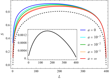
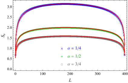
Figure 1: Left: leading term in the asymptotic approximation (30) to the von Neumann entanglement entropy of the sextic chain with $N=400$ spins for $a=0,10^{-3},10^{-2},10^{-1},\infty$ (the dashed black line represents the analogous quantity for the homogeneous XX chain). Inset: relative error between the $a=1$ and $a=\infty$ approximations. Right: Rényi entanglement entropy of the sextic chain with $N=400$ spins and $a=10^{-2}$ for $\alpha=1/4,1/2,3/4$, compared to its asymptotic approximation (30) (solid red lines).

Our numerical simulations indicate that the asymptotic formula (30)-(31) does indeed provide an excellent approximation to the Rényi entanglement of the sextic chain for $N\gg 1$ in the absence of a magnetic field and at half filling. For $\alpha<1$ this is illustrated by Fig. 1 (right), where we present the case of $N=400$ spins for $a=10^{-2}$ (for which the hopping amplitude is neither homogeneous nor approximately symmetric about the midpoint) and $\alpha=1/4,1/2,3/4$. Of course, in order to compare the asymptotic formula (30)-(31) with the exact (numerically computed) value of the entanglement entropy $S_{\alpha}$ it is necessary to first determine the constant part $c^{\prime}_{\alpha}$ in the former equation. We have simply estimated $c^{\prime}_{\alpha}$ as the average value of the difference between $S_{\alpha}$ and the leading term of its asymptotic approximation (30). Surprisingly, this value of $c^{\prime}_{\alpha}$ coincides to a remarkable accuracy with the corresponding one for the homogeneous XX chain given by Eq. (20) (see, e.g., Fig. 2 (left) for $a=10^{-2}$). In fact, we have checked that this is also the case for several other values of the parameter $a$.

As mentioned in the previous section, in the homogeneous XX chain the $o(1)$ term in the asymptotic formula (18) for the Rényi entanglement entropy with parameter $\alpha\geqslant\nobreak 1$ is oscillatory and of order $N^{{-1/\alpha}}$ (cf. Eqs. (23)-(24)). In particular, at half filling this term features parity oscillations with amplitude roughly proportional to $[(N/\pi)\sin(\pi L/N)]^{-1/\alpha}$. We have checked that the behavior of the Rényi entanglement entropy of the sextic chain with parameter $\alpha\geqslant 1$ at half-filling and zero magnetic field is very similar, and in particular that its parity oscillations are reproduced with great accuracy by Eqs. (30)-(31). This can be seen, for instance, in Fig. 2 (right), where we compare the Rényi entanglement entropy with parameter $\alpha=2$ for $a=10^{-2}$ and $N=400$ spins with its asymptotic approximation (30). Remarkably, in all the cases we have analyzed the values of the parameters $c_{\alpha}^{\prime}$ and $\mu_{\alpha}$ are very close to the corresponding ones for the homogeneous model, given by Eqs. (20) and (24). This suggests —as shall be further corroborated by the analysis of the Krawtchouk chain in the next section— that at half filling and in a vanishing (or constant) magnetic field the sextic chain is in the same universality class as the homogeneous XX chain.

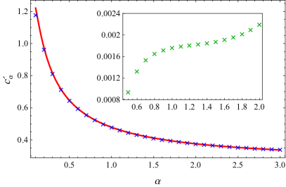
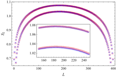
Figure 2: Left: constant term $c^{\prime}_{\alpha}$ in the asymptotic approximation (30)-(31) to the Rényi entanglement entropy $S_{\alpha}$ of the sextic chain with $a=10^{-2}$ and $N=400$ spins for $\alpha=i/10$ and $1\leqslant i\leqslant 30$ (blue crosses) compared to the corresponding constant $c^{\prime}_{\alpha}$ for the homogeneous XX chain in Eq. (20) (solid red line). The inset shows the difference between $c_{\alpha}^{\prime}$ and its counterpart (20) for the homogeneous chain in the range $1/2\leqslant\alpha\leqslant 2$ at intervals of $1/10$. Right: Rényi entanglement entropy $S_{2}$ for the sextic chain with $a=10^{-2}$ and $N=400$ spins at half filling and zero magnetic field (blue crosses) compared to its asymptotic approximation (30) (red squares). The inset shows a blow up of the range $150\leqslant L\leqslant 250$ in the latter plot.

The situation is markedly different in the presence of an inhomogeneous magnetic field and/or at arbitrary fillings. Indeed, our numerical calculations clearly indicate that in these cases the behavior of the Rényi entanglement entropy is not well described even to leading order by the conformal analogue of Eq. (21)-(22), namely

$$S_{\alpha}(N,\lambda)=\frac{1}{12}\,\big{(}1+\alpha^{-1}\big{)}\log f(N,\lambda)+c_{\alpha}^{\prime}+o(1)\,,$$ (42)

with

$$f(N,\lambda) =\frac{\widetilde{{\mathcal{L}}}}{\pi\Delta\widetilde{x}}\sin\left(\frac{\pi\widetilde{\ell}}{\widetilde{{\mathcal{L}}}}\right)\sin k_{F}$$

$$=\frac{2KN}{\pi\sqrt{a+1}}\,\sqrt{\lambda(1-\lambda)(a+\lambda)}\,\sin\left(\frac{\pi F\bigl{(}\arccos\sqrt{\lambda}\,\bigr{)}}{K}\right)\sin k_{F}\,.$$ (43)

Consider, to begin with, the case $\beta=0$ and $k_{F}\neq\pi/2$, illustrated in Fig. 3 (left) for the Fermi momentum $k_{F}=\pi/4$ and $a=10^{-2}$ or $a=1$. The fact that $k_{F}\neq\pi/2$ is seen to have two main effects. In the first place, $S_{\alpha}$ is now virtually zero for small $L$ and $N-L$ (for instance, if $N=400$ and $a=10^{-2}$ then $S_{2}$ is less than $10^{-3}$ for $1\leqslant L\leqslant 64$ and $393\leqslant L\leqslant 399$, while for $a=1$ we have $S_{2}<10^{-3}$ if $1\leqslant L\leqslant 31$ and $385\leqslant L\leqslant 399$). It is then clear that the entanglement entropy cannot be well approximated in this case by the concave function in the RHS of Eqs. (42)-(6). Moreover, for $\alpha\geqslant 1$ the parity oscillations of $S_{\alpha}$ are much less regular than in the case of half filling, and their amplitude is not well reproduced by a simple formula like (30) (see, e.g., the main plot in Fig. 3 (left) for the case $a=10^{-2}$, $\beta=0$, $k_{F}=\pi/4$, $N=400$ and $\alpha=2$). On the other hand, a rough approximation capturing only the average variation of $S_{\alpha}$ with $L$ can be obtained by restricting ourselves to the interval $[L_{1}+1,L_{2}-1]$ in which $S_{\alpha}$ differs significantly from zero, and replacing accordingly $L$ and $N$ respectively by $L-L_{1}$ and $L_{2}-L_{1}$. With these changes Eq. (6) becomes

$$f(N,\lambda)=\frac{2K(L_{2}-L_{1})}{\pi\sqrt{a+1}}\,\sqrt{\lambda_{\text{eff}}(1-\lambda_{\text{eff}})(a+\lambda_{\text{eff}})}\,\sin\left(\frac{\pi F\bigl{(}\arccos\sqrt{\lambda_{\text{eff}}}\,\bigr{)}}{K}\right)\sin k_{F}\,,$$ (44)

with

$$\lambda_{\text{eff}}=\frac{L-L_{1}}{L_{2}-L_{1}}=\frac{N\lambda-L_{1}}{L_{2}-L_{1}}\,.$$ (45)

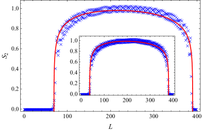
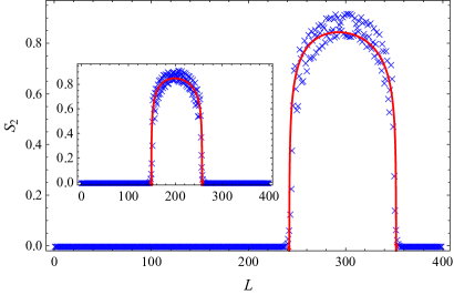
Figure 3: Left: Rényi entanglement entropy $S_{2}$ for the sextic chain with $N=400$ spins, $a=10^{-2}$, $\beta=0$, and $k_{F}=\pi/4$ (blue crosses) compared to its rough approximation (42)-(44) (solid red line). The inset shows the same plot for $a=1$. Right: Analogous plot for $a=10^{-2}$, $\beta=5$ and $k_{F}=\pi/4$ (main plot) or $k_{F}=\pi/2$ (inset).

The rough approximation (42)-(44) is represented by a red line in Fig. 3.

The situation is qualitatively similar in the presence of an external magnetic field given by Eq. (35) with $\beta\neq 0$, even in the case of half filling; see, e.g., Fig. 3 (right). More precisely, as seen in the latter figure, the length of the intervals in which $S_{\alpha}$ is practically zero increases significantly with $\beta$. Moreover, when $k_{F}$ differs from $\pi/2$ the interval over which $S_{\alpha}$ is appreciably different from zero is translated by an amount depending on $\beta$. As before, the pattern of the parity oscillations is much more involved than in the case $B_{n}=0$, $k_{F}=\pi/2$ analyzed earlier, although the average variation of $S_{\alpha}$ with $L$ is still reproduced to a certain extent by the heuristic formula (42)-(44).

Note, finally, that the fact that the entropy of the block $\{0,\dots,L-1\}$ is negligibly small for $L\leqslant L_{1}$ and $L\geqslant L_{2}$ clearly indicates that the first $L_{1}$ and last $N-L_{2}$ spins are approximately in a product state, so that the chain’s entanglement is almost entirely concentrated in the central block $\{L_{1},\dots,L_{2}-1\}$. It would certainly be of interest to understand how exactly this phenomenon arises as the external magnetic field is turned on, or the standard filling $M/N=1/2$ is varied.

7 The Krawtchouk chain

7.1 Definition and entanglement entropy

The Krawtchouk chain was introduced in Ref. CNV19 in connection with the family of discrete Krawtchouk polynomials. More precisely, the Krawtchouk polynomial $K_{n}(x;q,m)$ is defined as

$$K_{n}(x;q,m)={}_{2}F_{1}(-n,-x;-m;1/q)\,,\qquad n=0,\dots,m\,,$$ (46)

where $0<q<1$ and $m$ is a nonnegative integer (see, e.g., KLS10 ). Here ${}_{2}F_{1}$ denotes the standard hypergeometric function

$${}_{2}F_{1}(a,b;c;z):=\sum_{k=0}^{\infty}\frac{(a)_{k}(b)_{k}}{(c)_{k}}\,\frac{z^{k}}{k!}\,,$$

where $(a)_{k}:=a(a+1)\cdots(a+k-1)$ is the usual (ascending) Pochhammer symbol. These polynomials satisfy the recursion relation

$$A_{n}K_{n+1}(x)=(B_{n}-x)K_{n}(x)-C_{n}K_{n-1}(x)$$

with

$$A_{n}=q(m-n)\,,\qquad B_{n}=n(1-q)+q(m-n)\,,\qquad C_{n}=n(1-q)\,.$$

The corresponding monic polynomials are given by

$$P_{n}(x)=\prod_{k=0}^{n-1}(-A_{k})\cdot K_{n}(x;q,m)=(-q)^{n}(m-n+1)_{n}K_{n}(x;q,m)\,,$$

and satisfy the normalized recursion relation

$$P_{n+1}(x)=(x-B_{n})P_{n}(x)-a_{n}P_{n-1}(x)$$

with $B_{n}$ as before and

$$a_{n}=A_{n-1}C_{n}=q(1-q)n(m-n+1)>0\,,\qquad 1\leqslant n\leqslant m\,.$$

The polynomial $K_{m+1}(x;q,m)$ cannot be defined through Eq. (46), since $(-m)_{m+1}=0$. On the other hand, we can use the previous recursion relation with $n=m$ to define $P_{m+1}$ by

$$P_{m+1}(x)=\big{[}x-m(1-q)\big{]}P_{m}(x)-mq(1-q)P_{m-1}(x)\,.$$

Using the previous formula and the recursion relation, after a long but straightforward calculation we obtain

$$P_{m+1}(x)=\prod_{k=0}^{m}(x-k)\,.$$

In view of the above, we define the Krawtchouk chain through the polynomials $P_{n}(x)$ with $m=N-1$. In other words, the chain’s parameters $J_{n}$ and $B_{n}$ are given by

$$J_{n} =\sqrt{a_{n+1}}=\sqrt{q(1-q)(n+1)(N-n-1)}\,,$$ (47)

$$B_{n} =n(1-q)+q(N-n-1)=q(N-1)+(1-2q)n\,.$$ (48)

In particular, the magnetic field is constant if and only if $q=1/2$. Using the definition of the Krawtchouk polynomials we readily obtain the explicit formula

$$P_{n}(E)=(N-n)_{n}\sum_{k=0}^{n}\frac{\binom{n}{k}}{\binom{N-1}{k}}\,\frac{(-q)^{n-k}}{k!}\,E(E-1)\cdots(E-k+1)\,,\qquad n=0,\dots,N-1\,,$$

with $P_{N}(E)=E(E-1)\cdots(E-N+1)$. Thus in this case the single-particle energies $\varepsilon_{k}$ are simply the integers $0,1,\dots,N-1$. This makes it possible to express the matrix elements $\Phi_{nk}$ in closed form using Eqs. (15)-(16). Indeed, it is readily found that

$$\gamma_{n}=q^{n}(1-q)^{n}n!(N-n)_{n}\,,\qquad w_{k}=\binom{N-1}{k}q^{k}(1-q)^{N-1-k}\,,$$

and therefore

$$\Phi_{nk} =\frac{1}{n!}\sqrt{\frac{\binom{N-1}{k}}{\binom{N-1}{n}}}\,q^{\frac{1}{2}(k-n)}(1-q)^{\frac{1}{2}(N-k-n-1)}\,P_{n}(k)$$

$$=(-1)^{n}\sqrt{\binom{N-1}{k}\binom{N-1}{n}}\,q^{\frac{1}{2}(k+n)}(1-q)^{\frac{1}{2}(N-k-n-1)}\,K_{n}(k;q,N-1)\,.$$ (49)

Dropping the irrelevant overall factor $[q(1-q)]^{1/2}(N-1)$ in Eq. (47) we easily obtain the following formula for the continuum limit of $J_{n}$:

$$J(x)=\sqrt{p(x/{\mathcal{L}})}\,,\qquad p(\xi):=\sqrt{\xi(1-\xi)}\,.$$

We thus have

$$\widetilde{x}(x)={\mathcal{L}}\int_{0}^{x/{\mathcal{L}}}\frac{d\xi}{\sqrt{\xi(1-\xi)}}=2{\mathcal{L}}\arcsin\bigl{(}{\textstyle\sqrt{x/{\mathcal{L}}}}\,\bigr{)}\,,\qquad\widetilde{{\mathcal{L}}}=\pi{\mathcal{L}}\,,$$ (50)

and hence the function $f(N,\lambda)$ in Eq. (31) is simply given by

$$f(N,\lambda)=N\sqrt{\lambda(1-\lambda)}\,\sin(2\arcsin\sqrt{\lambda})=2N\lambda(1-\lambda)\,.$$ (51)

As expected, this result coincides with the $a\to\infty$ limit of the analogous function for the sextic chain. In other words, the asymptotic behavior of the entanglement entropy of the Krawtchouk chain with $q=1/2$ at half filling, given by Eqs. (30)-(51), should be the same as for the sextic chain with $\beta=0$ and $a\gg 1$. This is shown in Fig. 4 (left) for $N=400$ spins. For the same reason, at arbitrary fillings the heuristic asymptotic approximation to the entanglement entropy is given by Eq. (42) with

$$f(N,\lambda)=\frac{2(N\lambda-L_{1})(L_{2}-N\lambda)}{L_{2}-L_{1}}\,\sin k_{F}\,,$$ (52)

where $[L_{1}+1,L_{2}-1]$ is the interval over which $S_{\alpha}$ is appreciably nonzero; see, e.g., the inset of Fig. 4 (left). Note also that when $q=1/2$ we have $J_{n}=J_{N-n-2}$ and $B_{n}$ is constant, so that in this case the entanglement entropy is invariant under $L\mapsto N-L$, i.e., satisfies Eq. (41), for all fillings.

On the other hand, for $q\neq 1/2$ the magnetic field strength $B_{n}$ is non-uniform, so that the entanglement entropy behaves much the same as for the sextic chain with $a\gg 1$ and $\beta\neq 0$; see, e.g., Fig. 4 (right) for the case $q=1/4$ and $N=400$. The main difference, as seen in the right inset of the latter figure, is that in this case the entropy is close to zero only on an interval of the form $[L_{2},N]$.

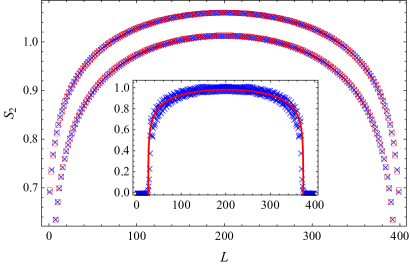
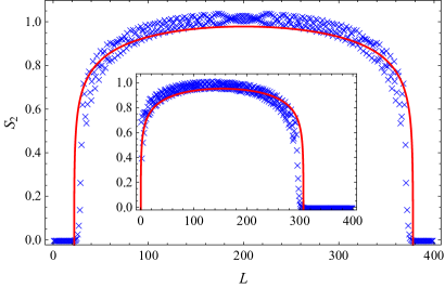
Figure 4: Left: Rényi entanglement entropy $S_{2}$ for the Krawtchouk chain with $q=1/2$ and $N=400$ spins at half filling (blue crosses) compared to its asymptotic approximation (30)-(51) (red squares). The inset shows a similar plot for $k_{F}=\pi/4$, compared to its heuristic approximation (42)-(52). Right: analogous plot for $q=1/4$ at half filling (main plot) and for $k_{F}=\pi/4$ (inset).

Remark 2.

The value of the subleading (constant) term $c_{\alpha}^{\prime}$ in the asymptotic formula (30)-(51) for the entanglement entropy of the Krawtchouk chain with $q=1/2$ at half filling is remarkably close to its counterpart $c_{\alpha,\text{hom}}^{\prime}$ for the homogeneous chain (cf. Eq. (20)), even more so than in the case of the sextic chain discussed above. For instance, the difference $|c_{\alpha}^{\prime}-c_{\alpha,\text{hom}}^{\prime}|$ is of the order of $10^{-3}$ or less for $1/2\leqslant\alpha\leqslant 2$. In fact, the values of $c_{\alpha}^{\prime}$ in the latter range were obtained as in the previous example by taking the average of the differences $S_{\alpha}-S_{\alpha,\text{app}}$ for all values of the block size $L=1,\dots,N-1$, where $S_{\alpha,\text{app}}$ denotes the leading term in Eq. (30). The behavior of the latter differences, however, clearly suggests that in this case a more accurate estimate for $c_{\alpha}^{\prime}$ is given by the average of $S_{\alpha}-S_{\alpha,\text{app}}$ for the central block sizes $L=N/2$ and $L=N/2-1$, or more simply by

$$c_{\alpha^{\prime}}=\frac{1}{2}\left(S_{\alpha}\Big{|}_{L=N/2-1}+S_{\alpha}\Big{|}_{L=N/2}\right)-S_{\alpha,\text{app}}\Big{|}_{L=N/2}\,;$$ (53)

see, e.g., Fig. 5 (left) for $\alpha=1$. The previous equation actually yields a value of $c_{\alpha}^{\prime}$ much closer to $c_{\alpha,\text{hom}}^{\prime}$ than the average of the differences $S_{\alpha}-S_{\alpha,\text{app}}$ for all block sizes. For instance, for $\alpha=1$ the difference between $c_{1,\text{hom}}^{\prime}$ and the value of $c_{1}^{\prime}$ computed from the previous formula is $1.1\cdot 10^{-6}$, compared to $3.6\cdot 10^{-4}$ when $c_{1}^{\prime}$ is estimated by the average of $S-S_{\text{app}}$ over all block sizes.

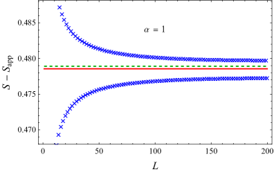
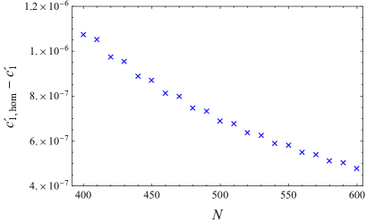
Figure 5: Left: difference between the von Neumann entanglement entropy $S$ of the Krawtchouk chain with $q=1/2$, $N=400$, $k_{F}=\pi/2$ and its leading asymptotic approximation $S_{\text{app}}:=(1/6)\log f(N,\lambda)$ as a function of the block size $L$. (Only the range $L=1,\dots,N/2$ has been represented, since in this case $S_{\alpha}$ is symmetric under $L\mapsto N-L$.) The height of the red (resp. green dashed) horizontal line is the value of $c_{1}^{\prime}$ computed from Eq. (53) (resp. as the average of the differences $S-S_{\text{app}}$ for all block sizes). Right: Difference $c_{1,\text{hom}}^{\prime}-c_{1}^{\prime}$ for $N=400,\dots,600$ in increments of 10.

We have also studied how the difference $c_{\alpha,\text{hom}}-c_{\alpha}^{\prime}$ varies as the number of spins increases from $N=400$ to $N=600$ (in increments of $10$) for several values of $\alpha$, where in view of the previous remark we have used Eq. (53) to estimate $c_{\alpha}^{\prime}$. As is apparent from Fig. 5 (right) for the case $\alpha=1$, the absolute value of this difference steadily decreases with $N$. We thus conjecture that for the Krawtchouk chain with $q=1/2$ at half filling the constant term $c_{\alpha}^{\prime}$ tends to $c_{\alpha,\text{hom}}^{\prime}$ as the number of spins tends to infinity. A similar analysis for the sextic chain (with $a=10^{-2}$) also shows a decrease in $|c_{\alpha,\text{hom}}-c_{\alpha}^{\prime}|$ as $N$ increases in the same range, although the value of this difference is about three orders of magnitude higher than in the case of the Krawtchouk chain. This different behavior could be explained by the fact that the sextic chain is not invariant under $J_{n}\mapsto J_{N-n-2}$, as are the homogeneous and Krawtchouk chains. In fact, the latter two chains are the only XX spin chains of algebraic type (in the more general sense that the recursion coefficients $a_{n}$ are polynomial in $n$) with interactions $J_{n}$ invariant under $n\mapsto N-n-2$ having a finite total conformal length $\tilde{\mathcal{L}}$.

Remark 3.

The plots in Fig. 4 suggest that the entanglement entropy of the Krawtchouk chain is invariant under $L\mapsto N-L$ not only for $q=1/2$ (at arbitrary filling), but also for arbitrary $q$ at half filling. That this is indeed the case can be deduced from a general property of the entanglement entropy, stemming from the fact that $\widehat{J}_{n}:=J_{N-n-2}=J_{n}$ and $B_{n}$ is linear in $n$. Indeed, setting $B_{n}=B_{0}+bn$, with $B_{0}$ and $b$ independent of $n$, we have

$$\widehat{B}_{n}:=B_{N-n-1}=2B_{0}+b(N-1)-B_{n}.$$

From the previous equations for $\widehat{J}_{n}$ and $\widehat{B}_{n}$ we immediately obtain the following relation for the corresponding polynomials $\widehat{P}_{n}$:

$$\widehat{P}_{n}(x)=(-1)^{n}P_{n}\Bigl{(}2B_{0}+b(N-1)-x\Bigr{)}.$$

This is readily seen to imply that

$$\widehat{\Phi}_{nk}=(-1)^{n}\Phi_{n,N-k-1}\,,$$

which yields the relation

$$\widehat{C}_{mn}[\{0,\dots,L-1\};\{0,\dots,M-1\}]=C_{mn}[\{N-L,\dots,N-1\};\{0,\dots,M-1\}]\\ =(-1)^{m+n}C_{mn}[\{0,\dots,L-1\};\{N-M,\dots,N-1\}],$$

where the first argument denotes the block of spins considered and the second one the energy modes excited. Since the matrices $(A_{mn})$ and $((-1)^{m+n}A_{mn})$ are obviously similar, we deduce that

$$S_{\alpha}[\{0,\dots,N-L-1\};\{0,\dots,M-1\}] =S_{\alpha}[\{N-L,\dots,N-1\};\{0,\dots,M-1\}]$$

$$=S_{\alpha}[\{0,\dots,L-1\};\{N-M,\dots,N-1\}]\,,$$

where in the first equality we have applied the well-known invariance of the entanglement entropy under complements in position space. On the other hand, from the energy-position duality of the entanglement entropy LYQ14 ; HA12 ; CFGT17 it follows that $S_{\alpha}$ is also invariant under complements in energy space. We thus obtain the relation

$$S_{\alpha}[\{0,\dots,N-L-1\};\{0,\dots,M-1\}]=S_{\alpha}[\{0,\dots,L-1\};\{0,\dots,N-M-1\}].$$ (54)

In particular, this implies that at half filling $S_{\alpha}$ is invariant under $L\mapsto N-L$, as claimed. Of course, for the Krawtchouk chain with $q=1/2$ we can combine Eqs. (41) and (54) to deduce that $S_{\alpha}$ is also invariant under $M\mapsto N-M$ (this also follows from a standard duality argument). Note, finally, that since the couplings of the sextic chain with $a\gg 1$ are approximately symmetric under $n\mapsto N-n-2$, and its magnetic field term $B_{n}$ is linear in $n$, Eq. (54) is approximately valid also in this case.

7.2 Ground state energy

In Ref. MSR21 it is conjectured that as $N\to\infty$ the ground state energy $E_{0}(N)$ of an inhomogeneous XX chain (1) with $B_{n}=0$ for all $n$ behaves as

$$E_{0}(N)=-c_{0}\Sigma_{N}-c_{B}(J_{0}+J_{N-2})-\frac{\pi v_{F}}{24\widetilde{\mathcal{N}}}+O(N^{-2})\,,$$ (55)

where $\widetilde{\mathcal{N}}=\widetilde{{\mathcal{L}}}/\Delta x$,

$$\Sigma_{N}:=\sum_{n=0}^{N-2}J_{n}\,,$$

and $c_{0}$, $c_{B}$, $v_{F}$ are three constants (representing the bulk energy per site, the boundary energy and the Fermi velocity) which in the homogeneous case take the respective values $2/\pi$, $4/\pi-1$, and $2$ Ca84 ; BCN86 . In the absence of a magnetic field the ground state is the half-filled state (11), whose energy $E_{0}(N)$ is given by Eq. (12). This quantity can be exactly computed for the Krawtchouk chain with $q=1/2$, since its single-particle energies (after subtraction of the constant magnetic field $B_{n}=(N-1)/2$) are given by the formula

$$\varepsilon_{k}=k-\frac{1}{2}\,(N-1)\,,\qquad 0\leqslant k\leqslant N-1\,,$$

whence

$$E_{0}(N)=-\frac{N^{2}}{8}\,.$$ (56)

We shall next compare this exact value for $E_{0}(N)$ with its conjectured asymptotic expansion (55), which by Eqs. (47) and (50) reads in this case

$$E_{0}(N)=-c_{0}\Sigma_{N}-c_{B}\sqrt{N-1}-\frac{v_{F}}{24N}+O(N^{-2})\,.$$ (57)

Using the exact value (56) for $E_{0}(N)$ we deduce that in this case

$$c_{0}\Sigma_{N}=\frac{N^{2}}{8}-c_{B}\sqrt{N-1}-\frac{v_{F}}{24N}+O(N^{-2})\,.$$ (58)

On the other hand, the leading asymptotic behavior as $N\to\infty$ of the sum

$$\Sigma_{N}=\frac{1}{2}\sum_{n=0}^{N-2}\sqrt{(n+1)(N-n-1)}=\frac{1}{2}\sum_{n=1}^{N-1}\sqrt{n(N-n)}$$

can be determined from the Euler–Maclaurin formula Kn51

$$2\Sigma_{n}-\int_{1}^{N-1}g(x)\,\mathrm{d}x =\frac{1}{2}\,[g(N-1)+g(1)]+\frac{1}{2}\,[g^{\prime}(N-1)-g^{\prime}(1)]+R_{3}$$

$$=g(1)-g^{\prime}(1)+R_{3}=\sqrt{N-1}-\frac{N/2-1}{\sqrt{N-1}}+R_{3}\,,$$

where $g(x):=\sqrt{x(N-x)}$. The remainder $R_{3}$ can be estimated as

$$|R_{3}| \leqslant\frac{\zeta(3)}{4\pi^{3}}\int_{1}^{N-1}|g^{\prime\prime\prime}(x)|\mathrm{d}x=\frac{\zeta(3)}{2\pi^{3}}\int_{1}^{N/2}g^{\prime\prime\prime}(x)\mathrm{d}x=\frac{\zeta(3)}{2\pi^{3}}\,[g^{\prime\prime}(N/2)-g^{\prime\prime}(1)]$$

$$=\frac{\zeta(3)}{8\pi^{3}}\,N^{2}\big{[}(N-1)^{-3/2}-8N^{-3}\big{]}=O(N^{1/2})\,,$$

where $\zeta(s)$ denotes Riemann’s zeta function. We also have

$$\int_{0}^{N}g(x)\,\mathrm{d}x=N^{2}\int_{0}^{1}\sqrt{t(1-t)}\,\mathrm{d}t=\frac{\pi N^{2}}{8}\,,$$

and hence

$$\int_{1}^{N-1}g(x)\,\mathrm{d}x=\frac{\pi N^{2}}{8}-2\int_{0}^{1}\sqrt{x(N-x)}\,\mathrm{d}x=\frac{\pi N^{2}}{8}+O(N^{1/2})\,.$$

We thus conclude that

$$\Sigma_{N}=\frac{\pi N^{2}}{16}+O(N^{1/2})\,,$$

in agreement with the right-hand side of Eq. (58) if we take $c_{0}=2/\pi$ (as in the homogeneous case).

It can be shown that the higher-order corrections in the Euler–Maclaurin formula are all $O(N^{1/2})$, so that they cannot be used to compute $c_{B}$ and $v_{F}$ in closed form (this is essentially due to the fact that the derivatives of $g(x)$ diverge at $x=0,N$). On the other hand, the parameter $c_{B}$ can be computed through the formula

$$c_{B}=\lim_{N\to\infty}\frac{1}{\sqrt{N-1}}\,\bigg{(}\frac{N^{2}}{8}-\frac{2\Sigma_{N}}{\pi}\bigg{)}\,.$$

By evaluating the right-hand side for large values of $N$ we have verified that this limit indeed exists, and that $c_{B}=0.1323449$ to seven decimal places. Note that this value is about one half of the corresponding one for the homogeneous case.

Using the previous estimate for the constant $c_{B}$, we have studied the behavior of the difference $N^{2}/8-2\Sigma_{N}/\pi-c_{B}\sqrt{N-1}$

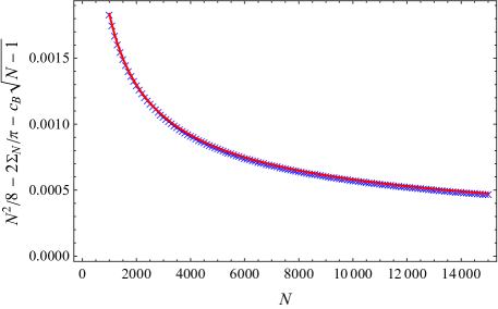
Figure 6: Difference $N^{2}/8-2\Sigma_{N}/\pi-c_{B}\sqrt{N-1}$ with $c_{B}=0.1323449$ for $N$ in the range $[1000,15000]$ in increments of 100 (blue crosses), compared to the curve $0.0580365/\sqrt{N}$ (red line).

for $1000\leqslant N\leqslant 15000$, obtaining very strong numerical evidence that it is of order $N^{-1/2}$ instead of $N^{-1}$, as predicted by Eq. (58) (cf. Fig. 6). In other words, our results suggest that for the Krawtchouk chain (with $q=1/2$) Eq. (57) should be replaced by

$$E_{0}(N)=-c_{0}\Sigma_{N}-c_{B}\sqrt{N-1}-\frac{k}{\sqrt{N}}+o(N^{-1/2})\,,$$

with $k\simeq 0.0580365$.

8 The Lamé chain

We shall next study the chain associated to the quantum (finite gap) Lamé potential introduced in Ref. FG20 , whose parameters are given by

$$J_{n}=\sqrt{(n+1)(N-n-1)(n+1/2)(N-n-3/2)}\,,\qquad B_{n}=0\,.$$ (59)

Although an approximation to the entanglement entropy of this chain at half filling was obtained in Ref. FG20 , for the sake of consistency we shall next outline the derivation of an equivalent formula using the present approach and notation. To this end, we first write

$$J_{n}=(N-1)^{2}\sqrt{\bigg{(}\frac{x_{n}}{{\mathcal{L}}}+\varepsilon\bigg{)}\bigg{(}1-\frac{x_{n}}{{\mathcal{L}}}\bigg{)}\bigg{(}\frac{x_{n}}{{\mathcal{L}}}+\frac{\varepsilon}{2}\bigg{)}\bigg{(}1-\frac{x_{n}}{{\mathcal{L}}}-\frac{\varepsilon}{2}\bigg{)}}\,,\qquad\varepsilon:=\frac{1}{N-1}\,,$$

and thus (up to an irrelevant constant factor)

$$J(x)=\sqrt{p(x/{\mathcal{L}})}\,,\qquad p(\xi):=(\xi+\varepsilon)(\xi+\varepsilon/2)(1-\xi-\varepsilon/2)(1-\xi)\,.$$ (60)

Note that in this case we cannot just take $\varepsilon=0$, since the integral of $1/J(x)$ would then diverge at $x=0,{\mathcal{L}}$. It is also worth mentioning that in this case we cannot extend the range of $\xi$ all the way to $1$, since $p(\xi)$ is negative for $\xi>1-\varepsilon/2$. To evaluate the integral (33) we perform the change of variable $\xi=(z+1-\varepsilon)/2$, obtaining

$$\int_{0}^{s}\frac{\mathrm{d}\xi}{\sqrt{(\xi+\varepsilon)(\xi+\frac{\varepsilon}{2})(1-\xi-\frac{\varepsilon}{2})(1-\xi)}} =2k\int_{-1+\varepsilon}^{2s-1+\varepsilon}\frac{\mathrm{d}z}{\sqrt{(1-z^{2})(1-k^{2}z^{2})}}$$

$$=2k\Big{[}F\Bigl{(}\arcsin(2s-1+\varepsilon)\Bigr{)}+F\Bigl{(}\arcsin(1-\varepsilon)\Bigr{)}\Big{]},$$

where the modulus of the elliptic integral is

$$k:=(1+\varepsilon)^{-1}=1-\frac{1}{N}<1\,.$$

We thus have

$$\widetilde{x}(x)=2k{\mathcal{L}}\Big{[}F\Bigl{(}\arcsin(2\xi-1+\varepsilon)\Bigr{)}+F\Bigl{(}\arcsin(1-\varepsilon)\Bigr{)}\Big{]},\qquad\xi:=x/{\mathcal{L}}\,.$$

In order to compute the chain’s conformal length $\widetilde{{\mathcal{L}}}$ we must specify the upper limit of the variable $\xi$, which in this case cannot be extended to $1$ for the reason explained above. In fact, although the integrand in Eq. (33) remains real up to $\xi=1-\varepsilon/2$, it is more convenient (and of no consequence in the limit $N\to\infty$) to use the symmetric interval $-1+\varepsilon\leqslant\xi\leqslant 1-\varepsilon$. With this choice we obtain

$$\widetilde{{\mathcal{L}}}=4k{\mathcal{L}}F\Bigl{(}\arcsin(1-\varepsilon)\Bigr{)},$$

from which it follows that

$$\sin\left(\frac{\pi\widetilde{\ell}}{\widetilde{{\mathcal{L}}}}\right)=\cos\left(\frac{\pi F\left(\arcsin(2\lambda-1+\varepsilon)\right)}{2F\left(\arcsin(1-\varepsilon)\right)}\right).$$

For $0<\lambda<1$ the numerator of the argument of the cosine tends to the finite limit $F(\arcsin(2\lambda-1),1)=\operatorname{arctanh}(2\lambda-1)$ as $N\to\infty$ (i.e., $\varepsilon\to 0+$), while the denominator tends to $K(1)=+\infty$. Thus for sufficiently large $N$ we can take the function $f$ in Eq. (31) simply as

$$f(N,\lambda)\simeq\frac{N\widetilde{{\mathcal{L}}}/{\mathcal{L}}}{\pi}\,J(\ell)\simeq\frac{4N}{\pi}\,F\Bigl{(}\arcsin(1-\varepsilon)\Bigr{)}\lambda(1-\lambda),$$ (61)

up to lower-order terms in $N$. Note that $f(N,\lambda)$ is invariant under $\lambda\mapsto 1-\lambda$, which is consistent with the symmetry of the coupling (59) with respect to the chain’s midpoint. It can be shown that in the $N\to\infty$ limit we have

$$F\Bigl{(}\arcsin(1-\varepsilon)\Bigr{)}=\frac{1}{2}\log(2N)+\kappa+o(1)\,,$$

with $\kappa=0.1882264\dots$, so that $f(N,\lambda)\sim N\log N$ in this limit. Thus when $N\to\infty$ with $\lambda$ fixed the entanglement entropy of the Lamé chain (59) at half filling should behave as

$$S_{\alpha}(N,\lambda)=\frac{1}{2}\,(1+\alpha^{-1})\log[N\lambda(1-\lambda)]+O\bigl{(}\log(\log N)\bigr{)}.$$ (62)

Equation. (61) is in agreement up to lower order terms with the analogous equation in Ref. FG20 , obtained by replacing $F(\arcsin(1-\varepsilon))$ by $K$, since OLBC10

$$K\Bigl{(}(1+\varepsilon)^{-1}\Bigr{)}=\frac{1}{2}\log(8N)+o(1).$$

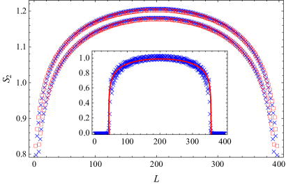
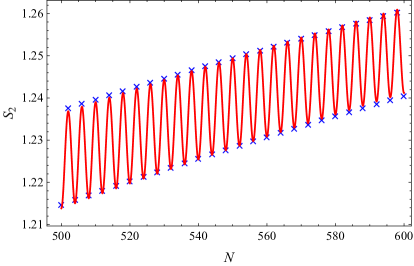
Figure 7: Left: Rényi entanglement entropy with parameter $\alpha=2$ for the Lamé chain with $N=400$ spins at half filling (blue crosses) compared to its asymptotic approximation (30)-(61) (red squares). The inset shows the analogous plot for the Fermi momentum $k_{F}=\pi/4$ compared to the heuristic approximation (42)-(63) (red line). Right: Rényi entanglement entropy $S_{2}$ for the Lamé chain with $\lambda=1/2$ for an even number of spins $N$ in the interval $[500,600]$ at half filling (blue crosses) compared to its approximation (30)-(61) with $(-1)^{L}$ replaced by $\sin((2L+1)\pi/2)$ (red line).

It should also be noted that the logarithmic divergence of $f(N,\lambda)/N$ as $N\to\infty$ with $\lambda$ fixed is due to the presence of double zeros of $J(x)$ at both endpoints of the interval $[0,{\mathcal{L}}]$ in this limit, and can thus only happen when the polynomial $p(\xi)$ in Eq. (32) is of degree four.

We have numerically checked that the asymptotic formula (30)-(61) still provides a reasonable approximation to the entanglement entropy at half filling in this case, though not as precise as for the sextic and Krawtchouk chains. In particular, the oscillating term proportional to $f(N,\lambda)^{-1/\alpha}$ in Eq. (30) reproduces with acceptable accuracy the parity oscillations in $S_{\alpha}$ present when $\alpha\geqslant 1$ (see, e.g., Fig. 7 (left) for $\alpha=2$ and $N=400$ spins). As before, at Fermi momenta $k_{F}\neq\pi/2$ the Rényi entanglement entropy $S_{\alpha}$ is virtually zero over two intervals of the form $[1,L_{1}]$ and $[N-L_{1},N-1]$, and the asymptotic formula (30)-(61) fails. However, proceeding as above we can derive a rough heuristic approximation to $S_{\alpha}$ in the interval $[L_{1}+1,N-L_{1}-1]$ using Eq. (42) with

$$f(N,\lambda)=\frac{4(N-2L_{1})}{\pi}\,F\Bigl{(}\arcsin(1-\varepsilon_{\text{eff}}),(1+\varepsilon_{\text{eff}})^{-1}\Bigr{)}\lambda_{\text{eff}}(1-\lambda_{\text{eff}})\sin k_{F}\,,$$ (63)

with $\lambda_{\text{eff}}$ given by Eq. (45) with $L_{2}=N-L_{1}$ and $\varepsilon_{\text{eff}}=(N-2L_{1}-1)^{-1}$.

Since the dependence on the number spins $N$ of the asymptotic formula (30)-(61) for the entanglement entropy at half filling is nontrivial, it is also of interest to study the growth of $S_{\alpha}(N,\lambda)$ with $N$ for fixed values of $\lambda$. We have checked that the latter formula captures the behavior of $S_{\alpha}(N,\lambda)$ with great accuracy, and in particular reproduces the parity oscillations that appear when $\alpha\geqslant 1$ (see, e.g., Fig. 7 (right) for the case $\lambda=1/2$ and even $N$ in the interval $[500,600]$). Remarkably, although the two parameters $c_{\alpha}^{\prime}$ and $\mu_{\alpha}$ appearing in Eq. (30) are fitted, they turn out to be of the same order of magnitude as their counterparts (20)-(24) for the homogeneous XX chain. Note, however, that in this case it should not be expected that the constant term $c_{\alpha}^{\prime}$ tend to $c_{\alpha,\text{hom}}^{\prime}$ as $N\to\infty$, since the subleading term in the asymptotic expansion of $S_{\alpha}$ is no longer constant but of the order of $\log(\log N)$ (cf. Eq. (62)).

9 Conclusions and outlook

In this work we study a large class of inhomogeneous XX spin chains whose squared couplings are a polynomial of degree at most four in the site index. This class includes some previously studied models related to classical Krawtchouk and dual Hahn polynomials CNV19 , as well as the inhomogeneous XX chains related to QES models on the line classified in Ref. FG20 . We show how to exactly compute the leading term in the asymptotic expansion of the block entanglement entropy of these models (in a constant magnetic field at half filling) from their continuum limit, which coincides with the CFT of a massless Dirac fermion in a curved ($1+1$)-dimensional background DSVC17 ; RDRCS17 ; TRS18 . We next focus on three inhomogeneous chains with algebraic interactions, associated to the sextic oscillator QES potential, the Krawtchouk polynomials and the periodic quantum Lamé potential. We exploit the relation of XX chains with finite families of orthogonal polynomials to numerically compute the Rényi entanglement entropy of the latter chains for a large number of spins. When the Rényi parameter $\alpha$ is less than one we find that, as expected, the asymptotic formula reproduces with great accuracy the behavior of the entanglement entropy. On the other hand, for $\alpha\geqslant 1$ the Rényi entropy presents parity oscillations whose amplitude increases with $\alpha$, as is known to be the case for the homogeneous XX chain FC11 . We show that these oscillations are reproduced with excellent accuracy by the Fagotti–Calabrese formula for the homogeneous chain FC11 , replacing the block’s and the chain’s length by their conformal counterparts. In fact, for the sextic and Krawtchouk chains (at half filling and in a constant magnetic field) we have found rather compelling numerical evidence that the subleading non-universal (constant) term in the asymptotic expansion of the entanglement entropy tends to its counterpart for the homogeneous XX chain as the number of spins tends to infinity. We conjecture that this is actually the case for the class of algebraic chains studied in this paper when the chain’s conformal length is finite, i.e., when the squared couplings considered as functions of the site index $n$ have no multiple real roots in the interval $[0,N]$.

All of the above results apply to the case of half filling and constant magnetic field, which is the one usually considered in the literature in the inhomogeneous case. In this work we have also studied in some detail the non-standard situation of arbitrary filling and/or inhomogeneous magnetic field. We have found that the main difference with the standard situation is that the block entanglement entropy vanishes when the block’s length is either small or close to the chain’s length. Thus at fillings other than one-half, or in an inhomogeneous magnetic field, the first few and last spins in the chain become disentangled from the rest. This is in fact one of the paper’s main results, which certainly deserves further theoretical analysis. Another interesting feature of the non-standard case is that the oscillations of the entropy when $\alpha\geqslant 1$ are considerably more complex than in the standard one, and in particular are not well described by a modification of the Fagotti–Calabrese formula along the lines mentioned above.

One of the models studied in this paper, namely the Krawtchouk chain (cf. Section 7), has the rather unusual property that its single-particle energies at zero magnetic field can be exactly computed (they are simply the numbers $-(N-1)/2+k$, with $0\leqslant k\leqslant N-1$). This of course makes it trivial to evaluate the ground-state energy in closed form for an arbitrary number of spins $N$. We have compared this exact result with the recently proposed asymptotic expansion in Ref. MSR21 , finding that they match only to leading order.

The above results clearly suggest several avenues for future research that we shall now briefly outline. To begin with, we would like to find a theoretical justification of the fact that the constant term in the asymptotic expansion of the entanglement entropy of chains with algebraic interactions and finite conformal length (at half filling and in a constant magnetic field) seems to coincide with the analogous term for the homogeneous XX model in the limit of large $N$. An outstanding open problem of considerable interest is that of deriving an asymptotic formula for the leading behavior of the entanglement entropy in the non-standard scenario of arbitrary filling and/or inhomogeneous magnetic field. Our numerical results show that any such formula must necessarily vanish when the block length is either small or close to the chain’s length. Likewise, it would also be of interest to find a formula describing the entropy’s complex oscillations when the Rényi parameter is greater than or equal to one, akin to the Fagotti–Calabrese formula for the homogeneous chain. As mentioned in the Introduction, in the homogeneous case the behavior of the multiblock entanglement entropy has been thoroughly analyzed (see, e.g., CH09 ; CCT09 ; ATC10 ; AEF14 ; CFGT17 ). Again, the generalization of some of these results to the inhomogeneous case would certainly be worth exploring. Finally, another problem suggested by the present work is to understand why the asymptotic formula in Ref. MSR21 for the ground-state energy of inhomogeneous XX spin chains at zero magnetic field fails to reproduce the subleading behavior of the Krawtchouk chain, and how it should be modified to account for this model and similar ones.

Appendix A Reduction of the integral (33) to Legendre canonical form

In this appendix we present a simplified procedure, based on the classical one described in Ref. La89 , for reducing the integral (33) to canonical form in the nontrivial case in which all the roots of the third- or fourth-degree polynomial $p(\xi)$ in Eq. (32) are simple.

To begin with, we can assume w.l.o.g. that $p(\xi)$ is of degree four, since if $\deg p=3$ the projective change of variable $\xi=\xi_{0}+1/z$, where $p(\xi_{0})\neq 0$, transforms $p$ into a fourth degree polynomial. We can thus write

$$p(\xi)=\nu_{0}p_{1}(\xi)p_{2}(\xi)\,,$$ (64)

with $\nu_{0}\neq 0$ and

$$p_{i}(\xi):=\xi^{2}+2\alpha_{i}\xi+\beta_{i}\,,\qquad i=1,2\,.$$ (65)

We next show that it is always possible to find a projective change of variable (34) with $c=1$ transforming the product $p_{1}(\xi)p_{2}(\xi)$ into the polynomial

$$\hat{p}(z)=(A_{1}z^{2}+B_{1})(A_{2}z^{2}+B_{2})\,,$$ (66)

where $A_{i},B_{i}\in{\mathbb{R}}$. Indeed, such a change of variable maps each $p_{i}(\xi)$ into the polynomial

$$\hat{p}_{i}(z)=A_{i}z^{2}+2C_{i}z+B_{i}$$

with

$$A_{i}=\Delta^{-1}p_{i}(a)\,,\qquad C_{i}=\Delta^{-1}\big{[}ab+\alpha_{i}(ad+b)+\beta_{i}d\big{]}\,,\qquad B_{i}=\Delta^{-1}\big{[}b^{2}+2\alpha_{i}bd+\beta_{i}d^{2}\big{]}\,.$$

Requiring that $C_{1}=C_{2}=0$ leads to the linear homogeneous system

$$\left(\begin{array}[]{cc}a+\alpha_{1}&\alpha_{1}a+\beta_{1}\\ a+\alpha_{2}&\alpha_{2}a+\beta_{2}\end{array}\right)\left(\begin{array}[]{cc}b\\ d\end{array}\right)=0\,.$$

The necessary and sufficient condition for the latter system to have a nontrivial solution is that the determinant of its coefficient matrix vanish, i.e., that

$$(\alpha_{2}-\alpha_{1})a^{2}+(\beta_{2}-\beta_{1})a+\alpha_{1}\beta_{2}-\alpha_{2}\beta_{1}=0\,.$$

For this quadratic equation in $a$ to have real roots its discriminant

$$\delta:=(\beta_{1}-\beta_{2})^{2}-4(\alpha_{2}-\alpha_{1})(\alpha_{1}\beta_{2}-\alpha_{2}\beta_{1})$$

must be nonnegative. Calling $r_{i}^{1,2}$ the two (possibly complex) roots of $p_{i}(\xi)$, we can rewrite $\delta$ as

$$\delta=\prod_{i,j=1}^{2}(r_{1}^{i}-r_{2}^{j})\,.$$

If $p$ has at least a pair of complex conjugate roots $u\pm\mathrm{i}v$, say $r_{2}^{1}$ and $r_{2}^{2}$, the previous expression reduces to

$$\delta=\prod_{i=1}^{2}\big{[}(r_{1}^{i}-u)^{2}+v^{2}\big{]}\,.$$

This is clearly positive if the roots $r_{1}^{1,2}$ are real, whereas when $r_{1}^{1,2}=s\pm\mathrm{i}t$ we have

$$\delta=\left|(s-u+\mathrm{i}t)^{2}+v^{2}\right|^{2}>0.$$

On the other hand, if $p(\xi)$ has four distinct real roots we can assume w.l.o.g. (by redefining the two factors $p_{1,2}$ if necessary) that $r_{1}^{1,2}$ are the two largest roots of $p$. Hence also in this case $\delta>0$, which concludes the proof of our claim. Note, finally, that since by hypothesis the polynomial $p(\xi)$ has no multiple roots none of the coefficients in Eq. (66) can vanish, since otherwise the transformed polynomial $\hat{p}$ would have a double root either at $0$ or at $\infty$.

I. $p$ has four simple real roots

If all the roots of $p(\xi)$ —and, hence, of $\hat{p}(z)$— are real then $A_{i}B_{i}<0$ for $i=1,2$ in Eq. (66). Applying, if necessary, a dilation we can therefore assume without loss of generality that

$$\hat{p}(z)=\nu_{0}(1-z^{2})(1-Az^{2})$$

with $\nu_{0}\neq 0$ and $A>0$. Since the projective transformation $z=1/w$ maps $\hat{p}(z)$ to the polynomial

$$A\nu_{0}(1-w^{2})(1-w^{2}/A)\,,$$

we can also take $A=k^{2}$ with $0<k<1$. Thus in this case $p(\xi)$ can be reduced to the canonical forms

$$\hat{p}_{\pm}(z)=\pm\nu(1-z^{2})(1-k^{2}z^{2})\,,\qquad 0<k<1\,,\quad\nu>0\,.$$

The positivity intervals of $\hat{p}_{+}$ and $\hat{p}_{-}$ are respectively $(-\infty,-1/k)\cup(-1,1)\cup(1/k,\infty)$ and $(-1/k,-1)\cup(1,1/k)$, although by the even character of $\hat{p}_{\pm}$ we can restrict ourselves to the intervals $(-1,1)\cup(1/k,\infty)$ and $(1,1/k)$.

For $\hat{p}_{+}$ and $z\in(-1,1)$ we apply the standard change of variable $z=\sin\theta$ to obtain

$$\int_{0}^{x}\frac{\mathrm{d}z}{\sqrt{(1-z^{2})(1-k^{2}z^{2})}}=F(\arcsin x,k)\,.$$

The interval $(1/k,\infty)$ can be mapped to the standard one $(0,1)$ by the projective change of variable $z=1/(kw)$. In this way —or, equivalently, performing the change of variable $z=(1/k)\csc\theta\,$— we obtain

$$\int_{1/k}^{x}\frac{\mathrm{d}z}{\sqrt{(1-z^{2})(1-k^{2}z^{2})}}=K(k)-F(\arcsin(1/(kx),k)\,.$$

Consider next the canonical form $\hat{p}_{-}(z)$ in the positivity interval $(1,1/k)$. Although the change of variable

$$w=\frac{1}{\sqrt{k}}\,\frac{1-\sqrt{\tilde{k}}z}{1+\sqrt{\tilde{k}}z}\,,\qquad\text{with}\quad\tilde{k}:=\bigg{(}\frac{1-\sqrt{k}}{1+\sqrt{k}}\bigg{)}^{2}\,,$$

maps $\hat{p}_{+}(z)$ into a positive multiple of $\hat{p}_{-}(w)$ with $k$ replaced by $\tilde{k}$, and the interval $(-1,1)$ to $(1,1/\tilde{k})$, it is easier in this case to perform the change of variable

$$z=\frac{1}{k}\sqrt{1-{k^{\prime}}^{2}\sin^{2}\theta}\,,\qquad\text{with}\quad k^{\prime}=\sqrt{1-k^{2}}\,,$$

in the integral for $\hat{p}_{-}(z)$. In this way we obtain

$$\int^{x}_{1}\frac{\mathrm{d}z}{\sqrt{(z^{2}-1)(1-k^{2}z^{2})}}=K(k^{\prime})-F\left(\arcsin\biggl{(}\frac{\sqrt{1-k^{2}x^{2}}}{k^{\prime}}\,\biggr{)},k^{\prime}\right).$$

II. $p$ has two simple real and two complex conjugate roots

In this case we can take $A_{1}B_{1}<0$ and $A_{2}B_{2}>0$ in Eq. (66). We can thus write (applying, if necessary, a dilation)

$$\hat{p}(z)=\nu_{0}(1-z^{2})(A_{2}z^{2}+B_{2})$$

with $\nu_{0}\in{\mathbb{R}}$. We can also assume w.l.o.g. that $A_{2},B_{2}>0$, and set

$$A_{2}=k\sqrt{A_{2}^{2}+B_{2}^{2}}\,,\qquad B_{2}=k^{\prime}\sqrt{A_{2}^{2}+B_{2}^{2}}$$

with $0<k<1$ and $k^{\prime}=\sqrt{1-k^{2}}$. Hence we can write

$$\hat{p}(z)=\pm\nu(1-z^{2})(k^{\prime 2}+k^{2}z^{2})=:\hat{p}_{\pm}(z)\,,\qquad 0<k<1\,,\quad\nu>0\,.$$

Moreover, the projective transformation $z=1/w$ maps $\hat{p}_{-}(z)$ into $\hat{p}_{+}(w)$, with $k$ and $k^{\prime}$ interchanged. Thus in this case $p(\xi)$ can be reduced to the single canonical form $\hat{p}_{+}(z)$, whose positivity interval is $(-1,1)$. The change of variable $z=\cos\theta$ then leads to the formula

$$\int_{0}^{x}\frac{\mathrm{d}z}{\sqrt{(1-z^{2})(k^{\prime 2}+k^{2}z^{2})}}=K(k)-F(\arccos x,k)\,.$$

III. $p$ has four simple complex roots.

In this case we have $A_{i}B_{i}>0$ in Eq. (66). Moreover, since $\hat{p}$ must be positive on some open interval we can take w.l.o.g. $A_{i},B_{i}>0$. We can therefore write (up to a dilation)

$$\hat{p}(z)=\nu(1+z^{2})(1+A^{2}z^{2})$$

with $\nu,A>0$. Applying, if needed, a projective transformation $z=1/w$, we can assume w.l.o.g. that $A<1$, and thus set $A={k^{\prime}}^{2}=1-k^{2}$ with $0<k<1$. Hence in this case $p(\xi)$ can be reduced to the canonical form

$$\hat{p}(z)=\nu(1+z^{2})(1+{k^{\prime}}^{2}z^{2})\,,\qquad 0<k<1\,,\quad\nu>0\,,$$

which is positive everywhere. Performing the change of variable $z=\tan\theta$ we then obtain

$$\int_{0}^{x}\frac{\mathrm{d}z}{\sqrt{(1+z^{2})(1+{k^{\prime}}^{2}z^{2})}}=F(\arctan x,k)\,.$$

- (1) B.-Q. Jin and V. E. Korepin, Quantum spin chain, Toeplitz determinants and the Fisher–Hartwig conjecture, J. Stat. Phys. 116 (2004) 79.
- (2) P. Calabrese and J. Cardy, Entanglement entropy and quantum field theory, J. Stat. Mech.-Theory E. 2004 (2004) P06002(27).
- (3) P. Calabrese and J. Cardy, Entanglement entropy and conformal field theory, J. Phys. A: Math. Theor. 42 (2009) 504005(36).
- (4) M. E. Fisher and R. E. Hartwig, Toeplitz determinants: some applications, theorems and conjectures, Adv. Chem. Phys. 15 (1968) 333.
- (5) E. L. Basor, A localization theorem for Toeplitz determinants, Indiana Math. J. 28 (1979) 975.
- (6) P. Deift, A. Its and I. Krasovsky, Asymptotics of Toeplitz, Hankel, and ToeplitzHankel determinants with Fisher–Hartwig singularities, Ann. Math. 174 (2011) 1243.
- (7) P. Calabrese and F. H. L. Essler, Universal corrections to scaling for block entanglement in spin- chains, J. Stat. Mech.-Theory E. 2010 (2010) P08029(28).
- (8) H. Casini and M. Huerta, Remarks on the entanglement entropy for disconnected regions, J. High Energy Phys. 2009 (2009) 048(18).
- (9) P. Calabrese, J. Cardy and E. Tonni, Entanglement entropy of two disjoint intervals in conformal field theory, J. Stat. Mech.-Theory E. 2009 (2009) P11001(38).
- (10) V. Alba, L. Tagliacozzo and P. Calabrese, Entanglement entropy of two disjoint blocks in critical Ising models, Phys. Rev. B 81 (2010) 060411(R)(4).
- (11) M. Fagotti and P. Calabrese, Entanglement entropy of two disjoint blocks in chains, J. Stat. Mech.-Theory E. 2010 (2010) P04016(35).
- (12) J. A. Carrasco, F. Finkel, A. González-López and P. Tempesta, A duality principle for the multi-block entanglement entropy of free fermion systems, Sci. Rep.-UK 7 (2017) 11206(11).
- (13) M. Fagotti and P. Calabrese, Universal parity effects in the entanglement entropy of chains with open boundary conditions, J. Stat. Mech.-Theory E. 2011 (2011) P01017(26).
- (14) P. Calabrese, M. Campostrini, F. Essler and B. Nienhuis, Parity effects in the scaling of block entanglement in gapless spin chains, Phys. Rev. Lett. 104 (2010) 095701(4).
- (15) J. Rodríguez-Laguna, J. Dubail, G. Ramírez, P. Calabrese and G. Sierra, More on the rainbow chain: entanglement, space-time geometry and thermal states, J. Phys. A: Math. Theor. 50 (2017) 164001(18).
- (16) G. Vitagliano, A. Riera and J. I. Latorre, Volume-law scaling for the entanglement entropy in spin- chains, New J. Phys. 12 (2010) 113049(16).
- (17) J. Dubail, J.-M. Stéphan, J. Viti and P. Calabrese, Conformal field theory for inhomogeneous one-dimensional quantum systems: the example of non-interacting Fermi gases, SciPost Phys. 2 (2017) 002(21).
- (18) E. Tonni, J. Rodríguez-Laguna and G. Sierra, Entanglement Hamiltonian and entanglement contour in inhomogeneous 1D critical systems, J. Stat. Mech.-Theory E. 2018 (2018) 043105(39).
- (19) F. Finkel and A. González-López, Inhomogeneous XX spin chains and quasi-exactly solvable models, J. Stat. Mech.-Theory E. 2020 (2020) 093105(41).
- (20) B. Mula, S. N. Santalla and J. Rodríguez-Laguna, Casimir forces on deformed fermionic chains, Phys. Rev. Res. 3 (2021) 013062(9).
- (21) N. Crampé, R. I. Nepomechie and L. Vinet, Free-fermion entanglement and orthogonal polynomials, J. Stat. Mech.-Theory E. 2019 (2019) 093101(17).
- (22) A. V. Turbiner, Quasi-exactly solvable problems and algebra, Commun. Math. Phys. 118 (1988) 467.
- (23) M. A. Shifman, New findings in quantum mechanics (partial algebraization of the spectral problem), Int. J. Mod. Phys. A 4 (1989) 2897.
- (24) M. A. Shifman and A. V. Turbiner, Quantal problems with partial algebraization of the spectrum, Commun. Math. Phys. 126 (1989) 347.
- (25) A. G. Ushveridze, Quasi-Exactly Solvable Models in Quantum Mechanics. Institute of Physics Publishing, Bristol, 1994.
- (26) G. Vidal, J. I. Latorre, E. Rico and A. Kitaev, Entanglement in quantum critical phenomena, Phys. Rev. Lett. 90 (2003) 227902(4).
- (27) J. I. Latorre and A. Riera, A short review on entanglement in quantum spin systems, J. Phys. A: Math. Theor. 42 (2009) 504002(33).
- (28) C. Holzhey, F. Larsen and F. Wilczek, Geometric and renormalized entropy in conformal field theory, Nucl. Phys. B 424 (1994) 443.
- (29) D. F. Lawden, Elliptic Functions and Applications. Springer-Verlag, Berlin, 1989.
- (30) A. González-López, N. Kamran and P. J. Olver, Normalizability of one-dimensional quasi-exactly solvable Schrödinger operators, Commun. Math. Phys. 153 (1993) 117.
- (31) R. Koekoek, P. Lesky and R. Swarttouw, Hypergeometric Orthogonal Polynomials and their -Analogues. Springer-Verlag, Berlin, 2010.
- (32) C. H. Lee, P. Ye and X.-L. Qi, Position-momentum duality in the entanglement spectrum of free fermions, J. Stat. Mech.-Theory E. 2014 (2014) P10023(12).
- (33) Z. Huang and D. P. Arovas, Entanglement spectrum and Wannier center flow of the Hofstadter problem, Phys. Rev. B 86 (2012) 245109(16).
- (34) J. Cardy, Conformal invariance and universality in finite-size scaling, J. Phys. A: Math. Gen. 17 (1984) L385.
- (35) H. W. J. Blöte, J. L. Cardy and M. P. Nightingale, Conformal invariance, the central charge, and universal finite-size amplitu des at criticality, Phys. Rev. Lett. 56 (1986) 742.
- (36) K. Knopp, Theory and Application of Infinite Series. Blackie and Son, London, 1951.
- (37) F. W. J. Olver, D. W. Lozier, R. F. Boisvert and C. W. Clark, eds., NIST Handbook of Mathematical Functions. Cambridge University Press, 2010.
- (38) F. Ares, J. G. Esteve and F. Falceto, Entanglement of several blocks in fermionic chains, Phys. Rev. A 90 (2014) 062321(8).