A Simple Approach to Automated Spectral Clustering

Abstract

The performance of spectral clustering heavily relies on the quality of affinity matrix. A variety of affinity-matrix-construction (AMC) methods have been proposed but they have hyperparameters to determine beforehand, which requires strong experience and leads to difficulty in real applications, especially when the inter-cluster similarity is high and/or the dataset is large. In addition, we often need to choose different AMC methods for different datasets, which still depends on experience. To solve these two challenging problems, in this paper, we present a simple yet effective method for automated spectral clustering. First, we propose to find the most reliable affinity matrix via grid search or Bayesian optimization among a set of candidates given by different AMC methods with different hyperparameters, where the reliability is quantified by the relative-eigen-gap of graph Laplacian introduced in this paper. Second, we propose a fast and accurate AMC method based on least squares representation and thresholding and prove its effectiveness theoretically. Finally, we provide a large-scale extension for the automated spectral clustering method, of which the time complexity is linear with the number of data points. Extensive experiments of natural image clustering show that our method is more versatile, accurate, and efficient than baseline methods.

1 Introduction

Clustering is an important approach to data mining and knowledge discovery. Particularly, spectral clustering (Weiss, 1999; Shi and Malik, 2000; Ng et al., 2002; Von Luxburg, 2007) has superior performance than k-means clustering (Steinhaus and others, 1956), hierarchical clustering (Johnson, 1967), DBSCAN (Ester et al., 1996), and mixtures of probabilistic principal component analyzers (Tipping and Bishop, 1999) in many applications. Roughly speaking, spectral clustering consists of two steps: 1) construct an affinity matrix in which each element denotes the similarity between two data points; 2) perform normalized cut (Shi and Malik, 2000) on the graph corresponding to the affinity matrix. K-nearest neighbors (K-NN) and Gaussian kernel $k(\bm{x},\bm{y})=\exp(-\|\bm{x}-\bm{y}\|^{2}/(2\varsigma^{2}))$ are two popular methods to construct affinity matrices, where $k$ and $\varsigma$ are hyperparameters.

As the performance of spectral clustering heavily relies on the quality of affinity matrix, in recent years, a variety of methods have been proposed to construct or learn affinity matrices for spectral clustering. Many of them are in the framework of self-expressive (Roweis and Saul, 2000; Elhamifar and Vidal, 2013) model, i.e., $\mathop{\textup{minimize}}_{\bm{C}}\tfrac{1}{2}\|\bm{X}-\bm{X}\bm{C}\|_{F}^{2}+\lambda\mathcal{R}(\bm{C})$. Here the columns of $\bm{X}\in\mathbb{R}^{m\times n}$ are the data points drawn from a union of subspaces. $\bm{C}\in\mathbb{R}^{n\times n}$ is a coefficient matrix. $\mathcal{R}(\bm{C})$ denotes a regularization operator on $\bm{C}$. $\lambda$ is a hyperparameter to be determined in advance. Elhamifar and Vidal (2013) proposed to use $\mathcal{R}(\bm{C})=\|\bm{C}\|_{1}:=\sum_{i=1}^{n}\sum_{j=1}^{n}|c_{ij}|$ under a constraint $\text{diag}(\bm{C})=\bm{0}$. In (Elhamifar and Vidal, 2013), the affinity matrix for spectral clustering is given by $\bm{A}=|\bm{C}|+|\bm{C}|^{\top}$. The method is called Sparse Subspace Clustering (SSC). Some theoretical results of SSC can be found in (Wang and Xu, 2013; Soltanolkotabi et al., 2014).

Following the self-expressive framework, Liu et al. (2013) let $\mathcal{R}(\bm{C})=\|\bm{C}\|_{\ast}$ (nuclear norm of $\bm{C}$) and proposed a Low-Rank Representation (LRR) method for subspace clustering. Lu et al. (2012) and Pan Ji et al. (2014) used the least squares representation (LSR) model for subspace clustering. A few variants of LRR and SSC can be found in (Patel and Vidal, 2014; Li and Vidal, 2015; Patel et al., 2015; Shen and Li, 2016; Li and Vidal, 2016; Fan and Chow, 2017; Fan et al., 2018; Lu et al., 2018; Pan and Kang, 2021; Kang et al., 2022). Recently, deep learning methods were also used to learn affinity matrices for spectral clustering (Ji et al., 2017; Zhang et al., 2019b, a; Lv et al., 2021) and have achieved state-of-the-art performance on many benchmark datasets.

One common limitation of these spectral or subspace clustering methods is that they have at least one hyperparameter to determine. In the codes of SSC and its variants provided by their authors, there is usually one more thresholding parameter for affinity matrix, which affects the clustering accuracy a lot. In the deep learning clustering methods such as (Ji et al., 2017) and (Zhang et al., 2019b), we need to determine the network structures and regularization parameters, which is much more difficult. Since clustering is an unsupervised learning problem, the hyperparameters cannot be tuned by cross-validation widely used in supervised learning. Thus we have to tune the hyperparameters in spectral clustering by experience, which is difficult when the dataset is quite different from those in our experience and/or the inter-class similarity is high compared to the intra-cluster similarity. Note that SSC, LRR, and their kernel or deep learning extensions have quadratic or even cubic time complexity (per iteration), which further increases the difficulty of hyperparameter selection in clustering large datasets, though there have been a few works improving the computational efficiency (Peng et al., 2013; Cai and Chen, 2014; Wang et al., 2014; Peng et al., 2015; You et al., 2016a, b; Li and Zhao, 2017; You et al., 2018; Matsushima and Brbic, 2019; Li et al., 2020; Chen et al., 2020; Kang et al., 2020; Fan, 2021; Cai et al., 2022). On the other hand, different datasets often require different AMC methods, which is hard to tackle by experience.

This paper aims at model and hyperparameter selection for spectral clustering and wants to improve the convenience, accuracy, and efficiency of spectral clustering. Our contributions are as follows.

• We propose a relative-eigen-gap based automated spectral clustering (AutoSC) method. It finds the Laplacian matrix with largest relative-eigen-gap among a set of candidates constructed by different models with different hyperparameters.

• We also implement the AutoSC method via Bayesian optimization. The method can select the possibly best model and optimize the hyperparameters automatically. Note that any AMC methods (e.g. SSC) can be included in the framework of AutoSC.

• To improve the accuracy and efficiency of AutoSC, we propose a new AMC method based on least squares representation and thresholding and prove its effectiveness theoretically.

• We provide an extension for AutoSC to cluster large-scale datasets.

Experiments on seven benchmark image datasets demonstrate the effectiveness of our method. Particularly, our method outperforms state-of-the-art methods of large-scale clustering.

2 Related work

Exploiting eigenvalue information for clustering

As the number of zero eigenvalues of a Laplacian matrix is equal to the number of connected components of the graph (Von Luxburg, 2007), a few researchers took advantage of eigenvalue information in spectral clustering (Meila et al., 2005; Meila and Shortreed, 2006; Ji et al., 2015; Hu et al., 2017; Lu et al., 2018). For instance, Ji et al. (2015) utilized eigen-gap to determine the rank of the Shape Interaction Matrix. But the method requires determining another hyperparameter $\gamma$ beforehand and needs to perform spectral clustering multiple times. The methods of (Meila et al., 2005; Hu et al., 2017; Lu et al., 2018) are based on iterative optimization (need to perform eigenvalue decomposition at every iteration) and hence are not effective in handling large-scale datasets. In addition, the BDR method of (Lu et al., 2018) has two hyperparameters ($\lambda$, $\gamma$) to determine by experience, although it outperformed SSC and LRR on some datasets. A comparison is shown in Figure 1.

Automated machine learning

Automated model and hyperparameter selection for supervised learning have been extensively studied (Hutter et al., 2019). In contrast, the study for unsupervised learning is very limited. The reason is that in unsupervised learning there is no ground truth or reliable metric to evaluate the performance of algorithms. Concurrently to our work, Poulakis (2020) also attempted to do automated clustering. Specifically, Poulakis (2020) proposed to use meta-learning to select clustering algorithm and use a heuristic combination of some clustering validity metrics such as Silhouette coefficient (Liu et al., 2010) and S$\_$Dbw (Halkidi and Vazirgiannis, 2001) as an objective to maximize via grid search or Bayesian optimization (Jones et al., 1998). One problem is that these metrics are mainly based on Euclidean distance or densities and hence may not be suitable to evaluate the clustering performance of non-distance or non-density based clustering algorithms. Another one is that there is no unified metric to compare different clustering algorithms.

3 Automated Spectral Clustering (AutoSC)

3.1 Preliminary Knowledge

Let $\bm{A}\in\mathbb{R}^{n\times n}$ be an affinity matrix constructed from a given data matrix $\bm{X}\in\mathbb{R}^{m\times n}$. The corresponding graph is denoted by $G=(V,E)$, where $V=\{v_{1},\ldots,v_{n}\}$ is the vertex set and $E=\{e_{1},\ldots,e_{l}\}$ is the edge set. The degree matrix of a graph $G$ is defined as $\bm{D}=\textup{diag}(\bm{A}\bm{1})$, where $\bm{1}=[1,\ldots,1]^{\top}$. Our goal is to partition the vertices into $k$ disjoint nonempty subsets $C_{1},\ldots,C_{k}$. Let $\mathcal{C}=\{C_{1},\ldots,C_{k}\}$. It is expected to find a partition $\mathcal{C}$ that minimizes the following metric.

Definition 3.1 (MNCut).

The multiway normalized cut (MNCut) (Meila, 2001) is defined as

$$\textup{MNCut}(\mathcal{C})=\sum_{i=1}^{k}\sum_{j\neq i}\dfrac{\text{Cut}(C_{i},C_{j})}{\text{Vol}(C_{i})},$$ (1)

where $\text{Cut}(C_{i},C_{j})=\sum_{u\in C_{i}}\sum_{v\in C_{j}}A_{uv}$ and $\text{Vol}(C_{i})$ denotes the sum of vertex degrees of $C_{i}$.

The normalized graph Laplacian matrix is defined as

$$\bm{L}=\bm{I}-\bm{D}^{-1/2}\bm{A}\bm{D}^{-1/2},$$ (2)

where $\bm{I}$ is an identity matrix. The normalized graph Laplacian is often more effective than the unnormalized one in spectral clustering (some theoretical justification was given by (Von Luxburg, 2007)). Let $\sigma_{i}(\bm{L})$ be the $i$-th smallest eigenvalue of $\bm{L}$. The following claim shows the connection between $\textup{MNCut}(\mathcal{C})$ and $\bm{L}$.

Claim 3.2.

The sum of the $k$ smallest singular values of $\bm{L}$ quantifies the potential connectivity among $C_{1},\ldots,C_{k}$: $\textup{MNCut}(\mathcal{C})\geq\sum_{i=1}^{k}\sigma_{i}(\bm{L}).$

The claim can be easily proved by using Lemma 4 of (Meila, 2001). We defer all proof of this paper to the appendices. Because the multiplicity $k$ of the eigenvalue $0$ of $\bm{L}$ equals the number of connected components in $G$ (Von Luxburg, 2007), we expect to construct an affinity matrix $\bm{A}$ from $\bm{X}$ such that $\bm{L}$ has $k$ zero eigenvalues. Thus the optimal partition means $\textup{MNCut}(\mathcal{C})=\sum_{i=1}^{k}\sigma_{i}(\bm{L})=0$.

3.2 Relative Eigen-Gap Guided Search

In practice, we may construct an $\bm{A}$ such that $\sum_{i=1}^{k}\sigma_{i}(\bm{L})$ is as small as possible because guaranteeing zero eigenvalues is difficult. But this is not enough because $\bm{L}$ may have $k+1$ or more very small or even zero eigenvalues. The second smallest eigenvalue of the Laplacian matrix of a graph $G$ is called the algebraic connectivity of G (denoted by $ac(G)$) (Fiedler, 1973). We have $ac(G)=0$ if and only if $G$ is not connected. When $G$ has $k$ disjointed components, there are $k$ algebraic connectivities, denoted by $ac(C_{1}),\ldots,ac(C_{k})$. Based on this, we have

Claim 3.3.

The $k$+$1^{th}$ smallest eigenvalue of $\bm{L}$ quantifies the least potential connectivity of partitions $C_{1},\ldots,C_{k}$ of $\mathcal{C}$:

$$\min_{1\leq i\leq k}\textup{MNCut}(C_{i})\geq\sigma_{k+1}(\bm{L}).$$ (3)

In other words, $\sigma_{k+1}(\bm{L})$ measures the difficulty in segmenting each of $C_{i}$ into two subsets. Hence, when $\sigma_{k+1}(\bm{L})$ is large, the partitions $C_{1},\ldots,C_{k}$ are stable. Based on Claim 3.2 and Claim 3.3, we may construct an $\bm{A}$ that has small $\sum_{i=1}^{k}\sigma_{i}(\bm{L})$ and large $\sigma_{k+1}(\bm{L})$ simultaneously, by solving

$$\mathop{\textup{maximize}}_{\theta} \ \ \sigma_{k+1}(\bm{L})-\dfrac{1}{k}\sum_{i=1}^{k}\sigma_{i}(\bm{L}),$$ (4)

subject to $$\ \ \bm{L}=\bm{I}-\bm{D}^{-1/2}\bm{A}\bm{D}^{-1/2},\ \bm{A}=f_{\theta}(\bm{X}).$$

where $f_{\theta}:\mathbb{R}^{m\times n}\rightarrow\mathbb{R}^{n\times n}$ is a function with parameter $\theta$, e.g. $\bm{A}=[\exp(-\|\bm{x}_{i}-\bm{x}_{j}\|^{2}/(2\varsigma^{2}))]-\bm{I}$. It is difficult to solve (4) because of the composition of $f_{\theta}$, symmetric normalized Laplacian, and eigenvalue decomposition. On the other hand, in (4), we have to choose $f$ in advance, which requires domain expertise or strong experience because different dataset usually needs different $f$.

Note that different $f$ can result in very different distributions of eigenvalues and the small eigenvalues are sensitive to $f$, $\theta$, and noise. Hence the objective in (4) is not effective to compared different $f$ and $\theta$. In this paper, we define a new metric relative-eigen-gap as follows

$$\textup{reg}(\bm{L}):=\dfrac{\sigma_{k+1}(\bm{L})-\frac{1}{k}\sum_{i=1}^{k}\sigma_{i}(\bm{L})}{\frac{1}{k}\sum_{i=1}^{k}\sigma_{i}(\bm{L})+\varepsilon},$$ (5)

where $\varepsilon$ is a small constant (e.g. $10^{-6}$) to avoid zero denominator. $\textup{reg}(\bm{L})$ is not sensitive to the scale of the small eigenvalues. Therefore, instead of (4), we propose to solve

$$\mathop{\textup{maximize}}_{(f,\theta)\in\mathcal{F}\times{\Theta}} \ \ \textup{reg}(\bm{L}),$$ (6)

subject to $$\ \ \bm{L}=\bm{I}-\bm{D}^{-1/2}\bm{A}\bm{D}^{-1/2},\ \bm{A}=f_{\theta}(\bm{X}),$$

where $\mathcal{F}$ is a set of pre-defined functions and $\Theta$ is a set of hyperparameters. In fact, (6) is equivalent to choosing one $\bm{A}$ (or $\bm{L}$) from a set of candidates constructed by different $f$ with different $\theta$, of which the relative-eigen-gap is largest. The best $\theta$ can be found using grid search (or even random search). For convenience, we call the method AutoSC-GD. Table 1 shows a few examples of $f$ and its parameters. One may use a weighted sum of affinity matrices given by different $f$, like (Huang et al., 2012), which however will introduce more hyperparameters.

Table 1: A few examples of $f$ and its $\theta$ for AMC (AASC: (Huang et al., 2012))

$f$	K-NN	$\epsilon$-neighborhood	Gaussian kernel	SSC	LRR	LSR	KSSC	AASC
$\theta$	$K$	$\epsilon$	$\sigma$	$\lambda$	$\lambda$	$\lambda$	$\lambda,\sigma$	$\sigma_{1},\sigma_{2},\ldots$

The following theorem shows the connection between $\textup{reg}(\bm{L})$ and the stability of the clustering $\mathcal{C}$.

Theorem 3.4.

Let $\mathcal{C}$ and $\mathcal{C}^{\prime}$ be two partitions of the vertices of $G$, where $|\mathcal{C}|=|\mathcal{C}^{\prime}|=k$. Define the distance between $\mathcal{C}$ and $\mathcal{C}^{\prime}$ as $\textup{dist}(\mathcal{C},\mathcal{C}^{\prime})=1-\tfrac{1}{k}\sum_{C_{i}\in\mathcal{C}}\sum_{C_{j}^{\prime}\in\mathcal{C}^{\prime}}\tfrac{(\textup{Vol}(C_{i}\cap C_{j}^{\prime}))^{2}}{\textup{Vol}(C_{i})\textup{Vol}(C_{j}^{\prime})}$. Suppose $\eta k\varepsilon\geq\sum_{i=1}^{k}\sigma_{i}(\bm{L})\geq k\varepsilon$ and $\textup{reg}(\bm{L})>(k-1)\eta/2$. Let $\delta=\max\big{(}\textup{MNCut}(\mathcal{C})-\sum_{i=1}^{k}\sigma_{i}(\bm{L}),\textup{MNCut}(\mathcal{C}^{\prime})-\sum_{i=1}^{k}\sigma_{i}(\bm{L})\big{)}$. Then

$$\textup{dist}(\mathcal{C},\mathcal{C}^{\prime})<\tfrac{1.5\delta\varepsilon^{-1}}{\textup{reg}(\bm{L})+(1-k)\eta/2}.$$ (7)

It indicates that when $\textup{reg}(\bm{L})$ is large and $\delta$ is small, the partitions $\mathcal{C}$ and $\mathcal{C}^{\prime}$ are close to each other. Thus, the clustering has high stability. When $\sum_{i=1}^{k}\sigma_{i}(\bm{L})=k\varepsilon$, we have $\textup{dist}(\mathcal{C},\mathcal{C}^{\prime})<\tfrac{6\delta}{\sigma_{k+1}(\bm{L})-k\varepsilon}$, which means the larger $\sigma_{k+1}(\bm{L})$ the more stable clustering.

Compare $\textup{reg}(\bm{L})$ with (Meila and Shortreed, 2006) It is worth noting that Meila and Shortreed (2006) proposed to minimize $\text{J}(\bm{L}):=\frac{1}{k}\sum_{i=1}^{k}\sigma_{i}(\bm{L})+\alpha\left(\sigma_{k}(\bm{L})-\sigma_{k+1}(\bm{L})\right)^{2}$ to find a good affinity matrix for spectral clustering. Although $\textup{reg}(\bm{L})$ and $\text{J}(\bm{L})$ seem similar, they are essentially different. As mentioned before, different AMC methods may lead to different scales for the small eigenvalues, which makes it difficult to compare different AMC methods using $\text{J}(\bm{L})$. In addition, $\text{J}(\bm{L})$ has a hyperparameter $\alpha$ to determine beforehand, which violates our goal of searching models and hyperparameters. A comparative study ($\alpha\leq 0$) is in Section 4.1 (Table 3).

3.3 AutoSC via Bayesian Optimization

Bayesian optimization (BO) (Jones et al., 1998) has become a promising tool for hyperparameter optimization of supervised machine learning algorithms (Snoek et al., 2012; Klein et al., 2017). Given a black-box function $g:\mathcal{X}\rightarrow\mathbb{R}$, BO aims to find an $\bm{x}^{\ast}\in\mathcal{X}$ that globally minimizes $g$ and usually has three steps. The first step is finding the most promising point $\bm{x}_{t+1}\in\mathop{\textup{argmax}}_{\bm{x}}a_{p(g)}(\bm{x})$ by numerical optimization, where $a_{p(g)}:\mathcal{X}\rightarrow\mathbb{R}$ is an acquisition function (e.g. Expected Improvement) relying on an prior $p(g)$ (e.g. Gaussian processes (Williams and Rasmussen, 2006)). The second step is evaluating the expensive and possibly noisy function $y_{t+1}\sim g(\bm{x})+\mathcal{N}(0,\sigma^{2})$ and adding the new sample $(\bm{x}_{t+1},y_{t+1})$ to the observation set $\mathcal{D}_{t}=\{(\bm{x}_{1},y_{1}),\ldots,(\bm{x}_{t},y_{t})\}$. The last step is updating $p(g)$ and $a_{p(g)}$ using $\mathcal{D}_{t+1}$.

As an alternative to the grid search for (6), we can maximize $\textup{reg}(\bm{L})$ via BO. Suppose we have a set of different AMC models, i.e., $\mathcal{F}=\{f_{1},f_{2},\ldots,f_{M}\}$. For $i=1,2,\ldots,M$, let

$$g_{i}(\theta^{(i)}):=-\textup{reg}(\bm{L}(f_{i}(\theta^{(i)}|\mathbb{X}))),$$

where $\theta^{(i)}$ denotes the hyperparameters in $f_{i}$ and $\mathbb{X}$ denotes the dataset. Then we use BO to find

$$\theta_{\ast}^{(i)}=\mathop{\textup{argmin}}_{\theta^{(i)}\in S^{(i)}}g_{i}(\theta^{(i)}),$$ (8)

where $S^{(i)}$ denotes the set of constraints. Finally we get the best model with its best hyperparameters

$$f_{\star}(\theta_{\ast}^{(\star)}|\mathbb{X}),~{}~{}~{}\textup{where}~{}\star=\mathop{\textup{argmin}}_{1\leq i\leq M}g_{i}(\theta_{\ast}^{(i)}).$$ (9)

For convenience, we denote the method by AutoSC-BO. Note that $\mathcal{F}$ can include any AMC methods such as those in Table 1 and even DSC (Ji et al., 2017) (see Appendix D.5).

In AutoSC-BO, we use Expected Improvement (EI) acquisition function

$$a_{\textup{EI}}(\bm{s}|\mathcal{D}_{t})=\mathbb{E}_{p}\left[\max(g_{\min}-g(\bm{s}),0)\right],$$ (10)

where $g_{\min}$ is the best function value known. The closed-form formulation is

$$a_{\textup{EI}}(\bm{s}|\mathcal{D}_{t})=(g_{\min}-\mu)\Phi\left(\frac{g_{\min}-{\mu}}{\sigma}\right)+\phi\left(\frac{g_{\min}-{\mu}}{\sigma}\right),$$ (11)

where $\mu=\mu(\bm{s}|\mathcal{D}_{t},\theta_{K})$ and $\sigma=\sigma(\bm{s}|\mathcal{D}_{t},\theta_{K})$ are the mean value and variance of the Gaussian process, $\phi$ and $\Phi$ are standard Gaussian cumulative density function and probability density function respectively, and $\theta_{K}$ denotes the hyperparameters of the Gaussian process. For the covariance function, we use the automatic relevance determination (ARD) Matérn $5/2$ kernel (Matérn, 2013)

$$k_{M52}(\bm{s},\bm{s}^{\prime})=\theta_{0}\left(1+\sqrt{5r^{2}(\bm{s},\bm{s}^{\prime})}+\frac{5}{3}r^{2}(\bm{s},\bm{s}^{\prime})\right)\times\exp\left(-\sqrt{5r^{2}(\bm{s},\bm{s}^{\prime})}\right),$$ (12)

where $r^{2}(\bm{s},\bm{s}^{\prime})=\sum_{j=1}^{d}(s_{j}-s_{j}^{\prime})^{2}/\theta_{j}^{2}$.

3.4 Discussion on AMC Methods for AutoSC and LSR with Thresholding

In AutoSC, the size of searching space is $|\mathcal{F}|\times\prod_{j}|\theta_{j}|$, which should be large enough to include effective models and their hyperparameters. A large number of works have shown that the self-expressive models (Elhamifar and Vidal, 2013; Liu et al., 2013; Lu et al., 2018; Ji et al., 2017) often outperform other AMC models such as Gaussian kernel. However, the self-expressive model based AMC methods often require iterative optimization and has at least quadratic time complexity per iteration, which leads to huge time cost in AutoSC. Although LSR (Lu et al., 2012) has closed-form solution, the clustering accuracy is not satisfactory (Lu et al., 2018). In this work, we will show that LSR with a simple post-processing operation can be a good AMC method and can outperform SSC, LRR, and BDR (Lu et al., 2018). Specifically, the LSR model is given as

$$\mathop{\textup{minimize}}_{\bm{C}}\ \ \tfrac{1}{2}\|\bm{X}-\bm{X}\bm{C}\|_{F}^{2}+\tfrac{\lambda}{2}\|\bm{C}\|_{F}^{2},$$ (13)

of which the closed-form solution is $\bm{C}=(\bm{X}^{\top}\bm{X}+\lambda\bm{I})^{-1}\bm{X}^{\top}\bm{X}$. Let $\textup{diag}(\bm{C})=\bm{0}$ and $\bm{C}\leftarrow|\bm{C}|$, the affinity matrix can be constructed as $\bm{A}=(\bm{C}+\bm{C}^{\top})/2$. One problem is that the off-diagonal elements of $\bm{A}$ are dense (leading to a connected graph), which can result in low clustering accuracy. Therefore, we propose to truncate $\bm{C}$ by keeping only the largest $\tau$ elements of each column of $\bm{C}$. Nevertheless, it is not easy to determine $\tau$ beforehand. When $\tau$ is too small, the corresponding graph will have $k+1$ or more connected components. When $\tau$ is too large, the corresponding graph will have $k-1$ or less connected components. However, $\tau$ can be automatically determined by our AutoSC-GD and AutoSC-BO.

In the case that the data have some low-dimensional nonlinear structures, the similarity between pair-wise columns of $\bm{X}$ cannot be well recognized by the linear regression (13). Therefore, we also consider the following nonlinear regression model

$$\mathop{\textup{minimize}}_{\bm{C}}\ \ \tfrac{1}{2}\|\phi(\bm{X})-\phi(\bm{X})\bm{C}\|_{F}^{2}+\tfrac{\lambda}{2}\|\bm{C}\|_{F}^{2},$$ (14)

where $\phi$ denotes a nonlinear feature map performed on each column of the matrix, i.e. $\phi(\bm{X})=[\phi(\bm{x}_{1}),\ldots,\phi(\bm{x}_{n})]$. In (14), letting $\phi$ be some feature map induced by a kernel function $k(\cdot,\cdot)$ (e.g. polynomial kernel $k(\bm{x}_{i},\bm{x}_{j})=(\bm{x}_{i}^{\top}\bm{x}_{j}+b)^{q}$ and Gaussian kernel), we get the kernel LSR (KLSR):

$$\mathop{\textup{minimize}}_{\bm{C}}\ \tfrac{1}{2}\textup{Tr}\left(\bm{K}-2\bm{K}\bm{C}+\bm{C}^{\top}\bm{K}\bm{C}\right)+\tfrac{\lambda}{2}\|\bm{C}\|_{F}^{2},$$ (15)

where $\bm{K}=\phi(\bm{X})^{\top}\phi(\bm{X})$ and $[\bm{K}]_{ij}=k(\bm{x}_{i},\bm{x}_{j})$. The closed-form solution is $\bm{C}=(\bm{K}+\lambda\bm{I})^{-1}\bm{K}$. The post-processing is the same as that for the solution of LSR.

We introduce the following property, a necessary condition of successful subspace clustering, which is similar to the one used in (Wang and Xu, 2013; Soltanolkotabi et al., 2014).

Definition 3.5 (Subspace Detection Property).

A symmetric affinity matrix $\bm{A}$ obtained from $\bm{X}$ has subspace detection property if for all $i$, the nonzero elements of $\bm{a}_{i}$ correspond to the columns of $\bm{X}$ in the same subspace as $\bm{x}_{i}$.

For convenience, let $\pi(i)$ be the index of the subspace $\bm{x}_{i}$ belongs to and $C_{j}$ be the index set of the columns of $\bm{X}$ in subspace $j$. We consider the following deterministic model.

Definition 3.6 (Deterministic Model).

The columns of $\bm{X}\in\mathbb{R}^{m\times n}$ are drawn from a union of $k$ different subspaces and are further corrupted by noise, where $\textup{dim}(\mathcal{S}_{1}\cup\cdots\cup\mathcal{S}_{k})=d<m\leq n$. Let $\bm{X}=\bm{U}\bm{\Sigma}\bm{V}^{\top}$ be the SVD of $\bm{X}$, where $\bm{\Sigma}=\textup{diag}(\sigma_{1},\ldots,\sigma_{n})$ and $\sigma_{1}\geq\sigma_{2}\geq\cdots\sigma_{n}$. Let $\gamma=\sigma_{d+1}/{\sigma_{d}}$. Denote $\bm{v}_{i}=(v_{i1},\ldots,v_{in})$ the $i$-th row of $\bm{V}$ and let $\bar{\bm{v}}_{i}=(v_{i1},\ldots,v_{id})$. Suppose the following conditions hold: 1) for every $i\in[n]$, the $\bar{\tau}$-th largest element of $\{|\bar{\bm{v}}_{i}^{\top}\bar{\bm{v}}_{j}|:j\in C_{\pi(i)}\}$ is greater than $\alpha$; 2) $\max_{i\in[n]}\max_{j\in[n]\setminus C_{\pi(i)}}|\bar{\bm{v}}_{i}^{\top}\bar{\bm{v}}_{j}|\leq\beta$; 3) $\max_{i,j,l}|v_{il}v_{jl}|\leq\mu$.

Then the following theorem verifies the effectiveness of (13) followed by the truncation (thresholding) operation in subspace detection.

Theorem 3.7.

Suppose $\bm{X}$ is given by Definition 3.6 and $\bm{C}$ is given by (13) with

$$\tfrac{\left(\rho-\sqrt{\rho^{2}-4(2\mu d-\Delta)(2\mu m-2\mu d-\Delta)}\right)\sigma_{d}^{2}}{4\mu d-2\Delta}<\lambda<\tfrac{\left(\rho+\sqrt{\rho^{2}-4(2\mu d-\Delta)(2\mu m-2\mu d-\Delta)}\right)\sigma_{d}^{2}}{4\mu d-2\Delta}$$ (16)

where $\rho=2\mu m\gamma^{2}-\Delta(1+\gamma^{2})$ and $\Delta=\alpha-\beta$. Then the $\bm{C}$ truncated by $\tau\leq\bar{\tau}$ has the subspace detection property.

In Theorem 3.7, the width of the range of $\lambda$ is $w=\frac{\sqrt{\rho^{2}-4(2\mu d-\Delta)(2\mu m-2\mu d-\Delta)}\sigma_{d}^{2}}{2\mu d-\Delta}$. We see that a larger $\sigma_{d}$, $\Delta$, or smaller $\gamma$, $d$ leads to a wider range of $\lambda$, which corresponds to a simper clustering problem. When $\rho^{2}\leq 4(2\mu d-\Delta)(2\mu m-2\mu d-\Delta)$, $\lambda$ does not exist. Theorem 3.7 can be extended to the kernel case (15) without the restriction of $d<m$ even when the columns of $\bm{X}$ are drawn from a union of nonlinear low-dimensional manifolds. See Definition C.1, Definition C.2, and Theorem C.3 in Appendix C. Based on Theorem 3.7 and Theorem C.3, the follow proposition indicates that AutoSC can cluster the data correctly.

Proposition 3.8.

Suppose the affinity matrix $\bm{A}$ given by AutoSC has the subspace or manifold detection property (defined in Appendix C) and $\textup{reg}(\bm{L})=\frac{\sigma_{k+1}}{\epsilon}>0$. Then each component of $G$ consists of all columns of $\bm{X}$ in the same subspace or manifold.

Now we see that LSR and KLSR with thresholding can provide effective self-expressive affinity matrices for AutoSC without performing iterative optimization. On the other hand, the relative-eigen-gap is able to compare LSR with KLSR, compare different kernels, and evaluate $\lambda$, $\tau$, and kernel parameters. Note that if we use SSC and KSSC instead of LSR and KLSR, AutoSC will be very time-consuming. If we use LSR and KLSR without thresholding, AutoSC may not provide high clustering accuracy. We hope that AutoSC is not only automatic but also accurate and efficient.

3.5 AutoSC+NSE for Large-Scale Data

Since the time and space complexity of AutoSC are quadratic with $n$, it cannot be directly applied to large-scale datasets. To solve the problem, we propose to perform Algorithm 1 on a set of $s$ landmarks of the data (denoted by $\hat{\bm{X}}$) to get a $\hat{\bm{Z}}$. The landmarks can be generated by k-means or randomly. Then we regard $\hat{\bm{Z}}$ as a feature matrix and learn a map $g:\mathbb{R}^{m}\rightarrow\mathbb{R}^{k}$ from $\hat{\bm{X}}$ to $\hat{\bm{Z}}$. According to the universal approximation theorem (Sonoda and Murata, 2017) of neural networks, we approximate $g$ by a two-layer neural network and solve

$$\mathop{\textup{minimize}}_{\bm{W}_{1},\bm{W}_{2},\bm{b}_{1},\bm{b}_{2}}\ \frac{1}{2s}\|\hat{\bm{Z}}-\bm{W}_{2}\textup{ReLU}(\bm{W}_{1}\hat{\bm{X}}+\bm{b}_{1}\bm{1}_{s}^{\top})-\bm{b}_{2}\bm{1}_{s}^{\top}\|_{F}^{2}+\frac{\gamma}{2}\left(\|\bm{W}_{1}\|_{F}^{2}+\|\bm{W}_{2}\|_{F}^{2}\right),$$ (17)

where $\bm{W}_{1}\in\mathbb{R}^{d\times m}$, $\bm{W}_{2}\in\mathbb{R}^{k\times d}$, $\bm{b}_{1}\in\mathbb{R}^{d}$, and $\bm{b}_{2}\in\mathbb{R}^{k}$. Since $\bm{A}$ is sparse, $k$ is often less than $m$, and a neural network is used, we call (17) Neural Sparse Embedding (NSE). We use mini-batch Adam (Kingma and Ba, 2014) to solve NSE. It is worth noting that NSE is different the method proposed by (Li et al., 2020). In (Li et al., 2020), the regression is for an affinity matrix, which leads to high computational cost. The network learned from (17) is applied to $\bm{X}$ to extract a $k$-dimensional feature matrix $\bm{Z}$:

$$\bm{Z}=\hat{g}(\bm{X})=\bm{W}_{2}\textup{ReLU}(\bm{W}_{1}\bm{X}+\bm{b}_{1}\bm{1}_{n}^{\top})+\bm{b}_{2}\bm{1}_{n}^{\top}.$$ (18)

Finally, we perform k-means on $\bm{Z}$ to get the clusters. The procedures are summarized into Algorithm 2 (see Appendix B). Note that the time complexity of AutoSC+NSE is $O(dmn+\tilde{d}s^{2})$, where $\tilde{d}$ depends on the specific AMC method. When $s\ll n$, the time complexity of AutoSC+NSE is linear with the number of data points $n$. Proposition C.4 in Appendix C.2 shows that a small number of hidden nodes in NSE are sufficient to make the clustering succeed.

4 Experiments

We test our AutoSC on Extended Yale B Face (Kuang-Chih et al., 2005), ORL Face (Samaria and Harter, 1994), COIL20 (Nene et al., 1996), AR Face (Martínez and Kak, 2001), MNIST (LeCun et al., 1998), Fashion-MNIST (Xiao et al., 2017), GTSRB (Stallkamp et al., 2012), subsets and extracted features of MNIST and Fashion-MNIST. The descriptions for the datasets are in Appendix D.1. Our MATLAB codes are available at https://github.com/jicongfan/Automated-Spectral-Clustering.

4.1 Intuitive validation of AutoSC

Performance of Relative-Eigen-Gap

First, we use LSR and KLSR to show the effectiveness of the proposed $\textup{reg}(\bm{L})$. Figure 1(i) shows an intuitive example of the performance of LSR and KLSR in clustering a subset of the Extended Yale B database, where for (15) we use Gaussian kernel with $\varsigma=\frac{1}{n^{2}}\sum_{ij}\|\bm{x}_{i}-\bm{x}_{j}\|$. We see that: 1) in LSR and KLSR, for a fixed $\lambda$ (or $\tau$), the $\tau$ (or $\lambda$) with larger $\textup{reg}(\bm{L})$ provides higher clustering accuracy; 2) for a fixed $\lambda$ and a fixed $\tau$, if LSR has a larger $\textup{reg}(\bm{L})$, its clustering accuracy is higher than that of KLSR, and vice versa. We conclude that roughly a larger $\textup{reg}(\bm{L})$ indeed leads to a higher clustering accuracy, which is consistent with our theoretical analysis in Section 3.2.

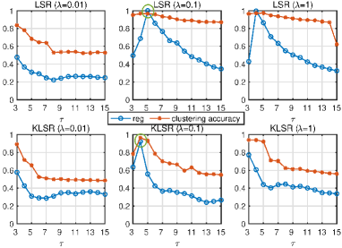
(i) Clustering accuracy and $\textup{reg}(\bm{L})$ (rescaled between 0 and 1) and clustering accuracy of LSR and KLSR on the first 5 subjects of the Extended Yale Face B database.

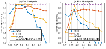
(ii) Clustering accuracies of SSC, LRR, and BDR-B with different hyperparameter $\lambda$ in comparison to AutoSC-GD with LSR and KLSR on the Extended Yale Face B database. The value of $\lambda$ used in BDR-B has been divided by 10. The $\gamma$ in BDR-B is chosen from $\{0.01,0.1,1\}$ and the best one is used for each $\lambda$. In Case (b), the time costs of SSC, LRR, BDR-B, and AutoSC-GD are 9.5s, 33.0s, 7.6s, and 1.6s respectively.

Figure 1: Examples about $\textup{reg}(\bm{L})$, clustering accuracy, and hyperparameters on Extended Yale B.

Now we show the superiority of LSR and KLSR compared to a few important AMC methods. Figure 1(ii) shows the clustering accuracy of SSC (Elhamifar and Vidal, 2013), LRR (Liu et al., 2013), and BDR-B (Lu et al., 2018) with different hyperparameters and our method Auto-GD with LSR and KLSR (detailed by Algorithm 1 in the supplementary material) on the Extended Yale Face B subset. SSC and BDR-B are sensitive to the value of $\lambda$, especially for the relatively difficult task, say Figure 1(ii-b). LRR is not sensitive to the value of $\lambda$ but its accuracy is low. LSR and KLSR are more accurate and efficient than other methods.

The performance of AutoSC-BO

We show the performance of AutoSC-BO with many AMC methods such as SSC (Elhamifar and Vidal, 2013) and LSR. Taking the KLSR model (15) with polynomial kernel as an example, the parameters are $\theta=(\lambda,b,q,\tau)^{\top}$ and the constraints are given by $S=\{\lambda\in\mathbb{R}:\lambda_{min}\leq\lambda\leq\lambda_{max};~{}b\in\mathbb{R}:b_{min}\leq b\leq b_{max};~{}q\in\mathbb{Z}^{+}:q_{min}\leq q\leq q_{max};~{}\tau\in\mathbb{Z}^{+}:\tau_{min}\leq\tau\leq\tau_{max}\}$. More details are in Appendix D.5. Shown in Table 2, larger reg corresponds to higher clustering accuracy and KLSR with polynomial kernel (the optimal $q$ is 1) performs best. Figure 2 shows the performance of KSSC (Patel and Vidal, 2014) and KLSR in each iteration of AutoSC-BO.

Table 2: Clustering accuracy of AutoSC-BO with many methods on Yale Face B dataset (first 10 subjects). All hyperparameters of the kernel functions were optimized via Bayesian optimization.

AMC	$\epsilon$-neigh -borhood	Polynomial kernel	Gaussian kernel	KSSC (Gauss)	KSSC (Poly)	KLSR (Gauss)	KLSR (Poly)
reg${}_{\text{max}}$	0.776	1.294	1.307	0.892	1.388	2.217	2.379
Accuracy	0.325	0.389	0.393	0.584	0.859	0.963	0.966

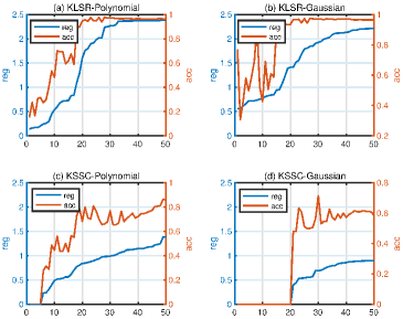
(i) $\text{reg}(\bm{L})$ and clustering accuracy of KLSR and KSSC in each iteration of BO.

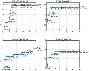
(ii) $\text{reg}(\bm{L})$ and hyperparameters of KLSR and KSSC in each iteration of BO.

Figure 2: AutoSC-BO with KSSC and KLSR on the first 10 subjects of YaleB Face dataset.

Relative-Eigen-Gap versus Eigen-Gap

We compare the proposed relative-eigen-gap (reg$(\mathbf{L})$) with eigen-gap (denoted by eg$(\mathbf{L})$), and the regularizer J$(\mathbf{L},\alpha)$ proposed by (Meila and Shortreed, 2006) with different $\alpha$. Note that in AutoSC, we need to minimize J$(\mathbf{L},\alpha)$ instead. The clustering results of AutoSC-GD are reported in Table 3 (details about the datasets are in Section 4). We see that our reg$(\mathbf{L})$ outperforms eg$(\mathbf{L})$ and J$(\mathbf{L},\alpha)$ in all cases except AR.

Table 3: The comparison of AutoSC-GD with reg$(\mathbf{L})$, eg$(\mathbf{L})$, and J$(\mathbf{L},\alpha)$

	YaleB	ORL	COIL20	AR	MNIST	F-MNIST
eg$(\mathbf{L})$	0.790	0.768	0.619	0.805	0.663	0.562
J$(\mathbf{L},0$)	0.823	0.795	0.750	0.804	0.726	0.516
J$(\mathbf{L},-0.1$)	0.818	0.788	0.768	0.826	0.718	0.519
J$(\mathbf{L},-1$)	0.812	0.785	0.769	0.817	0.722	0.523
J$(\mathbf{L},-10$)	0.804	0.788	0.768	0.832	0.731	0.539
J$(\mathbf{L},-100$)	0.788	0.765	0.769	0.817	0.735	0.545
reg$(\mathbf{L})$	0.897	0.795	0.782	0.786	0.755	0.595

4.2 Comparative studies of AutoSC and baselines

First we compare AutoSC with SSC, LRR (Liu et al., 2013), LSR (Lu et al., 2012), EDSC (Pan Ji et al., 2014), KSSC, SSC-OMP (You et al., 2016b), BDR-Z (Lu et al., 2018), and BDR-B (Lu et al., 2018) on six smaller datasets. The clustering accuracy and time cost are reported in Table 4. AutoSC-GD and AutoSC-BO outperformed other methods significantly in almost all cases. SSC-OMP and AutoSC-GD are more efficient than SSC, LRR, EDSC, and KSSC. The time cost of AutoSC-BO is much higher than that of AutoSC-GD because the former optimizes all hyperparameters including $\lambda$, $\tau$, and kernel parameters (e.g. $b,q$).

Table 4: Clustering performance on the six small datasets. For the MNIST-1k and Fahsion-MNIST-1k, we report the average results of 20 trials because the subset is formed randomly. AutoSC chose LSR for Yale B and AR and chose KLSR for others datasets. The NMI results are in Table 7 (See Appendix D.3).

		SSC	LRR	LSR	EDSC	KSSC	SSC-OMP	BDR-Z	BDR-B	AutoSC-GD	AutoSC-BO
Yale B	acc	0.723	0.643	0.592	0.806	0.649	0.768	0.596	0.719	0.897	0.909
	time	273.8	928.1	7.3	58.6	464.3	8.9	368.8	368.8	19.1	78.3
ORL	acc	0.711	0.762	0.680	0.712	0.707	0.665	0.739	0.735	0.795	0.803
	time	2.7	8.8	0.5	2.0	2.6	0.4	3.9	3.9	2.3	20.5
COIL20	acc	0.871	0.729	0.695	0.759	0.912	0.658	0.713	0.791	0.782	0.878
	time	61.8	221.2	1.4	15.4	100.6	2.5	86.8	86.8	7.6	39.2
AR	acc	0.718	0.769	0.665	0.673	0.726	0.669	0.745	0.751	0.786	0.826
	time	317.5	1220.6	14.5	69.1	627.4	57.6	578.7	578.7	43.4	130.6
MNIST -1k	acc	0.596 (0.054)	0.513 (0.037)	0.554 (0.041)	0.536 (0.035)	0.577 (0.053)	0.542 (0.038)	0.576 (0.037)	0.578 (0.043)	0.615 (0.041)	0.619 (0.038)
	time	24.9	69.1	0.8	5.2	32.8	1.3	26.9	26.9	2.5	21.7
Fashion- MNIST-1k	acc	0.553 (0.025)	0.515 (0.014)	0.563 (0.023)	0.544 (0.017)	0.548 (0.016)	0.566 (0.034)	0.574 (0.019)	0.563 (0.031)	0.581 (0.025)	0.584 (0.021)
	time	24.1	68.5	0.7	5.1	35.9	1.2	25.7	25.7	2.6	22.7

We compare our method with LSR, LSC-K (Chen and Cai, 2011), SSC-OMP (You et al., 2016b), and S⁵C (Matsushima and Brbic, 2019), and S³COMP-C (Chen et al., 2020) on the larger datasets. The parameter settings are in Appendix D.6. Table 5 shows the clustering accuracy and standard deviation of 10 repeated trials on the raw-pixel data of MNIST and Fashion-MNIST. Table 6 shows the results on MNIST and Fashion-MNIST features and GTSRB. Our methods have the highest clustering accuracy in every case. Note that if NSE is ablated, the accuracy of AutoSC-GD on MNIST(features)-10k, -20k, and -30k are 0.9772, 0.9783 and 0.9864 respectively, higher than those of AutoSC-GD+NSE, though the time costs increased.

It is worth mentioning that, to the best of our knowledge, the deep clustering method of (Zhang et al., 2019a) has SOTA performance on Yale B (acc=0.98) and ORL (acc=0.89), the method proposed by (Zhang et al., 2019b) has SOTA performance on Fashion-MNIST (acc=0.72), the method proposed by (Mahon and Lukasiewicz, 2021) has SOTA performance on MNIST (acc=0.99), and our method has SOTA performance on GTSRB. Nevertheless, we focus on automated spectral clustering.

Table 5: Clustering accuracy and time cost (second) on MNIST and Fashion MNIST. “—” means the computation is out of memory.

		LSR	LSC-K	SSC-OMP	S5C	S3COMP-C	AutoSC-GD+NSE	AutoSC-BO+NSE
MNIST-10k	acc	0.583(0.007)	0.652(0.037)	0.431(0.014)	0.646(0.045)	0.623(0.028)	0.687(0.035)	0.679(0.034)
	time	154.9	18.9	26.4	82.3	710.4/20	16.2	48.3
MNIST	acc	—	0.665(0.021)	0.453(0.017)	0.627(0.025)	—	0.755(0.022)	0.750(0.009)
	time	—	329.2	1178.3	961.5	—	86.9	123.6
Fashion- MNIST-10k	acc	0.561(0.008)	0.571(0.025)	0.509(0.038)	0.565(0.021)	0.569(0.024)	0.576(0.011)	0.572(0.019)
	time	153.6	18.6	26.8	107.3	707.2/20	17.3	50.9
Fashion- MNIST	acc	—	0.561(0.015)	0.359(0.017)	0.559(0.013)	—	0.586(0.008)	0.578(0.012)
	time	—	335.1	1156.6	932.6	—	88.7	122.8

Table 6: Clustering accuracy (mean value and standard deviation) and time cost (second) on MNIST and Fashion-MNIST with feature extraction. “/” means the algorithm was performed on a computational platform not comparable to ours. The underlined values are from (Chen et al., 2020).

		LSC-K	SSC-OMP	S5C	S3COMP-C	AutoSC-GD+NSE	AutoSC-BO+NSE
MNIST	acc	0.8659(0.0215)	0.8159	0.7829(0.0283)	0.9632	0.9775(0.0034)	0.9741(0.0044)
	time	273.6	280.6	907.5	416.8	59.2	115.3
Fashion- MNIST	acc	0.6131(0.0298)	0.3796(0.0217)	0.6057(0.0227)	—	0.6398(0.0133)	0.6461(0.0104)
	time	251.8	1013.9	913.2	—	61.9	112.6
GTSRB	acc	0.8711(0.0510)	0.8252	0.9044(0.0267)	0.9554	0.9873(0.0126)	0.9881(0.0078)
	time	31.2	/	98.7	/	16.8	69.4

5 Conclusion

We have proposed an automated spectral clustering method. Extensive experiments showed the effectiveness and superiority of our methods over baseline methods. The efficiency improvement is from the closed-form solutions of the least squares regressions. The accuracy improvement is from the effectiveness of LSR and KLSR with thresholding and the automation of model and hyperparameter selection. One limitation of this work is that we only considered automated spectral clustering while there are many other clustering methods (e.g. (Fan, 2021)) not relying on affinity matrix.

Checklist

The checklist follows the references. Please read the checklist guidelines carefully for information on how to answer these questions. For each question, change the default [TODO] to [Yes] , [No] , or [N/A] . You are strongly encouraged to include a justification to your answer, either by referencing the appropriate section of your paper or providing a brief inline description. For example:

• Did you include the license to the code and datasets? [Yes] See Section.

• Did you include the license to the code and datasets? [No] The code and the data are proprietary.

• Did you include the license to the code and datasets? [N/A]

Please do not modify the questions and only use the provided macros for your answers. Note that the Checklist section does not count towards the page limit. In your paper, please delete this instructions block and only keep the Checklist section heading above along with the questions/answers below.

1. For all authors…

   1. Do the main claims made in the abstract and introduction accurately reflect the paper’s contributions and scope? [Yes]

   2. Did you describe the limitations of your work? [N/A]

   3. Did you discuss any potential negative societal impacts of your work? [N/A]

   4. Have you read the ethics review guidelines and ensured that your paper conforms to them? [Yes]

2. If you are including theoretical results…

   1. Did you state the full set of assumptions of all theoretical results? [Yes]

   2. Did you include complete proofs of all theoretical results? [Yes]

3. If you ran experiments…

   1. Did you include the code, data, and instructions needed to reproduce the main experimental results (either in the supplemental material or as a URL)? [Yes]

   2. Did you specify all the training details (e.g., data splits, hyperparameters, how they were chosen)? [Yes]

   3. Did you report error bars (e.g., with respect to the random seed after running experiments multiple times)? [Yes]

   4. Did you include the total amount of compute and the type of resources used (e.g., type of GPUs, internal cluster, or cloud provider)? [Yes]

4. If you are using existing assets (e.g., code, data, models) or curating/releasing new assets…

   1. If your work uses existing assets, did you cite the creators? [Yes]

   2. Did you mention the license of the assets? [N/A]

   3. Did you include any new assets either in the supplemental material or as a URL? [N/A]

   4. Did you discuss whether and how consent was obtained from people whose data you’re using/curating? [N/A]

   5. Did you discuss whether the data you are using/curating contains personally identifiable information or offensive content? [N/A]

5. If you used crowdsourcing or conducted research with human subjects…

   1. Did you include the full text of instructions given to participants and screenshots, if applicable? [N/A]

   2. Did you describe any potential participant risks, with links to Institutional Review Board (IRB) approvals, if applicable? [N/A]

   3. Did you include the estimated hourly wage paid to participants and the total amount spent on participant compensation? [N/A]

Appendix A More discussion about LSR and KLSR

Note that if $n\ll m$, using the push-through identity [Henderson and Searle, 1981], we reformulate $\bm{C}=(\bm{X}^{\top}\bm{X}+\lambda\bm{I})^{-1}\bm{X}^{\top}\bm{X}$ as $\bm{C}=\bm{X}^{\top}(\lambda\bm{I}+\bm{X}\bm{X}^{\top})^{-1}\bm{X}$ to reduce the computational cost from $O(n^{3})$ to $O(mn^{2})$. In $\bm{C}=(\bm{K}+\lambda\bm{I})^{-1}\bm{K}$, when $n$ is large (e.g.$>5000$), we perform randomized SVD [Halko et al., 2011] on $\bm{K}$: $\bm{K}\approx\bm{V}_{r}\bm{\Sigma}_{r}\bm{V}_{r}^{\top}$. Then $\bm{C}\approx\bm{V}_{r}\bm{\Sigma}_{r}^{1/2}(\lambda\bm{I}+\bm{\Sigma})^{-1}\bm{\Sigma}_{r}^{1/2}\bm{V}_{r}^{\top}$, where $r=20k$ works well in practical applications. The time complexity of computing $\bm{C}$ is $O(r\tau n+rn^{2})$. The computation of the smallest $k+1$ eigenvalues of $\bm{L}$ is equivalent to compute the largest $k+1$ eigenvalues and eigenvectors of $\bm{D}^{-1/2}\bm{A}\bm{D}^{-1/2}$, which is sparse. The time complexity is $O(k\tau n)$. We have the following result.

Proposition A.1.

Let $\hat{\bm{c}}$ be the optimal solution of $\mathop{\textup{minimize}}_{\bm{c}}\tfrac{1}{2}\|\phi(\bm{y})-\phi(\bm{X})\bm{c}\|^{2}+\tfrac{\lambda}{2}\|\bm{c}\|^{2}$, where $\phi$ is induced by Gaussian kernel and $\bm{y}$ is arbitrary. Then $\|\hat{c}_{i}-\hat{c}_{j}\|\leq\sqrt{2-2\exp\left(-\|\bm{x}_{i}-\bm{x}_{j}\|^{2}/(2\varsigma^{2})\right)}$.

It shows that when two data points in $\bm{X}$, e.g. $\bm{x}_{i}$ and $\bm{x}_{j}$, are close to each other, the corresponding two elements in $\hat{\bm{c}}$, e.g. $\hat{c}_{i}$ and $\hat{c}_{j}$, have small difference. Hence KLSR with Gaussian kernel utilizes local information to enhance $\bm{C}$.

In LSR and KLSR, let $\lambda\in{\Lambda}$, $\tau\in\mathcal{T}$, and $\Theta={\Lambda}\times\mathcal{T}$. The algorithm of AutoSC-GD with only LSR and KLSR is shown in Algorithm 1. The total time complexity is

$$O\left(|\Lambda|(mn^{2}+r\bar{\tau}n+rn^{2})+2|\Lambda||\mathcal{T}|k\bar{\tau}n\right),$$

where $\bar{\tau}$ denotes the mean value in $\mathcal{T}$. The time complexity is at most $O(|\Lambda|\left(mn^{2}+|\mathcal{T}|kmn)\right)$ when $\tau\leq r\leq m\leq n$. It is worth noting that Algorithm 1 can be easily implemented parallelly, which will reduce the time complexity to $O(\max(m,r)n^{2}+kmn)$. On the contrary, SSC, LRR, and their variants require iterative optimization and hence their time complexity is about $O(tmn^{2})$, where $t$ denotes the iteration number and is often larger than $100$.

Algorithm 1 AutoSC-GD with Only LSR and KLSR

0:  $\bm{X}$, $k$, $\mathcal{F}$, $\Lambda$, $\mathcal{T}$

1:  Normalize the columns of $\bm{X}$ to have unit $\ell_{2}$ norm.

2:  for $f_{u}$ in $\mathcal{F}$ do

3:     for $\lambda_{i}$ in $\Lambda$ do

4:        Construct $\bm{C}$ by (13) or (15).

5:        for $\tau_{j}$ in $\mathcal{T}$ do

6:           $\bm{C}\leftarrow|\bm{C}\odot(\bm{1}-\bm{I})|$.

7:           Truncate $\bm{C}$ with parameter $\tau_{j}$.

8:           For $j=1,\ldots,n$, let $\bm{c}_{j}\leftarrow\bm{c}_{j}/|\bm{c}_{j}|_{1}$.

9:           $\bm{A}=(\bm{C}+\bm{C}^{\top})/2$.

10:           $\bm{L}=\bm{I}-\bm{D}^{-1/2}\bm{A}\bm{D}^{-1/2}$.

11:           Compute $\sigma_{1},\ldots,\sigma_{k+1}$ and $\bm{v}_{1},\ldots,\bm{v}_{k}$.

12:           $\Delta_{uij}=\textup{REG}(\bm{L})$, $\mathcal{V}_{uij}=[\bm{v}_{1},\ldots,\bm{v}_{k}]$.

13:        end for

14:     end for

15:  end for

16:  $\bm{Z}=\mathcal{V}_{\bar{u}\bar{i}\bar{j}}^{\top}$, where $\{\bar{u},\bar{i},\bar{j}\}=\textup{argmax}_{u,i,j}\Delta_{uij}$.

17:  Normalize the columns of $\bm{Z}$ to have unit $\ell_{2}$ norm.

18:  Perform k-means on $\bm{Z}$.

18:  $k$ clusters: $C_{1},\ldots,C_{k}$.

Appendix B The algorithm of AutoSC+NSE

See Algorithm 2.

Algorithm 2 AutoSC+NSE

0:  $\bm{X}$, $k$, $\mathcal{F}$, $\Theta$, $\hat{n}$.

1:  Select $\hat{n}$ landmarks from $\bm{X}$ by k-means to form $\hat{\bm{X}}$.

2:  Apply AutoSC-GD or AutoSC-BO to $\hat{\bm{X}}$ with $\mathcal{F}$ and $\Theta$.

2:  Get $\hat{\bm{Z}}$ from the best Laplacian matrix given by AutoSC-G or AutoSC-BO.

3:  Use mini-batch Adam to solve (17).

4:  Compute $\bm{Z}$ by (18).

5:  Perform k-means on $\bm{Z}$.

5:  $k$ clusters: $C_{1},\ldots,C_{k}$.

Appendix C More theoretical results

C.1 Theoretical guarantee for KLSR

Definition C.1 (Polynomial Deterministic Model).

The columns of $\bm{X}_{0}\in\mathbb{R}^{m\times n}$ are drawn from a union of $k$ different polynomials $\{g_{j}:\mathbb{R}^{r}\rightarrow\mathbb{R}^{m},~{}r<m\}_{j=1}^{k}$ of order at most $p$ and are further corrupted by noise, say $\bm{X}=\bm{X}_{0}+\bm{E}$. Denote the eigenvalue decomposition of the kernel matrix $\bm{K}$ of $\bm{X}$ as $\bm{K}=\bm{V}\bm{\Sigma}\bm{V}^{\top}$, where $\bm{\Sigma}=\textup{diag}(\sigma_{1},\ldots,\sigma_{n})$ and $\sigma_{1}\geq\sigma_{2}\geq\cdots\sigma_{n}$. Let $\gamma=\sigma_{d+1}/\sigma_{d}$. Denote $\bm{v}_{i}=(v_{i1},\ldots,v_{in})$ the $i$-th row of $\bm{V}$ and let $\bar{\bm{v}}_{i}=(v_{i1},\ldots,v_{id})$, where $d<n$. Suppose the following conditions hold: 1) for every $i\in[n]$, the $\bar{\tau}$-th largest element of $\{|\bar{\bm{v}}_{i}^{\top}\bar{\bm{v}}_{j}|:j\in C_{\pi(i)}\}$ is greater than $\alpha$; 2) $\max_{i\in[n]}\max_{j\in[n]\setminus C_{\pi(i)}}|\bar{\bm{v}}_{i}^{\top}\bar{\bm{v}}_{j}|\leq\beta$; 3) $\max_{i,j,l}|v_{il}v_{jl}|\leq\mu$.

Here we consider polynomials because they are easy to analyze and can well approximate smooth functions provided that $p$ is sufficiently large. Clustering the columns of $\bm{X}$ given by Definition C.1 according to the polynomials is actually a manifold clustering problem beyond the setting of subspace clustering. Similar to the subspace detection property, we define

Definition C.2 (Manifold Detection Property).

A symmetric affinity matrix $\bm{A}$ obtained from $\bm{X}$ has manifold detection property if for all $i$, the nonzero elements of $\bm{a}_{i}$ correspond to the columns of $\bm{X}$ lying on the same manifold as $\bm{x}_{i}$.

The following theorem verifies the effectiveness of (15) followed by the truncation operation in manifold detection.

Theorem C.3.

Suppose $\bm{X}$ and $\bm{K}$ are given by Definition C.1 and $\bm{C}$ is given by (15), where the kernel function is a polynomial kernel of order $q$, $\textup{rank}(\bm{K}_{0})=d$ ($\bm{K}_{0}$ is from $\bm{X}_{0}$), and

$$\tfrac{\left(\rho-\sqrt{\rho^{2}-4(2\mu d-\Delta)(2\mu n-2\mu d-\Delta)}\right)\sigma_{d}^{2}}{4\mu d-2\Delta}<\lambda<\tfrac{\left(\rho+\sqrt{\rho^{2}-4(2\mu d-\Delta)(2\mu n-2\mu d-\Delta)}\right)\sigma_{d}^{2}}{4\mu d-2\Delta}$$ (19)

where $\rho=2\mu n\gamma^{2}-\Delta(1+\gamma^{2})$. Then $d\leq k\binom{r+pq}{pq}$ and the $\bm{C}$ truncated by $\tau\leq\bar{\tau}$ has the manifold detection property.

In the theorem, $\sigma_{d}$ can be much larger than $\sigma_{d+1}$ provided that the noise is small enough. Then we get a wide range for $\lambda$. Compared to Theorem 3.7, Theorem C.3 allows a much larger $d$, which means the kernel method is able to handle more difficult clustering problems than the linear method.

C.2 Theoretical analysis for NSE

The following proposition shows that a small number of hidden nodes in NSE are sufficient to make the clustering succeed.

Proposition C.4.

Suppose the columns (with unit $\ell_{2}$ norm) of $\bm{X}$ are drawn from a union of $k$ independent subspaces of dimension $r$: $\sum_{j=1}^{k}\textup{dim}(\mathcal{S}_{j})=\textup{dim}(\mathcal{S}_{1}\cup\cdots\cup\mathcal{S}_{k})=kr$. For $j=1,\ldots,k$, let $\bm{U}^{j}$ be the bases of $\mathcal{S}_{j}$ and $\bm{x}_{i}=\bm{U}^{j}\bm{v}_{i}$, if $\bm{x}_{i}\in\mathcal{S}_{j}$. Suppose $\max\{\|{\bm{U}_{:l}^{i}}^{\top}\bm{U}^{j}\|:1\leq l\leq r,1\leq i\neq j\leq k\}\leq\mu$. Suppose that for all $i=1,\ldots n$, $\max\{v_{1i},\ldots,v_{ri}\}>\mu$. Then there exist $\bm{W}_{1}\in\mathbb{R}^{d\times m}$, $\bm{W}_{2}\in\mathbb{R}^{k\times d}$, $\bm{b}_{1}\in\mathbb{R}^{d}$, and $\bm{b}_{2}\in\mathbb{R}^{k}$ such that performing k-means on $\bm{Z}$ given by (18) identifies the clusters correctly, where $d=kr$.

Appendix D More about the experiments

D.1 Dataset description

The description for the benchmark image datasets considered in this paper are as follows.

• Extended Yale B Face [Kuang-Chih et al., 2005] (Yale B for short): face images (192$\times$168) of 38 subjects. Each subject has about 64 images under various illumination conditions. We resize the images into $32\times 32$.

• ORL Face [Samaria and Harter, 1994]: face images (112$\times$92) of 40 subjects. Each subject has 10 images with different poses and facial expressions. We resize the images into 32$\times$32.

• COIL20 [Nene et al., 1996]: images ($32\times 32$) of 20 objects. Each object has 72 images of different poses.

• AR Face [Martínez and Kak, 2001]: face images (165$\times$120) of 50 males and 50 females. Each subject has 26 images with different facial expressions, illumination conditions, and occlusions. We resize the images into $42\times 30$.

• MNIST [LeCun et al., 1998]: 70,000 grey images ($28\times 28$) of handwritten digits $0-9$.

• MNIST-1k(10k): a subset of MNIST containing 1000(10000) samples, 100(1000) randomly selected samples per class.

• Fashion-MNIST [Xiao et al., 2017]: 70,000 gray images ($28\times 28$) of 10 types of fashion product.

• Fashion-MNIST-1k(10k): a subset of Fashion-MNIST containing 1000(10000) samples, 100(1000) randomly selected samples per class.

• MNIST-feature: following the same procedures of [Chen et al., 2020], we compute a feature vector of dimension 3,472 using the scattering convolution network [Bruna and Mallat, 2013] and then reduce the dimension to 500 using PCA.

• Fashion-MNIST-feature: similar to MNIST-feature.

• GTSRB [Stallkamp et al., 2012]: consisting of 12,390 images of street signs in 14 categories. Following [Chen et al., 2020], we extract a 1568-dimensional HOG feature, and reduce the dimension to 500 by PCA.

All experiments are conducted in MATLAB on a MacBook Pro with 2.3 GHz Intel i5 Core and 8GB RAM.

D.2 Hyperparameter settings for the small datasets

We select $\lambda$ from $\{0.01,0.02,0.05,0.1,0.2,\ldots,0.5\}$ for SSC, LRR, and KSSC. The $\lambda$ in BDR is chosen from $\{5,10,20,\ldots,80\}$. The $\gamma$ in BDR-B and BDR-Z is chosen from $\{0.01,0.1,1\}$. The parameter $s$ in SSC-OMP is chosen from $\{3,4,\ldots,15\}$. We report the results of these methods with their best hyperparameters. In AutoSC, we set $\Lambda=\{0.01,0.1,1\}$ and $\mathcal{T}=\{5,6,\ldots,15\}$. In AutoSC-BO, we consider two models: 1) Gaussian kernel similarity; 2) KLSR with polynomial kernel; 3) KLSR with Gaussian kernel, in which the hyperparameters of kernels are optimized adaptively. Then we needn’t to consider LSR explicitly because it is a special case of KLSR with polynomial kernel. See Appendix D.5.

D.3 Clustering results in terms of NMI

In addition to the clustering accuracy reported in Table 4, here we also compare the normalized mutual information (NMI) in Table 7. We see that the comparative performance of all methods are similar to the results in Table 4 and our methods AutoSC-GD and AutoSC-BO outperformed other methods in almost all cases.

Table 7: Normalized Mutual Information on the six small datasets

	SSC	LRR	EDSC	KSSC	SSC-OMP	BDR-Z	BDR-B	AutoSC-GD	AutoSC-BO
Yale B	0.817	0.703	0.835	0.730	0.841	0.666	0.743	0.919	0.928
ORL	0.849	0.872	0.856	0.872	0.815	0.875	0.865	0.907	0.903
COIL20	0.954	0.706	0.843	0.983	0.671	0.843	0.873	0.897	0.963
AR	0.818	0.872	0.825	0.809	0.691	0.865	0.861	0.887	0.904
MNIST-1k	0.612	0.538	0.631	0.626	0.546	0.634	0.580	0.667	0.652
Fashion-MNIST-1k	0.616	0.601	0.621	0.621	0.559	0.614	0.605	0.633	0.629

D.4 The stability of AutoSC

Though we have used a relatively compact search space in AutoSC to reduce the highly unnecessary computational cost, the search space can be arbitrarily large. Figure 3 shows the clustering accuracy and the corresponding relative-eigen-gap. We can see that the region with highest relative-eigen-gap is in accordance with the region with highest clustering accuracy.

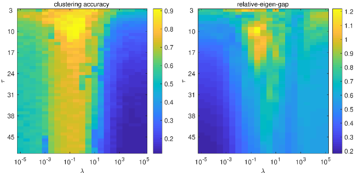
Figure 3: Visualization of the clustering accuracy and the corresponding relative-eigen-gap when a large search space is used.

D.5 More about AutoSC-BO in the experiments

For SSC, we consider the following problem

$$\mathop{\textup{minimize}}_{\bm{C}}\ \tfrac{1}{2}\textup{Tr}\left(\bm{K}-2\bm{K}\bm{C}+\bm{C}^{\top}\bm{K}\bm{C}\right)+{\lambda}\|\bm{C}\|_{1},$$ (20)

where $\bm{K}$ is an $n\times n$ kernel matrix with $[\bm{K}]_{ij}=k(\bm{x}_{i},\bm{x}_{j})$. Note that when we use a linear kernel function, (20) reduces to the vanilla SSC. We solve the optimization via alternating direction method of multipliers (ADMM) [Boyd et al., 2011], where the Lagrange parameter is 0.1 and the maximum number of iterations is 500. In this study, we consider polynomial kernel and Gaussian kernel, and optimize all hyperparameters including the order of the polynomial kernel. Particularly, for Gaussian kernel, we set $\varsigma=\frac{\xi}{n^{2}}\sum_{ij}\|\bm{x}_{i}-\bm{x}_{j}\|$ and optimize $\xi$. The search space for the hyperparameters are as follows: $10^{-3}\leq\lambda\leq 1$, $5\leq\tau\leq 50$, $0\leq b\leq 10^{3}$, $1\leq q\leq 5$, $0.5\leq\xi\leq 5$.

In addition to Figure 2 of the main paper, here we report the best hyperparameters of the four models found by AutoSC-BO in Table 8. It can be found that the accuracy of KLSR with a linear kernel is higher than other models, which is consistent with its highest reg.

Table 8: The best hyperparameters and the corresponding clustering accuracy given by AutoSC_BO on the first 10 subjects of YaleB Face dataset.

method	hyperparameters	reg	accuracy
KLSR (Polynomial)	$\lambda=0.207$, $b=19.09$, $q=1$, $\tau=5$	2.379	0.966
KLSR (Gaussian)	$\lambda=0.013$, $\xi=4.92$, $\tau=5$	2.217	0.963
KSSC (Polynomial)	$\lambda=0.519$, $b=44.57$, $q=2$, $\tau=5$	1.388	0.859
KSSC (Gaussian)	$\lambda=0.0011$, $\xi=4.97$, $\tau=6$	0.892	0.584

D.6 Hyperparameter settings of large-scale clustering

On MNIST-10k, MNIST, Fashion-MNIST-10k, and Fashion-MNIST, the parameter settings of [Chen and Cai, 2011], SSSC [Peng et al., 2013], SSC-OMP [You et al., 2016b], and S⁵C [Matsushima and Brbic, 2019], and S³COMP-C [Chen et al., 2020], and AutoSC+NSE are shown in Table 9. These hyper parameters have been determined via grid search and the best (as possible) values are used.

Table 9: Hyper-parameter settings of the compared methods on MNIST-10k, MNIST, Fashion-MNIST-10k, and Fashion-MNIST. $s$ denotes the number of landmark data points. In the optimization (mini-batch Adam) of AutoSC+NSE, the epoch number, batch size, and step size are 200, 128, and $10^{-3}$ respectively.

LSC-K	$s=1000$, $r=3$
SSSC	$s=1000$, $\lambda=0.01$
SSC-OMP	$K=10$ (sparsity)
S5C	$s=1000$, $\lambda=0.1$ or $0.2$
S3COMP-C	$T=20$, $\lambda=0.4$, $\delta=0.9$
AutoSC+NSE	$s=1000$, $d=200$, $\gamma=10^{-5}$
AutoSCBO+NSE	$s=1000$, $d=200$, $\gamma=10^{-5}$

D.7 Influence of hyper-parameters in AutoSC+NSE

We investigate the effects of the type of activation function and the number ($d$) of nodes in the hidden layer of NSE. For convenience, we used a fixed random seed of MATLAB (rng(1)). Figure 4 shows the clustering accuracy on MNIST given by AutoSC+NSE with different activation function and different $d$. We see that ReLU outperformed tanh consistently. The reason is that the nonlinear mapping $g$ from the data space to the eigenspace of the Laplacian matrix is nonsmooth and ReLU is more effective than tanh in approximating nonsmooth functions. In addition, when $d$ increases, the clustering accuracy of AutoSC+NSE with ReLU often becomes higher because a wider network often has a higher ability of function approximation.

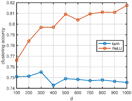
Figure 4: ReLU v.s. tanh (hyperbolic tangent) in the hidden layer of AutoSC+NSE on MNIST. When using ReLU, we set $\gamma=10^{-5}$ and $\alpha=10^{-3}$ (the step size in Adam). When using tanh, we set $\gamma=10^{-3}$ and $\alpha=10^{-2}$, which perform best in this case. Notice that the clustering accuracy when using ReLU is higher than 0.78 in almost all cases, which is higher than the value (say $0.755$) we reported in the main paper. The reason is that in the main paper, we reported the mean value of 10 repeated trials but here we report the value of a single trial.

Figure 5 shows the clustering accuracy on MNIST given by AutoSC+NSE with different $\gamma$ and $\alpha$. When $\alpha$ is too small (say $10^{-4}$, the clustering accuracy is low, because the training error is quite large in 200 epochs. In fact, by increasing the training epochs, the clustering accuracy can be improved, which however will increase the time cost. When $\alpha$ is relatively large, the clustering accuracy is often higher than 0.755. On the other hand, AutoSC+NSE is not sensitive to $\gamma$ provided that it is not too large.

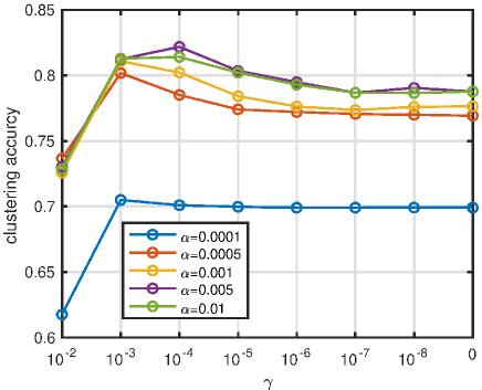
Figure 5: Influence of $\gamma$ and $\alpha$ in AutoSC+NSE on MNIST. We set $d=200$ and use ReLU.

Figure 6 shows the mean value and standard deviation (10 repeated trials) of the clustering accuracy on MNIST given by AutoSC+NSE with different number (denoted by $s$) of landmark points. It can be found that when the $s$ increases, the clustering accuracy increases and its standard deviation becomes smaller. When $s$ is large enough, the improvement is not significant.

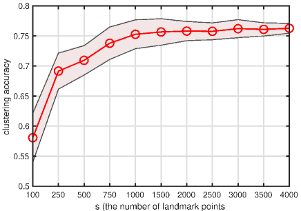
Figure 6: Influence of the number of landmark points in AutoSC+NSE on MNIST. We set $d=200$, $\gamma=10^{-5}$, and $\alpha=10^{-3}$. The shadow denotes the standard deviation of 10 trials.

Appendix E Proof for the theoretical results

E.1 Proof for Claim 3.2

Proof.

The stochastic transition matrix of $G$ is defined as

$$\bm{P}=\bm{D}^{-1}\bm{A}.$$ (21)

In [Meila, 2001], it was showed that

$$\textup{MNCut}(\mathcal{C})\geq k-\sum_{i=1}^{k}\varrho_{i}(\bm{P}),$$ (22)

where $\varrho_{i}(\bm{P})$ denotes the $i$-th largest eigenvalue of $\bm{P}$ and $1=\varrho_{1}(\bm{P})\geq\varrho_{2}(\bm{P})\geq\cdots\varrho_{k}(\bm{P})$. According to Lemma 3 of [Meila, 2001], we have

$$\sigma_{i}(\bm{L})=1-\varrho_{i}(\bm{P}),\quad\forall i=1,\ldots,n.$$ (23)

Substituting (23) into (22), we have

$$\textup{MNCut}(\mathcal{C})\geq\sum_{i=1}^{k}\sigma_{i}(\bm{L}).$$ (24)

∎

Remark E.1.

$\mathcal{C}$ can be any partition of the nodes of $G$. Let $\mathcal{C}^{\ast}$ be the optimal partition. Then $\textup{MNCut}(\mathcal{C}^{\ast})=\sum_{i=1}^{k}\sigma_{i}(\bm{L})$. If $\sum_{i=1}^{k}\sigma_{i}(\bm{L})=0$, there are no connections (edges) among $C_{1}^{\ast},\ldots,C_{k}^{\ast}$.

E.2 Proof for Claim 3.3

Proof.

For $i=1,\ldots,k$, we aim to partition $C_{i}$ into two subsets, denoted by $C_{i}^{1}$ and $C_{i}^{2}$. Then we define

$$\textup{MNCut}(C_{i})=\dfrac{Cut(C_{i}^{1},C_{i}^{2})}{Vol(C_{i}^{1})}+\dfrac{Cut(C_{i}^{2},C_{i}^{1})}{Vol(C_{i}^{2})}.$$ (25)

It follows that

$$\textup{MNCut}(C_{i})\geq\sum_{j=1}^{2}\sigma_{j}(\bm{L}_{C_{i}})\geq\sigma_{2}(\bm{L}_{C_{i}})=ac(C_{i}),$$ (26)

where $\bm{L}_{C_{i}}$ denotes the Laplacian matrix of $C_{i}$ an $i=1,\ldots,k$. Since $\sigma_{k+1}(\bm{L})=\min\{ac(C_{1}),\ldots,ac(C_{k})\}$, we have

$$\min_{1\leq i\leq k}\textup{MNCut}(C_{i})\geq\sigma_{k+1}(\bm{L}).$$ (27)

Therefore, $\sigma_{k+1}(\bm{L})$ measures the least connectivity of $C_{1},\ldots,C_{k}$. This finished the proof. ∎

Remark E.2.

When $\sigma_{k+1}(\bm{L})$ is large, the connectivity in each of $C_{1},\ldots,C_{k}$ is strong. Otherwise, the connectivity in each of $C_{1},\ldots,C_{k}$ is weak. When $\sigma_{k+1}(\bm{L})=0$, at least one of $C_{1},\ldots,C_{k}$ contains at least two components, which means the nodes of $G$ can be partitioned into $k+1$ or more clusters.

E.3 Proof for Theorem 3.4

Proof.

According to Theorem 1 of [Meila et al., 2005], we have

$$\textup{dist}(\mathcal{C},\mathcal{C}^{\prime})<\dfrac{3\delta}{\sigma_{k+1}(\bm{L})-\sigma_{k}(\bm{L})}.$$ (28)

Since $\textup{reg}(\bm{L})=\dfrac{\sigma_{k+1}(\bm{L})-\frac{1}{k}\sum_{i=1}^{k}\sigma_{i}(\bm{L})}{\frac{1}{k}\sum_{i=1}^{k}\sigma_{i}(\bm{L})+\epsilon}$, we have

$$\sigma_{k+1}(\bm{L})-\sigma_{k}(\bm{L})=\textup{reg}(\bm{L})(\bar{\sigma}+\epsilon)+\bar{\sigma}-\sigma_{k}(\bm{L}),$$ (29)

where $\bar{\sigma}=\frac{1}{k}\sum_{i=1}^{k}\sigma_{i}(\bm{L})\geq\epsilon$. Invoking (29) into (28), we arrive at

$$\textup{dist}(\mathcal{C},\mathcal{C}^{\prime}) <\dfrac{3\delta}{\textup{reg}(\bm{L})(\bar{\sigma}+\epsilon)+\bar{\sigma}-\sigma_{k}(\bm{L})}$$

$$\leq\dfrac{3\delta}{2\epsilon\textup{reg}(\bm{L})+\bar{\sigma}-k\bar{\sigma}}$$

$$\leq\dfrac{3\delta}{2\epsilon\textup{reg}(\bm{L})+(1-k)\eta\epsilon}$$

$$\leq\dfrac{1.5\delta\epsilon^{-1}}{\textup{reg}(\bm{L})+(1-k)\eta/2}.$$

This finished the proof. ∎

E.4 Proof for Proposition A.1

Proof.

Since $\hat{\bm{c}}$ is the optimal solution, we have

$$\phi(\bm{x}_{i})^{\top}\left(\phi(\bm{y})-\phi(\bm{X})\hat{\bm{c}}\right)+\lambda\hat{c}_{i}=0,$$

$$\phi(\bm{x}_{j})^{\top}\left(\phi(\bm{y})-\phi(\bm{X})\hat{\bm{c}}\right)+\lambda\hat{c}_{j}=0.$$

It follows that

$$\|\hat{c}_{i}-\hat{c}_{j}\| =\|\left(\phi(\bm{x}_{i})-\phi(\bm{x}_{j})\right)^{\top}\left(\phi(\bm{y})-\phi(\bm{X})\hat{\bm{c}}\right)\|$$ (30)

$$\leq\|\phi(\bm{x}_{i})-\phi(\bm{x}_{j})\|\|\phi(\bm{y})-\phi(\bm{X})\hat{\bm{c}}\|$$

$$=\sqrt{k(\bm{x}_{i},\bm{x}_{i})-2k(\bm{x}_{i},\bm{x}_{j})+k(\bm{x}_{j},\bm{x}_{j})}$$

$$\quad\times\|\phi(\bm{y})-\phi(\bm{X})\hat{\bm{c}}\|$$

$$=\sqrt{2-2k(\bm{x}_{i},\bm{x}_{j})}\|\phi(\bm{y})-\phi(\bm{X})\hat{\bm{c}}\|$$

$$\leq\sqrt{2-2k(\bm{x}_{i},\bm{x}_{j})}\|\phi(\bm{y})\|$$

$$=\sqrt{2-2\exp\left(-\frac{\|\bm{x}_{i}-\bm{x}_{j}\|^{2}}{2\varsigma^{2}}\right)}.$$

In the second and last equalities, we used the fact that $\|\phi(\bm{y})\|=\|\phi(\bm{x})\|=1$. In the second inequality, we used the fact that $\dfrac{1}{2}\|\phi(\bm{y})-\phi(\bm{X})\hat{\bm{c}}\|^{2}+\dfrac{\lambda}{2}\|\hat{\bm{c}}\|^{2}\leq\dfrac{1}{2}\|\phi(\bm{y})-\phi(\bm{X})\bm{0}\|^{2}+\dfrac{\lambda}{2}\|\bm{0}\|^{2}=\dfrac{1}{2}\|\phi(\bm{y})\|^{2}$ because $\hat{\bm{c}}$ is the optimal solution. ∎

E.5 Proof for Theorem 3.7

Proof.

Invoking the SVD of $\bm{X}$ into the closed-form solution of LSR, we get

$$\bm{C}=\bm{V}\textup{diag}\left(\frac{\sigma_{1}^{2}}{\sigma_{1}^{2}+\lambda},\ldots,\frac{\sigma_{n}^{2}}{\sigma_{n}^{2}+\lambda}\right)\bm{V}^{\top}.$$ (31)

It means

$$c_{it}= \sum_{l=1}^{n}\frac{v_{il}v_{jl}\sigma_{l}^{2}}{\sigma_{l}^{2}+\lambda}$$ (32)

$$= \bar{\bm{v}}_{i}^{\top}\bar{\bm{v}}_{t}-\sum_{l={1}}^{d}\frac{v_{il}v_{tl}\lambda}{\sigma_{l}^{2}+\lambda}+\sum_{l={d+1}}^{n}\frac{v_{il}v_{tl}\sigma_{l}^{2}}{\sigma_{l}^{2}+\lambda}.$$

Suppose $j\in C_{\pi(i)}$ and $k\in[n]\setminus C_{\pi(i)}$. We have

$$|c_{ij}|-|c_{ik}|$$ (33)

$$= \left|\bar{\bm{v}}_{i}^{\top}\bar{\bm{v}}_{j}-\sum_{l={1}}^{d}\frac{v_{il}v_{jl}\lambda}{\sigma_{l}^{2}+\lambda}+\sum_{l={d+1}}^{n}\frac{v_{il}v_{jl}\sigma_{l}^{2}}{\sigma_{l}^{2}+\lambda}\right|$$

$$-\left|\bar{\bm{v}}_{i}^{\top}\bar{\bm{v}}_{k}-\sum_{l={1}}^{d}\frac{v_{il}v_{kl}\lambda}{\sigma_{l}^{2}+\lambda}+\sum_{l={d+1}}^{n}\frac{v_{il}v_{kl}\sigma_{l}^{2}}{\sigma_{l}^{2}+\lambda}\right|$$

$$\geq \left|\bar{\bm{v}}_{i}^{\top}\bar{\bm{v}}_{j}\right|-\left|\bar{\bm{v}}_{i}^{\top}\bar{\bm{v}}_{k}\right|-\left|\sum_{l={1}}^{d}\frac{v_{il}v_{jl}\lambda}{\sigma_{l}^{2}+\lambda}\right|-\left|\sum_{l={1}}^{d}\frac{v_{il}v_{kl}\lambda}{\sigma_{l}^{2}+\lambda}\right|$$

$$-\left|\sum_{l={d+1}}^{n}\frac{v_{il}v_{jl}\sigma_{l}^{2}}{\sigma_{l}^{2}+\lambda}\right|-\left|\sum_{l={d+1}}^{n}\frac{v_{il}v_{kl}\sigma_{l}^{2}}{\sigma_{l}^{2}+\lambda}\right|$$

$$\geq \left|\bar{\bm{v}}_{i}^{\top}\bar{\bm{v}}_{j}\right|-\left|\bar{\bm{v}}_{i}^{\top}\bar{\bm{v}}_{k}\right|-2\mu\sum_{l={1}}^{d}\frac{\lambda}{\sigma_{l}^{2}+\lambda}-2\mu\sum_{l={d+1}}^{n}\frac{\sigma_{l}^{2}}{\sigma_{l}^{2}+\lambda}$$

$$\geq \left|\bar{\bm{v}}_{i}^{\top}\bar{\bm{v}}_{j}\right|-\beta-\frac{2\mu d\lambda}{\sigma_{d}^{2}+\lambda}-\frac{2\mu a\sigma_{d+1}^{2}}{\sigma_{d+1}^{2}+\lambda},$$

where $a=\min(m,n)-d=m-d$.

To ensure that there exist at least $\bar{\tau}$ elements of $\{|c_{ij}|:j\in C_{\pi(i)}\}$ greater than $|c_{ik}|$ for all $k\in[n]\backslash C_{\pi(i)}$, we need

$$\left|\bar{\bm{v}}_{i}^{\top}\bar{\bm{v}}_{j}\right|-\beta-\frac{2\mu d\lambda}{\sigma_{d}^{2}+\lambda}-\frac{2\mu a\sigma_{d+1}^{2}}{\sigma_{d+1}^{2}+\lambda}>0$$ (34)

holds at least for $\bar{\tau}$ different $j$, where $j\in C_{\pi(i)}$. It is equivalent to ensure that

$$\alpha-\beta-\frac{2\mu d\lambda}{\sigma_{d}^{2}+\lambda}-\frac{2\mu a\sigma_{d+1}^{2}}{\sigma_{d+1}^{2}+\lambda}>0.$$ (35)

We rewrite (35) as

$$u_{1}\lambda^{2}+u_{2}\lambda+u_{3}>0,$$ (36)

where $u_{1}=\alpha-\beta-2\mu d$, $u_{2}=(\alpha-\beta)(\sigma_{d}^{2}+\sigma_{d+1}^{2})-2\mu(d+a)\sigma_{d+1}^{2}$, and $u_{3}=(\alpha-\beta-2\mu a)\sigma_{d}^{2}\sigma_{d+1}^{2}$.

The definition of $\mu$, $\alpha$, and $\beta$ imply $u_{1}<0$. Then we solve (36) and obtain

$$\left\{\begin{matrix}\lambda>\frac{2\mu m\sigma_{d+1}^{2}-(\alpha-\beta)(\sigma_{d}^{2}+\sigma_{d+1}^{2})-\sqrt{w}}{2(2\mu d-(\alpha-\beta))}\\ \lambda<\frac{2\mu m\sigma_{d+1}^{2}-(\alpha-\beta)(\sigma_{d}^{2}+\sigma_{d+1}^{2})+\sqrt{w}}{2(2\mu d-(\alpha-\beta))}\end{matrix}\right.$$ (37)

where $w=u_{2}^{2}-4u_{1}u_{3}$. To simplify the notations, we let $\Delta=\alpha-\beta$, $\sigma_{d+1}=\gamma\sigma_{d}$ and get

$$\left\{\begin{matrix}\lambda>\frac{\left(2\mu m\gamma^{2}-\Delta(1+\gamma^{2})-\sqrt{\left(\Delta(1+\gamma^{2})-2\mu m\gamma^{2}\right)^{2}-4(\Delta-2\mu d)(\Delta-2\mu m+2\mu d)}\right)\sigma_{d}^{2}}{4\mu d-2\Delta}\\ \lambda<\frac{\left(2\mu m\gamma^{2}-\Delta(1+\gamma^{2})+\sqrt{\left(\Delta(1+\gamma^{2})-2\mu m\gamma^{2}\right)^{2}-4(\Delta-2\mu d)(\Delta-2\mu m+2\mu d)}\right)\sigma_{d}^{2}}{4\mu d-2\Delta}\end{matrix}\right.$$ (38)

Further, let $\rho=2\mu m\gamma^{2}-\Delta(1+\gamma^{2})$, we arrive at

$$\left\{\begin{matrix}\lambda>\frac{\left(\rho-\sqrt{\rho^{2}-4(\Delta-2\mu d)(\Delta-2\mu m+2\mu d)}\right)\sigma_{d}^{2}}{4\mu d-2\Delta}\\ \lambda<\frac{\left(\rho+\sqrt{\rho^{2}-4(\Delta-2\mu d)(\Delta-2\mu m+2\mu d)}\right)\sigma_{d}^{2}}{4\mu d-2\Delta}\end{matrix}\right.$$ (39)

That means, if (39) holds, for every $i$, the indices of the largest $\bar{\tau}$ absolute elements in the $i$-th column of $C$ are in $C_{\pi(i)}$. Therefore, the truncation operation with parameter $\tau\leq\bar{\tau}$ ensures the subspace detection property. This finished the proof.

∎

E.6 Proof for Proposition 3.8

Proof.

The condition of reg means

$$\dfrac{\sigma_{k+1}(\bm{L})-\frac{1}{k}\sum_{i=1}^{k}\sigma_{i}(\bm{L})}{\frac{1}{k}\sum_{i=1}^{k}\sigma_{i}(\bm{L})+\epsilon}=\dfrac{\sigma_{k+1}(\bm{L})}{\epsilon}>0.$$

For convenience, denote $\vartheta=\frac{1}{k}\sum_{i=1}^{k}\sigma_{i}(\bm{L})$. We have

$$-\vartheta\epsilon=\vartheta\sigma_{k+1}.$$

It indicates $\vartheta=0$ and $\sigma_{k+1}\neq 0$. Therefore the graph has exactly $k$ connected components. Since the subspace or manifold detection property hold for $\bm{A}$, each component of $G$ is composed of the columns of $\bm{X}$ in the same subspace or manifold. Thus, all the columns of $\bm{X}$ in the same subspace or manifold must be in the same component. Otherwise, the number of connected components is larger than $k$. ∎

E.7 Proof for Theorem C.3

The proof is nearly the same as that for Theorem 3.7, except that $d<n$ and $\textup{rank}(\bm{K}_{0})\leq k\binom{r+pq}{pq}$, where $\bm{K}_{0}=\phi(\bm{X}_{0})^{\top}\phi(\bm{X}_{0})$. In this case, $\bm{K}$ can be well approximately by a low-rank matrix of rank at most $k\binom{r+pq}{pq}$ provided that the noise is small enough. More details about $\bm{K}_{0}$ can be found in [Fan et al., 2020].

E.8 Proof for Proposition C.4

Proof.

We only need to provide an example of $\bm{W}_{1}\in\mathbb{R}^{d\times m}$, $\bm{W}_{2}\in\mathbb{R}^{k\times d}$, $\bm{b}_{1}\in\mathbb{R}^{d}$, and $\bm{b}_{2}\in\mathbb{R}^{k}$, where $d=kr$, such that the clusters can be recognized by k-means.

We organize the rows of $\bm{W}_{1}$ into $k$ groups: $\bm{W}_{1}^{j}\in\mathbb{R}^{r\times m}$, $j=1,\ldots,k$. Let $\bm{W}_{1}^{j}={\bm{U}^{j}}^{\top}$, $j=1,\ldots,k$. Let $\bm{W}_{1}\bm{x}_{i}=\bm{\alpha}_{i}=(\bm{\alpha}_{i}^{1},\ldots,\bm{\alpha}_{i}^{r})$. When $\bm{x}_{i}\in\mathcal{S}_{j}$, we have

$$\bm{\alpha}_{i}^{j}={\bm{U}^{j}}^{\top}\bm{x}_{i}={\bm{U}^{j}}^{\top}\bm{U}^{j}\bm{v}_{i}=\bm{v}_{i}.$$ (40)

It follows from the assumption that

$$\max_{p}{\alpha_{pi}^{j}}>\mu.$$ (41)

Let $\bm{b}_{1}=[\bm{b}_{1}^{1};\ldots;\bm{b}_{1}^{k}]=-\mu\bm{1}$. Then $\bm{h}^{j}_{i}=\textup{ReLU}(\bm{\alpha}_{i}^{j}+\bm{b}_{1}^{j})$ has at least one positive element. On the other hand, since

$$\bm{\alpha}_{i}^{l}={\bm{U}^{l}}^{\top}\bm{x}_{i}={\bm{U}^{l}}^{\top}\bm{U}^{j}\bm{v}_{i}\quad l\neq j,$$ (42)

using the assumption of $\mu$, we have

$$|\alpha_{pi}^{l}|=|{\bm{U}_{:p}^{l}}^{\top}\bm{U}^{j}\bm{v}_{i}|\leq\|{\bm{U}_{:p}^{l}}^{\top}\bm{U}^{j}\|\|\bm{v}_{i}\|\leq\mu,$$ (43)

where we have used the fact $\|\bm{v}_{i}\|=1$ because $\|\bm{x}_{i}\|=1$. It follows that

$$\bm{h}^{l}_{i}=\textup{ReLU}(\bm{\alpha}_{i}^{l}+\bm{b}_{1}^{l})=\bm{0},\quad l\neq j.$$

Now we formulate $\bm{W}_{2}$ as

$$\bm{W}_{2}=\left[\begin{matrix}\bm{q}_{11}&\bm{q}_{12}&\ldots&\bm{q}_{1k}\\ \bm{q}_{21}&\bm{q}_{22}&\ldots&\bm{q}_{2k}\\ \vdots&\vdots&\ddots&\vdots\\ \bm{q}_{k1}&\bm{q}_{k2}&\ldots&\bm{q}_{kk}\\ \end{matrix}\right],$$ (44)

where $\bm{q}_{lj}\in\mathbb{R}^{1\times r}$, $l,j=1,\ldots,k$. We have

$${z}_{ji}=\bm{q}_{j1}\bm{h}_{i}^{1}+\bm{q}_{j2}\bm{h}_{i}^{2}\cdots+\bm{q}_{jk}\bm{h}_{i}^{k}=\bm{q}_{jj}\bm{h}_{i}^{j}.$$

and

$${z}_{li}=\bm{q}_{l1}\bm{h}_{i}^{1}+\bm{q}_{l2}\bm{h}_{i}^{2}\cdots+\bm{q}_{lk}\bm{h}_{i}^{k}=\bm{q}_{lj}\bm{h}_{i}^{j}.$$

Here we have let $\bm{b}_{2}=\bm{0}$. Let $\bm{q}_{jj}\geq\bm{0}$ and $\bm{q}_{lj}=\bm{0}$, we have

$${z}_{ji}>{z}_{li}=0.$$

Therefore, if $\bm{x}_{i}\in\mathcal{S}_{j}$, we have ${z}_{ji}>0$ and ${z}_{li}=0$ $\forall 1\leq j\neq l\leq k$. Now performing k-means on $\bm{Z}=[\bm{z}_{1},\ldots,\bm{z}_{n}]$ can identify the clusters trivially.

∎

References

- Boyd et al. (2011) Stephen Boyd, Neal Parikh, Eric Chu, Borja Peleato, and Jonathan Eckstein. Distributed optimization and statistical learning via the alternating direction method of multipliers. Found. Trends Mach. Learn., 3(1):1–122, 2011.
- Bruna and Mallat (2013) Joan Bruna and Stéphane Mallat. Invariant scattering convolution networks. IEEE transactions on pattern analysis and machine intelligence, 35(8):1872–1886, 2013.
- Cai and Chen (2014) Deng Cai and Xinlei Chen. Large scale spectral clustering via landmark-based sparse representation. IEEE transactions on cybernetics, 45(8):1669–1680, 2014.
- Cai et al. (2022) Jinyu Cai, Jicong Fan, Wenzhong Guo, Shiping Wang, Yunhe Zhang, and Zhao Zhang. Efficient deep embedded subspace clustering. In Proceedings of the IEEE/CVF Conference on Computer Vision and Pattern Recognition (CVPR), pages 1–10, June 2022.
- Chen and Cai (2011) Xinlei Chen and Deng Cai. Large scale spectral clustering with landmark-based representation. In Twenty-fifth AAAI conference on artificial intelligence. Citeseer, 2011.
- Chen et al. (2020) Ying Chen, Chun-Guang Li, and Chong You. Stochastic sparse subspace clustering. In Proceedings of the IEEE/CVF Conference on Computer Vision and Pattern Recognition, pages 4155–4164, 2020.
- Elhamifar and Vidal (2013) E. Elhamifar and R. Vidal. Sparse subspace clustering: Algorithm, theory, and applications. IEEE Transactions on Pattern Analysis and Machine Intelligence, 35(11):2765–2781, 2013.
- Ester et al. (1996) Martin Ester, Hans-Peter Kriegel, Jörg Sander, Xiaowei Xu, et al. A density-based algorithm for discovering clusters in large spatial databases with noise. In kdd, volume 96, pages 226–231, 1996.
- Fan and Chow (2017) Jicong Fan and Tommy W.S. Chow. Sparse subspace clustering for data with missing entries and high-rank matrix completion. Neural Networks, 93:36–44, 2017.
- Fan et al. (2018) Jicong Fan, Zhaoyang Tian, Mingbo Zhao, and Tommy W.S. Chow. Accelerated low-rank representation for subspace clustering and semi-supervised classification on large-scale data. Neural Networks, 100:39–48, 2018.
- Fan et al. (2020) Jicong Fan, Yuqian Zhang, and Madeleine Udell. Polynomial matrix completion for missing data imputation and transductive learning. In Proceedings of the AAAI Conference on Artificial Intelligence, volume 34, pages 3842–3849, 2020.
- Fan (2021) Jicong Fan. Large-scale subspace clustering via k-factorization. In Proceedings of the 27th ACM SIGKDD Conference on Knowledge Discovery and Data Mining, KDD ’21, page 342–352, New York, NY, USA, 2021. Association for Computing Machinery.
- Fiedler (1973) Miroslav Fiedler. Algebraic connectivity of graphs. Czechoslovak mathematical journal, 23(2):298–305, 1973.
- Halkidi and Vazirgiannis (2001) M. Halkidi and M. Vazirgiannis. Clustering validity assessment: finding the optimal partitioning of a data set. In Proceedings 2001 IEEE International Conference on Data Mining, pages 187–194, 2001.
- Halko et al. (2011) N. Halko, P. G. Martinsson, and J. A. Tropp. Finding structure with randomness: Probabilistic algorithms for constructing approximate matrix decompositions. SIAM Review, 53(2):217–288, 2011.
- Henderson and Searle (1981) Harold V Henderson and Shayle R Searle. On deriving the inverse of a sum of matrices. Siam Review, 23(1):53–60, 1981.
- Hu et al. (2017) Juhua Hu, Qi Qian, Jian Pei, Rong Jin, and Shenghuo Zhu. Finding multiple stable clusterings. Knowledge and Information Systems, 51(3):991–1021, 2017.
- Huang et al. (2012) Hsin-Chien Huang, Yung-Yu Chuang, and Chu-Song Chen. Affinity aggregation for spectral clustering. In 2012 IEEE Conference on Computer Vision and Pattern Recognition, pages 773–780. IEEE, 2012.
- Hutter et al. (2019) Frank Hutter, Lars Kotthoff, and Joaquin Vanschoren. Automated machine learning: methods, systems, challenges. Springer Nature, 2019.
- Ji et al. (2015) Pan Ji, Mathieu Salzmann, and Hongdong Li. Shape interaction matrix revisited and robustified: Efficient subspace clustering with corrupted and incomplete data. In Proceedings of the IEEE International Conference on Computer Vision (ICCV), December 2015.
- Ji et al. (2017) Pan Ji, Tong Zhang, Hongdong Li, Mathieu Salzmann, and Ian Reid. Deep subspace clustering networks. In Advances in Neural Information Processing Systems, pages 24–33, 2017.
- Johnson (1967) Stephen C Johnson. Hierarchical clustering schemes. Psychometrika, 32(3):241–254, 1967.
- Jones et al. (1998) Donald R Jones, Matthias Schonlau, and William J Welch. Efficient global optimization of expensive black-box functions. Journal of Global optimization, 13(4):455–492, 1998.
- Kang et al. (2020) Zhao Kang, Wangtao Zhou, Zhitong Zhao, Junming Shao, Meng Han, and Zenglin Xu. Large-scale multi-view subspace clustering in linear time. In Proceedings of the AAAI conference on artificial intelligence, volume 34, pages 4412–4419, 2020.
- Kang et al. (2022) Zhao Kang, Zhiping Lin, Xiaofeng Zhu, and Wenbo Xu. Structured graph learning for scalable subspace clustering: From single view to multiview. IEEE Transactions on Cybernetics, 52(9):8976 – 8986, 2022.
- Kingma and Ba (2014) Diederik P Kingma and Jimmy Ba. Adam: A method for stochastic optimization. arXiv preprint arXiv:1412.6980, 2014.
- Klein et al. (2017) Aaron Klein, Stefan Falkner, Simon Bartels, Philipp Hennig, and Frank Hutter. Fast bayesian optimization of machine learning hyperparameters on large datasets. In Artificial Intelligence and Statistics, pages 528–536. PMLR, 2017.
- Kuang-Chih et al. (2005) Lee Kuang-Chih, J. Ho, and D. J. Kriegman. Acquiring linear subspaces for face recognition under variable lighting. IEEE Transactions on Pattern Analysis and Machine Intelligence, 27(5):684–698, 2005.
- LeCun et al. (1998) Yann LeCun, Léon Bottou, Yoshua Bengio, and Patrick Haffner. Gradient-based learning applied to document recognition. Proceedings of the IEEE, 86(11):2278–2324, 1998.
- Li and Vidal (2015) Chun-Guang Li and Rene Vidal. Structured sparse subspace clustering: A unified optimization framework. In Proceedings of the IEEE conference on computer vision and pattern recognition, pages 277–286, 2015.
- Li and Vidal (2016) Chun-Guang Li and Rene Vidal. A structured sparse plus structured low-rank framework for subspace clustering and completion. IEEE Transactions on Signal Processing, 64(24):6557–6570, 2016.
- Li and Zhao (2017) Jun Li and Handong Zhao. Large-scale subspace clustering by fast regression coding. In IJCAI, 2017.
- Li et al. (2020) Jun Li, Hongfu Liu, Zhiqiang Tao, Handong Zhao, and Yun Fu. Learnable subspace clustering. IEEE Transactions on Neural Networks and Learning Systems, pages 1–15, 2020.
- Liu et al. (2010) Yanchi Liu, Zhongmou Li, Hui Xiong, Xuedong Gao, and Junjie Wu. Understanding of internal clustering validation measures. In 2010 IEEE international conference on data mining, pages 911–916. IEEE, 2010.
- Liu et al. (2013) G. Liu, Z. Lin, S. Yan, J. Sun, Y. Yu, and Y. Ma. Robust recovery of subspace structures by low-rank representation. IEEE Transactions on Pattern Analysis and Machine Intelligence, 35(1):171–184, 2013.
- Lu et al. (2012) Can-Yi Lu, Hai Min, Zhong-Qiu Zhao, Lin Zhu, De-Shuang Huang, and Shuicheng Yan. Robust and efficient subspace segmentation via least squares regression. In European conference on computer vision, pages 347–360. Springer, 2012.
- Lu et al. (2018) Canyi Lu, Jiashi Feng, Zhouchen Lin, Tao Mei, and Shuicheng Yan. Subspace clustering by block diagonal representation. IEEE transactions on pattern analysis and machine intelligence, 41(2):487–501, 2018.
- Lv et al. (2021) Juncheng Lv, Zhao Kang, Xiao Lu, and Zenglin Xu. Pseudo-supervised deep subspace clustering. IEEE Transactions on Image Processing, 30:5252–5263, 2021.
- Mahon and Lukasiewicz (2021) Louis Mahon and Thomas Lukasiewicz. Selective pseudo-label clustering. In German Conference on Artificial Intelligence (Künstliche Intelligenz), pages 158–178. Springer, 2021.
- Martínez and Kak (2001) Aleix M Martínez and Avinash C Kak. PCA versus LDA. IEEE transactions on pattern analysis and machine intelligence, 23(2):228–233, 2001.
- Matérn (2013) Bertil Matérn. Spatial variation, volume 36. Springer Science & Business Media, 2013.
- Matsushima and Brbic (2019) Shin Matsushima and Maria Brbic. Selective sampling-based scalable sparse subspace clustering. In Advances in Neural Information Processing Systems, pages 12416–12425, 2019.
- Meila and Shortreed (2006) Marian Meila and Susan Shortreed. Regularized spectral learning. Journal of machine learning research, 1(1):1–20, 2006.
- Meila et al. (2005) Marian Meila, Susan Shortreed, and Liang Xu. Regularized spectral learning. In AISTATS. PMLR, 2005.
- Meila (2001) Marina Meila. The multicut lemma. UW Statistics Technical Report, 417, 2001.
- Nene et al. (1996) S. A. Nene, S. K. Nayar, and H. Murase. Columbia object image library (coil-20). Report, Columbia University, 1996.
- Ng et al. (2002) Andrew Y Ng, Michael I Jordan, and Yair Weiss. On spectral clustering: Analysis and an algorithm. In Advances in neural information processing systems, pages 849–856, 2002.
- Pan and Kang (2021) Erlin Pan and Zhao Kang. Multi-view contrastive graph clustering. Advances in Neural Information Processing Systems, 34, 2021.
- Pan Ji et al. (2014) Pan Ji, M. Salzmann, and Hongdong Li. Efficient dense subspace clustering. In IEEE Winter Conference on Applications of Computer Vision, pages 461–468, 2014.
- Patel and Vidal (2014) V. M. Patel and R. Vidal. Kernel sparse subspace clustering. In 2014 IEEE International Conference on Image Processing (ICIP), pages 2849–2853, Oct 2014.
- Patel et al. (2015) V. M. Patel, Nguyen Hien Van, and R. Vidal. Latent space sparse and low-rank subspace clustering. Selected Topics in Signal Processing, IEEE Journal of, 9(4):691–701, 2015.
- Peng et al. (2013) Xi Peng, Lei Zhang, and Zhang Yi. Scalable sparse subspace clustering. In Proceedings of the IEEE conference on computer vision and pattern recognition, pages 430–437, 2013.
- Peng et al. (2015) Xi Peng, Huajin Tang, Lei Zhang, Zhang Yi, and Shijie Xiao. A unified framework for representation-based subspace clustering of out-of-sample and large-scale data. IEEE transactions on neural networks and learning systems, 27(12):2499–2512, 2015.
- Poulakis (2020) Giannis Poulakis. Unsupervised automl: a study on automated machine learning in the context of clustering. Master’s thesis, o , 2020.
- Roweis and Saul (2000) Sam T Roweis and Lawrence K Saul. Nonlinear dimensionality reduction by locally linear embedding. Science, 290(5500):2323–2326, 2000.
- Samaria and Harter (1994) F. S. Samaria and A. C. Harter. Parameterisation of a stochastic model for human face identification. In Proceedings of 1994 IEEE Workshop on Applications of Computer Vision, pages 138–142, Dec 1994.
- Shen and Li (2016) Jie Shen and Ping Li. Learning structured low-rank representation via matrix factorization. In Proceedings of the 19th International Conference on Artificial Intelligence and Statistics, volume 51 of Proceedings of Machine Learning Research, pages 500–509, Cadiz, Spain, 09–11 May 2016. PMLR.
- Shi and Malik (2000) Jianbo Shi and Jitendra Malik. Normalized cuts and image segmentation. IEEE Transactions on pattern analysis and machine intelligence, 22(8):888–905, 2000.
- Snoek et al. (2012) Jasper Snoek, Hugo Larochelle, and Ryan P Adams. Practical bayesian optimization of machine learning algorithms. Advances in neural information processing systems, 25, 2012.
- Soltanolkotabi et al. (2014) Mahdi Soltanolkotabi, Ehsan Elhamifar, and Emmanuel J Candes. Robust subspace clustering. The Annals of Statistics, 42(2):669–699, 2014.
- Sonoda and Murata (2017) Sho Sonoda and Noboru Murata. Neural network with unbounded activation functions is universal approximator. Applied and Computational Harmonic Analysis, 43(2):233 – 268, 2017.
- Stallkamp et al. (2012) Johannes Stallkamp, Marc Schlipsing, Jan Salmen, and Christian Igel. Man vs. computer: Benchmarking machine learning algorithms for traffic sign recognition. Neural networks, 32:323–332, 2012.
- Steinhaus and others (1956) Hugo Steinhaus et al. Sur la division des corps matériels en parties. Bull. Acad. Polon. Sci, 1(804):801, 1956.
- Tipping and Bishop (1999) Michael E Tipping and Christopher M Bishop. Mixtures of probabilistic principal component analyzers. Neural computation, 11(2):443–482, 1999.
- Von Luxburg (2007) Ulrike Von Luxburg. A tutorial on spectral clustering. Statistics and computing, 17(4):395–416, 2007.
- Wang and Xu (2013) Yu-Xiang Wang and Huan Xu. Noisy sparse subspace clustering. In International Conference on Machine Learning, pages 89–97. PMLR, 2013.
- Wang et al. (2014) Shusen Wang, Bojun Tu, Congfu Xu, and Zhihua Zhang. Exact subspace clustering in linear time. In Proceedings of the Twenty-Eighth AAAI Conference on Artificial Intelligence, pages 2113–2120, 2014.
- Weiss (1999) Y. Weiss. Segmentation using eigenvectors: a unifying view. In Proceedings of the Seventh IEEE International Conference on Computer Vision, volume 2, pages 975–982 vol.2, 1999.
- Williams and Rasmussen (2006) Christopher K Williams and Carl Edward Rasmussen. Gaussian processes for machine learning, volume 2. MIT press Cambridge, MA, 2006.
- Xiao et al. (2017) Han Xiao, Kashif Rasul, and Roland Vollgraf. Fashion-mnist: a novel image dataset for benchmarking machine learning algorithms, 2017.
- You et al. (2016a) Chong You, Chun-Guang Li, Daniel P Robinson, and René Vidal. Oracle based active set algorithm for scalable elastic net subspace clustering. In Proceedings of the IEEE conference on computer vision and pattern recognition, pages 3928–3937, 2016.
- You et al. (2016b) Chong You, Daniel Robinson, and René Vidal. Scalable sparse subspace clustering by orthogonal matching pursuit. In Proceedings of the IEEE conference on computer vision and pattern recognition, pages 3918–3927, 2016.
- You et al. (2018) Chong You, Chi Li, Daniel P Robinson, and René Vidal. Scalable exemplar-based subspace clustering on class-imbalanced data. In Proceedings of the European Conference on Computer Vision (ECCV), pages 67–83, 2018.
- Zhang et al. (2019a) Junjian Zhang, Chun-Guang Li, Chong You, Xianbiao Qi, Honggang Zhang, Jun Guo, and Zhouchen Lin. Self-supervised convolutional subspace clustering network. In Proceedings of the IEEE/CVF conference on computer vision and pattern recognition, pages 5473–5482, 2019.
- Zhang et al. (2019b) Tong Zhang, Pan Ji, Mehrtash Harandi, Wenbing Huang, and Hongdong Li. Neural collaborative subspace clustering. In International Conference on Machine Learning, pages 7384–7393. PMLR, 2019.