Utilizing synchronization to partition power networks into microgrids

Abstract

The problem of partitioning a power grid into a set of microgrids, or islands, is of interest for both the design of future smart grids, and as a last resort to restore power dispatchment in sections of a grid affected by an extreme failure. In the literature this problem is usually solved by turning it into a combinatorial optimization problem, often solved through generic heruristic methods such as Genetic Algorithms or Tabu Search [1, 2]. In this paper, we take a different route and obtain the grid partition by exploiting the synchronization dynamics of a cyberlayer of Kuramoto oscillators, each parameterized as a rough approximation of the dynamics of the grid’s node it corresponds to. We present first a centralised algorithm and then a decentralised strategy. In the former, nodes are aggregated based on their internode synchronization times while in the latter they exploit synchronization of the oscillators in the cyber layer to self-organise into islands. Our preliminary results show that the heuristic synchronization based algorithms do converge towards partitions that are comparable to those obtained via other more cumbersome and computationally expensive optimization-based methods.

I Introduction

Power networks have become a topic of pressing interest for researchers in the Control Engineering community because of the novel control challenges introduced by the penetration of renewable and distributed generation throughout their hierarchical control architecture, e.g., [3, 4, 5]. The need of ensuring that the frequency of the output AC signals of Voltage Source Converters (VSCs) is coherent with that of the remainder of the grid [6, 7, 8] has generated new primary control problems. Moreover, in the secondary and tertiary layers [9, 10], it has become even more critical to solve the frequency regulation problem and to optimize the non-renewable power generation share because of the inherent uncontrollable and stochastic nature of renewable power sources [11, 12, 13]. A possible solution is to identify sections of the grid that can, if needed, isolate and operate independently from it. In such a distributed generation framework, a power grid can then be designed so as to allow under certain circumstances some of its sections to isolate into a network of microgrids or multi-microgids [14, 15, 1]. Such an operation can also be used to guarantee a better degree of resilience to extreme events such as cascading failures so that power can be dispatched at least in some portions of the failed grid (the so called islanding problem described, for instance, in [16, 17, 18, 19, 20]).

Partitioning a grid into a set of microgrids or islands is usually modelled as a combinatorial problem [21] and sometimes turned into a graph optimization problem. Often, solving these problems numerically is cumbersome or inefficient so that heuristic strategies are frequently used to seek a suboptimal solution [1, 17, 21, 2, 22, 23, 24, 25].

In this letter, we propose to use the synchronization dynamics among the nodes of a cyberlayer associated to the physical grid in order to obtain a heuristic solution to the grid partitioning problem. The cyberlayer is obtained by associating to each node in the grid the equations of a first-order Kuramoto oscillator parameterized so as to provide a rough approximation of the dynamics of the physical network node it corresponds to. Nodes in the cyberlayer are then interconnected as those in the physical grid and, starting from random initial conditions, their synchronization dynamics is observed. We propose two different approaches to partition the grid using synchronization. Firstly, we present a centralised strategy where nodes are aggregated on the basis of how quickly they synchronize among each other on the cyberlayer. Secondly, we present a decentralised alternative where the load nodes exploit synchronization of the nodes in the cyberlayer to estimate the power imbalance in neighboring islands. These estimates are then used by each node to decide whether to attach or not to an island depending on whether the latter has the ability of meeting its power requirement. We wish to emphasize that while the centralised strategy could be a valuable tool to construct a network of microgrids by design, the decentralised approach could be deployed online in response to cascading failures.

To validate the strategies, we apply both to the benchmark IEEE 118 network, comparing the viable partitions we obtain to others suggested in previous papers in the literature.

II Preliminaries and Problem Statement

We model a power grid as an undirected connected graph $\mathcal{G}(\mathcal{V},\mathcal{E})$. The set of $n$ grid nodes $\mathcal{V}$ consists of two subsets, that of the $n_{g}$ generators $\mathcal{V}^{\text{gen}}$ and that of the $n_{l}$ loads $\mathcal{V}^{\text{load}}$. An edge $(i,j)$ is in the set $\mathcal{E}$ iff there exists a transmission line connecting nodes $i$ and $j$. The adjacency matrix $A$ of the graph $\mathcal{G}$ is the symmetric matrix whose $ij$-th element $a_{ij}\neq 0$ if $(i,j)\in\mathcal{E}$ and $a_{ij}=0$ otherwise. A graph $\mathcal{G}_{i}(\mathcal{M}_{i},\mathcal{E}_{i})$ is a subgraph of $\mathcal{G}$ if $\mathcal{M}_{i}\subseteq\mathcal{V}$, and $\mathcal{E}_{i}\subseteq\mathcal{E}$. Moreover, we say that the grid described by the graph $\mathcal{G}$ is partitioned into $n_{\mu}$ microgrids (or islands) described by the subgraphs $\mathcal{G}_{i}\subset\mathcal{G}$, $i=1,\dots,n_{\mu}$ if $\cup_{i=1}^{n_{\mu}}\mathcal{M}_{i}=\mathcal{V}$ and $\cup_{i=1}^{n_{\mu}}\mathcal{E}_{i}=\mathcal{E}\setminus\{(l,k):l\in\mathcal{M}_{i},\ k\in\mathcal{M}_{j},\ i\neq j\}$. We denote by $\mathcal{N}_{j}$ the set of neighbours of node $j$ and, given a set of nodes $\mathcal{M}_{i}$, by $\mathcal{N}(\mathcal{M}_{i})$ the set of all nodes which are neighbours of the nodes in $\mathcal{M}_{i}$, i.e. $\mathcal{N}(\mathcal{M}_{i}):=\{j:\exists l\in\mathcal{M}_{i}:(j,l)\in\mathcal{E}\}$. Finally, given a set $\mathcal{M}$ we denote its cardinality by $|\mathcal{M}|$.

The problem of partitioning a grid in $n_{\mu}$ microgrids is usually stated as that of finding the node sets $\mathcal{M}_{1},\dots,\mathcal{M}_{n_{\mu}}$ of the set $\mathcal{V}$ such that

$$\underset{\mathcal{M}_{1},\dots,\mathcal{M}_{n_{\mu}}}{\min}J(\mathcal{M}_{1},\dots,\mathcal{M}_{n_{\mu}})$$ (1)

$$\cup_{i}\mathcal{M}_{i}=\mathcal{V}$$ (2)

$$\mathcal{M}_{j}\cap_{i}\mathcal{M}_{i}=\emptyset\ \forall i\neq j$$ (3)

$$\mathcal{G}_{i}\ \mathrm{is\ connected}\ \forall i.$$ (4)

with $J$ being an appropriated selected cost function; see Table 1 in [1] for an overview of different choices of $J$ made in the literature, or [16, 17, 18, 19, 20] for further examples. As anticipated, here we will take a different heuristic approach based on synchronization to obtain a viable grid partition. We provide in section IV a comparison between our results and some benchmarks which were previously obtained in the literature as a solution of the optimization problem described above.

III A synchronization based approach

The first step of our approach is to start from an initial arbitrary partition of the grid into $n_{\mu}$ microgrids, say $\mathcal{M}_{1},\dots,\mathcal{M}_{n_{\mu}}$, by assigning to each of them an arbitrary subset of the $n_{g}$ generators in the network. For instance, an initial partition could be obtained by considering the largest generators in the grid such as synchronous machines or large VSCs so as to ensure each microgrid is at least partially independent.

If any graph, say $\mathcal{G}_{i}(\mathcal{M}_{i},\mathcal{E}_{i})$, obtained from this initialisation is not connected, we add to $\mathcal{M}_{i}$ the nodes crossed by the shortest paths connecting the nodes in $\mathcal{M}_{i}$.

Remark 1

When the aim of the partition is to solve the islanding problem in response to an extreme failure, a fundamental constraint in the electrical engineering literature is that this initial partition be determined on the basis of the sets of coherent generators [26, 27, 28].

III-A A centralised partitioning strategy

In our centralised approach, we associate to the physical grid a cyberlayer where each node corresponding to a node in $\mathcal{V}$ is a Kuramoto oscillator. The natural frequency of the $i$-th oscillator is chosen to be the power absorbed or generated by node $i$ in the physical grid. The oscillators are coupled in the cyberlayer via a graph sharing the same structure as that of the underlying grid, $\mathcal{G}(\mathcal{V},\mathcal{E})$, whose edges are weighed with the susceptances $B_{ij}$ of the transmission lines of the grid. Hence, the dynamics of the cyberlayer can be described as

$$\dot{\theta}_{i}=P_{i}+\sum_{j\in\mathcal{V}}B_{ij}\sin(\theta_{j}-\theta_{i}),$$ (5)

where $\theta_{i}$ is the phase of the $i$-th oscillator capturing a rough approximation of the nodes’ dynamics.

For each pair (i,j) of nodes such that $B_{ij}\neq 0$, we define the internode synchronization time as

$$t_{ij}:=\{t^{*}:\rho_{ij}(t)>0.99\ \forall t\geq t^{*}\},$$ (6)

where

$$\rho_{ij}(t)=\frac{1}{N_{s}}\sum_{s=1}^{N_{s}}\cos(\theta_{i,s}(t)-\theta_{j,s}(t))\ \in[0,1].$$ (7)

is obtained by running $N_{s}$ simulations of the dynamics of the cyber layer starting from a set of initial conditions randomly extracted from a uniform distribution in the interval $]-\pi/2,\pi/2]$; $\theta_{i,s}(t)$ being the phase of node $i$ at time $t$ in the $s$-th simulation. We define

$$\mathcal{T}:=\{t_{ij}:(i,j)\in\mathcal{E}\}$$ (8)

as the set of all internode synchronization times obtained from the set of $N_{s}$ numerical simulations. To obtain the power grid partition we then apply Algorithm 1.

input : Power network; set of intial microgrids $\mathcal{M}=\cup_{i=1}^{n_{\mu}}\mathcal{M}_{i}$; set of synchronization times $\mathcal{T}$.

output : A partition of the power network.

while $\mathcal{M}\neq\mathcal{V}$ do

       compute $\Delta P(\mathcal{M}_{i}):=\sum_{j\in\mathcal{M}_{i}}P_{j}\ \forall i$;

       $i^{*}\leftarrow\text{argmax}_{i=1,\dots,n_{\mu}}\Delta P(\mathcal{M}_{i})$;

       $l^{*}\leftarrow\text{argmin}_{l\in\mathcal{N}(\mathcal{M}_{i^{*}}),\ l\notin\mathcal{M}}\{t_{jl}:j\in\mathcal{M}_{i^{*}}\}$;

       $\mathcal{M}_{i^{*}}\leftarrow\{\mathcal{M}_{i^{*}},l^{*}\}$;

      

Algorithm 1 Centralized partitioning

III-B A decentralised partitioning strategy

We next provide a decentralised strategy where the network nodes self-organize to form a set of islands partitioning the grid. Once the initialisation is performed as described earlier on, each of the islands is associated to a cyberlayer of Kuramoto oscillators sharing its same structure. Specifically, let $\mathcal{G}_{l}(\mathcal{M}_{l},\mathcal{E}_{l})$ be the graph describing the structure of the $l$-th island (see the sketch diagram in Figure 1a). Then, the dynamics of its corresponding cyberlayer is chosen to be

$$\dot{\theta}_{i}=P_{i}+\sum_{j\in\mathcal{M}_{l}}B_{ij}\sin(\theta_{j}-\theta_{i})$$ (9a)

$$\theta_{i}(0)=0$$ (9b)

with $P_{i}$ and $B_{ij}$ defined as before.

Note that, from [29], it can be shown that when (9) reaches synchronization, the frequency $\bar{\omega}_{l}$ of its synchronous solution can be computed as a function of the power imbalance of microgrid $l$ defined as

$$P(l):=\sum_{j\in\mathcal{M}_{l}}P_{j}$$ (10)

In particular, from [29], we have

$$\bar{\omega}_{l}=\frac{P(l)}{|\mathcal{M}_{l}|}.$$ (11)

Then, a node in the grid, say the $i$-th node, that is not already assigned to an existing microgrid, can run the following local algorithm to decide to which one of its neighboring $L_{i}$ microgrids it should get attached to. To better illustrate the algorithm we refer to the example reported in Figure 1 where the network needs to be partitioned into $n_{\mu}=2$ microgrids.

1. The first step is to initialize the algorithm by choosing two arbitrary islands. In the example depicted in Figure 1(a) we set the node set of island $1$ to $\mathcal{M}_{1}(0)=\{1,3\}$, and the node set of island $2$ to $\mathcal{M}_{2}(0)=\{2,5\}$.

2. Each island runs its associated cyberlayer, say $\Gamma_{1}$ and $\Gamma_{2}$, each of the form (9) until reaching synchronization on a solution with frequency $\bar{\omega}_{1}$ for $\Gamma_{1}$ and $\bar{\omega}_{2}$ for $\Gamma_{2}$.

3. Node 4, which is not part of any of the two initial islands, receives from nodes 3 and 5 the synchronization frequencies of the two islands it is neighboring with. Moreover, it runs locally the simulation of two additional cyberlayers, $\Gamma_{1}^{4}$ whose node set is $\mathcal{M}_{1}^{4}=\{1,3,4\}$ and $\Gamma_{2}^{4}$ whose node set is $\mathcal{M}_{2}^{4}=\{2,5,4\}$ (see Figure 1(b)). Hence, such cyberlayers consist of those corresponding to the original microgrids with the addition of an extra Kuramoto oscillator corresponding to node 4. Using similar arguments to those exploited to get (11), it follows that the synchronization frequency of each new cyberlayer must fulfill the equation

   $$\bar{\omega}_{l}^{i}=\frac{P(l)+P_{i}}{|\mathcal{M}_{l}(0)|+1},\ \ l=1,\dots,n_{\mu}.$$ (12)

   with $l$ denoting the cyberlayer the equation is referring to, and $i=4$.

4. Node 4 can now estimate the power imbalance and the cardinality of each initial island $\mathcal{M}_{i}(0)$, $i=1,2$, it is neighboring with. Specifically, taking $\mathcal{M}_{1}(0)$ as a representative example (the derivation is the same for $\mathcal{M}_{2}(0)$), node 4 can locally solve, for the unknowns $|\mathcal{M}_{1}(0)|$, $P(1)$, the equations

   $$\bar{\omega}_{1}=\frac{P(1)}{|\mathcal{M}_{1}(0)|}$$ (13)

   $$\bar{\omega}_{1}^{4}=\frac{P(1)+P_{4}}{|\mathcal{M}_{1}^{4}|+1}.$$ (14)

   Hence node 4 can estimate through local computations the power imbalance of island $\mathcal{M}_{1}(0)$ and similarly that of $\mathcal{M}_{2}(0)$.

5. Now, if node 4 is a load, it will join the island with the largest power imbalance. If instead node 4 is a distributed generator, it will join the island with the smallest power imbalance. The islands are then updated with the new configurations, e.g. see Figure 1c. Note that if node 4 is a load and no neighboring microgrid has a positive power imbalance then node 4 will wait until one of them becomes positive by the addition of more generators to its neigboring microgrids.

   The procedure is iterated by all the network nodes until there are no more isolated nodes.

Remark 2

Note that at every step, the number of cyberlayers that a generic node has to evaluate in order to make a decision is equal to the

$$\sum_{j=1}^{n_{\mu}}\left|\mathcal{N}(\mathcal{M}_{j})\cap\left(\mathcal{V}\setminus\cup_{i=1}^{n_{\mu}}\mathcal{M}_{i}\right)\right|$$

and is thus bounded by $n_{\mu}+n_{\mu}(n-n_{\mu})$.

The decentralised strategy described above by means of a schematic example is generalized in Algorithm 2 in the form of a pseudocode.

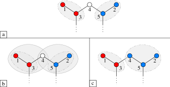
Figure 1: Example of the decentralized partitioning algorithm described in Section III-B. Panel a: starting islands are fundamental layers. Panel b: additional cyber layers are created. Panel c: Letting 4 be a load, it is attached to the blue island, as it has a larger(positive) power balance. The Fundamental layers are then updated.

input : node $j^{*}$, neighbors $\mathcal{N}_{j^{*}}$

output : the microgrid index $l^{*}$ node $j^{*}$ will attach to

$l^{*}\leftarrow\emptyset$;

while $\mathcal{N}_{j^{*}}\cap\left(\bigcup_{l}\mathcal{M}_{l}\right)=\emptyset$ do

       idle;

      

1while $l^{*}=\emptyset$ do

       $\mu_{j^{*}}\leftarrow\{l\mid\exists l:k\in\mathcal{M}_{l},\forall k\in\mathcal{N}_{j^{*}}\}$;

       for $l\in\mu(j^{*})$ do

             if $\Gamma_{l}^{j^{*}}$ does not exist then

                   create $\Gamma_{l}^{j^{*}}$;

                  

            

      Simulate the dynamics on all active layers;

       for $l\in\mu_{j^{*}}$ do

             $t_{l}^{j^{*}}\leftarrow\ \{\bar{t}:|\dot{\theta}_{i}(t)-\dot{\theta}_{j^{*}}(t)|\leq\epsilon\ \forall i\in\mathcal{M}_{l}\cap\mathcal{N}_{j^{*}},\ \forall t\geq\bar{t}\}$;

            

      $t^{j^{*}}\leftarrow\max_{l\in\mu_{j^{*}}}t_{l}^{j^{*}}$;

       for $l\in\mu_{j^{*}}$ do

             $P(l)\leftarrow\bar{\omega}_{l}(\bar{\omega}_{l}^{j^{*}}-P_{j^{*}})/(\bar{\omega}_{l}-\bar{\omega}_{l}^{j^{*}})$;

            

      if  $\exists l:\mathcal{N}_{j^{*}}\subseteq\mathcal{M}_{l}$ then

             $l^{*}\leftarrow l:\mathcal{N}_{j^{*}}\subseteq\mathcal{M}_{l}$

      else

             if $P_{j^{*}}<0$ then

                   if $\max_{i\in\mu_{j^{*}}}P(i)>0$ then

                         $l^{*}\leftarrow\arg\max_{l\in\mu_{j^{*}}}P(l)$;

                         $\tilde{\omega}\leftarrow\bar{\omega}_{l^{*}}$;

                        

                  else

                         do nothing;

                  

            else

                   $l^{*}\leftarrow\arg\min_{l}P(l)$;

                   $\tilde{\omega}\leftarrow\bar{\omega}_{l^{*}}$;

                  

            

      

while $t<t^{j^{*}}$ do

       for $l\in\mu_{j^{*}}$ do

             if $\lvert\bar{\omega}_{l^{*}}(t)-\tilde{\omega}\rvert\geq\epsilon$ then

                   go to 1;

                  

            

      

$\mathcal{M}_{l^{*}}\leftarrow\mathcal{M}_{l^{*}}\cup j^{*}$;

$l^{*}\leftarrow\emptyset$;

Algorithm 2 Decentralized partitioning

IV Numerical Validation

In this section, we validate our partitioning algorithms on the IEEE 118 test case, for which other partitions are available in the literature. To quantitatively assess the performance of our algorithms, we will use the metrics presented in the next section.

IV-A Partition Metrics

We consider the following metrics from [1, 16, 21, 2]:

$$J_{1}\coloneqq\frac{1}{n_{\mu}}\sum^{n_{\mu}}_{l=1}|P(l)|,$$ (15a)

$$J_{2}\coloneqq\frac{1}{n_{\mu}}\sum^{n_{\mu}}_{l=1}\left(1-\frac{V_{\text{min},l}}{V_{\text{max},l}}\right),$$ (15b)

$$J_{3}\coloneqq\sum_{(i,j)\in\mathcal{E}_{l}\ \forall l}|P_{\text{loss},ij}|,$$ (15c)

$$J_{4}\coloneqq\sum_{i\in V_{k},j\in V_{h},k\neq h}\frac{|P_{ij}|+|P_{ji}|}{2}.$$ (15d)

In (15): $P(l)$ is the power imbalance in the $l$-th island and is defined in (10); $V_{\min,l}$ and $V_{\max,l}$ are the minimum and maximum bus voltages among the nodes in the $l$-th island, respectively; $P_{\text{loss},ij}$ is the power loss on line $(i,j)$; finally $P_{ij}$ is the power flowing on line $(i,j)$. Hence,

• $J_{1}$ is the average power imbalance in each island;

• $J_{2}$ is the average voltage deviation in each island and is a measure of the quality of the dispatched power;

• $J_{3}$ is the sum of the power losses in the islands;

• $J_{4}$ is the power disruption induced by the partition, i.e., the sum of the power that was transmitted when the grid was connected on the lines cut to obtain the partition.

We obtain all the quantities required to compute the metrics in (15) by solving for each test case an AC Optimal Power Flow (OPF) using Matpower 6.0 [30]. We leave all the solver options at their default values, except for the cost function, that is chosen to be the total generated power

$$P_{\mathrm{gen}}:=\sum_{i\in\mathcal{V}^{\text{gen}}}P_{i}.$$

Note that all the input parameters required to solve the OPF are available in Matpower for our test case.

IV-B IEEE test case 118

We consider the problem of partitioning the IEEE 118 bus system in $n_{\mu}=2$ islands. We restrict the set of generators $\mathcal{V}^{\text{gen}}$ to be composed only of the 19 synchronous machines present in this test case. Namely, we do not consider the reactive compensators and the synchronous motors, so as to make our partition comparable with that in [16], which we will use as a benchmark. Moreover, we assume that line 14-15 disconnects due to a three phase solid ground fault at bus 15.

To obtain our partitions, we start by applying the procedure outlined in section III. Namely, we initialise the islands to the two sets of coherent synchronous machines which we take from [16]. As the subgraphs of $\mathcal{G}$ defined by this initialisation are not connected, we complement the coherent generators in each set with nodes taken from the shortest paths connecting them, thus obtaining

$$\mathcal{M}_{1} =\{3,5,8,9,10,12,17,25,26,30,31\},$$

$$\mathcal{M}_{2} =\{45,46,49,54,59,61,65,66,69,77,80,82,$$

$$\phantom{={}}83,85,86,87,89,98,100,103,110,111\}$$

as the node sets of the initial connected islands.

Next, we apply Algorithm 1 to obtain a partition in a centralised fashion. The resulting islands, whose power imbalance is $P(1)=-93$ MW and $P(2)=172$ MW, respectively, are shown in Figure 2(a). On the other hand, applying the decentralised Algorithm 2, we obtain the islands in Figure 2. In this case, the power imbalance in each island is $P(1)=-154$ MW and $P(2)=233$ MW.

To evaluate the performance of our algorithms, we compare the values of the metrics (15) evaluated on the partitions we obtained and on the benchmark partition in [16], also shown in Figure 2(c). Let us note that in [16] the authors allow for high voltage DC connections between the islands. As we do not consider DC transmission lines, we compute the metrics (15) for the partition in [16] neglecting their effect. Interestingly, both the partitions obtained from Algorithm 1 and Algorithm 2 perform better than that of ref. [16] in terms of power imbalance $(J_{1})$. On the other hand while we observe worse values of the power disruption $(J_{4})$. All three partitions exhibit instead comparable values in terms of voltage deviations $J_{2}$ and power losses $J_{3}$. Overall, both our partitions present comparable values of the metrics in (15) with respect to that in ref. [16].

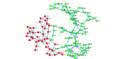
(a)

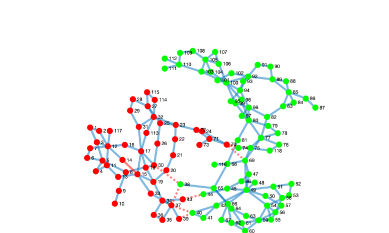
(b)

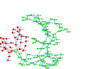
(c)

Figure 2: Three different partitions of the IEEE test case 118 in two islands obtained by applying (a) Algorithm 1, (b) Algorithm 2, and (c) the procedure in [16]. The nodes in red belong to island $1$, while the nodes in green belong to island $2$. Red dashed lines represent the cut-set edges dividing the islands while the failed transmission line is the red solid line.

Metric	[16] (no DC lines)	Centralised	Decentralised
$J_{1}$	$289$	$133$	$194$
$J_{2}$	$0.0835$	$0.0965$	$0.0944$
$J_{3}$	$37.7$	$36.4$	$36.8$
$J_{4}$	$305$	$384$	$509$

TABLE I: values of the metrics computed for the partitions depicted in Figure 2.

Our results suggest that the quality of our partitions, measured according to the established metrics available in the literature, is comparable to that of the partitions obtained by solving a more cumbersome combinatorial optimization problem. FUture work will be aimed at refining our methodology proving its convergence towards a viable partition of a desired grid.

References

- [1] H. Haddadian and R. Noroozian, “Multi-microgrids approach for design and operation of future distribution networks based on novel technical indices,” Applied energy, vol. 185, pp. 650–663, 2017.
- [2] S. A. Arefifar, A.-R. M. Yasser, and T. H. El-Fouly, “Optimum microgrid design for enhancing reliability and supply-security,” IEEE Transactions on Smart Grid, vol. 4, no. 3, pp. 1567–1575, 2013.
- [3] F. Dörfler, J. W. Simpson-Porco, and F. Bullo, “Breaking the hierarchy: Distributed control and economic optimality in microgrids,” IEEE Transactions on Control of Network Systems, vol. 3, no. 3, pp. 241–253, 2015.
- [4] A. Bidram and A. Davoudi, “Hierarchical structure of microgrids control system,” IEEE Transactions on Smart Grid, vol. 3, no. 4, pp. 1963–1976, 2012.
- [5] P. Frasca, H. Ishii, C. Ravazzi, and R. Tempo, “Distributed randomized algorithms for opinion formation, centrality computation and power systems estimation: A tutorial overview,” European journal of control, vol. 24, pp. 2–13, 2015.
- [6] J. Rocabert, A. Luna, F. Blaabjerg, and P. Rodriguez, “Control of power converters in ac microgrids,” IEEE transactions on power electronics, vol. 27, no. 11, pp. 4734–4749, 2012.
- [7] A. Tayyebi, D. Groß, A. Anta, F. Kupzog, and F. Dörfler, “Frequency stability of synchronous machines and grid-forming power converters,” IEEE Journal of Emerging and Selected Topics in Power Electronics, vol. 8, no. 2, pp. 1004–1018, 2020.
- [8] C. Arghir, T. Jouini, and F. Dörfler, “Grid-forming control for power converters based on matching of synchronous machines,” Automatica, vol. 95, pp. 273–282, 2018.
- [9] F. Milano, F. Dörfler, G. Hug, D. J. Hill, and G. Verbič, “Foundations and challenges of low-inertia systems,” in 2018 Power Systems Computation Conference (PSCC). IEEE, 2018, pp. 1–25.
- [10] F. Dörfler, S. Bolognani, J. W. Simpson-Porco, and S. Grammatico, “Distributed control and optimization for autonomous power grids,” in 2019 18th European Control Conference (ECC). IEEE, 2019, pp. 2436–2453.
- [11] G. Lalor, A. Mullane, and M. O’Malley, “Frequency control and wind turbine technologies,” IEEE Transactions on power systems, vol. 20, no. 4, pp. 1905–1913, 2005.
- [12] H. Bevrani, A. Ghosh, and G. Ledwich, “Renewable energy sources and frequency regulation: survey and new perspectives,” IET Renewable Power Generation, vol. 4, no. 5, pp. 438–457, 2010.
- [13] A. Ulbig, T. S. Borsche, and G. Andersson, “Impact of low rotational inertia on power system stability and operation,” IFAC Proceedings Volumes, vol. 47, no. 3, pp. 7290–7297, 2014.
- [14] Z. Wang, B. Chen, J. Wang, M. M. Begovic, and C. Chen, “Coordinated energy management of networked microgrids in distribution systems,” IEEE Transactions on Smart Grid, vol. 6, no. 1, pp. 45–53, 2014.
- [15] N. Nikmehr and S. N. Ravadanegh, “Optimal power dispatch of multi-microgrids at future smart distribution grids,” IEEE transactions on smart grid, vol. 6, no. 4, pp. 1648–1657, 2015.
- [16] X. Fan, E. Crisostomi, D. Thomopulos, B. Zhang, and S. Yang, “A controlled islanding algorithm for ac/dc hybrid power systems utilizing dc modulation,” IET Generation, Transmission & Distribution, accepted for publication, 2021.
- [17] S. Pahwa, M. Youssef, P. Schumm, C. Scoglio, and N. Schulz, “Optimal intentional islanding to enhance the robustness of power grid networks,” Physica A: Statistical Mechanics and its Applications, vol. 392, no. 17, pp. 3741–3754, 2013.
- [18] K. Sun, D.-Z. Zheng, and Q. Lu, “Splitting strategies for islanding operation of large-scale power systems using obdd-based methods,” IEEE transactions on Power Systems, vol. 18, no. 2, pp. 912–923, 2003.
- [19] M. Adibi, R. Kafka, S. Maram, and L. M. Mili, “On power system controlled separation,” IEEE Transactions on Power Systems, vol. 21, no. 4, pp. 1894–1902, 2006.
- [20] P. Fernández-Porras, M. Panteli, and J. Quirós-Tortós, “Intentional controlled islanding: when to island for power system blackout prevention,” IET Generation, Transmission & Distribution, vol. 12, no. 14, pp. 3542–3549, 2018.
- [21] S. A. Arefifar, Y. A.-R. I. Mohamed, and T. H. El-Fouly, “Supply-adequacy-based optimal construction of microgrids in smart distribution systems,” IEEE transactions on smart grid, vol. 3, no. 3, pp. 1491–1502, 2012.
- [22] S. A. Arefifar and Y. A.-R. I. Mohamed, “Dg mix, reactive sources and energy storage units for optimizing microgrid reliability and supply security,” IEEE Transactions on Smart Grid, vol. 5, no. 4, pp. 1835–1844, 2014.
- [23] F. Moghateli, S. A. Taher, A. Karimi, and M. Shahidehpour, “Multi-objective design method for construction of multi-microgrid systems in active distribution networks,” IET Smart Grid, vol. 3, no. 3, pp. 331–341, 2020.
- [24] S. Hasanvand, M. Nayeripour, E. Waffenschmidt, and H. Fallahzadeh-Abarghouei, “A new approach to transform an existing distribution network into a set of micro-grids for enhancing reliability and sustainability,” Applied Soft Computing, vol. 52, pp. 120–134, 2017.
- [25] S. Mohammadi, S. Soleymani, and B. Mozafari, “Scenario-based stochastic operation management of microgrid including wind, photovoltaic, micro-turbine, fuel cell and energy storage devices,” International Journal of Electrical Power & Energy Systems, vol. 54, pp. 525–535, 2014.
- [26] S. Sastry and P. Varaiya, “Coherency for interconnected power systems,” IEEE Transactions on Automatic Control, vol. 26, no. 1, pp. 218–226, 1981.
- [27] Z. Lin, F. Wen, Y. Ding, Y. Xue, S. Liu, Y. Zhao, and S. Yi, “Wams-based coherency detection for situational awareness in power systems with renewables,” IEEE Transactions on Power Systems, vol. 33, no. 5, pp. 5410–5426, 2018.
- [28] J. Wei and D. Kundur, “A multi-flock approach to rapid dynamic generator coherency identification,” in 2013 IEEE Power & Energy Society General Meeting. IEEE, 2013, pp. 1–5.
- [29] F. Dörfler and F. Bullo, “Synchronization in complex networks of phase oscillators: A survey,” Automatica, vol. 50, no. 6, pp. 1539–1564, 2014.
- [30] R. D. Zimmerman, C. E. Murillo-Sánchez, and R. J. Thomas, “Matpower: Steady-state operations, planning, and analysis tools for power systems research and education,” IEEE Transactions on power systems, vol. 26, no. 1, pp. 12–19, 2010.