Mimetic Tensor-Vector-Scalar Cosmology:
Incorporating Dark Matter, Dark Energy and Stiff Matter

Abstract

Phenomenological implications of the Mimetic Tensor-Vector-Scalar theory (MiTeVeS) are studied. The theory is an extension of the vector field model of mimetic dark matter, where a scalar field is also incorporated, and it is known to be free from ghost instability. In the absence of interactions between the scalar field and the vector field, the obtained cosmological solution corresponds to the General theory of Relativity (GR) with a minimally-coupled scalar field. However, including an interaction term between the scalar field and the vector field yields interesting dynamics. There is a shift symmetry for the scalar field with a flat potential, and the conserved Noether current, which is associated with the symmetry, behaves as a dark matter component. Consequently, the solution contains a cosmological constant, dark matter and a stiff matter fluid. Breaking the shift symmetry with a non-flat potential gives a natural interaction between dark energy and dark matter.

Keywords: tensor-vector-scalar gravity, mimetic dark matter, dark energy, stiff matter, cosmological constraints

I Introduction

The Universe is found from many experiments and observations to include 25% of matter and 68% of dark energy Riess et al. (1998); Perlmutter et al. (1999); Abbott et al. (2018); Aghanim et al. (2020). There have been many models for dark matter Bertone et al. (2005); Roszkowski et al. (2018); Arkani-Hamed et al. (2009); Cyr-Racine and Sigurdson (2013); Foot and Vagnozzi (2015). The description of dark energy, however, suffers from theoretical problems Weinberg (1989); Sahni (2002); Copeland et al. (2006); Cai et al. (2010)), what gives motivation for modified theories of gravity Tsujikawa (2010); Capozziello and De Laurentis (2011); Nojiri et al. (2017), as the General Relativity (GR) could not describe the data through the whole range of scales. One interesting class of modified theories of gravity are theories, where a scalar field mimics the dark matter Chamseddine and Mukhanov (2013) using a Lagrange multiplier Golovnev (2014); Chamseddine et al. (2014) (see also Sebastiani et al. (2017) for a review and Arroja et al. (2015, 2016); Ganz et al. (2019); Casalino et al. (2018) for some developments of the mimetic theory). In its original formulation, the mimetic theory of gravity can be obtained starting from the GR with a Lagrange multiplier that forces the kinetic part of the scalar field to behave as a constant in time Barvinsky (2014). Consequently, the contribution of the mimetic field in the gravitational field equations is a pressureless perfect fluid. On a Friedmann-Robertson-Walker (FRWM) metric this fluid behaves precisely as a dust component on the cosmological scales. A minimal generalization of the mimetic dark matter was proposed by including a potential for the mimetic scalar field Chamseddine et al. (2014). The cosmological dynamics of the theory was further studied in Dutta et al. (2018). The theory contains dynamic dark energy along with mimetic dark matter, and it was stressed that the early-time solution is not dominated by stiff matter unlike in simpler scalar-field models of dark energy, like in quintessence.

The Modified Newtonian Dynamics (MOND) Milgrom (1983); Bekenstein and Milgrom (1984) is also an alternative successful explanation for the flat rotation curves of galaxies. By violating the Newton’s second law at low accelerations, the Tully-Fisher relation is recovered, without introducing an additional dark matter  Tully and Fisher (1977); McGaugh et al. (2000); Chae et al. (2020). The Tensor-Vector-Scalar theory (TeVeS) is a covariant theory, which produces MOND in the low energy limit Bekenstein (2004). TeVeS is a stable theory and free from ghosts  Chaichian et al. (2014a). A new relativistic theory for MOND has been proposed Skordis and Zlosnik (2021) in order to reproduce the key cosmological observations, while still reproducing all the galactic and lensing phenomenology in the same way as TeVeS does.

Cosmology with vector fields has been considered widely in the literature Kase and Tsujikawa (2018); Heisenberg et al. (2019); Oliveros and Jaraba (2019); Gallego Cadavid and Rodriguez (2019); Kushwaha and Shankaranarayanan (2020); Benisty and Guendelman (2018). General consideration of scalar-vector-tensor theories and their cosmological solutions is given in Heisenberg et al. (2018). A vector field model of mimetic matter was proposed in Barvinsky (2014). The consistency of those theories with respect to the absence of ghost instability was studied in Chaichian et al. (2014b), including a proposal of a new Tensor-Vector-Scalar gravity (MiTeVeS), which generalizes the previous models. The vector field was introduced to enable the possibility of rotating flows of mimetic matter and to avoid caustics of the geodesic flow Barvinsky (2014). The scalar field in MiTeVeS, with its coupling to the vector field, has a significant impact on cosmology. In this paper we discover the homogeneous solution for this theory considering couple of possible interactions for the vector and scalar fields.

First in section III we confirm that the theory with the added interactions does not suffer from pathologies like ghosts, gradient instabilities or tachyons. The homogeneous solution is obtained in sections IV and V. Cosmological constraints on the solution are obtained in section VI. Interacting dark energy and dark matter are discussed in section VII.

II The Theory

II.1 Lagrangian

Gravitational theories with mimetic matter involve two metrics which are related by a conformal transformation. The physical metric $\Phi^{2}g_{\mu\nu}$ is coupled minimally to all matter fields, where $\Phi$ is the conformal factor field that relates the physical metric to the metric $g_{\mu\nu}$. The Mimetic TeVeS theory includes a scalar field $\phi$ and a vector field $u_{\mu}$. The conformal factor is related to the scalar and vector fields by including a constraint with a Lagrange multiplier $\lambda$. The Lagrangian is written as

$$\begin{split}\mathcal{L}=\frac{1}{2}\Phi^{2}\mathcal{R}+3\Phi^{,\alpha}\Phi_{,\alpha}-\frac{1}{2}\lambda\left(\Phi^{2}+f(\phi)\,u^{\mu}u_{\mu}\right)\\ -\frac{\Phi^{2}}{2}\phi_{,\mu}\phi^{,\mu}-\Phi^{4}V(\phi)-\frac{\mu^{2}}{4}F_{\mu\nu}F^{\mu\nu}+\mathcal{L}_{\mathrm{m,int}},\end{split}$$ (1)

where $\mathcal{R}$ is the Ricci scalar determined by the metric $g_{\mu\nu}$, the kinetic term of the vector field is defined in terms of

$$F_{\mu\nu}=\partial_{\mu}u_{\nu}-\partial_{\nu}u_{\mu},$$ (2)

and the Lagrangian density $\mathcal{L}_{\mathrm{m,int}}(\Phi^{2}g_{\mu\nu},\chi,\partial\chi,u_{\mu},\phi,\phi_{,\mu})$ represents matter fields (denoted collectively as $\chi$) and all interactions among the gravitational fields and the matter fields. Matter couples universally to the physical metric $\Phi^{2}g_{\mu\nu}$.

The concept of scale invariance is an attractive possibility for a fundamental symmetry of nature. Dimensionless coupling constants for example appear to be related to good renormalizability properties. In its most naive realizations, scale invariance is not a viable symmetry, since nature seems to have chosen some typical scales. The scale invariance can nevertheless be incorporated into realistic generally covariant field theories. Scale invariance has to be discussed in a more general framework than that of standard generally relativistic theories. In the MiTeVeS theory, the action incorporates the scale invariance under the transformation

$$g_{\mu\nu}\rightarrow L^{2}g_{\mu\nu},\quad\Phi\rightarrow L^{-1}\Phi,\quad\lambda\rightarrow L^{-2}\lambda,$$ (3)

where $L=L(\vec{x},t)$ is an arbitrary function of space and time. The fields $\phi$ and $u_{\mu}$ are the invariant of the theory:

$$\phi\rightarrow\phi,\quad u_{\mu}\rightarrow u_{\mu}.$$ (4)

This indicates that the theory is capable to have inflationary solutions naturally.

We can simplify the derivation of the field equations by fixing the conformal symmetry of the theory. We shall choose the gauge condition as $\Phi=1$, which gives the theory in the Einstein frame form Chaichian et al. (2014b). This is equivalent to performing the following conformal transformation in (1):

$$g_{\mu\nu}\rightarrow\Phi^{-2}g_{\mu\nu},\quad\lambda\rightarrow\Phi^{2}\lambda.$$ (5)

In this frame the Lagrangian is obtained without the auxiliary field $\Phi$ as

$$\begin{split}\mathcal{L}=\frac{1}{2}\mathcal{R}(g_{\mu\nu})-\frac{1}{2}\lambda\left(1+f(\phi)\,u^{\mu}u_{\mu}\right)-\frac{1}{2}\phi_{,\mu}\phi^{,\mu}\\ -V(\phi)-\frac{\mu^{2}}{4}F_{\mu\nu}F^{\mu\nu}+\mathcal{L}_{\mathrm{m,int}},\end{split}$$ (6)

where $g_{\mu\nu}$ is now the physical metric that couples to matter universally. This frame is equivalent for the setting

$$\Phi^{2}=\frac{1}{8\pi G}=1$$ (7)

where $G$ is the Newtonian Constant. We assume in the following analyses that the gravitational vector and scalar fields do not couple directly to matter fields:

$$\mathcal{L}_{\mathrm{m,int}}=\mathcal{L}_{\mathrm{m}}(g_{\mu\nu},\chi,\partial\chi)+\mathcal{L}_{\mathrm{int}}(g_{\mu\nu},u_{\mu},\phi,\phi_{,\mu}).$$ (8)

Furthermore, we consider the two simplest interactions for $\phi$ and $u_{\mu}$,

$$\mathcal{L}_{\mathrm{int}}=-\frac{1}{2}h_{1}(\phi)u_{\mu}u^{\mu}-\frac{1}{2}h_{2}(\phi)u^{\mu}\phi_{,\mu},$$ (9)

which involve $u_{\mu}$ up to the second power and are at most linear in $\phi_{,\mu}$. Terms that involve higher powers of $\phi_{,\mu}$ would modify the kinetic term of the scalar field $\phi$, which will not be considered in this work. These assumptions on $\mathcal{L}_{\mathrm{m,int}}$ are made here mainly for simplicity. More generally, interactions of higher order as well as couplings between matter and the scalar and/or vector fields are possible. We also note that quantum corrections may induce such terms, when there is no symmetry to prevent it.

II.2 Field equations

Varying the Lagrangian (6) minimally coupled to the interaction term (9) with respect to $g^{\mu\nu}$, $\lambda$, $\phi$ and $u_{\mu}$ gives the field equations as

$$G_{\mu\nu}=\lambda f(\phi)u_{\mu}u_{\nu}+T^{\phi}_{\mu\nu}+T^{u}_{\mu\nu}+T_{\mu\nu}^{\mathrm{int},1}+T_{\mu\nu}^{\mathrm{int},2}+T_{\mu\nu},$$ (10a)

$$f(\phi)\,u^{\mu}u_{\mu}=-1,$$ (10b)

$$\Box\phi+\frac{1}{2}h_{2}(\phi)\nabla_{\mu}u^{\mu}=V^{\prime}(\phi)+\frac{1}{2}\left(\lambda f^{\prime}(\phi)+h_{1}^{\prime}(\phi)\right)u^{\mu}u_{\mu},$$ (10c)

$$\mu^{2}\nabla_{\nu}F^{\nu\mu}=\left[\lambda f(\phi)+h_{1}(\phi)\right]u^{\mu}+\frac{1}{2}h_{2}(\phi)\phi^{,\mu},$$ (10d)

where in the modified Einstein equation (10a) we have defined the energy-momentum tensors as:

$$T^{\phi}_{\mu\nu}=\phi_{,\mu}\phi_{,\nu}-g_{\mu\nu}\left(\frac{1}{2}\phi_{,\alpha}\phi^{,\alpha}+V(\phi)\right),$$ (11)

$$T^{u}_{\mu\nu}=\mu^{2}\left(F_{\mu\rho}F_{\nu}^{\phantom{\nu}\rho}-\frac{1}{4}g_{\mu\nu}F_{\rho\sigma}F^{\rho\sigma}\right),$$ (12)

$$T_{\mu\nu}=-\frac{2}{\sqrt{-g}}\frac{\delta}{\delta g^{\mu\nu}}\int d^{4}x\sqrt{-g}\,\mathcal{L}_{\mathrm{m}}(g_{\mu\nu},\chi,\partial\chi),$$ (13)

$$T_{\mu\nu}^{\mathrm{int},1}=h_{1}(\phi)\left(u_{\mu}u_{\nu}-\frac{1}{2}g_{\mu\nu}\left(u^{\alpha}u_{\alpha}\right)\right),$$ (14)

$$T_{\mu\nu}^{\mathrm{int},2}=h_{2}(\phi)\left(u_{(\mu}\phi_{,\nu)}-\frac{1}{2}g_{\mu\nu}\left(u^{\alpha}\phi_{,\alpha}\right)\right),$$ (15)

where the parentheses around indices denote symmetrization:

$$u_{(\mu}\phi_{,\nu)}=\frac{1}{2}\left(u_{\mu}\phi_{,\nu}+u_{\nu}\phi_{,\mu}\right),$$ (16)

which ensures the symmetric form of the energy momentum tensor. The contributions of the interactions between the scalar field and the vector field to the energy-momentum tensor are given in (14) and (15).

III Healthiness of the theory

In this section we discuss the absence of ghosts, propagation of perturbations and stability, particularly regarding the interactions that we have introduced in (9). First we complete the Hamiltonian analysis Chaichian et al. (2014b) with the interactions (9). The structure of the Hamiltonian analysis remains largely unchanged, since the interactions (9) involve only one derivative of the scalar field. Hence we only present the significant changes to the Hamiltonian analysis achieved in Chaichian et al. (2014b). We have performed the Hamiltonian analysis of MiTeVeS with the usual method suited for constrained systems Gitman and Tyutin (1990); Henneaux and Teitelboim (1992); Chaichian and Demichev (2001).

In the last subsection we discuss the relation of MiTeVeS and the Einstein-aether theory of gravity, particularly regarding the requirements of stability.

III.1 Hamiltonian analysis

We assume foliation of spacetime to a union of spacelike hypersurfaces and the Arnowitt–Deser–Misner parameterization of the metric,

$$ds^{2}=-N^{2}dt^{2}+h_{ij}(N^{i}dt+dx^{i})(N^{j}dt+dx^{j}).$$

The variables of the Hamiltonian formulation are the lapse $N$, the shift $N^{i}$, the induced metric $h_{ij}$ on the spatial hypersurface, the scalar fields $\lambda$, $\Phi$ and $\phi$, and the components of the vector field $u_{i}$ and $u_{\mathbf{n}}$ that are tangent and normal to the spatial hypersurfaces, respectively. The canonical momenta conjugate to those variables are $\pi_{N}$, $\pi_{i}$, $\pi^{ij}$, $p_{\lambda}$, $p_{\Phi}$, $p_{\phi}$, $p^{i}$ and $p_{\mathbf{n}}$, respectively. The covariant derivative determined by the metric $h_{ij}$ is denoted with $D$, and $R$ is the corresponding Ricci scalar.

We obtain the Hamiltonian as

$$H=\int d^{3}x\,\Bigl{(}N\mathcal{H}_{T}+N^{i}\mathcal{H}_{i}+v_{\mathcal{D}}\mathcal{D}+v_{N}\pi_{N}+v^{i}\pi_{i}\\ +v_{\lambda}p_{\lambda}+v_{\mathbf{n}}p_{\mathbf{n}}\Bigr{)},$$ (17)

where

$$\mathcal{H}_{T} =\frac{2}{\sqrt{h}\Phi^{2}}\pi^{ij}\mathcal{G}_{ijkl}\pi^{kl}-\frac{1}{2}\sqrt{h}R\Phi^{2}+\partial_{i}[\sqrt{h}h^{ij}\partial_{j}\Phi^{2}]$$

$$-3\sqrt{h}h^{ij}\partial_{i}\Phi\partial_{j}\Phi-\frac{1}{2}\sqrt{h}\lambda\bigl{(}\Phi^{2}+f(\phi)u_{i}h^{ij}u_{j}$$

$$-f(\phi)u_{\mathbf{n}}^{2}\bigr{)}+\frac{1}{2\mu^{2}\sqrt{h}}p^{i}h_{ij}p^{j}$$

$$+\frac{\mu^{2}}{4}\sqrt{h}h^{ik}h^{jl}(D_{i}u_{j}-D_{j}u_{i})(D_{k}u_{l}-D_{l}u_{k})$$

$$-u_{\mathbf{n}}D_{i}p^{i}+\frac{1}{2}\sqrt{h}\Phi^{2}h_{1}(\phi)\left(u_{i}h^{ij}u_{j}-u_{\mathbf{n}}^{2}\right)$$

$$+\frac{1}{8}\sqrt{h}\Phi^{2}\left(h_{2}(\phi)u_{\mathbf{n}}\right)^{2}+\frac{p_{\phi}^{2}}{2\sqrt{h}\Phi^{2}}-\frac{1}{2}h_{2}(\phi)u_{\mathbf{n}}p_{\phi}$$

$$+\frac{1}{2}\sqrt{h}\Phi^{2}\partial_{i}\phi\,h^{ij}\left(\partial_{j}\phi+h_{2}(\phi)u_{j}\right)+\sqrt{h}\Phi^{4}V(\phi),$$ (18)

$$\mathcal{H}_{i} =p_{\Phi}\partial_{i}\Phi-2h_{ik}D_{j}\pi^{kj}+\partial_{i}u_{j}p^{j}-\partial_{j}(u_{i}p^{j})+p_{\phi}\partial_{i}\phi,$$ (19)

$$\mathcal{D} =p_{\Phi}\Phi-2\pi^{ij}h_{ij}.$$ (20)

In (17) all the fields denoted with $v$ are Lagrange multipliers. We have denoted the De Witt metric in (18) as

$$\mathcal{G}_{ijkl}=\frac{1}{2}(h_{ik}h_{jl}+h_{il}h_{jk})-\frac{1}{2}h_{ij}h_{kl}.$$

The primary constraints are

$$p_{\lambda} \approx 0,\quad\pi_{N}\approx 0,\quad\pi_{i}\approx 0,\quad p_{\mathbf{n}}\approx 0,$$

$$\tilde{\mathcal{D}} =p_{\Phi}\Phi-2\pi^{ij}h_{ij}+2p_{\lambda}\lambda+p_{\mathbf{n}}u_{\mathbf{n}}\approx 0.$$ (21)

The preservation of the primary constraints $\pi_{N}$ and $\pi^{i}$ during the time evolution of the system implies following secondary constraints

$$\mathcal{H}_{T}\approx 0,\quad\mathcal{H}_{i}\approx 0.$$ (22)

The requirement of the preservation of the constraint $p_{\lambda}\approx 0$ implies a secondary constraint,

$$\mathcal{C}_{\lambda}=\sqrt{h}\left(\Phi^{2}+f(\phi)u_{i}h^{ij}u_{j}-f(\phi)u_{\mathbf{n}}^{2}\right)\approx 0.$$ (23)

The preservation of the constraint $p_{\mathbf{n}}$ gives a secondary constraint,

$$\mathcal{C}_{\mathbf{n}}=\sqrt{h}\left(\Phi^{2}h_{1}(\phi)-\lambda f(\phi)-\frac{1}{4}\Phi^{2}h_{2}^{2}(\phi)\right)u_{\mathbf{n}}\\ +D_{i}p^{i}+\frac{1}{2}h_{2}(\phi)p_{\phi}\approx 0.$$ (24)

The constraint $\tilde{\mathcal{D}}$ is the first class constraint that generates the scaling transformation. $\mathcal{H}_{T}$, $\pi_{N}$, $\mathcal{H}_{i}$ and $\pi_{i}$ are the first class constraints which reflect of the diffeomorphism invariance of the theory. The four remaining constraints $p_{\lambda}$, $\mathcal{C}_{\mathbf{n}}$, $p_{\mathbf{n}}$ and $\mathcal{C}_{\lambda}$ are the second class constraints, which can be interpreted as follows. The constraints $p_{\lambda}$ and $\mathcal{C}_{\mathbf{n}}$ can be used to fix the pair of canonical variables $\lambda$ and $p_{\lambda}$, while the constraints $p_{\mathbf{n}}$ and $\mathcal{C}_{\lambda}$ can be used to fix the variables $u_{\mathbf{n}}$ and $p_{\mathbf{n}}$. Overall the Hamiltonian structure remains similar to Chaichian et al. (2014b).

There is no sign of presence of ghosts in the Hamiltonian.

III.2 Propagation of perturbations

We consider the linearization of the theory. The tensor, vector and scalar fields are written as

$$g_{\mu\nu}=g^{(0)}_{\mu\nu}+\bar{g}_{\mu\nu},\quad u_{\mu}=u^{(0)}_{\mu}+\bar{u}_{\mu},\quad\phi=\phi^{(0)}+\bar{\phi},$$ (25)

where $g^{(0)}_{\mu\nu}$, $u^{(0)}_{\mu}$ and $\phi^{(0)}$ are the background and $\bar{g}_{\mu\nu}$, $\bar{u}_{\mu}$ and $\bar{\phi}$ are small amplitude perturbations with a length scale of variations much shorter than the length scale of variation of the background. We study the propagation of perturbations

For simplicity we consider the Minkowski background: $g^{(0)}_{\mu\nu}=\eta_{\mu\nu}$, $\phi^{(0)}=\phi_{0}$ (constant) and $u^{(0)}_{\mu}=(f(\phi_{0})^{-\frac{1}{2}},0,0,0)$. This background can be obtained in the limit of vanishing mimetic energy-momentum in the background: $V(\phi_{0})=-\lambda/2$ and $h_{1}(\phi_{0})=-\lambda f(\phi_{0})$.

We consider the field equations (10d) to lowest order in the perturbations. The Einstein field equations (10a) are linearized as $\bar{G}_{\mu\nu}=T^{tot}_{\mu\nu}$, where $\bar{G}_{\mu\nu}$ is the linearized Einstein tensor and $T^{tot}_{\mu\nu}$ is the total energy-momentum, where the scalar and vector fields appear like additional matter components. The propagation of the metric perturbations is similar to GR. The rest of the field equations give the linearized constraint

$$-\frac{f^{\prime}(\phi_{0})}{f(\phi_{0})}\bar{\phi}+\bar{g}^{00}-2f(\phi_{0})^{\frac{1}{2}}\bar{u}_{0}=0,$$ (26)

and the linearized field equations for the scalar and vector fields

$$\Box\bar{\phi}+\frac{1}{2}h_{2}\partial_{\mu}\bar{u}^{\mu} =B\bar{\phi},$$ (27a)

$$\mu^{2}\left(\Box\bar{u}^{\mu}-\partial^{\mu}\partial_{\nu}\bar{u}^{\nu}\right) =\frac{1}{2}h_{2}(\phi_{0})\bar{\phi}^{,\mu},$$ (27b)

where we have defined

$$B=V^{\prime\prime}(\phi_{0})-\left(\frac{\lambda f^{\prime}+h_{1}^{\prime}}{2f}\right)^{\prime}(\phi_{0}).$$ (28)

For the constant functions (52) considered in Sec. V we would have $B=0$. The constraint (26) determines one of the three involved perturbations in terms of the other two. Differentiating the vector equation (27b) we obtain $\Box\bar{\phi}=0$, which according to the scalar equation (27a) implies $h_{2}(\phi_{0})\partial_{\mu}\bar{u}^{\mu}=2B\bar{\phi}$; in the case of the constant functions (52) the perturbation of the vector field is transverse. Hence the scalar and vector equations (27) simplify as

$$\Box\bar{\phi} =0,$$ (29a)

$$\Box\bar{u}_{\mu} =\frac{C}{\mu^{2}}\bar{\phi}_{,\mu},$$ (29b)

where we have defined

$$C=\frac{1}{2}h_{2}(\phi_{0})+\frac{2\mu^{2}B}{h_{2}(\phi_{0})}.$$ (30)

The functions $V$, $f$, $h_{1}$ and $h_{2}$ are chosen so that $C\geq 0$.

The perturbations of the tensor and scalar fields satisfy standard wave equations and propagate with the speed of light ($c=1$). The perturbation $\bar{u}_{\mu}$ of the vector field satisfies the forced wave equation (29b), where the forcing term is the gradient of the scalar perturbation. The solution of (29b) is a sum of the solution of the homogeneous wave equation $\Box\bar{u}_{\mu}=0$ and the solution of the inhomogeneous wave equation, $\bar{u}_{\mu}=\bar{u}_{\mu}^{H}+\bar{u}_{\mu}^{I}$. The latter can be written with a Green’s function as

$$\bar{u}_{\mu}^{I}=\frac{C}{\mu^{2}}\int d^{4}y\,G(x-y)\bar{\phi}_{,\mu}(y),$$ (31)

where the Green’s function $G$ satisfies $\Box G(x)=\delta(x)$ with suitable boundary conditions. Consider the plane wave solutions to the homogeneous wave equations $\bar{\phi}=\epsilon e^{ik_{\mu}x^{\mu}}$ and $\bar{u}_{\mu}^{H}=\epsilon_{\mu}e^{ik_{\mu}x^{\mu}}$. Then the solution of (29b) takes the form

$$\begin{split}\bar{u}_{\mu}&=\epsilon_{\mu}e^{ik_{\mu}x^{\mu}}+i\epsilon k_{\mu}\frac{C}{\mu^{2}}\int d^{4}y\,G(x-y)e^{ik_{\mu}y^{\mu}}\\ &=\left(\epsilon_{\mu}+i\epsilon\frac{C}{\mu^{2}}\frac{k_{\mu}}{k^{2}+i\varepsilon}\right)e^{ik_{\mu}x^{\mu}},\end{split}$$ (32)

where we have used that the Fourier transformation $\hat{G}(k)$ of the Green’s function satisfies $k^{2}\hat{G}(k)=-1$. This solution tells us three significant things. The solution (32) is a plane wave with a $k$-dependent amplitude and it gives the dispersion relation $k^{2}=0$ by substitution into (29b). The $k$-dependent part of the amplitude of (32) is parallel to $k_{\mu}=(\omega,\mathbf{k})$, which means that if we write $\bar{u}_{\mu}=(\bar{u}_{0},\bm{\bar{u}}^{\perp}+\bm{\bar{u}}^{\parallel})$, where $\bm{\bar{u}}^{\perp}$ is perpendicular to $\mathbf{k}$ and $\bm{\bar{u}}^{\parallel}$ is parallel to $\mathbf{k}$, the perpendicular component $\bm{\bar{u}}^{\perp}=\bm{\epsilon}^{\perp}e^{ik_{\mu}x^{\mu}}$, i.e., only the components $\bar{u}_{0}$ and $\bm{\bar{u}}^{\parallel}$ have $k$-dependent amplitudes. Thirdly, the scale of variation of the amplitude is given by the parameter $C/\mu^{2}$.

The analysis of perturbations on a general curved background is somewhat longer. The key point to observe about the field equations (10d) is that the kinetic matrix of the Lagrangian is diagonal with respect to the tensor, vector and scalar fields, and furthermore it is a direct sum of the Einstein, Klein-Gordon and Maxwell kinetic terms, respectively. Therefore, as long as the functions $V$, $f$, $h_{1}$ and $h_{2}$ are chosen reasonably (as demonstrated above), there are no instabilities or tachyons.

Finally, we remark that the interaction terms we have introduced in (9) represent attractive interactions between the vector and scalar fields. In the linearized theory, the interaction terms $-\frac{1}{2}h_{1}\bar{u}_{\mu}\bar{g}^{\mu\nu}\bar{u}_{\nu}-\frac{1}{2}h_{2}\bar{u}_{\mu}\bar{g}^{\mu\nu}\bar{\phi}_{,\nu}$ describe an interaction of the vector field with itself and an interaction between the vector and scalar fields. Both interactions are mediated by the tensor field, i.e., the graviton, which is a massless spin-2 field. It is well known that an interaction mediated by an even integer spin field is always attractive. Such an attractive interaction cannot drive the system to an illimitably excited state. So it is clear that the addition of these interactions could not have introduced instabilities.

III.3 Relation to Einstein-aether theory and potential issues with stability

When the function $f(\phi)$ is a constant, the vector field $u_{\mu}$ is similar to the aether vector field of Einstein-aether theory Jacobson and Mattingly (2001). In Einstein-aether theory the vector field is constrained to be a timelike unit vector, $u_{\mu}u^{\mu}=-1$. Einstein-aether theory has been studied extensively as a way to consider the consequences of dynamical breaking of local Lorentz invariance such as variation of the speed of light or high frequency dispersion. In our theory, the vector field is coupled to the scalar field $\phi$ in the Lagrangian (6). In this work we only consider the two interactions in (9) in addition to the constaint (10b).

The stability of the aether vector field on Minkowski background spacetime was studied in Carroll et al. (2009). It was found that only three kinetic terms have no linear instabilities or negative-energy ghosts: the sigma model $\partial_{\mu}u_{\nu}\partial^{\mu}u^{\nu}$, the Maxwell term $F_{\mu\nu}F^{\mu\nu}$, and the scalar kinetic term $(\partial_{\mu}u^{\mu})^{2}$. Only for the the sigma model the Hamiltonian of the vector field on the Minkowski background is bounded from below.

The Hamiltonian density of a field on a fixed background should not be confused with the Hamiltonian density of the full gravitational theory. The latter is a sum of constraints, as can be seen in the present case in (17), and thus it is always zero. The total energy of the system can be determined in terms of the boundary terms of the Hamiltonian (similarly as for General Relativity Hawking and Horowitz (1996)). Positivity of the total energy for Einstein-aether theory was shown in Garfinkle and Jacobson (2011) for a class of solutions where the vector field is orthogonal to the spatial hypersurfaces of constant time and has a vanishing divergence on such hypersurfaces. We do not consider the boundedness of the total energy in this work.

Instead, similar to the analysis of Carroll et al. (2009), we consider boundedness of the Hamiltonian of the vector field and the scalar field on the Minkowski background. In other words we fix the metric and ignore its dynamics. Then the Hamiltonian $H=\int d^{3}x\mathcal{H}$ is obtained as

$$\begin{split}\mathcal{H}&=\frac{1}{2\mu^{2}}p^{i}p^{i}+\frac{1}{2}p_{\phi}^{2}-u_{\mathbf{n}}\partial_{i}p^{i}-\frac{1}{2}h_{2}(\phi)u_{\mathbf{n}}p_{\phi}\\ &+\frac{\mu^{2}}{4}(\partial_{i}u_{j}-\partial_{j}u_{i})(\partial_{i}u_{j}-\partial_{j}u_{i})\\ &+\frac{1}{8}\left(h_{2}(\phi)u_{\mathbf{n}}\right)^{2}+\frac{1}{2}\partial_{i}\phi\left(\partial_{i}\phi+h_{2}(\phi)u_{i}\right)+\tilde{V}(\phi).\end{split}$$ (33)

where we have also gauge fixed the conformal symmetry with $\Phi=1$, used the second class constraints, and redefinied the potential of the scalar field as $\tilde{V}(\phi)=V(\phi)+\frac{h_{1}(\phi)}{2f(\phi)}$. Completing the squares in the Hasimilarly miltonian density gives

$$\begin{split}\mathcal{H}&=\frac{1}{2\mu^{2}}\left(p^{i}+\mu^{2}\partial_{i}u_{\mathbf{n}}\right)^{2}-\frac{\mu^{2}}{2}\left(\partial_{i}u_{\mathbf{n}}\right)^{2}\\ &+\frac{\mu^{2}}{4}\left(\partial_{i}u_{j}-\partial_{j}u_{i}\right)^{2}+\frac{1}{2}\left(p_{\phi}-\frac{1}{2}h_{2}(\phi)u_{\mathbf{n}}\right)^{2}\\ &+\frac{1}{2}\left(\partial_{i}\phi+\frac{1}{2}h_{2}(\phi)u_{i}\right)^{2}-\frac{1}{8}\left(h_{2}(\phi)u_{i}\right)^{2}\\ &+\tilde{V}(\phi).\end{split}$$ (34)

Note that $u_{\mathbf{n}}$ is fixed by the constraint (23) as

$$u_{\mathbf{n}}^{2}=\frac{1}{f(\phi)}+u_{i}u_{i}$$ (35)

and the definitions of the canonical momenta are now

$$p^{i}=\mu^{2}\left(\partial_{t}u_{i}-\partial_{i}u_{\mathbf{n}}\right),\quad p_{\phi}=\partial_{t}\phi.$$ (36)

There are two negative terms in the Hamiltonian (34), namely, $-\frac{\mu^{2}}{2}\left(\partial_{i}u_{\mathbf{n}}\right)^{2}$ and $-\frac{1}{8}\left(h_{2}(\phi)u_{i}\right)^{2}$. The former term comes from the Maxwell kinetic term, while the latter is due to the second interaction term between $\phi$ and $u_{\mu}$ in (9). In the previous subsection we showed that the linear perturbations of the scalar and vector fields do not grow without a limit on this background. Perturbations on other backgrounds might exhibit stability problems. For instance, if there exist a solution where $h_{2}^{2}(\phi)u_{i}u^{i}$ grows to become arbitrarily large, the Hamiltonian of the vector and scalar fields is not bounded from below. Thus, solutions with instability might exist.

Stability of spherically symmetric solutions in Einstein-aether theory was studied in Seifert (2007). It was found that the spherically symmetric perturbations are stable only if the coupling constant of the Maxwell kinetic term satisfies $\mu^{2}>4$, i.e. the coupling in the Lagrangian satisfies $-\frac{\mu^{2}}{4}<-1$. Furthermore, in order to avoid noticeable changes in tidal effects it is also necessary to include a further kinetic term or terms in addition to the Maxwell term. The coupling constants of the kinetic terms are severely constrained by the tidal effects. In particular, we could include the scalar kinetic term $(\nabla_{\mu}u^{\mu})^{2}$ with the value of its coupling constant set either very close to $1$ or very close to $\frac{\mu^{2}}{4}$. Since MiTeVeS has the similar vector field (with the same kinetic structure and a similar contraint), we have confirmed that the coupling constants of the kinetic terms must be constrained similarly as in Einstein-aether gravity.

Spatially anisotropic cosmology in Einstein-aether theory, where the vector field has a nonvanishing spatial vacuum expectation value, was studied in Himmetoglu et al. (2009). A longitudinal polarization of the linear perturbation of the vector field was found to become a ghost at the horizon crossing. Anisotropic cosmology has not been considered in MiTeVeS and it is beyond the scope of the present work.

IV Homogeneous Solution

In order to find the behavior of the theory for our universe, we consider a flat FLRW metric:

$$\mathrm{d}s^{2}=-dt^{2}+a(t)^{2}(dx^{2}+dy^{2}+dz^{2}),$$ (37)

and a time-dependent homogeneous ansatz for the scalar field

$$\phi=\phi(t).$$ (38)

For the vector field we also consider a time-dependent homogeneous ansatz:

$$u_{\mu}=(A(t),0,0,0).$$ (39)

The energy-momentum tensor (13) contains the contribution of a matter fluid or fluids as:

$$T^{m\mu}_{\phantom{m\mu}\nu}=\mathrm{diag}(-\rho_{m},p_{m},p_{m},p_{m}).$$ (40)

The constraint (10b) reduces to

$$f(\phi)A^{2}=1.$$ (41)

Since we assume a homogeneous solution, the kinetic term of the vector field that contains an anti-symmetric part, vanishes $F_{\mu\nu}=0$. Eq. (10d) with the cosmological background gives:

$$\lambda f(\phi)A+h_{1}(\phi)A+\frac{1}{2}h_{2}(\phi)\dot{\phi}=0,$$ (42)

The variation with respect the scalar field $\phi$, Eq. (10c), with a cosmological background, yields:

$$\begin{split}-\frac{1}{2}A^{2}\left(\lambda f^{\prime}(\phi)+h_{1}^{\prime}(\phi)\right)+\frac{1}{2}\dot{A}h_{2}(\phi)\\ +\frac{3}{2}HAh_{2}(\phi)+V^{\prime}(\phi)+3H\dot{\phi}+\ddot{\phi}=0.\end{split}$$ (43)

The Einstein tensor with the energy-momentum tensor terms (10a) gives:

$$3H^{2}=\lambda+\frac{1}{2}A^{2}h_{1}(\phi)+\frac{1}{2}Ah_{2}(\phi)\dot{\phi}+V(\phi)+\frac{1}{2}\dot{\phi}^{2}+\rho_{m}$$ (44a)

and

$$-3H^{2}-2\dot{H}=\frac{1}{2}A^{2}h_{1}(\phi)+\frac{1}{2}Ah_{2}(\phi)\dot{\phi}-V(\phi)+\frac{1}{2}\dot{\phi}^{2}+p_{m}.$$ (44b)

We solve $A$ and $\lambda$ in terms of $\phi$ and $\dot{\phi}$ from (41) and (42) as

$$\begin{split}A=\frac{1}{\sqrt{f(\phi)}},\quad\lambda=-\frac{h_{1}(\phi)}{f(\phi)}-\frac{h_{2}(\phi)\dot{\phi}}{2\sqrt{f(\phi)}},\end{split}$$ (45)

where we assume that $A$ and $f(\phi)$ are positive, and obtain $\dot{A}$ by differentiating (41):

$$f^{\prime}(\phi)\dot{\phi}A^{2}+2f(\phi)A\dot{A}=0\quad\Rightarrow\quad\dot{A}=-\frac{f^{\prime}(\phi)\dot{\phi}}{2f(\phi)^{\frac{3}{2}}}.$$ (46)

Then we insert (45) and (46) into (43), (44a) and (44b), which gives:

$$\begin{split}\frac{f^{\prime}(\phi)h_{1}(\phi)}{2f(\phi)^{2}}-\frac{h^{\prime}_{1}(\phi)}{2f(\phi)}+V^{\prime}(\phi)\\ +\frac{3Hh_{2}(\phi)}{2\sqrt{f(\phi)}}+3H\dot{\phi}+\ddot{\phi}=0,\end{split}$$ (47a)

$$3H^{2}=-\frac{h_{1}(\phi)}{2f(\phi)}+V(\phi)+\frac{1}{2}\dot{\phi}^{2}+\rho_{m},$$ (47b)

$$-3H^{2}-2\dot{H}=\frac{h_{1}(\phi)}{2f(\phi)}-V(\phi)+\frac{h_{2}(\phi)\dot{\phi}}{2\sqrt{f(\phi)}}+\frac{1}{2}\dot{\phi}^{2}+p_{m}.$$ (47c)

These equations summarize the homogeneous evolution of the universe considering only the scalar field $\phi$ as an external degree of freedom besides the scale parameter of the universe. One can check the consistency of the equations using the covariant conservation of the Universe by the term:

$$\dot{\rho}+3H(\rho+p)=0.$$ (48)

For the density and the pressure from equations (47b) and (47c) we get directly (47a), when the other matter fields are conserved as well:

$$\dot{\rho}_{m}+3H(\rho_{m}+p_{m})=0.$$ (49)

So we end up with only one simple and consistent set of equations that depends on $\phi$ and $H$. Notice that we can simplify the equations using the redefinition

$$\tilde{V}(\phi)=V(\phi)+\frac{h_{1}(\phi)}{2f(\phi)},\quad\tilde{h}(\phi)=\frac{h_{2}(\phi)}{2\sqrt{f(\phi)}},$$ (50)

which simplifies the set into:

$$\ddot{\phi}+3H\dot{\phi}\left(1+\tilde{h}(\phi)\right)+\tilde{V}^{\prime}(\phi)=0,$$ (51a)

$$3H^{2}=\frac{1}{2}\dot{\phi}^{2}+\tilde{V}(\phi)+\rho_{m},$$ (51b)

$$-3H^{2}-2\dot{H}=\frac{1}{2}\dot{\phi}^{2}-\tilde{V}(\phi)+\dot{\phi}\tilde{h}(\phi)+p_{m}.$$ (51c)

If $h_{2}(\phi)=0$, the set reduces to the canonical equations for a scalar field coupled minimally to gravity: the quintessence model Ratra and Peebles (1988); Caldwell et al. (1998); Zlatev et al. (1999). However, the non-trivial $\tilde{h}(\phi)$ term that is present only in the pressure equation, compensate energy density with the other components. Therefore, choosing the function yields the exact solution for the system.

V Dark energy, dark matter and stiff matter

In this section we test the impact of the second interaction in (9) with the function $h_{2}(\phi)$. The interaction couples the derivative of the scalar field $\phi$ into the vector field $u_{\mu}$. We consider constant functions:

$$\begin{split}V(\phi)&=V,\quad f(\phi)=f,\\ h_{1}(\phi)&=h_{1},\quad h_{2}(\phi)=h_{2}.\end{split}$$ (52)

The exact solution of Eq. (47a) for the scalar field is

$$\dot{\phi}=-\frac{C_{0}}{a^{3}}-\frac{h_{2}}{2\sqrt{f}},$$ (53)

where $C_{0}>0$ is a constant of integration. Inserting the relation (53) into the Friedmann equations (47b) and (47c) yields:

$$3H^{2}=\frac{C_{0}^{2}}{2a^{6}}+\frac{C_{0}h_{2}}{2\sqrt{f}a^{3}}+V+\frac{h_{2}^{2}-4h_{1}}{8f}+\rho_{m},$$ (54a)

$$-3H^{2}-2\dot{H}=\frac{C_{0}^{2}}{2a^{6}}-V-\frac{h_{2}^{2}-4h_{1}}{8f}+p_{m}.$$ (54b)

There are three fluid components in addition to the baryonic matter and radiation: dark matter ($w=0$),

$$\rho_{DM}=\frac{C_{0}h_{2}}{2\sqrt{f}a^{3}},\quad p_{DM}=0,$$ (55)

dark energy ($w=-1$),

$$\rho_{DE}=V+\frac{h_{2}^{2}-4h_{1}}{8f},\quad p_{DE}=-\rho_{DE},$$ (56)

and stiff matter with equation of state parameter $w=1$,

$$\rho_{s}=p_{s}=\frac{C_{0}^{2}}{2a^{6}}.$$ (57)

The stiff equation of state in cosmology is discussed in Zel’dovich (1961); Chavanis (2015); Odintsov and Oikonomou (2017). Since the density and pressure of the stiff matter component evolves as $a^{-6}$, which is a smaller power than the radiation solution $\sim a^{-4}$, we expect that this part would exist before radiation domination and decays rapidly in our universe. Moreover, some theories of the reheating mechanism require the kination domination era. Therefore, this picture of dark energy, dark matter and stiff matter will predict different scenarios with different potentials.

The coincidence problem rises the question why observable values of dark energy and dark matter densities in the late universe are of the same order of magnitude. The dark matter and the dark energy parts in this model are connected to each other through the parameters $f$ and $h_{2}$. This connection may explain the coincidence problem.

There is a correlation between the shift symmetry and an interaction between the components in the Universe. For constant functions the action has a hidden shift symmetry, that produces a Noether Symmetry:

$$\phi\rightarrow\phi+\mathrm{Const.}\quad\Rightarrow\quad j^{\mu}=\frac{1}{2}\phi^{,\mu}-\frac{1}{2}h_{2}(\phi)u^{\mu},$$ (58)

which is covariantly conserved $\nabla_{\mu}j^{\mu}=0$. When we introduce a nonconstant potential $V(\phi)$ or the function $\tilde{h}(\phi)$, the current is no longer conserved and an interaction between the components emerges. This correspondence was introduced in Guendelman et al. (2012, 2015) for a unified dark energy and dark matter models with modified measures. But the principle applies here and also for the Mimetic DM models.

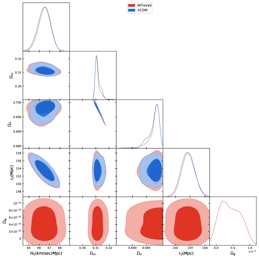
Model	$H_{0}(Km/sec/Mpc)$	$\Omega_{m}$	$\Omega_{\Lambda}$	$\Omega_{\phi}(10^{-25})$	$r_{s}(Mpc)$	$\Delta B_{ij}$
MiTeVeS	$66.52\pm 0.532$	$0.31\pm 0.021$	$0.698\pm 0.019$	$4.258\pm 2.87$	$153.2\pm 1.69$	$0.24$
$\Lambda$CDM	$66.58\pm 0.47$	$0.311\pm 0.016$	$0.698\pm 0.01$	-	$153.3\pm 1.465$	-

Figure 1: The posterior distribution for the simplest case of the MiTeVeS with constant functions (red curve) and for $\Lambda$CDM model (blue curve). The ratios of the matter density $\Omega_{m}$, dark energy $\Omega_{\Lambda}$, radiation density $\Omega_{r}$ and the stiff part $\Omega_{\phi}$ summarize to one. The final results for cosmological parameters for the MiTeVeS and the $\Lambda$CDM models are summarized in the table. In order to compare the models we calculate the Bayes factor.

VI Cosmological Constraints

In order to constrain the additional equation of state we use standard candles (SCs), Baryon Acoustic Oscillations (BAO) and the Cosmic Microwave Background (CMB) distance priors (three data points that contain information of certain features of the power spectrum such as the position of a peak). Radiation is included in order to constraint the components also in the early universe. The normalized Hubble function reads:

$$\left(\frac{H(z)}{H_{0}}\right)^{2}=\Omega_{\Lambda}+\Omega_{m}(1+z)^{3}+\Omega_{r}(1+z)^{4}+\Omega_{\phi}(1+z)^{6}.$$ (59)

where $H_{0}$ is the current value of the Hubble parameter, and the other constants related to the MiTeVeS model are

$$\begin{split}\Omega_{\phi}=\frac{C^{2}_{0}}{6H_{0}^{2}},\quad\Omega_{m}=\frac{C_{0}h_{2}}{3\sqrt{f}H_{0}^{2}}+\Omega_{b},\\ \Omega_{\Lambda}=\frac{V}{3H_{0}^{2}}+\frac{h_{2}^{2}-4h_{1}}{24fH_{0}^{2}},\end{split}$$ (60)

where $\Omega_{\phi}$ is the density parameter of the stiff matter, $\Omega_{m}$ is the density parameter of usual matter and dark matter, and $\Omega_{\Lambda}$ is the density parameter of dark energy. $\Omega_{r}$ is the density parameter of radiation. The matter density incorporates the dark matter density from the MiTeVeS fields as $C_{0}h_{2}/3\sqrt{f}H_{0}^{2}$ and the density of baryons $\Omega_{b}$.

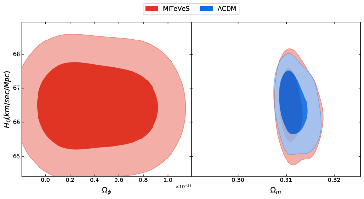
Figure 2: The posterior distribution for the simplest case of the MiTeVeS with constant functions (red curve) and for $\Lambda$CDM model (blue curve), with $H_{0}$ vs. $\Omega_{m}$.

In order to constrain our model, we use a few data sets. First we impose the average bound on the possible variation of the Big Bang Nucleosynthesis (BBN) speed-up factor, defined as the ratio of the expansion rate predicted in a given model versus that of the $\Lambda$CDM model at the BBN epoch ($z_{BBN}\sim 10^{9}$). This amounts to the limit Uzan (2011) with $\left({\Delta H}/{H_{\Lambda CDM}}\right)^{2}<0.01$, where $H_{\Lambda CDM}$ is the Hubble rate for the $\Lambda$CDM model and the $\Delta H$ is the difference between the MiTeVeS Hubble rate and the $\Lambda$CDM Hubble rate, $\Delta H=H-H_{\Lambda CDM}$. Imposing the relation (59) gives a bound on $\Omega_{\phi}$:

$$\Omega_{\phi}(Max)=\frac{\Omega_{\Lambda}+\Omega_{m}(1+z_{BBN})^{3}+\Omega_{r}(1+z_{BBN})^{4}}{100(1+z_{BBN})^{6}},$$ (61)

which gives a range of $10^{-22}$–$10^{-30}$ for the Planck values of $\Omega_{m}$ and $\Omega_{\Lambda}$. Therefore we set the value of $\Omega_{\phi}$ during BBN to be between zero and $\Omega_{\phi}(Max)$.

The Cosmic Chronometers (CC) exploit the evolution of differential ages of passive galaxies at different redshifts to directly constrain the Hubble parameter Jimenez and Loeb (2002). We use uncorrelated 30 CC measurements of $H(z)$ discussed in Moresco et al. (2012a, b); Moresco (2015); Moresco et al. (2016).

For Standard Candles (SC) we use measurements of the Pantheon Type Ia supernova dataset Scolnic et al. (2018) from different binnes. The parameters of the model are fitted by comparing the observed value $\mu_{i}^{obs}$ to the theoretical value $\mu_{i}^{th}$ of the distance moduli, which is given by:

$$\mu=m-M=5\log_{10}(D_{L})+\mu_{0},$$ (62)

where $m$ and $M$ are the apparent and absolute magnitudes and $\mu_{0}=5\log\left(H_{0}^{-1}/Mpc\right)+25$ is the nuisance parameter that has been marginalized. The distance moduli is given for different redshifts $\mu_{i}=\mu(z_{i})$. The luminosity distance is defined by

$$D_{L}(z) = \frac{c}{H_{0}}(1+z)\int_{0}^{z}\frac{dz^{\ast}}{E(z^{\ast})}.$$ (63)

Here, we assume that $\Omega_{k}=0$ (flat space-time). We use uncorrelated data points from different Baryon Acoustic Oscillations (BAO) Percival et al. (2010); Beutler et al. (2011); Busca et al. (2013); Anderson et al. (2013); Seo et al. (2012); Ross et al. (2015); Tojeiro et al. (2014); Bautista et al. (2018); de Carvalho et al. (2018); Ata et al. (2018); Abbott et al. (2019); Molavi and Khodam-Mohammadi (2019). Studies of the BAO feature in the transverse direction provide a measurement of $D_{H}(z)/r_{d}=c/H(z)r_{d}$, where $r_{d}$ is the sound horizon at the drag epoch and it is taken as an independent parameter and with the comoving angular diameter distance being:

$$D_{M}=\int_{0}^{z}\frac{c\,dz^{\prime}}{H(z^{\prime})}.$$ (64)

In our database we also use the angular diameter distance $D_{A}=D_{M}/(1+z)$ and $D_{V}(z)/r_{d}$, which is a combination of the BAO peak coordinates above, namely

$$D_{V}(z)\equiv[zD_{H}(z)D_{M}^{2}(z)]^{1/3}.$$ (65)

The BAO data represent the absolute distance measurements in the Universe. From the measurements of correlation function or power spectrum of large scale structure, we can use the BAO signal to estimate the distance scales at different redshifts. The BAO data are analyzed based on a fiducial cosmology and the sound horizon at the drag epoch.

For the CMB data, we use the CMB shift parameters (Chen et al., 2019). The values of the shift parameters with the corresponding covariant forms are called the CMB distant priors. The parameters read:

$$R=\sqrt{\Omega_{m}}H_{0}r(z_{*})/c,\quad l_{a}=\pi r(z_{*})/r_{s}(z_{*}),$$ (66)

which are based on the Planck data release (Aghanim et al., 2020). where $r_{s}(z)$ is the comoving sound horizon and $z_{*}$ is the redshift with respect to the photon-decoupling surface. The comoving sound horizon is defined as

$$r_{s}(z)=\frac{c}{H_{0}}\int_{0}^{a}\frac{da^{\prime}}{\sqrt{3(1+\bar{R_{b}}a^{\prime})a^{\prime 4}E^{2}(z^{\prime})}}.$$ (67)

It is determined by the matter-radiation equality relation and $z_{\text{eq}}=2.5\times 10^{4}\Omega_{m}h^{2}(T_{\text{CMB}}/2.7\text{K})^{-4}$ and with $\bar{R_{b}}=31500w_{b}(T_{\text{CMB}}/2.7\,\text{K})^{-4}$, where the CMB temperature is $T_{\text{CMB}}=2.7255\,\text{K}$.

Regarding the problem of likelihood maximization, we use an affine-invariant Markov Chain Monte Carlo (MCMC) sampler, as it is implemented within the open-source package Polychord Handley et al. (2015) with the GetDist package Lewis (2019) to present the results. The prior we choose is with a uniform distribution, where $\Omega_{m}\in[0.;1.]$, $\Omega_{\Lambda}\in[0.;1-\Omega_{m}]$, $\Omega_{\phi}\in[0.;1-\Omega_{m}-\Omega_{\Lambda}]$, $\Omega_{\phi}\in[0.;1-\Omega_{\phi}(Max)]$, $\Omega_{r}\in[0.;1-\Omega_{m}-\Omega_{\Lambda}-\Omega_{\phi}]$, $H_{0}\in[50;100]$ km/sec/Mpc. For the baryonic matter we use the value reported by Planck 2018.

The posterior distribution is presented in Fig. 1, which describes the best fit of the MCMC analysis. The differences between the parameters of MiTeVeS and $\Lambda$CDM are rather small. For the MiTeVeS the Hubble parameter is $66.52\pm 0.53$ km/sec/Mpc and for the $\Lambda$CDM model $66.58\pm 0.47$ km/sec/Mpc. The matter density is $0.31\pm 0.021$ for MiTeVeS and $0.311\pm 0.016$ for $\Lambda$CDM. The dark energy density is $0.698\pm 0.019$ for MiTeVeS and $0.698\pm 0.01$ for the $\Lambda$CDM model. Because of the error bars of all of these parameters, one cannot distinguish the difference from the current cosmological measurements. However, according to current measurements, the stiff matter may exist in our Universe, but its density portion is constrained to be of order $10^{-25}$ or smaller. To be more precise, the MCMC gives:

$$\Omega_{\phi}=\left(4.258\pm 2.877\right)\cdot 10^{-25}.$$ (68)

The value is compatible with zero with $2\sigma$. In order to test the preference of the models, we use the Bayesian Evidence that is calculated from the Polychord directly Kass and Raftery (1995). The difference between the Bayesian Evidence yields $0.24$, which is an indistinguishable preference for the $\Lambda$CDM model.

Although the value of the stiff matter density $\Omega_{\phi}$ has to be very small in order to be consistent with the cosmological observations, being constrained below a maximum value during BBN (61) and having the present value (68) in our model, stiff matter may play a role in the very early universe. Also it could be interesting to mention that a cosmological fluid with the stiff equation of state appears in gravitational theories where the connection has torsion Lucat and Prokopec (2017); Unger and Popławski (2019); Medina et al. (2019). Torsion appears in several types of gravitational theories, such as in the Einstein-Cartan and the gauge theories of gravity (for some comprehensive reviews, see, e.g. Hehl et al. (1995); Blagojević and Hehl (2013) and the references therein) as well as in supergravity (see for example Van Nieuwenhuizen (1981)). If the stiff fluid has a negative energy density, which is the the case for example in the Einstein-Cartan theory of gravity Medina et al. (2019), there is no initial singularity Chavanis (2015); Trautman (1973), since the scale factor remains nonzero at the beginning. In our model, when there are no interactions between stiff matter, dark matter and dark energy due to the choice of constant functions (52), the energy density of stiff matter is positive (57), and hence the initial singularity exists Chavanis (2015) similarly as in the $\Lambda$CDM model.

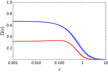
Figure 3: The evolution of the $\Omega_{m}$ (red) and $V(\phi)=\Omega_{\Lambda}$ (blue) for low and high redshifts, without any interaction (smooth line) or with interaction where $\beta=1$ (smooth line).

VII Interacting dark energy and dark matter

In this section we discuss the further possibilities of the MiTeVeS theory with general interaction forms. For the solution discussed in sections V and VI the mimetic dark matter component is not distinguishable from dust at the background level. However, for nonconstant functions (Eq. 52) one can get interacting dynamical dark energy and dark matter, which emerges naturally from the MiTeVeS action.

In order to track the evolution of the Universe (numerically and analytically) in the general case we rewrite the field equations in terms of the redshift instead of time, which is done using the relation:

$$\frac{d}{dt}=-H(z)\left(1+z\right)\frac{d}{dz}.$$ (69)

The modified scalar field equation is given as:

$$\begin{split}\phi^{\prime}(z)\left((z+1)\frac{H^{\prime}(z)}{H}-(3\tilde{h}(\phi)+2)\right)\\ +(z+1)\phi^{\prime\prime}(z)+\frac{V^{\prime}(\phi)}{(z+1)H^{2}}=0,\end{split}$$ (70)

where $H=H(z)$ and $\phi=\phi(z)$ are functions of the redshift. In principle, we need two equations to describe the full evolution. Equations (51b) and (51c) describe the evolution of $\phi(z)$ and $E(z)=H(z)/H_{0}$:

$$\begin{split}E^{\prime}(z)&=\frac{3}{2}\tilde{h}(\phi)\phi^{\prime}(z)\\ &+\frac{3E(z)^{2}-3\tilde{V}(\phi)-1.5\Omega_{m}(z)+1.5\Omega_{p}(z)}{E(z)(1+z)},\end{split}$$ (71a)

$$\phi^{\prime}(z)^{2}=\frac{E(z)^{2}-\tilde{V}(\phi)-\Omega_{m}(z)}{(1+z)^{2}E(z)^{2}},$$ (71b)

where $\Omega_{m}(z)=\rho_{m}/3H_{0}^{2}$ and $\Omega_{p}(z)=p_{m}/3H_{0}^{2}$. In order to determine the evolution of the variables for a general form of the functions, $E(z)$ and $\phi(z)$ are evaluated via these two equations. For the case $\tilde{h}(z)=0$ the system recovers to the standard solution, where $\dot{\phi}^{2}\sim(1+z)^{-3}$.

A nonconstant function $\tilde{h}(\phi)$ can give an interaction between dark energy and dark matter. As an example we take: $\tilde{h}(\phi)=\beta\phi$. The numerical evaluation of the matter density (in red) and the dark energy density (in blue) is described in Fig. 3. The smooth line shows the evaluation without any interaction and the dashed line shows the evaluation with interaction, where we assume $\beta=1$ and $\phi(z=0)=0$ for simplicity. The interaction changes the rates between the dark energy and dark matter. The possibility for such an interaction appears naturally in the MiTeVeS action.

VIII Discussion and conclusion

In this paper we have uncovered some cosmological implications of the MiTeVeS theory. The particular formulation of the theory includes both a scalar field and a vector field, which is stable and free from ghosts. The two simplest interactions between the scalar field and the vector field were considered. In the homogeneous FLRW background, the first interaction in (9) results only to a redefinition of the potential of the scalar field (50). However, the second interaction in (9) has interesting cosmological implications. For constant functions (52), a conserved Noether current emerges. From the scalar field dynamics, we obtained dark energy, dark matter and stiff matter. When the shift symmetry is broken, the current is not covariantly conserved. Consequently, possible interactions between these three components emerge.

We use the latest observations of the Big Bang Nucleosynthesis, Cosmic Chronometers, Type Ia Supernova, Baryon Acoustic Oscillations and the Cosmic Microwave Background distant prior to constrain the additional stiff matter contribution, which is not present in the standard $\Lambda$CDM model. It is clear that the dynamics of the Universe does not change significantly as long as the energy density of the stiff matter part is around $10^{-25}$ or smaller.

There are a few directions to continue the research. It is possible to explore different potentials and functions that approach constant functions asymptotically. We show one simple example of an interaction that changes the rates between dark energy and dark matter naturally from the action, which could be investigated in the future. Such functions produce interaction between the stiff matter, the dark matter and the dark energy parts, and may resolve the cosmic tensions regarding $H_{0}$ and others. Moreover, it is important to track the perturbation solutions for this theory in order to compare with further data sets and to validate the formulation in different systems.

The third interesting option is to explore the effect of the scalar $\Phi$ in this theory. This scalar is suggested in the theory and gives the behavior of dynamical $G\sim\Phi^{-2}$. Many versions of MOND and other modified theories of gravity suggest this effect that naturally emerges in this formulation. So the full theory gives additional effect of emerging gravity that should be studied in the future.