Abstract
The scalar field of extremal space-time film is considered as unified fundamental field.
Metrical interaction between solitons-particles as gravitational interaction is considered here in approximation of a weak fundamental field.
It is shown that the signature of metrics { − , + , + , + } \{-,+,+,+\}
1 Introduction
We consider the scalar field of space-time film as unified fundamental field [1 ] .
This scalar field model is related to well known Born – Infeld nonlinear electrodynamics [2 , 3 ] .
The model under consideration is attractive because it has relatively simple and geometrically clear form.
It can be considered as a relativistic generalization of the minimal surface or
minimal thin film model in three-dimensional space.
The model under consideration provides the necessary effects which are required for a realistic unified filed model.
In particular, there are exact solutions of the model equation which can be considered as photons [4 ] .
Also, in the space-time film theory, distant interactions of two kinds between particles-solitons, namely force and metrical interactions [5 ] , correspond to electromagnetic [6 ] and gravitational [7 ] interactions of particles respectively.
Here we apply the induced gravitational interaction in the framework of the space-time film theory [8 ] to stars in a galaxy. So we try to solve the known so called dark matter problem.
2 Extremal space-time film
The following variational principle and the action which has the world volume form are considered:
δ 𝒜 = 0 , 𝒜 = ∫ V ¯ | 𝔐 | ( d x ) 4 = ∫ V ¯ − ℒ d V ¯ , formulae-sequence 𝛿 𝒜 0 𝒜 subscript ¯ 𝑉 𝔐 superscript d 𝑥 4 subscript ¯ 𝑉 ℒ d ¯ 𝑉 \delta\mathcal{A}=0\;,\qquad\mathcal{A}=\int_{\overline{V}}\!\sqrt{|\mathfrak{M}|}\;(\mathrm{d}x)^{4}=\int_{\overline{V}}\mathchoice{{\hbox to0.0pt{\raisebox{1.29167pt}{${\scriptstyle-}$}\hss}}\mathcal{L}}{{\hbox to0.0pt{\raisebox{1.29167pt}{${\scriptstyle-}$}\hss}}\mathcal{L}}{{\hbox to0.0pt{\raisebox{1.07639pt}{${\scriptscriptstyle-}$}\hss}}\mathcal{L}}{}{}\;\mathrm{d}\mspace{-2.0mu}\overline{V}\;, (1a)
where 𝔐 ≑ det ( 𝔐 μ ν ) geometrically-equals 𝔐 subscript 𝔐 𝜇 𝜈 \mathfrak{M}\doteqdot\det(\mathfrak{M}_{\mu\nu}) ( d x ) 4 ≑ d x 0 d x 1 d x 2 d x 3 geometrically-equals superscript d 𝑥 4 d superscript 𝑥 0 d superscript 𝑥 1 d superscript 𝑥 2 d superscript 𝑥 3 \left(\mathrm{d}x\right)^{4}\doteqdot\mathrm{d}x^{0}\mathrm{d}x^{1}\mathrm{d}x^{2}\mathrm{d}x^{3} V ¯ ¯ 𝑉 \overline{V} d V ¯ ≑ | 𝔪 | ( d x ) 4 geometrically-equals d ¯ 𝑉 𝔪 superscript d 𝑥 4 \mathrm{d}\mspace{-2.0mu}\overline{V}\doteqdot\sqrt{|\mathfrak{m}|}\;\left(\mathrm{d}x\right)^{4}
𝔐 μ ν = 𝔪 μ ν + χ 2 ∂ Φ ∂ x μ ∂ Φ ∂ x ν , − ℒ ≑ | 1 + χ 2 𝔪 μ ν ∂ Φ ∂ x μ ∂ Φ ∂ x ν | formulae-sequence subscript 𝔐 𝜇 𝜈 subscript 𝔪 𝜇 𝜈 superscript 𝜒 2 Φ superscript 𝑥 𝜇 Φ superscript 𝑥 𝜈 geometrically-equals ℒ 1 superscript 𝜒 2 superscript 𝔪 𝜇 𝜈 Φ superscript 𝑥 𝜇 Φ superscript 𝑥 𝜈 \mathfrak{M}_{\mu\nu}=\mathfrak{m}_{\mu\nu}+\chi^{2}\,\frac{\partial\Phi}{\partial x^{\mu}}\,\frac{\partial\Phi}{\partial x^{\nu}}\;,\qquad\mathchoice{{\hbox to0.0pt{\raisebox{1.29167pt}{${\scriptstyle-}$}\hss}}\mathcal{L}}{{\hbox to0.0pt{\raisebox{1.29167pt}{${\scriptstyle-}$}\hss}}\mathcal{L}}{{\hbox to0.0pt{\raisebox{1.07639pt}{${\scriptscriptstyle-}$}\hss}}\mathcal{L}}{}{}\doteqdot\sqrt{\left|1+\chi^{2}\,\mathfrak{m}^{\mu\nu}\,\frac{\partial\Phi}{\partial x^{\mu}}\,\frac{\partial\Phi}{\partial x^{\nu}}\right|} (1b)
𝔪 μ ν subscript 𝔪 𝜇 𝜈 \mathfrak{m}_{\mu\nu} Φ Φ \Phi χ 𝜒 \chi { 0 , 1 , 2 , 3 } 0 1 2 3 \{0,1,2,3\} 𝔐 μ ν subscript 𝔐 𝜇 𝜈 \mathfrak{M}_{\mu\nu}
The model (1
We consider two possible signatures of metrics in the expression of Lagrangian (1b { + , − , − , − } \{+,-,-,-\} { − , + , + , + } \{-,+,+,+\} { − , + , + , + } \{-,+,+,+\} 1b
We have the following symmetrical canonical energy-momentum density tensor of the model in
Cartesian coordinates
− → T μ ν = 1 4 π ( Φ μ Φ ν − ℒ − − 𝔪 μ ν χ 2 − ℒ ) , Φ α ≑ − 𝔪 ∂ Φ ∂ x β α β . \mathchoice{{\hbox to0.0pt{\hskip 0.86108pt\raisebox{6.45831pt}{${\scriptstyle-}$}\hss}}{\mathchoice{{\hbox to0.0pt{\raisebox{1.29167pt}{${\scriptstyle\to}$}\hss}}{T}}{{\hbox to0.0pt{\raisebox{1.29167pt}{${\scriptstyle\to}$}\hss}}{T}}{{\hbox to0.0pt{\raisebox{0.86108pt}{${\scriptscriptstyle\to}$}\hss}}{T}}{{\hbox to0.0pt{\raisebox{0.86108pt}{${\scriptscriptstyle\to}$}\hss}}{T}}}}{{\hbox to0.0pt{\hskip 0.86108pt\raisebox{6.45831pt}{${\scriptstyle-}$}\hss}}{\mathchoice{{\hbox to0.0pt{\raisebox{1.29167pt}{${\scriptstyle\to}$}\hss}}{T}}{{\hbox to0.0pt{\raisebox{1.29167pt}{${\scriptstyle\to}$}\hss}}{T}}{{\hbox to0.0pt{\raisebox{0.86108pt}{${\scriptscriptstyle\to}$}\hss}}{T}}{{\hbox to0.0pt{\raisebox{0.86108pt}{${\scriptscriptstyle\to}$}\hss}}{T}}}}{{\hbox to0.0pt{\hskip 0.21529pt\raisebox{4.73611pt}{${\scriptscriptstyle-}$}\hss}}{\mathchoice{{\hbox to0.0pt{\raisebox{1.29167pt}{${\scriptstyle\to}$}\hss}}{T}}{{\hbox to0.0pt{\raisebox{1.29167pt}{${\scriptstyle\to}$}\hss}}{T}}{{\hbox to0.0pt{\raisebox{0.86108pt}{${\scriptscriptstyle\to}$}\hss}}{T}}{{\hbox to0.0pt{\raisebox{0.86108pt}{${\scriptscriptstyle\to}$}\hss}}{T}}}}{{\hbox to0.0pt{\hskip 0.21529pt\raisebox{4.73611pt}{${\scriptscriptstyle-}$}\hss}}{\mathchoice{{\hbox to0.0pt{\raisebox{1.29167pt}{${\scriptstyle\to}$}\hss}}{T}}{{\hbox to0.0pt{\raisebox{1.29167pt}{${\scriptstyle\to}$}\hss}}{T}}{{\hbox to0.0pt{\raisebox{0.86108pt}{${\scriptscriptstyle\to}$}\hss}}{T}}{{\hbox to0.0pt{\raisebox{0.86108pt}{${\scriptscriptstyle\to}$}\hss}}{T}}}}^{\mu\nu}=\frac{1}{4\pi}\left(\frac{\Phi^{\mu}\,\Phi^{\nu}}{\mathchoice{{\hbox to0.0pt{\raisebox{1.29167pt}{${\scriptstyle-}$}\hss}}\mathcal{L}}{{\hbox to0.0pt{\raisebox{1.29167pt}{${\scriptstyle-}$}\hss}}\mathcal{L}}{{\hbox to0.0pt{\raisebox{1.07639pt}{${\scriptscriptstyle-}$}\hss}}\mathcal{L}}{}{}}-\frac{\mathchoice{{\hbox to0.0pt{\raisebox{-3.87495pt}{${-}$}\hss}}\mathfrak{m}}{{\hbox to0.0pt{\raisebox{-3.87495pt}{${-}$}\hss}}\mathfrak{m}}{{\hbox to0.0pt{\raisebox{-3.22916pt}{${\scriptstyle-}$}\hss}}\mathfrak{m}}{}{}^{\mu\nu}}{\chi^{2}}\,\mathchoice{{\hbox to0.0pt{\raisebox{1.29167pt}{${\scriptstyle-}$}\hss}}\mathcal{L}}{{\hbox to0.0pt{\raisebox{1.29167pt}{${\scriptstyle-}$}\hss}}\mathcal{L}}{{\hbox to0.0pt{\raisebox{1.07639pt}{${\scriptscriptstyle-}$}\hss}}\mathcal{L}}{}{}\right)\;,\quad\Phi^{\alpha}\doteqdot\mathchoice{{\hbox to0.0pt{\raisebox{-3.87495pt}{${-}$}\hss}}\mathfrak{m}}{{\hbox to0.0pt{\raisebox{-3.87495pt}{${-}$}\hss}}\mathfrak{m}}{{\hbox to0.0pt{\raisebox{-3.22916pt}{${\scriptstyle-}$}\hss}}\mathfrak{m}}{}{}^{\alpha\beta}\,\frac{\partial\Phi}{\partial x^{\beta}}\;. (2)
where − 𝔪 μ ν \mathchoice{{\hbox to0.0pt{\raisebox{-3.87495pt}{${-}$}\hss}}\mathfrak{m}}{{\hbox to0.0pt{\raisebox{-3.87495pt}{${-}$}\hss}}\mathfrak{m}}{{\hbox to0.0pt{\raisebox{-3.22916pt}{${\scriptstyle-}$}\hss}}\mathfrak{m}}{}{}^{\mu\nu}
To use finite integral characteristics of solutions in infinite space-time we introduce regularized energy-momentum density tensor with the following formula:
→ T μ ν = − → T μ ν − ∞ → T μ ν , ∞ → T μ ν = − 1 4 π χ 2 − 𝔪 . μ ν \mathchoice{{\hbox to0.0pt{\raisebox{1.29167pt}{${\scriptstyle\to}$}\hss}}{T}}{{\hbox to0.0pt{\raisebox{1.29167pt}{${\scriptstyle\to}$}\hss}}{T}}{{\hbox to0.0pt{\raisebox{0.86108pt}{${\scriptscriptstyle\to}$}\hss}}{T}}{{\hbox to0.0pt{\raisebox{0.86108pt}{${\scriptscriptstyle\to}$}\hss}}{T}}^{\mu\nu}=\mathchoice{{\hbox to0.0pt{\hskip 0.86108pt\raisebox{6.45831pt}{${\scriptstyle-}$}\hss}}{\mathchoice{{\hbox to0.0pt{\raisebox{1.29167pt}{${\scriptstyle\to}$}\hss}}{T}}{{\hbox to0.0pt{\raisebox{1.29167pt}{${\scriptstyle\to}$}\hss}}{T}}{{\hbox to0.0pt{\raisebox{0.86108pt}{${\scriptscriptstyle\to}$}\hss}}{T}}{{\hbox to0.0pt{\raisebox{0.86108pt}{${\scriptscriptstyle\to}$}\hss}}{T}}}}{{\hbox to0.0pt{\hskip 0.86108pt\raisebox{6.45831pt}{${\scriptstyle-}$}\hss}}{\mathchoice{{\hbox to0.0pt{\raisebox{1.29167pt}{${\scriptstyle\to}$}\hss}}{T}}{{\hbox to0.0pt{\raisebox{1.29167pt}{${\scriptstyle\to}$}\hss}}{T}}{{\hbox to0.0pt{\raisebox{0.86108pt}{${\scriptscriptstyle\to}$}\hss}}{T}}{{\hbox to0.0pt{\raisebox{0.86108pt}{${\scriptscriptstyle\to}$}\hss}}{T}}}}{{\hbox to0.0pt{\hskip 0.21529pt\raisebox{4.73611pt}{${\scriptscriptstyle-}$}\hss}}{\mathchoice{{\hbox to0.0pt{\raisebox{1.29167pt}{${\scriptstyle\to}$}\hss}}{T}}{{\hbox to0.0pt{\raisebox{1.29167pt}{${\scriptstyle\to}$}\hss}}{T}}{{\hbox to0.0pt{\raisebox{0.86108pt}{${\scriptscriptstyle\to}$}\hss}}{T}}{{\hbox to0.0pt{\raisebox{0.86108pt}{${\scriptscriptstyle\to}$}\hss}}{T}}}}{{\hbox to0.0pt{\hskip 0.21529pt\raisebox{4.73611pt}{${\scriptscriptstyle-}$}\hss}}{\mathchoice{{\hbox to0.0pt{\raisebox{1.29167pt}{${\scriptstyle\to}$}\hss}}{T}}{{\hbox to0.0pt{\raisebox{1.29167pt}{${\scriptstyle\to}$}\hss}}{T}}{{\hbox to0.0pt{\raisebox{0.86108pt}{${\scriptscriptstyle\to}$}\hss}}{T}}{{\hbox to0.0pt{\raisebox{0.86108pt}{${\scriptscriptstyle\to}$}\hss}}{T}}}}^{\mu\nu}-\mathchoice{{\hbox to0.0pt{\hskip 0.6458pt\raisebox{7.74998pt}{${\scriptscriptstyle\infty}$}\hss}}\mathchoice{{\hbox to0.0pt{\raisebox{1.29167pt}{${\scriptstyle\to}$}\hss}}{T}}{{\hbox to0.0pt{\raisebox{1.29167pt}{${\scriptstyle\to}$}\hss}}{T}}{{\hbox to0.0pt{\raisebox{0.86108pt}{${\scriptscriptstyle\to}$}\hss}}{T}}{{\hbox to0.0pt{\raisebox{0.86108pt}{${\scriptscriptstyle\to}$}\hss}}{T}}}{{\hbox to0.0pt{\hskip 0.6458pt\raisebox{7.96527pt}{${\scriptscriptstyle\infty}$}\hss}}\mathchoice{{\hbox to0.0pt{\raisebox{1.29167pt}{${\scriptstyle\to}$}\hss}}{T}}{{\hbox to0.0pt{\raisebox{1.29167pt}{${\scriptstyle\to}$}\hss}}{T}}{{\hbox to0.0pt{\raisebox{0.86108pt}{${\scriptscriptstyle\to}$}\hss}}{T}}{{\hbox to0.0pt{\raisebox{0.86108pt}{${\scriptscriptstyle\to}$}\hss}}{T}}}{{\hbox to0.0pt{\raisebox{5.38193pt}{${\scriptscriptstyle\infty}$}\hss}}\mathchoice{{\hbox to0.0pt{\raisebox{1.29167pt}{${\scriptstyle\to}$}\hss}}{T}}{{\hbox to0.0pt{\raisebox{1.29167pt}{${\scriptstyle\to}$}\hss}}{T}}{{\hbox to0.0pt{\raisebox{0.86108pt}{${\scriptscriptstyle\to}$}\hss}}{T}}{{\hbox to0.0pt{\raisebox{0.86108pt}{${\scriptscriptstyle\to}$}\hss}}{T}}}{{\hbox to0.0pt{\raisebox{5.16663pt}{${\scriptscriptstyle\infty}$}\hss}}\mathchoice{{\hbox to0.0pt{\raisebox{1.29167pt}{${\scriptstyle\to}$}\hss}}{T}}{{\hbox to0.0pt{\raisebox{1.29167pt}{${\scriptstyle\to}$}\hss}}{T}}{{\hbox to0.0pt{\raisebox{0.86108pt}{${\scriptscriptstyle\to}$}\hss}}{T}}{{\hbox to0.0pt{\raisebox{0.86108pt}{${\scriptscriptstyle\to}$}\hss}}{T}}}^{\mu\nu}\,,\qquad\mathchoice{{\hbox to0.0pt{\hskip 0.6458pt\raisebox{7.74998pt}{${\scriptscriptstyle\infty}$}\hss}}\mathchoice{{\hbox to0.0pt{\raisebox{1.29167pt}{${\scriptstyle\to}$}\hss}}{T}}{{\hbox to0.0pt{\raisebox{1.29167pt}{${\scriptstyle\to}$}\hss}}{T}}{{\hbox to0.0pt{\raisebox{0.86108pt}{${\scriptscriptstyle\to}$}\hss}}{T}}{{\hbox to0.0pt{\raisebox{0.86108pt}{${\scriptscriptstyle\to}$}\hss}}{T}}}{{\hbox to0.0pt{\hskip 0.6458pt\raisebox{7.96527pt}{${\scriptscriptstyle\infty}$}\hss}}\mathchoice{{\hbox to0.0pt{\raisebox{1.29167pt}{${\scriptstyle\to}$}\hss}}{T}}{{\hbox to0.0pt{\raisebox{1.29167pt}{${\scriptstyle\to}$}\hss}}{T}}{{\hbox to0.0pt{\raisebox{0.86108pt}{${\scriptscriptstyle\to}$}\hss}}{T}}{{\hbox to0.0pt{\raisebox{0.86108pt}{${\scriptscriptstyle\to}$}\hss}}{T}}}{{\hbox to0.0pt{\raisebox{5.38193pt}{${\scriptscriptstyle\infty}$}\hss}}\mathchoice{{\hbox to0.0pt{\raisebox{1.29167pt}{${\scriptstyle\to}$}\hss}}{T}}{{\hbox to0.0pt{\raisebox{1.29167pt}{${\scriptstyle\to}$}\hss}}{T}}{{\hbox to0.0pt{\raisebox{0.86108pt}{${\scriptscriptstyle\to}$}\hss}}{T}}{{\hbox to0.0pt{\raisebox{0.86108pt}{${\scriptscriptstyle\to}$}\hss}}{T}}}{{\hbox to0.0pt{\raisebox{5.16663pt}{${\scriptscriptstyle\infty}$}\hss}}\mathchoice{{\hbox to0.0pt{\raisebox{1.29167pt}{${\scriptstyle\to}$}\hss}}{T}}{{\hbox to0.0pt{\raisebox{1.29167pt}{${\scriptstyle\to}$}\hss}}{T}}{{\hbox to0.0pt{\raisebox{0.86108pt}{${\scriptscriptstyle\to}$}\hss}}{T}}{{\hbox to0.0pt{\raisebox{0.86108pt}{${\scriptscriptstyle\to}$}\hss}}{T}}}^{\mu\nu}=-\frac{1}{4\pi\,\chi^{2}}\,\mathchoice{{\hbox to0.0pt{\raisebox{-3.87495pt}{${-}$}\hss}}\mathfrak{m}}{{\hbox to0.0pt{\raisebox{-3.87495pt}{${-}$}\hss}}\mathfrak{m}}{{\hbox to0.0pt{\raisebox{-3.22916pt}{${\scriptstyle-}$}\hss}}\mathfrak{m}}{}{}^{\mu\nu}\;. (3)
where ∞ → T μ ν ∞ → superscript 𝑇 𝜇 𝜈 \mathchoice{{\hbox to0.0pt{\hskip 0.6458pt\raisebox{7.74998pt}{${\scriptscriptstyle\infty}$}\hss}}\mathchoice{{\hbox to0.0pt{\raisebox{1.29167pt}{${\scriptstyle\to}$}\hss}}{T}}{{\hbox to0.0pt{\raisebox{1.29167pt}{${\scriptstyle\to}$}\hss}}{T}}{{\hbox to0.0pt{\raisebox{0.86108pt}{${\scriptscriptstyle\to}$}\hss}}{T}}{{\hbox to0.0pt{\raisebox{0.86108pt}{${\scriptscriptstyle\to}$}\hss}}{T}}}{{\hbox to0.0pt{\hskip 0.6458pt\raisebox{7.96527pt}{${\scriptscriptstyle\infty}$}\hss}}\mathchoice{{\hbox to0.0pt{\raisebox{1.29167pt}{${\scriptstyle\to}$}\hss}}{T}}{{\hbox to0.0pt{\raisebox{1.29167pt}{${\scriptstyle\to}$}\hss}}{T}}{{\hbox to0.0pt{\raisebox{0.86108pt}{${\scriptscriptstyle\to}$}\hss}}{T}}{{\hbox to0.0pt{\raisebox{0.86108pt}{${\scriptscriptstyle\to}$}\hss}}{T}}}{{\hbox to0.0pt{\raisebox{5.38193pt}{${\scriptscriptstyle\infty}$}\hss}}\mathchoice{{\hbox to0.0pt{\raisebox{1.29167pt}{${\scriptstyle\to}$}\hss}}{T}}{{\hbox to0.0pt{\raisebox{1.29167pt}{${\scriptstyle\to}$}\hss}}{T}}{{\hbox to0.0pt{\raisebox{0.86108pt}{${\scriptscriptstyle\to}$}\hss}}{T}}{{\hbox to0.0pt{\raisebox{0.86108pt}{${\scriptscriptstyle\to}$}\hss}}{T}}}{{\hbox to0.0pt{\raisebox{5.16663pt}{${\scriptscriptstyle\infty}$}\hss}}\mathchoice{{\hbox to0.0pt{\raisebox{1.29167pt}{${\scriptstyle\to}$}\hss}}{T}}{{\hbox to0.0pt{\raisebox{1.29167pt}{${\scriptstyle\to}$}\hss}}{T}}{{\hbox to0.0pt{\raisebox{0.86108pt}{${\scriptscriptstyle\to}$}\hss}}{T}}{{\hbox to0.0pt{\raisebox{0.86108pt}{${\scriptscriptstyle\to}$}\hss}}{T}}}^{\mu\nu}
The field equation in Cartesian coordinates can be written in the following form:
− → T μ ν ∂ 2 Φ ∂ x μ ∂ x ν = 0 , − → superscript 𝑇 𝜇 𝜈 superscript 2 Φ superscript 𝑥 𝜇 superscript 𝑥 𝜈 0 \mathchoice{{\hbox to0.0pt{\hskip 0.86108pt\raisebox{6.45831pt}{${\scriptstyle-}$}\hss}}{\mathchoice{{\hbox to0.0pt{\raisebox{1.29167pt}{${\scriptstyle\to}$}\hss}}{T}}{{\hbox to0.0pt{\raisebox{1.29167pt}{${\scriptstyle\to}$}\hss}}{T}}{{\hbox to0.0pt{\raisebox{0.86108pt}{${\scriptscriptstyle\to}$}\hss}}{T}}{{\hbox to0.0pt{\raisebox{0.86108pt}{${\scriptscriptstyle\to}$}\hss}}{T}}}}{{\hbox to0.0pt{\hskip 0.86108pt\raisebox{6.45831pt}{${\scriptstyle-}$}\hss}}{\mathchoice{{\hbox to0.0pt{\raisebox{1.29167pt}{${\scriptstyle\to}$}\hss}}{T}}{{\hbox to0.0pt{\raisebox{1.29167pt}{${\scriptstyle\to}$}\hss}}{T}}{{\hbox to0.0pt{\raisebox{0.86108pt}{${\scriptscriptstyle\to}$}\hss}}{T}}{{\hbox to0.0pt{\raisebox{0.86108pt}{${\scriptscriptstyle\to}$}\hss}}{T}}}}{{\hbox to0.0pt{\hskip 0.21529pt\raisebox{4.73611pt}{${\scriptscriptstyle-}$}\hss}}{\mathchoice{{\hbox to0.0pt{\raisebox{1.29167pt}{${\scriptstyle\to}$}\hss}}{T}}{{\hbox to0.0pt{\raisebox{1.29167pt}{${\scriptstyle\to}$}\hss}}{T}}{{\hbox to0.0pt{\raisebox{0.86108pt}{${\scriptscriptstyle\to}$}\hss}}{T}}{{\hbox to0.0pt{\raisebox{0.86108pt}{${\scriptscriptstyle\to}$}\hss}}{T}}}}{{\hbox to0.0pt{\hskip 0.21529pt\raisebox{4.73611pt}{${\scriptscriptstyle-}$}\hss}}{\mathchoice{{\hbox to0.0pt{\raisebox{1.29167pt}{${\scriptstyle\to}$}\hss}}{T}}{{\hbox to0.0pt{\raisebox{1.29167pt}{${\scriptstyle\to}$}\hss}}{T}}{{\hbox to0.0pt{\raisebox{0.86108pt}{${\scriptscriptstyle\to}$}\hss}}{T}}{{\hbox to0.0pt{\raisebox{0.86108pt}{${\scriptscriptstyle\to}$}\hss}}{T}}}}^{\mu\nu}\frac{\partial^{2}\,\Phi}{\partial x^{\mu}\,\partial x^{\nu}}=0\;, (4a)
where − → T μ ν − → superscript 𝑇 𝜇 𝜈 \mathchoice{{\hbox to0.0pt{\hskip 0.86108pt\raisebox{6.45831pt}{${\scriptstyle-}$}\hss}}{\mathchoice{{\hbox to0.0pt{\raisebox{1.29167pt}{${\scriptstyle\to}$}\hss}}{T}}{{\hbox to0.0pt{\raisebox{1.29167pt}{${\scriptstyle\to}$}\hss}}{T}}{{\hbox to0.0pt{\raisebox{0.86108pt}{${\scriptscriptstyle\to}$}\hss}}{T}}{{\hbox to0.0pt{\raisebox{0.86108pt}{${\scriptscriptstyle\to}$}\hss}}{T}}}}{{\hbox to0.0pt{\hskip 0.86108pt\raisebox{6.45831pt}{${\scriptstyle-}$}\hss}}{\mathchoice{{\hbox to0.0pt{\raisebox{1.29167pt}{${\scriptstyle\to}$}\hss}}{T}}{{\hbox to0.0pt{\raisebox{1.29167pt}{${\scriptstyle\to}$}\hss}}{T}}{{\hbox to0.0pt{\raisebox{0.86108pt}{${\scriptscriptstyle\to}$}\hss}}{T}}{{\hbox to0.0pt{\raisebox{0.86108pt}{${\scriptscriptstyle\to}$}\hss}}{T}}}}{{\hbox to0.0pt{\hskip 0.21529pt\raisebox{4.73611pt}{${\scriptscriptstyle-}$}\hss}}{\mathchoice{{\hbox to0.0pt{\raisebox{1.29167pt}{${\scriptstyle\to}$}\hss}}{T}}{{\hbox to0.0pt{\raisebox{1.29167pt}{${\scriptstyle\to}$}\hss}}{T}}{{\hbox to0.0pt{\raisebox{0.86108pt}{${\scriptscriptstyle\to}$}\hss}}{T}}{{\hbox to0.0pt{\raisebox{0.86108pt}{${\scriptscriptstyle\to}$}\hss}}{T}}}}{{\hbox to0.0pt{\hskip 0.21529pt\raisebox{4.73611pt}{${\scriptscriptstyle-}$}\hss}}{\mathchoice{{\hbox to0.0pt{\raisebox{1.29167pt}{${\scriptstyle\to}$}\hss}}{T}}{{\hbox to0.0pt{\raisebox{1.29167pt}{${\scriptstyle\to}$}\hss}}{T}}{{\hbox to0.0pt{\raisebox{0.86108pt}{${\scriptscriptstyle\to}$}\hss}}{T}}{{\hbox to0.0pt{\raisebox{0.86108pt}{${\scriptscriptstyle\to}$}\hss}}{T}}}}^{\mu\nu} 2
By multiplying (4a ( − 4 π χ 2 − ℒ ) 4 𝜋 superscript 𝜒 2 ℒ (-4\pi\,\chi^{2}\,\mathchoice{{\hbox to0.0pt{\raisebox{1.29167pt}{${\scriptstyle-}$}\hss}}\mathcal{L}}{{\hbox to0.0pt{\raisebox{1.29167pt}{${\scriptstyle-}$}\hss}}\mathcal{L}}{{\hbox to0.0pt{\raisebox{1.07639pt}{${\scriptscriptstyle-}$}\hss}}\mathcal{L}}{}{})
( − 𝔪 ( 1 + χ 2 − 𝔪 Φ σ σ ρ Φ ρ ) μ ν − χ 2 Φ μ Φ ν ) ∂ 2 Φ ∂ x μ ∂ x ν = 0 . \left(\mathchoice{{\hbox to0.0pt{\raisebox{-3.87495pt}{${-}$}\hss}}\mathfrak{m}}{{\hbox to0.0pt{\raisebox{-3.87495pt}{${-}$}\hss}}\mathfrak{m}}{{\hbox to0.0pt{\raisebox{-3.22916pt}{${\scriptstyle-}$}\hss}}\mathfrak{m}}{}{}^{\mu\nu}\left(1+\chi^{2}\,\mathchoice{{\hbox to0.0pt{\raisebox{-3.87495pt}{${-}$}\hss}}\mathfrak{m}}{{\hbox to0.0pt{\raisebox{-3.87495pt}{${-}$}\hss}}\mathfrak{m}}{{\hbox to0.0pt{\raisebox{-3.22916pt}{${\scriptstyle-}$}\hss}}\mathfrak{m}}{}{}_{\sigma\rho}\,\Phi^{\sigma}\,\Phi^{\rho}\right)-\chi^{2}\,\Phi^{\mu}\,\Phi^{\nu}\right)\frac{\partial^{2}\,\Phi}{\partial x^{\mu}\,\partial x^{\nu}}=0\;. (4b)
Equation (4 χ = 0 𝜒 0 \chi=0
− 𝔪 ∂ 2 Φ ∂ x μ ∂ x ν μ ν = 0 . 𝔪 superscript superscript 2 Φ superscript 𝑥 𝜇 superscript 𝑥 𝜈 𝜇 𝜈 0 \mathchoice{{\hbox to0.0pt{\raisebox{-3.87495pt}{${-}$}\hss}}\mathfrak{m}}{{\hbox to0.0pt{\raisebox{-3.87495pt}{${-}$}\hss}}\mathfrak{m}}{{\hbox to0.0pt{\raisebox{-3.22916pt}{${\scriptstyle-}$}\hss}}\mathfrak{m}}{}{}^{\mu\nu}\frac{\partial^{2}\,\Phi}{\partial x^{\mu}\,\partial x^{\nu}}=0\;. (5)
The model under consideration have the following notable characteristic equation:
∼ 𝔪 ∂ 𝒮 ∂ x μ μ ν ∂ 𝒮 ∂ x ν = 0 , ∼ 𝔪 ≑ μ ν − 4 π χ 2 − → T μ ν , \mathchoice{{\hbox to0.0pt{\hskip 0.86108pt\raisebox{4.30554pt}{${\scriptstyle\sim}$}\hss}}\mathfrak{m}}{{\hbox to0.0pt{\hskip 0.86108pt\raisebox{4.30554pt}{${\scriptstyle\sim}$}\hss}}\mathfrak{m}}{{\hbox to0.0pt{\hskip 0.21529pt\raisebox{2.84166pt}{${\scriptscriptstyle\sim}$}\hss}}\mathfrak{m}}{}{}^{\mu\nu}\,\frac{\partial{\cal S}}{\partial x^{\mu}}\,\frac{\partial{\cal S}}{\partial x^{\nu}}=0\;,\quad\quad\quad\mathchoice{{\hbox to0.0pt{\hskip 0.86108pt\raisebox{4.30554pt}{${\scriptstyle\sim}$}\hss}}\mathfrak{m}}{{\hbox to0.0pt{\hskip 0.86108pt\raisebox{4.30554pt}{${\scriptstyle\sim}$}\hss}}\mathfrak{m}}{{\hbox to0.0pt{\hskip 0.21529pt\raisebox{2.84166pt}{${\scriptscriptstyle\sim}$}\hss}}\mathfrak{m}}{}{}^{\mu\nu}\doteqdot-4\pi\,\chi^{2}\,\mathchoice{{\hbox to0.0pt{\hskip 0.86108pt\raisebox{6.45831pt}{${\scriptstyle-}$}\hss}}{\mathchoice{{\hbox to0.0pt{\raisebox{1.29167pt}{${\scriptstyle\to}$}\hss}}{T}}{{\hbox to0.0pt{\raisebox{1.29167pt}{${\scriptstyle\to}$}\hss}}{T}}{{\hbox to0.0pt{\raisebox{0.86108pt}{${\scriptscriptstyle\to}$}\hss}}{T}}{{\hbox to0.0pt{\raisebox{0.86108pt}{${\scriptscriptstyle\to}$}\hss}}{T}}}}{{\hbox to0.0pt{\hskip 0.86108pt\raisebox{6.45831pt}{${\scriptstyle-}$}\hss}}{\mathchoice{{\hbox to0.0pt{\raisebox{1.29167pt}{${\scriptstyle\to}$}\hss}}{T}}{{\hbox to0.0pt{\raisebox{1.29167pt}{${\scriptstyle\to}$}\hss}}{T}}{{\hbox to0.0pt{\raisebox{0.86108pt}{${\scriptscriptstyle\to}$}\hss}}{T}}{{\hbox to0.0pt{\raisebox{0.86108pt}{${\scriptscriptstyle\to}$}\hss}}{T}}}}{{\hbox to0.0pt{\hskip 0.21529pt\raisebox{4.73611pt}{${\scriptscriptstyle-}$}\hss}}{\mathchoice{{\hbox to0.0pt{\raisebox{1.29167pt}{${\scriptstyle\to}$}\hss}}{T}}{{\hbox to0.0pt{\raisebox{1.29167pt}{${\scriptstyle\to}$}\hss}}{T}}{{\hbox to0.0pt{\raisebox{0.86108pt}{${\scriptscriptstyle\to}$}\hss}}{T}}{{\hbox to0.0pt{\raisebox{0.86108pt}{${\scriptscriptstyle\to}$}\hss}}{T}}}}{{\hbox to0.0pt{\hskip 0.21529pt\raisebox{4.73611pt}{${\scriptscriptstyle-}$}\hss}}{\mathchoice{{\hbox to0.0pt{\raisebox{1.29167pt}{${\scriptstyle\to}$}\hss}}{T}}{{\hbox to0.0pt{\raisebox{1.29167pt}{${\scriptstyle\to}$}\hss}}{T}}{{\hbox to0.0pt{\raisebox{0.86108pt}{${\scriptscriptstyle\to}$}\hss}}{T}}{{\hbox to0.0pt{\raisebox{0.86108pt}{${\scriptscriptstyle\to}$}\hss}}{T}}}}^{\mu\nu}\;, (6)
where ∼ 𝔪 μ ν \mathchoice{{\hbox to0.0pt{\hskip 0.86108pt\raisebox{4.30554pt}{${\scriptstyle\sim}$}\hss}}\mathfrak{m}}{{\hbox to0.0pt{\hskip 0.86108pt\raisebox{4.30554pt}{${\scriptstyle\sim}$}\hss}}\mathfrak{m}}{{\hbox to0.0pt{\hskip 0.21529pt\raisebox{2.84166pt}{${\scriptscriptstyle\sim}$}\hss}}\mathfrak{m}}{}{}^{\mu\nu} − → T μ ν − → superscript 𝑇 𝜇 𝜈 \mathchoice{{\hbox to0.0pt{\hskip 0.86108pt\raisebox{6.45831pt}{${\scriptstyle-}$}\hss}}{\mathchoice{{\hbox to0.0pt{\raisebox{1.29167pt}{${\scriptstyle\to}$}\hss}}{T}}{{\hbox to0.0pt{\raisebox{1.29167pt}{${\scriptstyle\to}$}\hss}}{T}}{{\hbox to0.0pt{\raisebox{0.86108pt}{${\scriptscriptstyle\to}$}\hss}}{T}}{{\hbox to0.0pt{\raisebox{0.86108pt}{${\scriptscriptstyle\to}$}\hss}}{T}}}}{{\hbox to0.0pt{\hskip 0.86108pt\raisebox{6.45831pt}{${\scriptstyle-}$}\hss}}{\mathchoice{{\hbox to0.0pt{\raisebox{1.29167pt}{${\scriptstyle\to}$}\hss}}{T}}{{\hbox to0.0pt{\raisebox{1.29167pt}{${\scriptstyle\to}$}\hss}}{T}}{{\hbox to0.0pt{\raisebox{0.86108pt}{${\scriptscriptstyle\to}$}\hss}}{T}}{{\hbox to0.0pt{\raisebox{0.86108pt}{${\scriptscriptstyle\to}$}\hss}}{T}}}}{{\hbox to0.0pt{\hskip 0.21529pt\raisebox{4.73611pt}{${\scriptscriptstyle-}$}\hss}}{\mathchoice{{\hbox to0.0pt{\raisebox{1.29167pt}{${\scriptstyle\to}$}\hss}}{T}}{{\hbox to0.0pt{\raisebox{1.29167pt}{${\scriptstyle\to}$}\hss}}{T}}{{\hbox to0.0pt{\raisebox{0.86108pt}{${\scriptscriptstyle\to}$}\hss}}{T}}{{\hbox to0.0pt{\raisebox{0.86108pt}{${\scriptscriptstyle\to}$}\hss}}{T}}}}{{\hbox to0.0pt{\hskip 0.21529pt\raisebox{4.73611pt}{${\scriptscriptstyle-}$}\hss}}{\mathchoice{{\hbox to0.0pt{\raisebox{1.29167pt}{${\scriptstyle\to}$}\hss}}{T}}{{\hbox to0.0pt{\raisebox{1.29167pt}{${\scriptstyle\to}$}\hss}}{T}}{{\hbox to0.0pt{\raisebox{0.86108pt}{${\scriptscriptstyle\to}$}\hss}}{T}}{{\hbox to0.0pt{\raisebox{0.86108pt}{${\scriptscriptstyle\to}$}\hss}}{T}}}}^{\mu\nu} 𝒮 = 0 𝒮 0 {\cal S}=0
3 Gravitation as metrical interaction of solitons-particles
We consider the solitons-particles of two kind. Luminal solitons-particles have the speed of light and subluminal solitons-particles have a subluminal speed.
For a subluminal soliton, there is an intrinsic coordinate system in which the soliton rests as a whole. A subluminal soliton has a form of standing wave in its intrinsic coordinate system in general case.
There are also such space localized solutions for the linear wave equation (5
Φ = a ⋅ r sin ( ⋅ ω ⋅ r ) sin ( ⋅ ω ⋅ x 0 ) , Φ 𝑎 ⋅ 𝑟 ⋅ 𝜔 ⋅ 𝑟 ⋅ 𝜔 ⋅ superscript 𝑥 0 \Phi=\frac{a}{{\hbox to0.0pt{\hskip 1.29167pt\raisebox{-3.87495pt}{${\cdot}$}\hss}}{r}}\sin({\hbox to0.0pt{\hskip 1.29167pt\raisebox{-3.87495pt}{${\cdot}$}\hss}}{\omega}\,{\hbox to0.0pt{\hskip 1.29167pt\raisebox{-3.87495pt}{${\cdot}$}\hss}}{r})\,\sin({\hbox to0.0pt{\hskip 1.29167pt\raisebox{-3.87495pt}{${\cdot}$}\hss}}{\omega}\,{\hbox to0.0pt{\hskip 1.29167pt\raisebox{-3.87495pt}{${\cdot}$}\hss}}{x}^{0})\;, (7)
where a 𝑎 a ⋅ ω ⋅ 𝜔 {\hbox to0.0pt{\hskip 1.29167pt\raisebox{-3.87495pt}{${\cdot}$}\hss}}{\omega}
For an arbitrary Cartesian coordinate system, the wave vector { k μ } subscript 𝑘 𝜇 \{k_{\mu}\}
| − 𝔪 k μ μ ν k ν | = ⋅ ω 2 . 𝔪 superscript subscript 𝑘 𝜇 𝜇 𝜈 subscript 𝑘 𝜈 ⋅ superscript 𝜔 2 \bigl{|}\mathchoice{{\hbox to0.0pt{\raisebox{-3.87495pt}{${-}$}\hss}}\mathfrak{m}}{{\hbox to0.0pt{\raisebox{-3.87495pt}{${-}$}\hss}}\mathfrak{m}}{{\hbox to0.0pt{\raisebox{-3.22916pt}{${\scriptstyle-}$}\hss}}\mathfrak{m}}{}{}^{\mu\nu}\,k_{\mu}\,k_{\nu}\bigr{|}={\hbox to0.0pt{\hskip 1.29167pt\raisebox{-3.87495pt}{${\cdot}$}\hss}}{\omega}^{2}\;. (8)
And
the dispersion relation (8
| ∼ 𝔪 k μ μ ν k ν | = ⋅ ω 2 , ∼ 𝔪 superscript subscript 𝑘 𝜇 𝜇 𝜈 subscript 𝑘 𝜈 ⋅ superscript 𝜔 2 \bigl{|}\mathchoice{{\hbox to0.0pt{\hskip 0.86108pt\raisebox{4.30554pt}{${\scriptstyle\sim}$}\hss}}\mathfrak{m}}{{\hbox to0.0pt{\hskip 0.86108pt\raisebox{4.30554pt}{${\scriptstyle\sim}$}\hss}}\mathfrak{m}}{{\hbox to0.0pt{\hskip 0.21529pt\raisebox{2.84166pt}{${\scriptscriptstyle\sim}$}\hss}}\mathfrak{m}}{}{}^{\mu\nu}\,k_{\mu}\,k_{\nu}\bigr{|}={\hbox to0.0pt{\hskip 1.29167pt\raisebox{-3.87495pt}{${\cdot}$}\hss}}{\omega}^{2}\;, (9)
where ∼ 𝔪 μ ν \mathchoice{{\hbox to0.0pt{\hskip 0.86108pt\raisebox{4.30554pt}{${\scriptstyle\sim}$}\hss}}\mathfrak{m}}{{\hbox to0.0pt{\hskip 0.86108pt\raisebox{4.30554pt}{${\scriptstyle\sim}$}\hss}}\mathfrak{m}}{{\hbox to0.0pt{\hskip 0.21529pt\raisebox{2.84166pt}{${\scriptscriptstyle\sim}$}\hss}}\mathfrak{m}}{}{}^{\mu\nu} 6 ∼ 𝔪 = μ ν ∼ 𝔪 ( x ρ ) μ ν \mathchoice{{\hbox to0.0pt{\hskip 0.86108pt\raisebox{4.30554pt}{${\scriptstyle\sim}$}\hss}}\mathfrak{m}}{{\hbox to0.0pt{\hskip 0.86108pt\raisebox{4.30554pt}{${\scriptstyle\sim}$}\hss}}\mathfrak{m}}{{\hbox to0.0pt{\hskip 0.21529pt\raisebox{2.84166pt}{${\scriptscriptstyle\sim}$}\hss}}\mathfrak{m}}{}{}^{\mu\nu}{}={}\mathchoice{{\hbox to0.0pt{\hskip 0.86108pt\raisebox{4.30554pt}{${\scriptstyle\sim}$}\hss}}\mathfrak{m}}{{\hbox to0.0pt{\hskip 0.86108pt\raisebox{4.30554pt}{${\scriptstyle\sim}$}\hss}}\mathfrak{m}}{{\hbox to0.0pt{\hskip 0.21529pt\raisebox{2.84166pt}{${\scriptscriptstyle\sim}$}\hss}}\mathfrak{m}}{}{}^{\mu\nu}(x^{\rho}) k ¯ μ = k ¯ μ ( x ρ ) subscript ¯ 𝑘 𝜇 subscript ¯ 𝑘 𝜇 superscript 𝑥 𝜌 \bar{k}_{\mu}{}={}\bar{k}_{\mu}(x^{\rho})
The modified dispersion relation (9 [8 ] :
d ⋅ u μ d 𝔰 + ∼ Γ ⋅ ν ρ μ u ⋅ ν u = ρ 0 , ⋅ u ≑ μ d ⋅ x μ d 𝔰 , ∼ Γ ≑ ν ρ μ 1 2 ∼ 𝔪 ( ∂ ∼ 𝔪 ˇ δ ν ∂ x ρ + ∂ ∼ 𝔪 ˇ δ ρ ∂ x ν − ∂ ∼ 𝔪 ˇ ν ρ ∂ x δ ) μ δ , {\displaystyle\frac{\mathrm{d}\mathchoice{{\hbox to0.0pt{\hskip 1.29167pt\raisebox{-0.43057pt}{${\boldsymbol{\cdot}}$}\hss}}u}{{\hbox to0.0pt{\hskip 1.29167pt\raisebox{-0.43057pt}{${\boldsymbol{\cdot}}$}\hss}}u}{{\hbox to0.0pt{\hskip 0.86108pt\raisebox{-0.21529pt}{${\scriptstyle\boldsymbol{\cdot}}$}\hss}}u}{}{}^{\mu}}{\mathrm{d}\mathfrak{s}}}{}+{}\mathchoice{{\hbox to0.0pt{\hskip 0.43057pt\raisebox{6.45831pt}{${\scriptstyle\sim}$}\hss}}\Gamma}{{\hbox to0.0pt{\hskip 0.43057pt\raisebox{6.45831pt}{${\scriptstyle\sim}$}\hss}}\Gamma}{{\hbox to0.0pt{\raisebox{4.95134pt}{${\scriptscriptstyle\sim}$}\hss}}\Gamma}{}{}^{\mu}_{\nu\rho}\,\mathchoice{{\hbox to0.0pt{\hskip 1.29167pt\raisebox{-0.43057pt}{${\boldsymbol{\cdot}}$}\hss}}u}{{\hbox to0.0pt{\hskip 1.29167pt\raisebox{-0.43057pt}{${\boldsymbol{\cdot}}$}\hss}}u}{{\hbox to0.0pt{\hskip 0.86108pt\raisebox{-0.21529pt}{${\scriptstyle\boldsymbol{\cdot}}$}\hss}}u}{}{}^{\nu}\,\mathchoice{{\hbox to0.0pt{\hskip 1.29167pt\raisebox{-0.43057pt}{${\boldsymbol{\cdot}}$}\hss}}u}{{\hbox to0.0pt{\hskip 1.29167pt\raisebox{-0.43057pt}{${\boldsymbol{\cdot}}$}\hss}}u}{{\hbox to0.0pt{\hskip 0.86108pt\raisebox{-0.21529pt}{${\scriptstyle\boldsymbol{\cdot}}$}\hss}}u}{}{}^{\rho}=0\;,\qquad\mathchoice{{\hbox to0.0pt{\hskip 1.29167pt\raisebox{-0.43057pt}{${\boldsymbol{\cdot}}$}\hss}}u}{{\hbox to0.0pt{\hskip 1.29167pt\raisebox{-0.43057pt}{${\boldsymbol{\cdot}}$}\hss}}u}{{\hbox to0.0pt{\hskip 0.86108pt\raisebox{-0.21529pt}{${\scriptstyle\boldsymbol{\cdot}}$}\hss}}u}{}{}^{\mu}\doteqdot{\displaystyle\frac{\mathrm{d}\mathchoice{{\hbox to0.0pt{\raisebox{-0.43057pt}{${\boldsymbol{\cdot}}$}\hss}}x}{{\hbox to0.0pt{\raisebox{-0.43057pt}{${\boldsymbol{\cdot}}$}\hss}}x}{{\hbox to0.0pt{\raisebox{-0.21529pt}{${\scriptstyle\boldsymbol{\cdot}}$}\hss}}x}{}{}^{\mu}}{\mathrm{d}\mathfrak{s}}}\;,\qquad\mathchoice{{\hbox to0.0pt{\hskip 0.43057pt\raisebox{6.45831pt}{${\scriptstyle\sim}$}\hss}}\Gamma}{{\hbox to0.0pt{\hskip 0.43057pt\raisebox{6.45831pt}{${\scriptstyle\sim}$}\hss}}\Gamma}{{\hbox to0.0pt{\raisebox{4.95134pt}{${\scriptscriptstyle\sim}$}\hss}}\Gamma}{}{}^{\mu}_{\nu\rho}\doteqdot{\displaystyle\frac{1}{2}}\,\mathchoice{{\hbox to0.0pt{\hskip 0.86108pt\raisebox{4.30554pt}{${\scriptstyle\sim}$}\hss}}\mathfrak{m}}{{\hbox to0.0pt{\hskip 0.86108pt\raisebox{4.30554pt}{${\scriptstyle\sim}$}\hss}}\mathfrak{m}}{{\hbox to0.0pt{\hskip 0.21529pt\raisebox{2.84166pt}{${\scriptscriptstyle\sim}$}\hss}}\mathfrak{m}}{}{}^{\mu\delta}\left({\displaystyle\frac{\partial\check{\mathchoice{{\hbox to0.0pt{\hskip 0.86108pt\raisebox{4.30554pt}{${\scriptstyle\sim}$}\hss}}\mathfrak{m}}{{\hbox to0.0pt{\hskip 0.86108pt\raisebox{4.30554pt}{${\scriptstyle\sim}$}\hss}}\mathfrak{m}}{{\hbox to0.0pt{\hskip 0.21529pt\raisebox{2.84166pt}{${\scriptscriptstyle\sim}$}\hss}}\mathfrak{m}}{}{}}_{\delta\nu}}{\partial x^{\rho}}}{}+{}{\displaystyle\frac{\partial\check{\mathchoice{{\hbox to0.0pt{\hskip 0.86108pt\raisebox{4.30554pt}{${\scriptstyle\sim}$}\hss}}\mathfrak{m}}{{\hbox to0.0pt{\hskip 0.86108pt\raisebox{4.30554pt}{${\scriptstyle\sim}$}\hss}}\mathfrak{m}}{{\hbox to0.0pt{\hskip 0.21529pt\raisebox{2.84166pt}{${\scriptscriptstyle\sim}$}\hss}}\mathfrak{m}}{}{}}_{\delta\rho}}{\partial x^{\nu}}}{}-{}{\displaystyle\frac{\partial\check{\mathchoice{{\hbox to0.0pt{\hskip 0.86108pt\raisebox{4.30554pt}{${\scriptstyle\sim}$}\hss}}\mathfrak{m}}{{\hbox to0.0pt{\hskip 0.86108pt\raisebox{4.30554pt}{${\scriptstyle\sim}$}\hss}}\mathfrak{m}}{{\hbox to0.0pt{\hskip 0.21529pt\raisebox{2.84166pt}{${\scriptscriptstyle\sim}$}\hss}}\mathfrak{m}}{}{}}_{\nu\rho}}{\partial x^{\delta}}}\right)\;, (10)
where ⋅ x = j ⋅ x ( x 0 ) j \mathchoice{{\hbox to0.0pt{\raisebox{-0.43057pt}{${\boldsymbol{\cdot}}$}\hss}}x}{{\hbox to0.0pt{\raisebox{-0.43057pt}{${\boldsymbol{\cdot}}$}\hss}}x}{{\hbox to0.0pt{\raisebox{-0.21529pt}{${\scriptstyle\boldsymbol{\cdot}}$}\hss}}x}{}{}^{j}=\mathchoice{{\hbox to0.0pt{\raisebox{-0.43057pt}{${\boldsymbol{\cdot}}$}\hss}}x}{{\hbox to0.0pt{\raisebox{-0.43057pt}{${\boldsymbol{\cdot}}$}\hss}}x}{{\hbox to0.0pt{\raisebox{-0.21529pt}{${\scriptstyle\boldsymbol{\cdot}}$}\hss}}x}{}{}^{j}(x^{0}) ⋅ x = 0 x 0 \mathchoice{{\hbox to0.0pt{\raisebox{-0.43057pt}{${\boldsymbol{\cdot}}$}\hss}}x}{{\hbox to0.0pt{\raisebox{-0.43057pt}{${\boldsymbol{\cdot}}$}\hss}}x}{{\hbox to0.0pt{\raisebox{-0.21529pt}{${\scriptstyle\boldsymbol{\cdot}}$}\hss}}x}{}{}^{0}=x^{0} ∼ 𝔪 ˇ μ ν subscript ˇ ∼ 𝔪 𝜇 𝜈 \check{\mathchoice{{\hbox to0.0pt{\hskip 0.86108pt\raisebox{4.30554pt}{${\scriptstyle\sim}$}\hss}}\mathfrak{m}}{{\hbox to0.0pt{\hskip 0.86108pt\raisebox{4.30554pt}{${\scriptstyle\sim}$}\hss}}\mathfrak{m}}{{\hbox to0.0pt{\hskip 0.21529pt\raisebox{2.84166pt}{${\scriptscriptstyle\sim}$}\hss}}\mathfrak{m}}{}{}}_{\mu\nu} ∼ 𝔪 μ ν \mathchoice{{\hbox to0.0pt{\hskip 0.86108pt\raisebox{4.30554pt}{${\scriptstyle\sim}$}\hss}}\mathfrak{m}}{{\hbox to0.0pt{\hskip 0.86108pt\raisebox{4.30554pt}{${\scriptstyle\sim}$}\hss}}\mathfrak{m}}{{\hbox to0.0pt{\hskip 0.21529pt\raisebox{2.84166pt}{${\scriptscriptstyle\sim}$}\hss}}\mathfrak{m}}{}{}^{\mu\nu} 𝔰 𝔰 \mathfrak{s}
d 𝔰 2 = | ∼ 𝔪 ˇ μ ν d ⋅ x d μ ⋅ x | ν . \mathrm{d}\mathfrak{s}^{2}{\,}={\,}\left|\check{\mathchoice{{\hbox to0.0pt{\hskip 0.86108pt\raisebox{4.30554pt}{${\scriptstyle\sim}$}\hss}}\mathfrak{m}}{{\hbox to0.0pt{\hskip 0.86108pt\raisebox{4.30554pt}{${\scriptstyle\sim}$}\hss}}\mathfrak{m}}{{\hbox to0.0pt{\hskip 0.21529pt\raisebox{2.84166pt}{${\scriptscriptstyle\sim}$}\hss}}\mathfrak{m}}{}{}}_{\mu\nu}\,\mathrm{d}\mathchoice{{\hbox to0.0pt{\raisebox{-0.43057pt}{${\boldsymbol{\cdot}}$}\hss}}x}{{\hbox to0.0pt{\raisebox{-0.43057pt}{${\boldsymbol{\cdot}}$}\hss}}x}{{\hbox to0.0pt{\raisebox{-0.21529pt}{${\scriptstyle\boldsymbol{\cdot}}$}\hss}}x}{}{}^{\mu}\,\mathrm{d}\mathchoice{{\hbox to0.0pt{\raisebox{-0.43057pt}{${\boldsymbol{\cdot}}$}\hss}}x}{{\hbox to0.0pt{\raisebox{-0.43057pt}{${\boldsymbol{\cdot}}$}\hss}}x}{{\hbox to0.0pt{\raisebox{-0.21529pt}{${\scriptstyle\boldsymbol{\cdot}}$}\hss}}x}{}{}^{\nu}\right|\;. (11)
In small-speed approximation for test particle ⋅ v ≪ 1 much-less-than ⋅ 𝑣 1 \mathchoice{{\hbox to0.0pt{\hskip 1.29167pt\raisebox{-0.43057pt}{${\boldsymbol{\cdot}}$}\hss}}v}{{\hbox to0.0pt{\hskip 1.29167pt\raisebox{-0.43057pt}{${\boldsymbol{\cdot}}$}\hss}}v}{{\hbox to0.0pt{\hskip 0.86108pt\raisebox{-0.21529pt}{${\scriptstyle\boldsymbol{\cdot}}$}\hss}}v}{}{}\ll 1 10
d ⋅ v i d x 0 = − ∼ Γ , 00 i ⋅ v ≑ i d ⋅ x i d x 0 \frac{\mathrm{d}\mathchoice{{\hbox to0.0pt{\hskip 1.29167pt\raisebox{-0.43057pt}{${\boldsymbol{\cdot}}$}\hss}}v}{{\hbox to0.0pt{\hskip 1.29167pt\raisebox{-0.43057pt}{${\boldsymbol{\cdot}}$}\hss}}v}{{\hbox to0.0pt{\hskip 0.86108pt\raisebox{-0.21529pt}{${\scriptstyle\boldsymbol{\cdot}}$}\hss}}v}{}{}^{i}}{\mathrm{d}x^{0}}=-\mathchoice{{\hbox to0.0pt{\hskip 0.43057pt\raisebox{6.45831pt}{${\scriptstyle\sim}$}\hss}}\Gamma}{{\hbox to0.0pt{\hskip 0.43057pt\raisebox{6.45831pt}{${\scriptstyle\sim}$}\hss}}\Gamma}{{\hbox to0.0pt{\raisebox{4.95134pt}{${\scriptscriptstyle\sim}$}\hss}}\Gamma}{}{}^{i}_{00}\;,\qquad\mathchoice{{\hbox to0.0pt{\hskip 1.29167pt\raisebox{-0.43057pt}{${\boldsymbol{\cdot}}$}\hss}}v}{{\hbox to0.0pt{\hskip 1.29167pt\raisebox{-0.43057pt}{${\boldsymbol{\cdot}}$}\hss}}v}{{\hbox to0.0pt{\hskip 0.86108pt\raisebox{-0.21529pt}{${\scriptstyle\boldsymbol{\cdot}}$}\hss}}v}{}{}^{i}\doteqdot\frac{\mathrm{d}\mathchoice{{\hbox to0.0pt{\raisebox{-0.43057pt}{${\boldsymbol{\cdot}}$}\hss}}x}{{\hbox to0.0pt{\raisebox{-0.43057pt}{${\boldsymbol{\cdot}}$}\hss}}x}{{\hbox to0.0pt{\raisebox{-0.21529pt}{${\scriptstyle\boldsymbol{\cdot}}$}\hss}}x}{}{}^{i}}{\mathrm{d}x^{0}} (12)
where ⋅ v i \mathchoice{{\hbox to0.0pt{\hskip 1.29167pt\raisebox{-0.43057pt}{${\boldsymbol{\cdot}}$}\hss}}v}{{\hbox to0.0pt{\hskip 1.29167pt\raisebox{-0.43057pt}{${\boldsymbol{\cdot}}$}\hss}}v}{{\hbox to0.0pt{\hskip 0.86108pt\raisebox{-0.21529pt}{${\scriptstyle\boldsymbol{\cdot}}$}\hss}}v}{}{}_{i} { 1 , 2 , 3 } 1 2 3 \{1,2,3\}
In the approximation for a weak distant solitons field, we can represent the effective metrics with the power series form in square of the nonlinearity constant χ 2 superscript 𝜒 2 \chi^{2}
∼ 𝔪 μ ν \displaystyle\mathchoice{{\hbox to0.0pt{\hskip 0.86108pt\raisebox{4.30554pt}{${\scriptstyle\sim}$}\hss}}\mathfrak{m}}{{\hbox to0.0pt{\hskip 0.86108pt\raisebox{4.30554pt}{${\scriptstyle\sim}$}\hss}}\mathfrak{m}}{{\hbox to0.0pt{\hskip 0.21529pt\raisebox{2.84166pt}{${\scriptscriptstyle\sim}$}\hss}}\mathfrak{m}}{}{}^{\mu\nu} ≈ − 𝔪 − μ ν χ 2 ( Φ μ Φ ν − 1 2 − 𝔪 − μ ν 𝔪 Φ α α β Φ β ) , \displaystyle\approx\mathchoice{{\hbox to0.0pt{\raisebox{-3.87495pt}{${-}$}\hss}}\mathfrak{m}}{{\hbox to0.0pt{\raisebox{-3.87495pt}{${-}$}\hss}}\mathfrak{m}}{{\hbox to0.0pt{\raisebox{-3.22916pt}{${\scriptstyle-}$}\hss}}\mathfrak{m}}{}{}^{\mu\nu}-\chi^{2}\left(\Phi^{\mu}\,\Phi^{\nu}-\frac{1}{2}\,\mathchoice{{\hbox to0.0pt{\raisebox{-3.87495pt}{${-}$}\hss}}\mathfrak{m}}{{\hbox to0.0pt{\raisebox{-3.87495pt}{${-}$}\hss}}\mathfrak{m}}{{\hbox to0.0pt{\raisebox{-3.22916pt}{${\scriptstyle-}$}\hss}}\mathfrak{m}}{}{}^{\mu\nu}\,\mathchoice{{\hbox to0.0pt{\raisebox{-3.87495pt}{${-}$}\hss}}\mathfrak{m}}{{\hbox to0.0pt{\raisebox{-3.87495pt}{${-}$}\hss}}\mathfrak{m}}{{\hbox to0.0pt{\raisebox{-3.22916pt}{${\scriptstyle-}$}\hss}}\mathfrak{m}}{}{}_{\alpha\beta}\,\Phi^{\alpha}\,\Phi^{\beta}\right)\;, (13a)
∼ 𝔪 ˇ μ ν subscript ˇ ∼ 𝔪 𝜇 𝜈 \displaystyle\check{\mathchoice{{\hbox to0.0pt{\hskip 0.86108pt\raisebox{4.30554pt}{${\scriptstyle\sim}$}\hss}}\mathfrak{m}}{{\hbox to0.0pt{\hskip 0.86108pt\raisebox{4.30554pt}{${\scriptstyle\sim}$}\hss}}\mathfrak{m}}{{\hbox to0.0pt{\hskip 0.21529pt\raisebox{2.84166pt}{${\scriptscriptstyle\sim}$}\hss}}\mathfrak{m}}{}{}}_{\mu\nu} ≈ − 𝔪 + μ ν χ 2 ( Φ μ Φ ν − 1 2 − 𝔪 − μ ν 𝔪 Φ α α β Φ β ) . \displaystyle\approx\mathchoice{{\hbox to0.0pt{\raisebox{-3.87495pt}{${-}$}\hss}}\mathfrak{m}}{{\hbox to0.0pt{\raisebox{-3.87495pt}{${-}$}\hss}}\mathfrak{m}}{{\hbox to0.0pt{\raisebox{-3.22916pt}{${\scriptstyle-}$}\hss}}\mathfrak{m}}{}{}_{\mu\nu}+\chi^{2}\left(\Phi_{\mu}\,\Phi_{\nu}-\frac{1}{2}\,\mathchoice{{\hbox to0.0pt{\raisebox{-3.87495pt}{${-}$}\hss}}\mathfrak{m}}{{\hbox to0.0pt{\raisebox{-3.87495pt}{${-}$}\hss}}\mathfrak{m}}{{\hbox to0.0pt{\raisebox{-3.22916pt}{${\scriptstyle-}$}\hss}}\mathfrak{m}}{}{}_{\mu\nu}\,\mathchoice{{\hbox to0.0pt{\raisebox{-3.87495pt}{${-}$}\hss}}\mathfrak{m}}{{\hbox to0.0pt{\raisebox{-3.87495pt}{${-}$}\hss}}\mathfrak{m}}{{\hbox to0.0pt{\raisebox{-3.22916pt}{${\scriptstyle-}$}\hss}}\mathfrak{m}}{}{}^{\alpha\beta}\,\Phi_{\alpha}\,\Phi_{\beta}\right)\;. (13b)
In this approximation, we have the following expression for ∼ Γ 00 i \mathchoice{{\hbox to0.0pt{\hskip 0.43057pt\raisebox{6.45831pt}{${\scriptstyle\sim}$}\hss}}\Gamma}{{\hbox to0.0pt{\hskip 0.43057pt\raisebox{6.45831pt}{${\scriptstyle\sim}$}\hss}}\Gamma}{{\hbox to0.0pt{\raisebox{4.95134pt}{${\scriptscriptstyle\sim}$}\hss}}\Gamma}{}{}^{i}_{00} Φ Φ \Phi
∼ Γ 00 i \displaystyle\mathchoice{{\hbox to0.0pt{\hskip 0.43057pt\raisebox{6.45831pt}{${\scriptstyle\sim}$}\hss}}\Gamma}{{\hbox to0.0pt{\hskip 0.43057pt\raisebox{6.45831pt}{${\scriptstyle\sim}$}\hss}}\Gamma}{{\hbox to0.0pt{\raisebox{4.95134pt}{${\scriptscriptstyle\sim}$}\hss}}\Gamma}{}{}^{i}_{00} ≈ − 𝔪 ( ∂ ∼ 𝔪 ˇ 0 i ∂ x 0 − 1 2 ∂ ∼ 𝔪 ˇ 00 ∂ x i ) i i ≈ − 𝔪 4 i i π χ 2 ( ∂ 𝒫 ¯ i ∂ x 0 − 1 2 ∂ ℰ ¯ ∂ x i ) ( / ∑ ) , \displaystyle\approx\mathchoice{{\hbox to0.0pt{\raisebox{-3.87495pt}{${-}$}\hss}}\mathfrak{m}}{{\hbox to0.0pt{\raisebox{-3.87495pt}{${-}$}\hss}}\mathfrak{m}}{{\hbox to0.0pt{\raisebox{-3.22916pt}{${\scriptstyle-}$}\hss}}\mathfrak{m}}{}{}^{ii}\left(\frac{\partial\check{\mathchoice{{\hbox to0.0pt{\hskip 0.86108pt\raisebox{4.30554pt}{${\scriptstyle\sim}$}\hss}}\mathfrak{m}}{{\hbox to0.0pt{\hskip 0.86108pt\raisebox{4.30554pt}{${\scriptstyle\sim}$}\hss}}\mathfrak{m}}{{\hbox to0.0pt{\hskip 0.21529pt\raisebox{2.84166pt}{${\scriptscriptstyle\sim}$}\hss}}\mathfrak{m}}{}{}}_{0i}}{\partial x^{0}}-\frac{1}{2}\,\frac{\partial\check{\mathchoice{{\hbox to0.0pt{\hskip 0.86108pt\raisebox{4.30554pt}{${\scriptstyle\sim}$}\hss}}\mathfrak{m}}{{\hbox to0.0pt{\hskip 0.86108pt\raisebox{4.30554pt}{${\scriptstyle\sim}$}\hss}}\mathfrak{m}}{{\hbox to0.0pt{\hskip 0.21529pt\raisebox{2.84166pt}{${\scriptscriptstyle\sim}$}\hss}}\mathfrak{m}}{}{}}_{00}}{\partial x^{i}}\right)\approx\mathchoice{{\hbox to0.0pt{\raisebox{-3.87495pt}{${-}$}\hss}}\mathfrak{m}}{{\hbox to0.0pt{\raisebox{-3.87495pt}{${-}$}\hss}}\mathfrak{m}}{{\hbox to0.0pt{\raisebox{-3.22916pt}{${\scriptstyle-}$}\hss}}\mathfrak{m}}{}{}^{ii}\,4\pi\,\chi^{2}\left(\frac{\partial\bar{\mathcal{P}}^{i}}{\partial x^{0}}-\frac{1}{2}\,\frac{\partial\bar{\mathcal{E}}}{\partial x^{i}}\right)\qquad\left(\mathchoice{\textstyle{\hbox to0.0pt{\hskip 4.30554pt\raisebox{0.0pt}{${\boldsymbol{\bigl{/}}}$}\hss}}{\sum}}{{\hbox to0.0pt{\hskip 3.44444pt\raisebox{0.0pt}{${\boldsymbol{\bigl{/}}}$}\hss}}{\sum}}{}{}\right)\;, (14a)
ℰ ¯ ≑ 1 8 π ( ( Φ 0 ) 2 + ( Φ 1 ) 2 + ( Φ 2 ) 2 + ( Φ 3 ) 2 ) , 𝒫 ¯ i ≑ 1 4 π Φ 0 Φ i , formulae-sequence geometrically-equals ¯ ℰ 1 8 𝜋 superscript subscript Φ 0 2 superscript subscript Φ 1 2 superscript subscript Φ 2 2 superscript subscript Φ 3 2 geometrically-equals superscript ¯ 𝒫 𝑖 1 4 𝜋 subscript Φ 0 subscript Φ 𝑖 \displaystyle\bar{\mathcal{E}}\doteqdot\frac{1}{8\pi}\left(\left(\Phi_{0}\right)^{2}+\left(\Phi_{1}\right)^{2}+\left(\Phi_{2}\right)^{2}+\left(\Phi_{3}\right)^{2}\right)\;,\quad\bar{\mathcal{P}}^{i}\doteqdot\frac{1}{4\pi}\,\Phi_{0}\Phi_{i}\;, (14b)
where ℰ ¯ ¯ ℰ \bar{\mathcal{E}} 𝒫 ¯ ¯ 𝒫 \bar{\mathcal{P}} 5
As it can be seen from (12 14 − 𝔪 = i i 1 \mathchoice{{\hbox to0.0pt{\raisebox{-3.87495pt}{${-}$}\hss}}\mathfrak{m}}{{\hbox to0.0pt{\raisebox{-3.87495pt}{${-}$}\hss}}\mathfrak{m}}{{\hbox to0.0pt{\raisebox{-3.22916pt}{${\scriptstyle-}$}\hss}}\mathfrak{m}}{}{}^{ii}=1 { − , + , + , + } \{-,+,+,+\} 1
4 About solving the dark matter problem
So called the dark matter problem has appeared from the discrepancy of available theoretical and observable velocity curves for galaxies.
The velocity curves for galaxies are the dependence of rotational velocity for stars of a galaxy from the distance to its center.
In the case of circular orbit and gravitational potential ∼ φ ∼ 𝜑 \mathchoice{{\hbox to0.0pt{\hskip 0.21529pt\raisebox{0.43057pt}{${\scriptstyle\sim}$}\hss}}{\varphi}}{{\hbox to0.0pt{\hskip 0.21529pt\raisebox{0.43057pt}{${\scriptstyle\sim}$}\hss}}{\varphi}}{{\hbox to0.0pt{\raisebox{0.43057pt}{${\scriptscriptstyle\sim}$}\hss}}{\varphi}}{}{}
∼ φ ∼ 𝜑 \displaystyle\mathchoice{{\hbox to0.0pt{\hskip 0.21529pt\raisebox{0.43057pt}{${\scriptstyle\sim}$}\hss}}{\varphi}}{{\hbox to0.0pt{\hskip 0.21529pt\raisebox{0.43057pt}{${\scriptstyle\sim}$}\hss}}{\varphi}}{{\hbox to0.0pt{\raisebox{0.43057pt}{${\scriptscriptstyle\sim}$}\hss}}{\varphi}}{}{} = − G M r , absent 𝐺 𝑀 𝑟 \displaystyle=-G\,\frac{M}{r}\;, (15a)
⋅ v 2 r \displaystyle\frac{\mathchoice{{\hbox to0.0pt{\hskip 1.29167pt\raisebox{-0.43057pt}{${\boldsymbol{\cdot}}$}\hss}}v}{{\hbox to0.0pt{\hskip 1.29167pt\raisebox{-0.43057pt}{${\boldsymbol{\cdot}}$}\hss}}v}{{\hbox to0.0pt{\hskip 0.86108pt\raisebox{-0.21529pt}{${\scriptstyle\boldsymbol{\cdot}}$}\hss}}v}{}{}^{2}}{r} = G M r 2 ⟹ ⋅ v = G M r . formulae-sequence absent 𝐺 𝑀 superscript 𝑟 2 ⟹
⋅ 𝑣 𝐺 𝑀 𝑟 \displaystyle=G\,\frac{M}{r^{2}}\quad\Longrightarrow\quad\mathchoice{{\hbox to0.0pt{\hskip 1.29167pt\raisebox{-0.43057pt}{${\boldsymbol{\cdot}}$}\hss}}v}{{\hbox to0.0pt{\hskip 1.29167pt\raisebox{-0.43057pt}{${\boldsymbol{\cdot}}$}\hss}}v}{{\hbox to0.0pt{\hskip 0.86108pt\raisebox{-0.21529pt}{${\scriptstyle\boldsymbol{\cdot}}$}\hss}}v}{}{}=\sqrt{G\,\frac{M}{r}}\;. (15b)
But the observable velocities of distant stars in a galaxy has a very small dependence from the distance to its center.
If we assume that each visible star in a galaxy has the potential of type (15a 15a
The conception of induced gravitation in the framework of the space-time film theory gives a radical solution of this problem.
All observable galaxies has a disk form, usually with helicoidal structure. Thus they have a certain axis symmetry. In the point of view of
the space-time film theory we must have an appropriate galaxy solution or galaxy soliton or soliton-galaxy. Far from the region of space with high
energy density, we can assume that the fundamental field Φ Φ \Phi 5
As the possible reductive asymptotics of the galactic soliton, let us consider the following solution of the linear wave equation (5 { ρ , φ , z } 𝜌 𝜑 𝑧 \{\rho,\varphi,z\}
Φ = ℜ [ ( J m ( λ 2 + ω 2 ρ ) + i Y m ( λ 2 + ω 2 ρ ) ) e − λ | z | + i ( m φ − ω x 0 ) ] . Φ subscript 𝐽 𝑚 superscript 𝜆 2 superscript 𝜔 2 𝜌 i subscript 𝑌 𝑚 superscript 𝜆 2 superscript 𝜔 2 𝜌 superscript e 𝜆 𝑧 i 𝑚 𝜑 𝜔 superscript 𝑥 0 \Phi=\Re\Biggl{[}\biggl{(}J_{m}\Bigl{(}\sqrt{\lambda^{2}+\omega^{2}}\,\rho\Bigr{)}+\mathrm{i}\,Y_{m}\Bigl{(}\sqrt{\lambda^{2}+\omega^{2}}\,\rho\Bigr{)}\biggr{)}\,\mathrm{e}^{-\lambda\left|z\right|+\mathrm{i}\bigl{(}m\,\varphi-\omega\,x^{0}\bigr{)}}\Biggr{]}\;. (16)
where J m subscript 𝐽 𝑚 J_{m} Y m subscript 𝑌 𝑚 Y_{m} J m + i Y m subscript 𝐽 𝑚 i subscript 𝑌 𝑚 J_{m}+\mathrm{i}\,Y_{m}
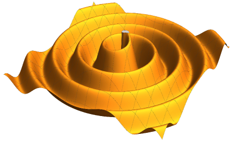
The solution (16 z = 0 𝑧 0 z=0 ρ = 0 𝜌 0 \rho=0 z → ± ∞ → 𝑧 plus-or-minus z\to\pm\infty ( z = 0 ) ∩ ( x 0 = 0 ) 𝑧 0 superscript 𝑥 0 0 (z=0)\cap(x^{0}=0) 16 m = 1 𝑚 1 m=1 ω = λ = 1 𝜔 𝜆 1 \omega=\lambda=1 1
Figure 1: Section ( z = 0 ) ∩ ( x 0 = 0 ) 𝑧 0 superscript 𝑥 0 0 (z=0)\cap(x^{0}=0) 16 m = 1 𝑚 1 m=1 ω = λ = 1 𝜔 𝜆 1 \omega=\lambda=1
In view of the equation of motion (12 ∼ Γ 00 i \mathchoice{{\hbox to0.0pt{\hskip 0.43057pt\raisebox{6.45831pt}{${\scriptstyle\sim}$}\hss}}\Gamma}{{\hbox to0.0pt{\hskip 0.43057pt\raisebox{6.45831pt}{${\scriptstyle\sim}$}\hss}}\Gamma}{{\hbox to0.0pt{\raisebox{4.95134pt}{${\scriptscriptstyle\sim}$}\hss}}\Gamma}{}{}^{i}_{00} 14 Φ Φ \Phi
⋅ v 2 ρ = ∼ Γ 00 1 ⟹ ⋅ v = ρ ∼ Γ 00 1 , ∼ Γ ⩾ 00 1 0 , \displaystyle\frac{\mathchoice{{\hbox to0.0pt{\hskip 1.29167pt\raisebox{-0.43057pt}{${\boldsymbol{\cdot}}$}\hss}}v}{{\hbox to0.0pt{\hskip 1.29167pt\raisebox{-0.43057pt}{${\boldsymbol{\cdot}}$}\hss}}v}{{\hbox to0.0pt{\hskip 0.86108pt\raisebox{-0.21529pt}{${\scriptstyle\boldsymbol{\cdot}}$}\hss}}v}{}{}^{2}}{\rho}=\mathchoice{{\hbox to0.0pt{\hskip 0.43057pt\raisebox{6.45831pt}{${\scriptstyle\sim}$}\hss}}\Gamma}{{\hbox to0.0pt{\hskip 0.43057pt\raisebox{6.45831pt}{${\scriptstyle\sim}$}\hss}}\Gamma}{{\hbox to0.0pt{\raisebox{4.95134pt}{${\scriptscriptstyle\sim}$}\hss}}\Gamma}{}{}^{1}_{00}\quad\Longrightarrow\quad\mathchoice{{\hbox to0.0pt{\hskip 1.29167pt\raisebox{-0.43057pt}{${\boldsymbol{\cdot}}$}\hss}}v}{{\hbox to0.0pt{\hskip 1.29167pt\raisebox{-0.43057pt}{${\boldsymbol{\cdot}}$}\hss}}v}{{\hbox to0.0pt{\hskip 0.86108pt\raisebox{-0.21529pt}{${\scriptstyle\boldsymbol{\cdot}}$}\hss}}v}{}{}=\sqrt{\rho\,\mathchoice{{\hbox to0.0pt{\hskip 0.43057pt\raisebox{6.45831pt}{${\scriptstyle\sim}$}\hss}}\Gamma}{{\hbox to0.0pt{\hskip 0.43057pt\raisebox{6.45831pt}{${\scriptstyle\sim}$}\hss}}\Gamma}{{\hbox to0.0pt{\raisebox{4.95134pt}{${\scriptscriptstyle\sim}$}\hss}}\Gamma}{}{}^{1}_{00}}\;,\quad\mathchoice{{\hbox to0.0pt{\hskip 0.43057pt\raisebox{6.45831pt}{${\scriptstyle\sim}$}\hss}}\Gamma}{{\hbox to0.0pt{\hskip 0.43057pt\raisebox{6.45831pt}{${\scriptstyle\sim}$}\hss}}\Gamma}{{\hbox to0.0pt{\raisebox{4.95134pt}{${\scriptscriptstyle\sim}$}\hss}}\Gamma}{}{}^{1}_{00}\geqslant 0\;, (17a)
∼ Γ ≈ 00 1 ( ∂ ∼ 𝔪 ˇ 01 ∂ x 0 − 1 2 ∂ ∼ 𝔪 ˇ 00 ∂ ρ ) ≈ 4 π χ 2 ( ∂ 𝒫 ¯ 1 ∂ x 0 − 1 2 ∂ ℰ ¯ ∂ ρ ) . \displaystyle\mathchoice{{\hbox to0.0pt{\hskip 0.43057pt\raisebox{6.45831pt}{${\scriptstyle\sim}$}\hss}}\Gamma}{{\hbox to0.0pt{\hskip 0.43057pt\raisebox{6.45831pt}{${\scriptstyle\sim}$}\hss}}\Gamma}{{\hbox to0.0pt{\raisebox{4.95134pt}{${\scriptscriptstyle\sim}$}\hss}}\Gamma}{}{}^{1}_{00}\approx\left(\frac{\partial\check{\mathchoice{{\hbox to0.0pt{\hskip 0.86108pt\raisebox{4.30554pt}{${\scriptstyle\sim}$}\hss}}\mathfrak{m}}{{\hbox to0.0pt{\hskip 0.86108pt\raisebox{4.30554pt}{${\scriptstyle\sim}$}\hss}}\mathfrak{m}}{{\hbox to0.0pt{\hskip 0.21529pt\raisebox{2.84166pt}{${\scriptscriptstyle\sim}$}\hss}}\mathfrak{m}}{}{}}_{01}}{\partial x^{0}}-\frac{1}{2}\,\frac{\partial\check{\mathchoice{{\hbox to0.0pt{\hskip 0.86108pt\raisebox{4.30554pt}{${\scriptstyle\sim}$}\hss}}\mathfrak{m}}{{\hbox to0.0pt{\hskip 0.86108pt\raisebox{4.30554pt}{${\scriptstyle\sim}$}\hss}}\mathfrak{m}}{{\hbox to0.0pt{\hskip 0.21529pt\raisebox{2.84166pt}{${\scriptscriptstyle\sim}$}\hss}}\mathfrak{m}}{}{}}_{00}}{\partial\rho}\right)\approx 4\pi\,\chi^{2}\left(\frac{\partial\bar{\mathcal{P}}^{1}}{\partial x^{0}}-\frac{1}{2}\,\frac{\partial\bar{\mathcal{E}}}{\partial\rho}\right)\;. (17b)
Here for ∼ Γ < 00 1 0 \mathchoice{{\hbox to0.0pt{\hskip 0.43057pt\raisebox{6.45831pt}{${\scriptstyle\sim}$}\hss}}\Gamma}{{\hbox to0.0pt{\hskip 0.43057pt\raisebox{6.45831pt}{${\scriptstyle\sim}$}\hss}}\Gamma}{{\hbox to0.0pt{\raisebox{4.95134pt}{${\scriptscriptstyle\sim}$}\hss}}\Gamma}{}{}^{1}_{00}<0
The orbital velocity (17a 16 ( z = 0 ) ∩ ( φ = 0 ) ∩ ( x 0 = 0 ) 𝑧 0 𝜑 0 superscript 𝑥 0 0 (z=0)\cap(\varphi=0)\cap(x^{0}=0) m = 1 𝑚 1 m=1 ω = λ = 1 𝜔 𝜆 1 \omega=\lambda=1 3 ( z = 0 ) ∩ ( x 0 = 0 ) 𝑧 0 superscript 𝑥 0 0 (z=0)\cap(x^{0}=0) m = 1 𝑚 1 m=1 ω = λ = 1 𝜔 𝜆 1 \omega=\lambda=1 3
As can be seen on Fig. 3 3
It should be noted that for the considered simple asymptotics of galaxy soliton (16 2 m 2 𝑚 2\,m m 𝑚 m
Here we have considered only one possible asymptotics of a galactic soliton which coincides with experimental data. But, apparently, for any real galaxy
we can discover the appropriate asymptotic solution of the space-time film equation which gives an observable distribution of star density and orbital velocities.
This will mean that for this galaxy we have obtained the asymptotics of the appropriate galactic soliton.