Quantification of parametric uncertainties
induced by irregular soil loading in orchard
tower sprayer nonlinear dynamics

Abstract

This paper deals with the nonlinear stochastic dynamics of an orchard tower sprayer subjected to random excitations due to soil irregularities. A consistent stochastic model of uncertainties is constructed to describe random loadings and to predict variabilities in mechanical system response. The dynamics is addressed in time and frequency domains. Monte Carlo method is employed to compute the propagation of uncertainties through the stochastic model. Numerical simulations reveals a very rich dynamics, which is able to produce chaos. This numerical study also indicates that lateral vibrations follow a direct energy cascade law. A probabilistic analysis reveals the possibility of large lateral vibrations during the equipment operation.

1 Introduction

The proliferation of pests in agricultural industry can be harmful to consumers and producers, since it can cause problems such as a reduction in the products quality, partial/total loss of the plantation, etc. Thus, the process of agricultural spraying for pest control is of great importance in orchards, vegetable gardens, etc. In general, the spraying of orchards is done with the aid of an equipment called tower sprayer, that consists of a reservoir and several fans mounted on an articulated tower, which is supported by a vehicle suspension [1]. Due to soil irregularities this equipment is subjected to loads of random nature, which may hamper the fluid spraying proper dispersion.

Primary studies on this topic are presented in [1, 2, 3], using a mathematical model that considers an inverted pendulum mounted on a moving base to emulate the equipment. These works perform deterministic analyzes to investigate the influence of certain parameters (stiffness, torsional damping, etc) in the model response. In addition, references [2] and [3] present a detailed study of the associated linear dynamics. In all cases, the observed behavior is physically reasonable, but also the analyzes are limited to simple situations, once the model does not take into account the system dynamics underlying uncertainties. In fact, system parameters have uncertainties due to a series of factors such as variabilities intrinsic to the manufacturing process, materials and geometric imperfections, etc [4, 5]. Taking such uncertainties into account is essential for making robust predictions, but also, it has been becoming a common practice in engineering [6, 7, 8, 9, 10].

In this sense, this paper aims to construct a consistent stochastic model to describe the nonlinear dynamics of an orchard tower sprayer, taking parametric uncertainties into account. In a first analysis, the authors concentrate their efforts in tires excitation uncertainties, induced by soil irregularities, once these loads are extremely complex and have great influence in the system dynamics. For this purpose, it is more realistic to describe the system dynamics by means of a probabilistic model of uncertainties, since in this type of approach uncertainties are naturally characterized [4]. Some initiatives in this direction were presented by the authors in two conference papers [11, 12], where a harmonic random process was used to emulate the aleatory loadings. But now, they intend to construct the random excitations using Karhunen-Loève (KL) decomposition, seeking a better characterization of the loads. This work also intends to deeply investigate in depth the effects of random excitation in the tower sprayer response, and compute the probability of undesirable operating events, such as large lateral vibrations.

The rest of this paper is organized as follows. In section 2, it is presented a deterministic model to describe the sprayer nonlinear dynamics. A stochastic model to to take into account the uncertainties associated with the soil induced loading is shown in section 3. The results of the numerical experiments conducted in this work are presented and discussed in section 4. Finally, in section 5, the main conclusions are highlighted, and some paths for future works are indicated.

2 Deterministic modeling

2.1 Physical system definition

The mechanical system of interest here is the tower sprayer schematically represented in Figure 1. It consists of a reservoir tank, used to store a spraying fluid, which is mounted onto a vehicular suspension. In this suspension, there is a support tower where sixteen fans are arranged in columns, eight on the right and eight pointing to left. These fans are used to pulverize an orchard. As this equipment moves through a rough terrain, vertical and horizontal vibrations may be observed.

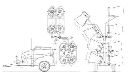
Figure 1: Schematic representation of the tower sprayer. Adapted from [2] and courtesy of Máquinas Agrícolas Jacto S/A.

2.2 Physical system parameterization

For modeling purposes the orchard sprayer tower is considered as the multibody system illustrated in Figure 2, such as proposed by [1, 2]. Suspension chassis and reservoir tank are emulated by a rigid trailer with mass $\displaystyle m_{1}$. The vertical tower and funs are modeled by an inverted rigid pendulum of mass $\displaystyle m_{2}$. Their moments of inertia, with respect to their center of gravity, are respectively denoted by $\displaystyle I_{1}$ and $\displaystyle I_{2}$. The point of articulation between the trailer and tower, denoted by $\displaystyle P$, has torsional stiffness $\displaystyle k_{T}$ and damping torsional coefficient $\displaystyle c_{T}$. Its distance to the trailer center of gravity is $\displaystyle L_{1}$ and the pendulum arm length is dubbed $\displaystyle L_{2}$. The left wheel of the vehicle suspension, located at a distance $\displaystyle B_{1}$ from trailer center line, is represented by a pair spring/damper with constants $\displaystyle k_{1}$ and $\displaystyle c_{1}$, respectively, and it is subject to a vertical displacement $\displaystyle y_{e1}$. Similarly, the right wheel is represented by a pair spring/damper characterized by $\displaystyle k_{2}$ and $\displaystyle c_{2}$, it is $\displaystyle B_{2}$ away from the trailer center line, and it displaces vertically $\displaystyle y_{e2}$. For simplicity, the sprayer translational velocity is supposed to be a constant v. The acceleration of gravity is denoted by $\displaystyle g$.

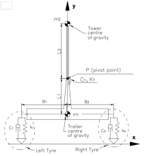
Figure 2: Schematic representation of the mechanical-mathematical model for the tower sprayer: an inverted pendulum mounted on a rigid trailer. (a) Static equilibrium configuration; (b) Off equilibrium configuration. Adapted from [2].

Introducing the inertial frame of reference $\displaystyle XY$, the horizontal and vertical displacements of the trailer center of mass are respectively measured by $\displaystyle x_{1}$ and $\displaystyle y_{1}$, while its rotation is computed by $\displaystyle\phi_{1}$. The horizontal and vertical displacements of the tower center of mass are given by $\displaystyle x_{2}$ and $\displaystyle y_{2}$, respectively, and its rotation with respect to the trailer is denoted by $\displaystyle\phi_{2}$.

As the trailer horizontal movement is limited by the pair of tires, one has $\displaystyle x_{1}=0$. It can also be deduced from the geometry of Figure 2 that

$$x_{2}=-L_{1}\,\sin\phi_{1}-L_{2}\,\sin\phi_{2},$$ (1)

and

$$y_{2}=y_{1}+L_{1}\,\cos\phi_{1}+L_{2}\,\cos\phi_{2}.$$ (2)

Therefore, this model has degrees of freedom: $\displaystyle y_{1}$, $\displaystyle\phi_{1}$ and $\displaystyle\phi_{2}$. The main quantity of interest (QoI) in the study of this dynamics is the time function $\displaystyle x_{2}$.

2.3 Lagrangian formalism

Euler-Lagrange equations are employed to obtain the system dynamics

$$\mathinner{\dfrac{\partial{}}{\partial{t}}}\left(\mathinner{\dfrac{\partial{}\mathcal{T}}{\partial{\dot{q}}}}\right)-\mathinner{\dfrac{\partial{}\mathcal{T}}{\partial{q}}}+\mathinner{\dfrac{\partial{}\mathcal{V}}{\partial{q}}}+\mathinner{\dfrac{\partial{}\mathcal{D}}{\partial{\dot{q}}}}=0,\leavevmode\nobreak\ \leavevmode\nobreak\ \leavevmode\nobreak\ q=\{y_{1},\phi_{1},\phi_{2}\},$$ (3)

where the upper dot is an abbreviation for time derivative, and the functionals of kinetic energy, potential energy and dissipation are, respectively, given by

$$\mathcal{T}=\frac{1}{2}m_{1}\,\dot{y}_{1}+\frac{1}{2}m_{2}\left(\dot{x}_{2}+\dot{y}_{2}\right)+\frac{1}{2}I_{1}\dot{\phi}_{1}+\frac{1}{2}I_{2}\dot{\phi}_{2},$$ (4)

$$\begin{split}\mathcal{V}=m_{1}\,g\,y_{1}+m_{2}\,g\,y_{2}+\frac{1}{2}k_{1}\left(y_{1}-B_{1}\,\sin{\phi_{1}}-y_{e1}\right)^{2}+\\ \frac{1}{2}k_{2}\left(y_{1}+B_{2}\,\sin{\phi_{1}}-y_{e2}\right)^{2}+\frac{1}{2}k_{T}\left(\phi_{2}-\phi_{1}\right)^{2},\end{split}$$ (5)

and

$$\begin{split}\mathcal{D}=\frac{1}{2}c_{1}\left(\dot{y}_{1}-B_{1}\,\dot{\phi}_{1}\,\cos{\phi_{1}}-y_{e1}\right)^{2}+\\ \frac{1}{2}c_{2}\left(\dot{y}_{1}+B_{2}\,\dot{\phi}_{1}\,\cos{\phi_{1}}-y_{e1}\right)^{2}+\frac{1}{2}c_{T}\left(\dot{\phi}_{2}-\dot{\phi}_{1}\right)^{2}.\end{split}$$ (6)

After the calculation, the following set of nonlinear ordinary differential equations is obtained

(19)

where $\displaystyle\mathbf{M}$, $\displaystyle\mathbf{N}$, $\displaystyle\mathbf{C}$ and $\displaystyle\mathbf{N}$ are $\displaystyle 3\times 3$ (configuration dependent) real matrices, respectively, defined by

(23)

$$\displaystyle\mathbf{N}=\left[\begin{array}[]{ccc}0&-m_{2}\,L_{1}\,\cos\phi_{1}&-m_{2}\,L_{2}\,\cos\phi_{2}\\ 0&0&-m_{2}\,L_{1}\,L_{2}\,\sin\left(\phi_{2}-\phi_{1}\right)\\ 0&-m_{2}\,L_{1}\,L_{2}\,\sin\left(\phi_{2}-\phi_{1}\right)&0\\ \end{array}\right],$$ (27)

$$\displaystyle\mathbf{C}=\left[\begin{array}[]{ccc}c_{1}+c_{2}&(c_{2}\,B_{2}-c_{1}\,B_{1})\cos\phi_{1}&0\\ (c_{2}\,B_{2}-c_{1}\,B1)\cos\phi_{1}&c_{T}+(c_{1}\,B^{2}_{1}+c_{2}\,B^{2}_{2})\cos^{2}\phi_{1}&-c_{T}\\ 0&-c_{T}&c_{T}\\ \end{array}\right],$$ (31)

and

$$\displaystyle\mathbf{K}=\left[\begin{array}[]{ccc}k_{1}+k_{2}&0&0\\ (k_{2}\,B_{2}-k_{1}\,B1)\cos\phi_{1}&k_{T}&-k_{T}\\ 0&-k_{T}&k_{T}\\ \end{array}\right],$$ (35)

and $\displaystyle\mathbf{g}$ and $\displaystyle\mathbf{h}$ are (configuration dependent) vectors in $\displaystyle\mathbb{R}^{3}$, respectively, defined by

$$\displaystyle\mathbf{g}=\left(\begin{array}[]{c}(k_{2}\,B_{2}-k_{1}\,B_{1})\sin\phi_{1}+(m_{1}+m_{2})g\\ (k_{1}\,B_{1}^{2}+k_{2}\,B_{2}^{2})\sin\phi_{1}\,\cos\phi_{1}-m_{2}\,g\,L_{1}\,\sin\phi_{1}\\ -m_{2}\,g\,L_{2}\,\sin\phi_{2}\\ \end{array}\right),$$ (39)

and

(43)

The deduction of Eq.(19) can be seen in detail in [2], which also obtain this set of equations through a Newtonian formulation.

2.4 Static equilibrium configuration

The static equilibrium configuration for the tower sprayer, illustrated in Figure 2(a), and defined by

$$y_{1}(0)=-\frac{(m_{1}+m_{2})}{k_{1}+k_{2}}\,g,\qquad\phi_{1}(0)=0,\qquad\phi_{2}(0)=0,$$ (44)

and

$$\dot{y}_{1}(0)=0,\qquad\dot{\phi}_{1}(0)=0,\qquad\dot{\phi}_{2}(0)=0.$$ (45)

is assumed as the initial state of the system. This is a stable equilibrium, where the system presents neither velocity nor any rotation, but has a negative vertical displacement with respect to the level of reference.

2.5 Nonlinear initial value problem

By means of the generalized displacement $\displaystyle\mathbf{q}\mathrel{\mathop{\mathchar 58\relax}}t\in\mathbb{R}\mapsto\mathbf{q}(t)\in\mathbb{R}^{6}$, the initial displacement vector $\displaystyle\mathbf{q}_{0}\in\mathbb{R}^{6}$, and the nonlinear mapping $\displaystyle\mathbf{f}\mathrel{\mathop{\mathchar 58\relax}}\left(t,\mathbf{q}(t)\right)\in\mathbb{R}\times\mathbb{R}^{6}\mapsto\mathbf{f}\left(\mathbf{q}(t)\right)\in\mathbb{R}^{6}$, where

$$\displaystyle\mathbf{q}(t)=\left(\begin{array}[]{c}y_{1}(t)\\ \phi_{1}(t)\\ \phi_{2}(t)\\ \dot{y}_{1}(t)\\ \dot{\phi}_{1}(t)\\ \dot{\phi}_{2}(t)\\ \end{array}\right),\qquad\mathbf{q}_{0}=\left(\begin{array}[]{c}y_{1}(0)\\ \phi_{1}(0)\\ \phi_{2}(0)\\ \dot{y}_{1}(0)\\ \dot{\phi}_{1}(0)\\ \dot{\phi}_{2}(0)\\ \end{array}\right),$$ (58)

and

(72)

it is possible write the dynamical system of Eqs.(19), (44) and (45) as

$$\mathbf{\dot{q}}(t)=\mathbf{f}\left(\mathbf{q}(t)\right),\qquad\mathbf{q}(0)=\mathbf{q}_{0},$$ (73)

a nonlinear initial value problem that is integrated using Runge-Kutta-Fehlberg method (RKF45) [13, 14].

3 Stochastic modeling

3.1 Aleatory nature of a tire displacement

Typical paths followed by sprayer tower during its operation are illustrated in Figure 3, which shows tires vertical displacement as function of the traveled distance. Note that sprayer tires undergo irregular displacements, which resembles a random signal not a smooth function. In this way, it is better to describe the irregular form of tires displacement, and therefore, the sprayer tower dynamics, with a stochastic dynamic model.

(a) left tire path

(b) right tire path

Figure 3: Illustration of typical paths followed by sprayer tower tires during operation. Adapted from [1].

3.2 Probabilistic framework

In this work the mechanical system stochastic dynamics is described through a parametric probabilistic approach [4, 5], which uses the probability space $\displaystyle(\SS,\mathbb{\Sigma},\mathbb{P})$, being $\displaystyle\SS$ the sample space, $\displaystyle\mathbb{\Sigma}$ a $\displaystyle\sigma$-field over $\displaystyle\SS$, and $\displaystyle\mathbb{P}\mathrel{\mathop{\mathchar 58\relax}}\mathbb{\Sigma}\to[0,1]$ the probability measure. Within this framework, the mathematical expectation operator is defined by

$$E\left\{\mathbb{y}\right\}=\int_{\mathbb{R}}y\,dF_{\tiny{\mathbb{y}}}(y)\,,$$ (74)

where $\displaystyle\mathbb{y}$ is a real-valued random variable defined in $\displaystyle(\SS,\mathbb{\Sigma},\mathbb{P})$, with probability distribution $\displaystyle F_{\tiny{\mathbb{y}}}(y)$. With the aid of Eq.(74) it is possible to define statistics of $\displaystyle\mathbb{y}$ such as mean value $\displaystyle\mu_{\mathbb{y}}=E\left\{\mathbb{y}\right\}$, variance $\displaystyle\sigma^{2}_{\mathbb{y}}=E\left\{\left(\mathbb{y}-\mu_{\mathbb{y}}\right)^{2}\right\}$, and standard deviation $\displaystyle\sigma_{\mathbb{y}}=\sqrt{\sigma^{2}_{\mathbb{y}}}$. Note that for random processes, which are “time-dependent random variables”, these statistics present time dependence. Furthermore, the covariance function of random process $\displaystyle\left\{\mathbb{y}(t),t\in\mathbb{R}\right\}$, at time instants $\displaystyle t_{1}$ and $\displaystyle t_{2}$, is defined by $\displaystyle C_{\mathbb{y}}(t_{1},t_{2})=E\left\{\left(\mathbb{y}(t_{1})-\mu_{\mathbb{y}}(t_{1})\right)\left(\mathbb{y}(t_{2})-\mu_{\mathbb{y}}(t_{2})\right)\right\}$.

3.3 Tire displacement modeling

The tire displacements have aleatory nature and present time dependence, so that they can be described by square-integrable random processes $\displaystyle\left\{\mathbb{y}_{e1}(t),t\in\mathbb{R}\right\}$ and $\displaystyle\left\{\mathbb{y}_{e2}(t),t\in\mathbb{R}\right\}$. Accordingly, the trajectories illustrated in Figure  3 can be thought as sample paths associated to these processes.

The dynamic behavior of one tire certainly influences the way other tire behaves, i.e., there is some dependence between the two random processes. However, for lack of better knowledge about the correlation between $\displaystyle\mathbb{y}_{e1}(t)$ and $\displaystyle\mathbb{y}_{e2}(t)$, these random processes are assumed to be independent. For convenience, they are also assumed to be stationary, which implies that the means values $\displaystyle\mu_{\mathbb{y}_{e1}}$ and $\displaystyle\mu_{\mathbb{y}_{e2}}$ are constant, as well as the standard deviations $\displaystyle\sigma_{\mathbb{y}_{e1}}$ and $\displaystyle\sigma_{\mathbb{y}_{e2}}$.

Once the tire displacement at certain instant of time has little influence on the value of this kinematic parameter at a distant time, it is also reasonable to assume that covariance functions of these processes present exponentially decaying behavior, i.e.,

$$C_{\mathbb{y}_{e1}}(t_{1},t_{2})=C_{\mathbb{y}_{e2}}(t_{1},t_{2})=\exp{\left(-\frac{t_{2}-t_{1}}{a_{corr}/v}\right)}\,,$$ (75)

where $\displaystyle v$ is the translational velocity of the sprayer tower (supposed as constant) and $\displaystyle a_{corr}$ is a correlation length for the processes $\displaystyle\mathbb{y}_{e1}(t)$ and $\displaystyle\mathbb{y}_{e2}(t)$.

3.4 Random processes representation

From the theoretical point of view, random processes $\displaystyle\mathbb{y}_{e1}(t)$ and $\displaystyle\mathbb{y}_{e2}(t)$ are well defined with the information given in section 3.3. However, for computational implementation purposes, it is necessary to represent these random processes (infinite-dimensional objects) in terms of a finite number of random variables [15].

This task can be efficiently done through the truncation of Karhunen-Loève (KL) decomposition [16, 15], which is a powerful tool to represent random fields/processes [17, 18, 19, 20, 21, 22, 23].

KL expansion of $\displaystyle\left\{\mathbb{y}(t),t\in\mathbb{R}\right\}$ writes as

$$\mathbb{y}(t)=\mu_{\mathbb{y}}(t)+\sum_{n=1}^{+\infty}\sqrt{\lambda_{n}}\,\varphi_{n}(t)\,\mathbb{Y}_{n},$$ (76)

where the pairs $\displaystyle\left(\lambda_{n},\varphi_{n}\right)$ are solution of Fredholm integral equation

$$\int_{\mathbb{R}}C_{{y}(t)}(t,s)\,\varphi_{n}(s)\,ds=\lambda_{n}\,\varphi_{n}(t),\qquad t\in\mathbb{R},$$ (77)

and $\displaystyle\left\{\mathbb{Y}_{n}\right\}_{n=1}^{+\infty}$ is a family of zero-mean mutually uncorrelated random variables, i.e.,

$$\mu_{\mathbb{Y}_{n}}=0,\qquad\mbox{and}\qquad E\left\{\mathbb{Y}_{n}\mathbb{Y}_{m}\right\}=\delta_{mn}.$$ (78)

The approximation is obtained after the truncation of Eq.(76), i.e.,

$$\mathbb{y}(t)\approx\mu_{\mathbb{y}}(t)+\sum_{n=1}^{N_{KL}}\sqrt{\lambda_{n}}\,\varphi_{n}(t)\,\mathbb{Y}_{n},$$ (79)

where the integer $\displaystyle N_{KL}$ is chosen such that

$$\frac{\sum_{n=1}^{N_{KL}}\lambda_{n}}{\sum_{n=1}^{+\infty}\lambda_{n}}\geq\tau,$$ (80)

with $\displaystyle\tau=99.9\%$, such as suggested by [24].

The simulations reported here use a family of zero-mean uncorrelated Gaussian random variables for $\displaystyle\left\{\mathbb{Y}_{n}\right\}_{n=1}^{N_{KL}}$, which generate a stochastic process which sample paths can be seen in Figure 4. From the qualitative point of view these realizations of the random process emulate the tracks shown in Figure 3.

(a) $\displaystyle\mathbb{y}_{e1}$ path (left tire)

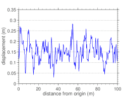
(b) $\displaystyle\mathbb{y}_{e2}$ path (right tire)

Figure 4: Illustration of sample paths associated to the stationary square-integrable random process generated by the truncated KL decomposition, with $\displaystyle v=12$ km/h, $\displaystyle a_{corr}=1$ m, $\displaystyle\sigma_{\mathbb{y}}=0.175$ m and $\displaystyle\mu_{\mathbb{y}}=0.5$ m.

3.5 Random nonlinear dynamical system

Due to the randomness of $\displaystyle\mathbb{y}_{e1}$ and $\displaystyle\mathbb{y}_{e2}$ the mechanical system response becomes aleatory, described by the real-valued random processes $\displaystyle\mathbb{y}_{1}$, $\displaystyle\bbphi_{1}$ and $\displaystyle\bbphi_{2}$.

Therefore, the mechanical system dynamic behavior evolves (almost sure) according to the random nonlinear dynamical system defined by

(93)

where the real-valued random matrices/vectors $\displaystyle\mathbf{\mathbb{M}}$, $\displaystyle\mathbf{\mathbb{N}}$, $\displaystyle\mathbf{\mathbb{C}}$, $\displaystyle\mathbf{\mathbb{K}}$, $\displaystyle\mathbb{g}$ and $\displaystyle\mathbb{h}$ are stochastic versions of the matrices/vectors $\displaystyle\mathbf{M}$, $\displaystyle\mathbf{N}$, $\displaystyle\mathbf{C}$, $\displaystyle\mathbf{K}$, $\displaystyle\mathbf{g}$ and $\displaystyle\mathbf{h}$.

3.6 Monte Carlo method: the stochastic solver

Monte Carlo (MC) method [25, 26] is employed to compute the propagation of uncertainties of the random parameters through the nonlinear dynamics defined by Eq.(93). The convergence of MC simulations is evaluated through the map $\displaystyle\texttt{conv}\mathrel{\mathop{\mathchar 58\relax}}n_{s}\in\mathbb{N}\mapsto\texttt{conv}(n_{s})\in\mathbb{R}$, where $\displaystyle n_{s}$ is the number of MC realizations, $\displaystyle\theta_{n}$ denotes the n-the MC realization, $\displaystyle[t_{0},t_{f}]$ is the time interval of analysis, and

$$\texttt{conv}(n_{s})=\left(\frac{1}{n_{s}}\sum_{n=1}^{n_{s}}\int_{t=t_{0}}^{t_{f}}\left(\mathbb{y}_{1}(t,\theta_{n})^{2}+\bbphi_{1}(t,\theta_{n})^{2}+\bbphi_{2}(t,\theta_{n})^{2}\right)\,dt\right)^{1/2}.$$ (94)

This metric allows one to evaluate the convergence of the approximation $\displaystyle\left(\mathbb{y}_{1}(t,\theta_{n}),\bbphi_{1}(t,\theta_{n}),\bbphi_{2}(t,\theta_{n})\right)^{\scriptscriptstyle T}$ in the mean-square sense. See [27] for further details.

4 Numerical experiments

The physical parameters adopted in the simulation of the mechanical system are presented in Table 1. They correspond to the nominal parameters of an sprayer tower model Arbus Multisprayer 4000, illustrated in Figure 1, whose values can be seen in [1].

Table 1: Physical parameters for the mechanical system used in the simulations.

parameter	value	unit
$\displaystyle m_{1}$	$\displaystyle 6500$	kg
$\displaystyle m_{2}$	$\displaystyle 800$	kg
$\displaystyle L_{1}$	$\displaystyle 0.2$	m
$\displaystyle L_{2}$	$\displaystyle 2.4$	m
$\displaystyle I_{1}$	$\displaystyle 6850$	kg   m2
$\displaystyle I_{2}$	$\displaystyle 6250$	kg   m2
$\displaystyle k_{1}$	$\displaystyle 465\times 10^{3}$	N/m
$\displaystyle k_{2}$	$\displaystyle 465\times 10^{3}$	N/m
$\displaystyle c_{1}$	$\displaystyle 5.6\times 10^{3}$	N/m/s
$\displaystyle c_{2}$	$\displaystyle 5.6\times 10^{3}$	N/m/s
$\displaystyle B_{1}$	$\displaystyle 0.85$	m
$\displaystyle B_{2}$	$\displaystyle 0.85$	m
$\displaystyle k_{T}$	$\displaystyle 100\times 10^{3}$	N/rad
$\displaystyle c_{T}$	$\displaystyle\leavevmode\nobreak\ 40\times 10^{3}$	N m/rad/s

Moreover, the parameters which define the random loadings can be seen in Table 2. They are obtained via educated judgment, trial and error, always checking if the behavior of the tower sprayer was in agreement with the intuition of the authors about this physical system. In fact, it is reasonable to assume that the radius of mutual influence (correlation) between soil irregularities has the same order of magnitude as the sprayer tower tires diameters. Once each tire has a diameter of the order of magnitude of $\displaystyle 1\,m$, it is assumed that $\displaystyle a_{corr}=1\,m$. The displacements $\displaystyle\mathbb{y}_{e1}(t)$ and $\displaystyle\mathbb{y}_{e2}(t)$ correspond to vertical translations of the tires centroids, which on a soil without irregularities will be approximately $\displaystyle 0.5$ m above the ground (half of the tire diameter). Therefore, $\displaystyle\mu_{y}=0.5$ m is adopted. The choice of standard deviation values corresponds to a dispersion level of 35%, which provides stringent soil-irregularities induced loadings. The latter is necessary to investigate severe conditions of lateral (horizontal) vibrations.

Table 2: Parameters that define the stochastic loadings.

parameter	value	unit
$\displaystyle N_{KL}$	$\displaystyle 403$	—
$\displaystyle a_{corr}$	$\displaystyle 1$	m
$\displaystyle\sigma_{y_{e1}}$	$\displaystyle 0.175$	m
$\displaystyle\sigma_{y_{e2}}$	$\displaystyle 0.175$	m
$\displaystyle\mu_{y_{e1}}$	$\displaystyle 0.5$	m
$\displaystyle\mu_{y_{e2}}$	$\displaystyle 0.5$	m
$\displaystyle v$	$\displaystyle 12$	km/h

A representative band of frequencies for the present problem is given by $\displaystyle\mathcal{B}=[0,5]$ Hz, once the sprayer tower operates on the low frequency range. Thus, the evolution of the nonlinear dynamic system is addressed using a nominal time step $\displaystyle\Delta t=1\times 10^{-3}$ s, which is refined whenever necessary to capture the nonlinear effects.

4.1 Nonlinear dynamics animation

In a first moment, the nonlinear dynamics is explored in the temporal window defined by $\displaystyle[t_{0},t_{f}]=[0,30]$ s. This time-interval corresponds to a traveled path of $\displaystyle 100$ m, such as those shown in Figure 3.

An animation of the mechanical dynamic system, for different instants of time in $\displaystyle[t_{0},t_{f}]$, is shown in Figure 5. In this animation the mechanical system is supported on the ground (gray shaded region bounded by a black thick line), the tires are represented by black vertical rectangles, the red lines correspond to the trailer and the tower is illustrated as a thicker blue line. The video animation is available in Supplementary Material 1 [28].

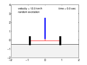
(a) $\displaystyle t=0$s

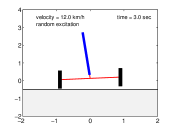
(b) $\displaystyle t=3$ s

(c) $\displaystyle t=7$ s

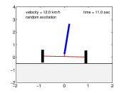
(d) $\displaystyle t=11$ s

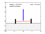
(e) $\displaystyle t=15$ s

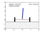
(f) $\displaystyle t=18$ s

(g) $\displaystyle t=22$ s

(h) $\displaystyle t=26$ s

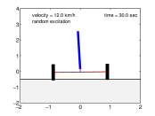
(i) $\displaystyle t=30$ s

Figure 5: Animation of the mechanical system at different instants of time.

4.2 Time domain analysis

The time series corresponding to the trailer/tower vertical dynamics $\displaystyle y_{1}$/$\displaystyle y_{2}$ can be seen in Figure 6, while the corresponding phase space trajectory projections (in $\displaystyle\mathbb{R}^{3}$ and $\displaystyle\mathbb{R}^{2}$) are presented in Figure 7.

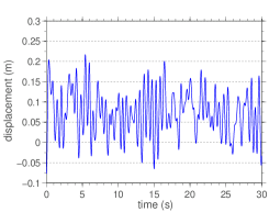
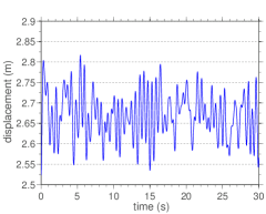
Figure 6: Time series of vertical nonlinear dynamics. (a) trailer displacement $\displaystyle y_{1}$; (b) tower displacement $\displaystyle y_{2}$; (b) difference between $\displaystyle y_{2}$ and $\displaystyle y_{1}$.

It may be noted from Figure 6 that both $\displaystyle y_{1}$ and $\displaystyle y_{2}$ have irregular oscillatory behavior, which are quite similar. The difference between $\displaystyle y_{2}$ and $\displaystyle y_{1}$ is very small, and can be seen in Figure 6. The strong correlation between the two time series is visually noticeable. The trajectories projections shown in Figure 7 corroborate the previous statement.

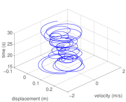
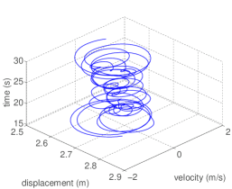
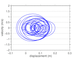
Figure 7: Projections of vertical dynamics phase space trajectories. (a) $\displaystyle y_{1}$ atractor in $\displaystyle\mathbb{R}^{3}$; (b) $\displaystyle y_{2}$ atractor in $\displaystyle\mathbb{R}^{3}$; (c) $\displaystyle y_{1}$ atractor in $\displaystyle\mathbb{R}^{2}$; (d) $\displaystyle y_{2}$ atractor in $\displaystyle\mathbb{R}^{2}$.

The time series corresponding to the trailer/tower rotational dynamics $\displaystyle\phi_{1}$/$\displaystyle\phi_{2}$ is available in Figure 8, and the respective phase space trajectories projections are shown in Figure 9.

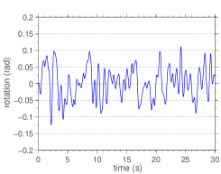
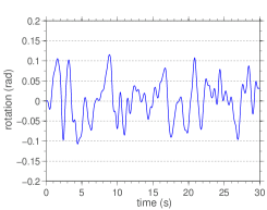
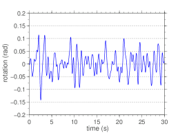
Figure 8: Time series of rotational nonlinear dynamics. (a) trailer rotation $\displaystyle\phi_{1}$; (b) tower rotation $\displaystyle\phi_{2}$; (c) difference between $\displaystyle\phi_{2}$ and $\displaystyle\phi_{1}$.

Observe that in Figure 8 the correlation between the time series is still strong, but there is a kind of filter effect, which can also be noticed in the projected trajectories in Figure 9. Such trajectories seem to accumulate into a strange attractor, which justifies the irregular and intermittent appearance of the corresponding time series. However, unlike for $\displaystyle y_{1}$ and $\displaystyle y_{2}$, now the difference between the two time series is not negligible. This significant difference between the rotations is responsible for nonlinear effects of inertia and damping. This is clear when looking at the matrices of Eqs.(23) and (27), which have trigonometric terms that depend on $\displaystyle\phi_{2}-\phi_{1}$.

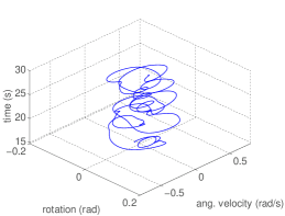
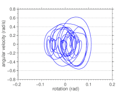
Figure 9: Projections of rotational dynamics phase space trajectories. (a) $\displaystyle\phi_{1}$ atractor in $\displaystyle\mathbb{R}^{3}$; (b) $\displaystyle\phi_{2}$ atractor in $\displaystyle\mathbb{R}^{3}$; (c) $\displaystyle\phi_{1}$ atractor in $\displaystyle\mathbb{R}^{2}$; (d) $\displaystyle\phi_{2}$ atractor in $\displaystyle\mathbb{R}^{2}$.

Finally, the time series corresponding to the tower horizontal dynamics $\displaystyle x_{2}$, which is the main QoI associated to the dynamic system under study, is shown in Figure 10, and the associated phase space trajectories projections are presented in Figure 11. An irregular dynamics that accumulates into a strange attractor is noticed once more.

A parametric study on the behavior of $\displaystyle x_{2}$, for different values of correlation length $\displaystyle a_{corr}$ and translation velocity $\displaystyle v$ can be seen in Figures 10 and 10, respectively. Note that lateral oscillation amplitude strongly depends on the correlation length. This amplitude also depends on the translation velocity, in a way that it decreases as $\displaystyle v$ increases, but this dependence is weaker than the one with $\displaystyle a_{corr}$.

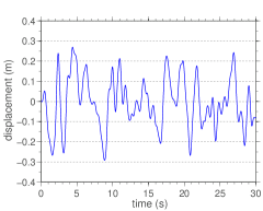
Figure 10: Time series of tower horizontal dynamics $\displaystyle x_{2}$. (a) nominal set of parameters; (b) several values of $\displaystyle a_{corr}$; (c) several values of $\displaystyle v$.

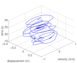
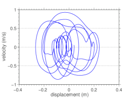
Figure 11: Projections of horizontal dynamics phase space trajectory. (a) $\displaystyle x_{2}$ attractor in $\displaystyle\mathbb{R}^{3}$; (b) $\displaystyle x_{2}$ attractor in $\displaystyle\mathbb{R}^{2}$.

4.3 Spectral analysis

In order to perform a spectral analysis of the dynamics, an estimation of the power spectral density (PSD) of the QoI signal is constructed using the periodogram method [29, 30]. In this algorithm, a wider interval of analysis is considered, for instance $\displaystyle[t_{0},t_{f}]=[0,6000]$ s, so that QoI time series is segmented into non-overlying windows, being the signal PSD constructed through an averaging process, which uses estimations of the PSD for each window of the segmented signal.

The PSD of tower horizontal displacement signal is presented in Figure 12, where it is possible to see that, for almost all the frequencies in the band of interest, $\displaystyle\mathcal{B}=[0,5]$ Hz, the signal energy follows a linear decreasing law, with inclination -2. This behavior, in form of a direct energy cascade, indicates that energy is injected in the system at the low frequencies of $\displaystyle\mathcal{B}$, being transferred in a nonlinear way through intermediate frequencies, until it is dissipated at the large frequencies by the structural damping.

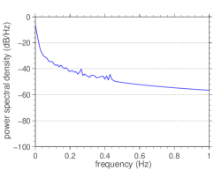
Figure 12: Power spectral density of tower horizontal displacement. (a) frequencies in linear scale. (b) frequencies in logarithmic scale.

4.4 Convergence of MC simulation

In order to ensure the “quality” of the statistics obtained from MC data, it is necessary to study the convergence of these stochastic simulations. For this purpose, it is taken into consideration the map conv, defined in section 3.6.

The evolution of $\displaystyle\texttt{conv}(n_{s})$ as a function of $\displaystyle n_{s}$ can be seen in Figure 13. Note that for $\displaystyle n_{s}=256$ the metric value has reached a steady value. So, all the stochastic simulations reported in this work use $\displaystyle n_{s}=256$.

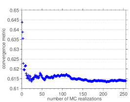
Figure 13: MC convergence metric as function of the realizations number.

Being the representative of the MC simulation guaranteed, an analysis of how uncertainties (due to randomness in the external loading) are propagated through the model is presented in the next sections.

4.5 Confidence band and low order statistics

In Figure 14 are presented some realizations of tower horizontal displacement and the corresponding confidence band (grey shadow), wherein a realization of the stochastic system has 95% of probability of being contained. A wide variability in the QoI form can be observed. This fact may also be noted in Figure 15, which shows the evolution of the QoI sample mean and standard deviation. Note that $\displaystyle x_{2}$ has mean value near zero, but significant variability near all the interval of analysis.

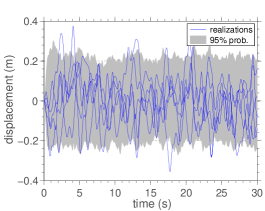
Figure 14: Confidence envelope and some realizations for tower horizontal displacement.

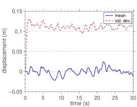
Figure 15: Sample mean/standard deviation for tower horizontal displacement.

4.6 Evolution of tower horizontal vibration PDF

Estimations for the normalized probability density function (PDF) of the tower horizontal vibration, for different instants of time, are presented in Figure 16. In all cases it is possible to observe small asymmetries with respect to mean and unimodal behavior, with maximum always occurring in the neighborhood of the mean value. The time average of the tower horizontal dynamics PDF is shown in Figure 17, which reflects the unimodal characteristic of $\displaystyle x_{2}$ distribution observed in the time instants of Figure 16.

(a) $\displaystyle t=7.5\,s$

(b) $\displaystyle t=15.0\,s$

(c) $\displaystyle t=22.5\,s$

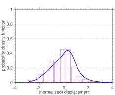
(d) $\displaystyle t=30.0\,s$

Figure 16: Probability density function of tower horizontal dynamics (at different instants).

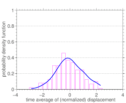
Figure 17: Time average of tower horizontal dynamics probability density function.

4.7 Large vibrations probability

When the uncertainties in orchard sprayer dynamics are quantified through a probabilistic approach, it is of particular interest to calculate the probability of occurrence of extreme events. For instance, the structure presents large lateral (horizontal) vibrations due to some extreme loading or as a consequence of nonlinear interactions between the soil irregularities and the tower sprayer.

To perform this calculation it is necessary to define a level of lateral vibration that is considered high. In this paper, this value corresponds to an amplitude of lateral vibration greater than 30% of the distance between the left wheel and the trailer center line, i.e.,

$$\text{large vibration}=\left\{\mid\mathbb{x}_{2}(t)\mid\leavevmode\nobreak\ >\leavevmode\nobreak\ \mbox{30\% of $\displaystyle B_{1}$}\right\}.$$ (95)

Therefore, for any instant $\displaystyle t$, it is of interest to determine the value of

$$\mathbb{P}\left\{\mid\mathbb{x}_{2}(t)\mid\leavevmode\nobreak\ >\leavevmode\nobreak\ \mbox{30\% of $\displaystyle B_{1}$}\right\}=1-\mathbb{P}\left\{\mid\mathbb{x}_{2}(t)\mid\leavevmode\nobreak\ \leq\leavevmode\nobreak\ \mbox{30\% of $\displaystyle B_{1}$}\right\},$$ (96)

where

$$\mathbb{P}\left\{\mid\mathbb{x}_{2}(t)\mid\leavevmode\nobreak\ \leq\leavevmode\nobreak\ \mbox{30\% of $\displaystyle B_{1}$}\right\}=\int_{-0.3\,B_{1}}^{+0.3\,B_{1}}dF_{\tiny{\mathbb{x}_{2}(t)}}(x_{2}).$$ (97)

The last integral corresponds to the area of the curve that represents the PDF of $\displaystyle x_{2}(t)$, above the interval $\displaystyle\left[-0.3\,B_{1},0.3\,B_{1}\right]$. By calculating the integral of Eq.(97) for every instant in the time interval of analysis, and then replacing the result in Eq.(96), the probability of large lateral vibrations as a function of time is obtained. The evolution of this probability is shown in Figure 18, where the reader can note that the probability of an unwanted level of lateral vibration is not negligible in general (20% on average), with peaks values near 40%.

Figure 18: Evolution of the probability of large horizontal vibrations.

5 Conclusions

This work presented the study of the nonlinear dynamics of an orchard tower sprayer that is subjected to random excitations due to soil irregularities, modeled as a three degrees of freedom multibody system. The random loadings were taken into account through a parametric probabilistic approach, where the external loading was assumed to be a random process that is represented through Karhunen-Loève decomposition. The paper not only proposes a mechanical analysis, but also provides a formulation for this type of system, and a methodology, that can be reused to analyze other industrial equipment excited by soil irregularities induced loads.

Numerical simulations showed that orchard tower sprayer has a very rich nonlinear dynamics, which is able to reproduce complex phenomena such as chaos. The study also indicated that system dynamics follows a direct energy cascade law, where the energy injected at the low frequencies are transferred into a nonlinear way through the middle frequencies of the band, being dissipated at the high frequencies.

A probabilistic analysis discloses a wide range of possible responses for the mechanical system, and shows a non negligible possibility of large lateral vibrations being developed during the sprayer operation.

In a future work, the authors intend to address the problem of lateral vibrations from the robust optimization point of view. Using the stochastic model developed in this work, they intend to find a robust strategy to change pair of system parameters (e.g., torsional stiffness and damping) in a way the levels of lateral vibrations are reduced. In parallel, it would be interesting to study the possibility of internal resonances, and to verify how they may disrupt or help in the operation of sprayer tower.

Author contributions

J.M.B. proposed the problematic. A.C. and J.M.B. designed the research plan. J.M.B and J.L.P.F. constructed the deterministic model, based on a previous work of then. A.C. constructed an original stochastic model. J.L.P.F. implemented a deterministic version of the computational code, which was extended and adapted to run stochastic simulations by A.C. Numerical simulations were carried out by A.C.. All the authors interpreted and discussed the results. A.C. wrote the manuscript, which was then revised by J.L.P.F. and J.M.B.. All authors approved the final manuscript.

References

References

- [1] S. Sartori Junior, J. M. Balthazar, B. R. Pontes Junior, Non-linear dynamics of a tower orchard sprayer based on an inverted pendulum model, Biosystems Engineering 103 (2009) 417–426.
- [2] S. Sartori Junior, Mathematical modeling and dynamic analysis of a orchards spray tower, M.Sc. Dissertation, Universidade Estadual Paulista Julio de Mesquita Filho, Bauru, (in portuguese) (2008).
- [3] S. Sartori Junior, M. Balthazar, B. R. Pontes, Nonlinear dynamics of an orchard tower sprayer based on a double inverted pendulum model, In: Proceedings of COBEM 2007, Brasilia, 2007.
- [4] C. Soize, Stochastic Models of Uncertainties in Computational Mechanics, American Society of Civil Engineers, Reston, 2012.
- [5] C. Soize, Stochastic modeling of uncertainties in computational structural dynamics — recent theoretical advances, Journal of Sound and Vibration 332 (2013) 2379–2395.
- [6] A. Cunha Jr, C. Soize, R. Sampaio, Computational modeling of the nonlinear stochastic dynamics of horizontal drillstrings, Computational Mechanics (2015) 849–878.
- [7] A. Cunha Jr, R. Sampaio, On the nonlinear stochastic dynamics of a continuous system with discrete attached elements, Applied Mathematical Modelling 39 (2015) 809–819.
- [8] G. Perrin, D. Duhamel, C. Soize, C. Funfschilling, Quantification of the influence of the track geometry variability on the train dynamics, Mechanical Systems and Signal Processing 60 (2015) 945–957.
- [9] T. G. Ritto, L. C. S. Nunes, Bayesian model selection of hyperelastic models for simple and pure shear at large deformations, Computers & Structures 156 (2015) 101–109.
- [10] A. T. Beck, W. J. S. Gomes, R. H. Lopez, L. F. F. Miguel, A comparison between robust and risk-based optimization under uncertainty, Structural and Multidisciplinary Optimization 52 (2015) 479–492.
- [11] A. Cunha Jr, J. L. P. Felix, J. M. Balthazar, On the nonlinear dynamics of an inverted double pendulum over a vehicle suspension subject to random excitations, In: Proceedings of COBEM 2015, Rio de Janeiro, 2015.
- [12] A. Cunha Jr, J. L. P. Felix, J. M. Balthazar, Effects of a random loading emulating an irregular terrain in the nonlinear dynamics of a tower sprayer, In: Proceedings of Uncertainties 2016, São Sebastião, 2016.
- [13] E. Fehlberg, Low-order classical Runge-Kutta formulas with step size control and their application to some heat transfer problems, Technical Report, NASA Technical Report 315 (1969).
- [14] U. Ascher, C. Greif, A First Course in Numerical Methods, Society for Industrial and Applied Mathematics, Philadelphia, 2011.
- [15] D. Xiu, Numerical Methods for Stochastic Computations: A Spectral Method Approach, Princeton University Press, Princeton, 2010.
- [16] R. Ghanem, P. Spanos, Stochastic Finite Elements: A Spectral Approach, Dover Publications, New York, 2003.
- [17] S. Bellizzi, R. Sampaio, POMs analysis of randomly vibrating systems obtained from Karhunen–Loève expansion, Journal of Sound and Vibration 297 (2006) 774–793.
- [18] R. Sampaio, C. Soize, Remarks on the efficiency of POD for model reduction in non-linear dynamics of continuous elastic systems, International Journal of Numerical Methods in Engineering 72 (2007) 22–45.
- [19] G. Stefanou, M. Papadrakakis, Assessment of spectral representation and Karhunen–Loève expansion methods for the simulation of Gaussian stochastic fields, Computer Methods in Applied Mechanics and Engineering 196 (2007) 2465–2477.
- [20] S. Bellizzi, R. Sampaio, Smooth Karhunen–Loève decomposition to analyze randomly vibrating systems, Journal of Sound and Vibration 325 (2009) 491–498.
- [21] S. Bellizzi, R. Sampaio, Karhunen–Loève modes obtained from displacement and velocity fields: assessments and comparisons, Mechanical Systems and Signal Processing 23 (2009) 1218–1222.
- [22] S. Bellizzi, R. Sampaio, Smooth decomposition of random fields, Journal of Sound and Vibration 331 (2012) 3509–3520.
- [23] S. Bellizzi, R. Sampaio, The smooth decomposition as a nonlinear modal analysis tool, Mechanical Systems and Signal Processing 64–65 (2015) 245–256.
- [24] M. Trindade, C. Wolter, R. Sampaio, Karhunen–Loève decomposition of coupled axial/bending vibrations of beams subject to impacts, Journal of Sound and Vibration 279 (2005) 1015–1036.
- [25] D. P. Kroese, T. Taimre, Z. I. Botev, Handbook of Monte Carlo Methods, Wiley, New Jersey, 2011.
- [26] A. Cunha Jr, R. Nasser, R. Sampaio, H. Lopes, K. Breitman, Uncertainty quantification through Monte Carlo method in a cloud computing setting, Computer Physics Communications 185 (2014) 1355-–1363.
- [27] C. Soize, A comprehensive overview of a non-parametric probabilistic approach of model uncertainties for predictive models in structural dynamics, Journal of Sound and Vibration 288 (2005) 623–652.
- [28] https://youtu.be/9thgNv3U_uM, (accessed 2017.06.05).
- [29] A. V. Oppenheim, R. W. Schafer, Discrete-Time Signal Processing, 3rd Edition, Prentice Hall, Englewood Cliffs, 2009.
- [30] C. Soize, Fundamentals of random signal analysis: Application to modal identification in structural dynamics, Lecture Notes, University of Marne-la-Vallée, Paris (1997).