Sparse formulae for the distance modulus in cosmology

Abstract

We review the distance modulus in twelve different cosmologies: the $\Lambda$CDM model, the wCDM model, the Cardassian model, the flat case, the $\phi$CDM cosmology, the Einstein–De Sitter model, the modified Einstein–De Sitter model, the simple GR model, the flat expanding model, the Milne model, the plasma model and the modified tired light model. The above distance moduli are processed for three different compilations of supernovae and a supernovae + GRBs compilation: Union 2.1, JLA, the Pantheon and Union 2.1 + 59 GRBs. For each of the 48 analysed cases we report the relative cosmological parameters, the chi-square, the reduced chi-square, the AIC and the $Q$ parameter. The angular distance as function of the redshift for five cosmologies is reported in the framework of the minimax approximation.

Keywords : Cosmology; Observational cosmology; Distances, redshifts, radial velocities, spatial distribution of galaxies; Magnitudes and colours, luminosities

1 Introduction

At the moment of writing, the determination of the Hubble constant is oscillating between a low value as derived by the Planck collaboration [1], $H_{0}=(67.4\pm 0.5)\mathrm{km\,s^{-1}\,Mpc^{-1}}$, and an high value, $H_{0}=(74.03\pm 1.42)\mathrm{km\,s^{-1}\,Mpc^{-1}}$, as measured on 70 long-period Cepheids in the Large Magellanic Cloud (LMC)[2]. The above difference is referred to as the Hubble constant tension [3] and takes the value of $4.4\sigma$. It fixes an acceptable interval for the evaluation of $H_{0}$. The number of supernovae (SNs) of type Ia for which the distance modulus is available has grown with time: 34 SNs in the sample which produced evidence for the accelerating universe [4], 580 SNs in the Union 2.1 compilation [5], 740 SNs in the joint light-curve analysis (JLA) [6], and 1048 SNs in the Pantheon sample [7, 8]. The availability of SN compilations allows testing old and new cosmological models. We select some of them among others: cosmological relativity in five spatial dimensions [9], an improvement of the Einstein–De Sitter cosmology [10], the $f(R)$ gravity with additional logarithmic corrections [11, 12], influence of the detection of gravitational waves on a definitive theory of gravity [13], the derivation of the value of the Hubble constant as $H_{0}=(70.5\pm 0.5)\mathrm{km\,s^{-1}\,Mpc^{-1}}$ in the framework of the dark energy cosmology [14] and the deduction of the parameters for Starobinsky gravity [15]. This paper reviews, in Section 2, old and new distance moduli in twelve cosmologies. Then Section 3 processes the analysed cosmologies in four compilations of SNs.

2 Different cosmologies

In the following we analyse twelve cosmologies. A useful introduction to the distances in cosmology can be found in [16].

2.1 The standard cosmology

In $\Lambda$CDM cosmology the Hubble distance $D_{\rm H}$ is defined as

$$D_{\rm H}\equiv\frac{c}{H_{0}}\quad,$$ (1)

where $c$ is the speed of light and $H_{0}$ is the Hubble constant. We then introduce a first parameter $\Omega_{\rm M}$

$$\Omega_{\rm M}=\frac{8\pi\,G\,\rho_{0}}{3\,H_{0}^{2}}\quad,$$ (2)

where $G$ is the Newtonian gravitational constant and $\rho_{0}$ is the mass density at the present time. A second parameter is $\Omega_{\Lambda}$

$$\Omega_{\Lambda}\equiv\frac{\Lambda\,c^{2}}{3\,H_{0}^{2}}\quad,$$ (3)

where $\Lambda$ is the cosmological constant, see [17]. Once $\Omega_{\Lambda}$ and $H_{0}$ are found the numerical value of the cosmological constant is derived, $\Lambda\approx 1.2\frac{1}{m^{2}}$.

The two previous parameters are connected with the curvature $\Omega_{K}$ by

$$\Omega_{\rm M}+\Omega_{\Lambda}+\Omega_{K}=1\quad.$$ (4)

The comoving distance, $D_{\rm C}$, is

$$D_{\rm C}=D_{\rm H}\,\int_{0}^{z}\frac{dz^{\prime}}{E(z^{\prime})}\quad,$$ (5)

where $E(z)$ is the ‘Hubble function’

$$E(z)=\sqrt{\Omega_{\rm M}\,(1+z)^{3}+\Omega_{K}\,(1+z)^{2}+\Omega_{\Lambda}}\quad.$$ (6)

The above integral cannot be done in analytical terms, except for the case of $\Omega_{\Lambda}=0$, but the Padé approximant, see Appendix A, allows to derive the approximated indefinite integral, see equation (A.10).

The approximate definite integral for (5) is therefore

$$D_{\rm C,2,2}=D_{\rm H}\,\Big{(}F_{2,2}(z;a_{0},a_{1},a_{2},b_{0},b_{1},b_{2})-F_{2,2}(0;a_{0},a_{1},a_{2},b_{0},b_{1},b_{2})\Big{)}\quad,$$ (7)

where $F_{2,2}$ is equation (A.10). The transverse comoving distance $D_{\rm M}$ is

$$D_{\rm M}=\left\{\begin{array}[]{ll}D_{\rm H}\,\frac{1}{\sqrt{\Omega_{K}}}\,\sinh\left[\sqrt{\Omega_{K}}\,D_{\rm C}/D_{\rm H}\right]&{\rm for}~{}\Omega_{K}>0\\ D_{\rm C}&{\rm for}~{}\Omega_{K}=0\\ D_{\rm H}\,\frac{1}{\sqrt{|\Omega_{K}|}}\,\sin\left[\sqrt{|\Omega_{K}|}\,D_{\rm C}/D_{\rm H}\right]&{\rm for}~{}\Omega_{K}<0\end{array}\right.$$ (8)

and the approximate transverse comoving distance $D_{\rm M,2,2}$ computed with the Padé approximant is

$$D_{\rm M,2,2}=\left\{\begin{array}[]{ll}D_{\rm H}\,\frac{1}{\sqrt{\Omega_{K}}}\,\sinh\left[\sqrt{\Omega_{K}}\,D_{\rm C,2,2}/D_{\rm H}\right]&{\rm for}~{}\Omega_{K}>0\\ D_{\rm C,2,2}&{\rm for}~{}\Omega_{K}=0\\ D_{\rm H}\,\frac{1}{\sqrt{|\Omega_{K}|}}\,\sin\left[\sqrt{|\Omega_{K}|}\,D_{\rm C,2,2}/D_{\rm H}\right]&{\rm for}~{}\Omega_{K}<0\end{array}\right.$$ (9)

The Padé approximant for the luminosity distance is

$$D_{\rm L,2,2}=(1+z)\,D_{\rm M,2,2}\quad,$$ (10)

and the Padé approximant for the distance modulus, $(m-M)_{2,2}$, is

$$(m-M)_{2,2}=25+5\log_{10}(D_{\rm L,2,2})\quad.$$ (11)

As a consequence, $M_{2,2}$, the absolute magnitude of the Padé approximant, is

$$M_{2,2}=m-25-5\log_{10}(D_{\rm L,2,2})\quad.$$ (12)

The expanded version of the Padé approximant distance modulus is

$$(m-M)_{2,2}=$$

$$25+5\,{\frac{1}{\ln\left(10\right)}\ln\left({\frac{c\left(1+z\right)}{H_{{0}}\sqrt{{\it\Omega_{K}}}}\sinh\left(1/2\,{\frac{\sqrt{{\it\Omega_{K}}}A}{{b_{{2}}}^{2}\sqrt{4\,b_{{0}}b_{{2}}-{b_{{1}}}^{2}}}}\right)}\right)}\quad,$$ (13)

with

$$A=\ln\left({z}^{2}b_{{2}}+zb_{{1}}+b_{{0}}\right)a_{{1}}b_{{2}}\sqrt{4\,b_{{0}}b_{{2}}-{b_{{1}}}^{2}}$$

$$-\ln\left({z}^{2}b_{{2}}+zb_{{1}}+b_{{0}}\right)a_{{2}}b_{{1}}\sqrt{4\,b_{{0}}b_{{2}}-{b_{{1}}}^{2}}$$

$$-\ln\left(b_{{0}}\right)a_{{1}}b_{{2}}\sqrt{4\,b_{{0}}b_{{2}}-{b_{{1}}}^{2}}$$

$$+\ln\left(b_{{0}}\right)a_{{2}}b_{{1}}\sqrt{4\,b_{{0}}b_{{2}}-{b_{{1}}}^{2}}+2\,a_{{2}}zb_{{2}}\sqrt{4\,b_{{0}}b_{{2}}-{b_{{1}}}^{2}}$$

$$+4\,\arctan\left({\frac{2\,zb_{{2}}+b_{{1}}}{\sqrt{4\,b_{{0}}b_{{2}}-{b_{{1}}}^{2}}}}\right)a_{{0}}{b_{{2}}}^{2}-2\,\arctan\left({\frac{2\,zb_{{2}}+b_{{1}}}{\sqrt{4\,b_{{0}}b_{{2}}-{b_{{1}}}^{2}}}}\right)b_{{1}}a_{{1}}b_{{2}}$$

$$-4\,\arctan\left({\frac{2\,zb_{{2}}+b_{{1}}}{\sqrt{4\,b_{{0}}b_{{2}}-{b_{{1}}}^{2}}}}\right)a_{{2}}b_{{0}}b_{{2}}+2\,\arctan\left({\frac{2\,zb_{{2}}+b_{{1}}}{\sqrt{4\,b_{{0}}b_{{2}}-{b_{{1}}}^{2}}}}\right){b_{{1}}}^{2}a_{{2}}$$

$$-4\,\arctan\left({\frac{b_{{1}}}{\sqrt{4\,b_{{0}}b_{{2}}-{b_{{1}}}^{2}}}}\right)a_{{0}}{b_{{2}}}^{2}+2\,\arctan\left({\frac{b_{{1}}}{\sqrt{4\,b_{{0}}b_{{2}}-{b_{{1}}}^{2}}}}\right)b_{{1}}a_{{1}}b_{{2}}$$

$$+4\,\arctan\left({\frac{b_{{1}}}{\sqrt{4\,b_{{0}}b_{{2}}-{b_{{1}}}^{2}}}}\right)a_{{2}}b_{{0}}b_{{2}}-2\,\arctan\left({\frac{b_{{1}}}{\sqrt{4\,b_{{0}}b_{{2}}-{b_{{1}}}^{2}}}}\right){b_{{1}}}^{2}a_{{2}}$$

Figure 1 reports the percentage error, see formula (75), for $(m-M)_{2,2}$ as function of the redshift until the value of $1\%$ is reached at $z\approx 6$. For $z>6$ the Padé approximant of the distance modulus does not converge to the numerical distance modulus.

Figure 1: Percentage error of $(m-M)_{2,2}$ in respect to the numerical value with data as in Table 1.

More details can be found in [18].

2.2 Dynamical dark energy or wCDM

In the dynamical dark energy cosmology (wCDM), firstly introduced by [19], the Hubble distance is

$$D_{H}(z;\Omega_{\rm M},w,\Omega_{DE})=\frac{1}{\sqrt{\left(1+z\right)^{3}{\it\Omega_{\rm M}}+{\it\Omega_{DE}}\,\left(1+z\right)^{3+3\,w}}}\quad,$$ (14)

where $w$ is the equation of state here considered constant, see equation (3.4) in [20] or equation(18) in [21] for the luminosity distance. Here we considered $w$ to be constant but also the case of $w$ as function of $z$ can be considered, see equation (19) in [21]. In the above cosmology the cosmological constant is absent. In flat cosmology

$$\Omega_{\rm M}+\Omega_{DE}=1\quad,$$ (15)

and the Hubble distance becomes

$$D_{H}(z;\Omega_{\rm M},w)=\frac{1}{\sqrt{\left(1+z\right)^{3}{\it\Omega_{\rm M}}+\left(1-{\it\Omega_{\rm M}}\right)\left(1+z\right)^{3+3\,w}}}\quad.$$ (16)

The indefinite integral in the variable $z$ of the above Hubble distance, $Iz\equiv\frac{D_{C}}{D_{H}}$, is

$$Iz(z;\Omega_{\rm M},w)=\int D_{H}(z;\Omega_{\rm M},w)dz\quad,$$ (17)

where the new symbol $Iz$ underline the mathematical operation of integration. In order to solve for the the indefinite integral we perform a change of variable $1+z=t^{1/3}$

$$Iz(t;\Omega_{\rm M},w)=\frac{1}{3}\int\!{\frac{1}{\sqrt{-t\left(\left(-1+{\it\Omega_{\rm M}}\right){t}^{w}-{\it\Omega_{\rm M}}\right)}{t}^{2/3}}}\,{\rm d}t\quad.$$ (18)

The indefinite integral is

$$Iz(t;\Omega_{\rm M},w)=\frac{-2\,{\mbox{${}_{2}$F${}_{1}$}(\frac{1}{2},-\frac{1}{6}\,{w}^{-1};\,1-\frac{1}{6}\,{w}^{-1};\,-{\frac{{t}^{w}-\left(1-{\it\Omega_{\rm M}}\right)}{{\it\Omega_{\rm M}}}})}}{\sqrt{{\it\Omega_{\rm M}}}\sqrt[6]{t}}\quad,$$ (19)

where ${{}_{2}F_{1}(a,b;\,c;\,z)}$ is the regularized hypergeometric function, see [22, 23, 24, 25, 26]. We now return to the variable $z$, the redshift. Then the indefinite integral becomes

$$Iz(z;\Omega_{\rm M},w)=$$

$$\frac{-2\,{\mbox{${}_{2}$F${}_{1}$}(\frac{1}{2},-\frac{1}{6}\,{w}^{-1};\,1-\frac{1}{6}\,{w}^{-1};\,-{\frac{\left(-{z}^{3}+3\,{z}^{2}+3\,z+1\right)^{w}\left(1-{\it\Omega_{\rm M}}\right)}{{\it-\Omega_{\rm M}}}})}}{\sqrt{{\it\Omega_{\rm M}}}\sqrt[6]{{z}^{3}+3\,{z}^{2}+3\,z+1}}\quad.$$ (20)

We denote by $F(z;\Omega_{\rm M},w)$ the definite integral

$$F(z;\Omega_{\rm M},w)=Iz(z=z;\Omega_{\rm M},w)-Iz(z=0;\Omega_{\rm M},w)\quad.$$ (21)

The luminosity distance, $D_{\rm{L}}$, for wCDM cosmology in the case of the analytical solution is

$$D_{\rm{L}}(z;c,H_{0},\Omega_{\rm M},w)=\frac{c}{H_{0}}(1+z)F(z;\Omega_{\rm M},w)\quad,$$ (22)

where $F(z;\Omega_{\rm M},w)$ is given by equation (21) and the distance modulus is

$$(m-M)=25+5\log_{10}\bigg{(}D_{\rm{L}}(z;c,H_{0},\Omega_{\rm M},w)\bigg{)}\quad.$$ (23)

More details can be found in [27].

2.3 The Cardassian cosmology

In flat Cardassian cosmology [28, 29] the Hubble distance is

$$D_{H}(z;\Omega_{\rm M},w,n)={\frac{1}{\sqrt{\left(1+z\right)^{3}{\it\Omega_{\rm M}}+\left(1-{\it\Omega_{\rm M}}\right)\left(1+z\right)^{3\,n}}}}\quad,$$ (24)

where $n$ is a variable parameter, and $n=0$ means the $\Lambda$CDM cosmology, see equation (17) in [21]. The above equation can also be obtained inserting $n=1+w$ in equation (14). Despite of this fact the FORTRAN code which derives the cosmological parameters produces a small difference in the results because the variables are evaluated in a different way. The indefinite integral in the variable $z$ of the above Hubble distance, $Iz$, is

$$Iz(z;\Omega_{\rm M},n)=\int D_{H}(z;\Omega_{\rm M},n)dz\quad.$$ (25)

In order to obtain the indefinite integral we perform a change of variable $1+z=t^{1/3}$

$$Iz(t;\Omega_{\rm M},n)=\frac{1}{3}\int\!{\frac{1}{\sqrt{-{t}^{n}{\it\Omega_{\rm M}}+{\it\Omega_{\rm M}}\,t+{t}^{n}}{t}^{2/3}}}\,{\rm d}t\quad.$$ (26)

The indefinite integral is

$$Iz(t;\Omega_{\rm M},n)=\frac{-2\,{\mbox{${}_{2}$F${}_{1}$}\Big{(}1/2,-\left(6\,n-6\right)^{-1};\,{\frac{6\,n-7}{6\,n-6}};\,{\frac{{t}^{n-1}\left({\it\Omega_{\rm M}}-1\right)}{{\it\Omega_{\rm M}}}}\Big{)}}}{\sqrt{{\it\Omega_{\rm M}}}\sqrt[6]{t}}\quad,$$ (27)

where ${{}_{2}F_{1}(a,b;\,c;\,z)}$ is the regularized hypergeometric function. We now return to the original variable $z$ and the indefinite integral is

$$Iz(z;\Omega_{\rm M},n)=$$

$$\frac{-2\,{\mbox{${}_{2}$F${}_{1}$}\Big{(}1/2,-\left(6\,n-6\right)^{-1};\,{\frac{6\,n-7}{6\,n-6}};\,{\frac{\left(\left(1+z\right)^{3}\right)^{n-1}\left({\it\Omega_{\rm M}}-1\right)}{{\it\Omega_{\rm M}}}}\Big{)}}}{\sqrt{{\it\Omega_{\rm M}}}\sqrt[6]{\left(1+z\right)^{3}}}\quad.$$ (28)

We denote by $F_{c}(z;\Omega_{\rm M},n)$ the definite integral

$$F_{c}(z;\Omega_{\rm M},n)=Iz(z=z;\Omega_{\rm M},n)-Iz(z=0;\Omega_{\rm M},n)\quad.$$ (29)

In the case of the Cardassian cosmology, the luminosity distance is

$$D_{\rm{L}}(z;c,H_{0},\Omega_{\rm M},n)=\frac{c}{H_{0}}(1+z)F_{c}(z;\Omega_{\rm M},n)\quad,$$ (30)

where $F_{c}(z;\Omega_{\rm M},n)$ is given by equation (29) and the distance modulus is

$$(m-M)=25+5\log_{10}\bigg{(}D_{\rm{L}}(z;c,H_{0},\Omega_{\rm M},n)\bigg{)}\quad.$$ (31)

In the flat Cardassian cosmology, there are three parameters: $H_{0},\Omega_{\rm M}$ and $n$. More details can be found in [27].

2.4 The flat cosmology

The starting point is equation (1) for the luminosity distance in [30]

$$D_{\rm{L}}(z;c,H_{0},\Omega_{\rm M})=\frac{c(1+z)}{H_{0}}\int_{0}^{z}\!{\frac{1}{\sqrt{{\it\Omega_{\rm M}}\,\left(1+t\right)^{3}+1-{\it\Omega_{\rm M}}}}}\,{\rm d}t\quad,$$ (32)

where the variable of integration, $t$, denotes the redshift.

A first change in the parameter $\Omega_{\rm M}$ introduces

$$s=\sqrt[3]{{\frac{1-{\it\Omega_{\rm M}}}{{\it\Omega_{\rm M}}}}}\quad$$ (33)

and the luminosity distance becomes

$$D_{\rm{L}}(z;c,H_{0},s)=\frac{1}{H_{0}}c\left(1+z\right)\int_{0}^{z}\!{\frac{1}{\sqrt{{\frac{\left(1+t\right)^{3}}{{s}^{3}+1}}+1-\left({s}^{3}+1\right)^{-1}}}}\,{\rm d}t\quad.$$ (34)

The following change of variable, $t=\frac{s-u}{u}$, is performed for the luminosity distance, which becomes

$$D_{\rm{L}}(z;c,H_{0},s)=$$

$$-\frac{c}{{\it H_{0}}\,{s}^{2}}\left(1+z\right)\left({s}^{3}+1\right)\int_{s}^{{\frac{s}{1+z}}}\!{\frac{u}{{u}^{3}+1}\sqrt{{\frac{{s}^{3}\left({u}^{3}+1\right)}{{u}^{3}\left({s}^{3}+1\right)}}}}\,{\rm d}u\quad.$$ (35)

The integral for the luminosity distance is

$$D_{\rm{L}}(z;c,H_{0},s)=-1/3\,{\frac{c(1+z){3}^{3/4}\sqrt{{s}^{3}+1}}{\sqrt{s}{\it H_{0}}}}\times$$

$${\Bigg{(}{\it F}(2\,{\frac{\sqrt{s(s+1+z)}\sqrt[4]{3}}{s\sqrt{3}+s+z+1}},1/4\,\sqrt{2}\sqrt{3}+1/4\,\sqrt{2})}$$

$${-{\it F}(2\,{\frac{\sqrt[4]{3}\sqrt{s(s+1)}}{s+1+s\sqrt{3}}},1/4\,\sqrt{2}\sqrt{3}+1/4\,\sqrt{2})\Bigg{)}}\quad,$$ (36)

where $s$ is given by Eq. (33) and $F\left(\phi,k\right)$ is Legendre’s incomplete elliptic integral of the first kind,

$$F\left(\phi,k\right)=\int_{0}^{\sin\phi}\frac{\mathrm{d}t}{\sqrt{1-t^{2}}\sqrt{1-k^{2}t^{2}}}\quad,$$ (37)

see [26]. The distance modulus is

$$(m-M)=25+5\log_{10}\bigg{(}D_{\rm{L}}(z;c,H_{0},s)\bigg{)}\quad,$$ (38)

and therefore

$$(m-M)=25$$

$$+5\,{\frac{1}{\ln\left(10\right)}\ln\left(-\frac{1}{3}\,{\frac{c\left(1+z\right){3}^{3/4}\left({\it F_{1}}-{\it F_{2}}\right)\sqrt{{s}^{3}+1}}{\sqrt{s}{\it H_{0}}}}\right)}\quad,$$ (39)

where

$$F_{1}={\it F}\left(2\,{\frac{\sqrt{s\left(s+1+z\right)}\sqrt[4]{3}}{s\sqrt{3}+s+z+1}},1/4\,\sqrt{2}\sqrt{3}+1/4\,\sqrt{2}\right)$$ (40)

and

$$F_{2}={\it F}\left(2\,{\frac{\sqrt[4]{3}\sqrt{s\left(s+1\right)}}{s+1+s\sqrt{3}}},1/4\,\sqrt{2}\sqrt{3}+1/4\,\sqrt{2}\right)\quad,$$ (41)

with $s$ as defined by Eq. (33). More details can be found in [31].

2.5 $\phi$CDM cosmology

The inflationary universe has been introduced by [32, 33, 34] and the term ”quintessence” in a title of a paper appeared in [35]. At the moment of writing given a scalar field, $\phi$, and the connected self-interacting potential, $V(\phi)$, ten different quintessence models are suggested by [36]. Here we start from equation (12) in [37] where $E(z)$, the ‘Hubble function’, is

$$E(z;\Omega_{\rm M0},\Omega_{\rm\phi\,0}\alpha\beta)=\sqrt{\left(1+z\right)^{3}{\it\Omega_{\rm M0}}+{\it\Omega_{\rm\phi\,0}}\,\left(1+z\right)^{\alpha}{{\rm e}^{\beta\,z}}}\quad,$$ (42)

where $\Omega_{\rm M0}=\frac{\rho_{m0}}{3H_{0}^{2}}$ is the adimensional present density of matter, $\Omega_{\rm\phi\,0}=\frac{\rho_{\phi\,0}}{3H_{0}^{2}}$ is the present adimensional density of the scalar field, $H_{0}$ is the present value of the Hubble constant, $\rho_{m0}$ is the present density of matter, $\rho_{\phi\,0}$ is the present density of the scalar field, $\alpha$ and $\beta$ are two parameters which allow to match theory and observations. In absence of curvature we have

$$\Omega_{\rm M0}+\Omega_{\rm\phi\,0}=1\quad,$$ (43)

and therefore

$$E(z;\Omega_{\rm M0},\alpha,\beta)=\sqrt{\left(1+z\right)^{3}{\it\Omega_{\rm M0}}+\left(1-{\it\Omega_{\rm M0}}\right)\left(1+z\right)^{\alpha}{{\rm e}^{\beta\,z}}}\quad.$$ (44)

The luminosity distance is

$$D_{\rm{L}}(z;c,H_{0},\Omega_{\rm M0},\alpha,\beta)=\frac{c(1+z)}{H_{0}}\int_{0}^{z}\!\frac{1}{E(t;\Omega_{\rm M0},\alpha,\beta)}\,dt\quad,$$ (45)

where the variable of integration, $t$, denotes the redshift. At the moment of writing there is not an analytical solution for the above integral and therefore we implement a numerical solution, $D_{\rm{L,num}}(z;c,H_{0},\Omega_{\rm M0},\alpha,\beta)$. The distance modulus is

$$(m-M)=25+5\log_{10}\bigg{(}D_{\rm{L,num}}(z;c,H_{0},\Omega_{\rm M0},\alpha,\beta)\bigg{)}\quad.$$ (46)

An approximate value of the above integral (45) is obtained with a Taylor expansion of the integrand about $z=1$ of order seven denoted by $D_{\rm{L,7}}(z;c,H_{0},\Omega_{\rm M0},\alpha,\beta)$. We report the numerical expression with cosmological parameters as in Table 1 relative to the Union 2.1 compilation:

$$D_{\rm{L,7}}(z)=$$

$$4282.7\,\left(1+z\right)\Big{(}0.91287\,z-0.16562\,{z}^{2}+0.039001\,\left(z-1\right)^{3}$$

$$-0.003084\,\left(z-1\right)^{4}-0.0036858\,\left(z-1\right)^{5}+0.0028217\,\left(z-1\right)^{6}$$

$$-0.00115816\,\left(z-1\right)^{7}+0.03442\Big{)}\quad.$$ (47)

The approximate distance modulus is

$$(m-M)_{7}=25+5\log_{10}\bigg{(}D_{\rm{L,7}}(z;c,H_{0},\Omega_{\rm M0},\alpha,\beta)\bigg{)}\quad,$$ (48)

which for the Union 2.1 compilation has the following numerical expression

$$(m-M)_{7}=25$$

$$+\frac{5}{\ln(10)}\Bigg{(}\ln\Big{(}4282.7(1+z)(0.91287z-0.16562{z}^{2}+0.039001(z-1)^{3}$$

$$-0.0030847(z-1)^{4}-0.0036858(z-1)^{5}+0.0028217(z-1)^{6}$$

$$-0.0011581(z-1)^{7}+0.03442)\Big{)}\Bigg{)}\,.$$ (49)

Figure 2 reports the percentage error, see formula (75), for $(m-M)_{7}$ as function of the redshift until the value of $0.02\%$ is reached at $z\approx 2.5$.

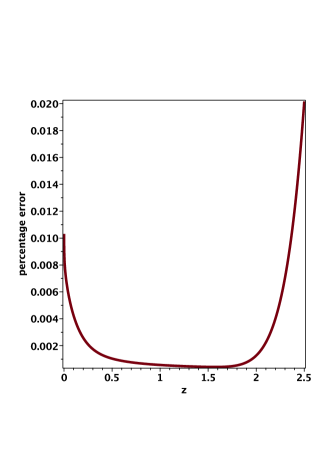
Figure 2: Percentage error of $(m-M)_{7}$ in respect to the numerical value with data as in Table 1.

2.6 The Einstein–De Sitter cosmology

In the Einstein–De Sitter model the luminosity distance,$D_{L}$, after [38, 39], is

$$D_{L}=2\,{\frac{c\left(1+z-\sqrt{z+1}\right)}{H_{{0}}}}\quad,$$ (50)

and the distance modulus for the Einstein–De Sitter model is

$$m-M=25+5\,{\frac{1}{\ln\left(10\right)}\ln\left(2\,{\frac{c\left(1+z-\sqrt{z+1}\right)}{H_{{0}}}}\right)}\quad.$$ (51)

There is one free parameter in the Einstein–De Sitter model: $H_{0}$. The Einstein–De Sitter model has been recently improved by [10], splitting the analysis in two: the Einstein–De Sitter flat, only-matter universe, referred to as EdesNa, and a flat, only-matter, including the Mach effect universe, referred to as EDSM. We limit ourselves to the EdesNA model and we start from equation (37) of [10]

$$m-M=5\,{\frac{\ln\left(5/3\,R_{{0}}\left(1+z\right){\it I_{G}(z)}\right)}{\ln\left(10\right)}}+25\quad,$$ (52)

where

$$R_{0}=\frac{c}{H_{0}}\quad,$$ (53)

and

$$I_{G}(z)=\int_{0}^{z}\frac{1}{1+{\frac{2}{3}\left(1+x\right)^{{\frac{3}{2}}}}}dx\quad.$$ (54)

Evaluating the integral yields

$$I_{G}(z)=-\sqrt[6]{3}\Bigg{(}\arctan({\frac{2\,\sqrt[6]{3}\sqrt[3]{2}}{3}}-{\frac{\sqrt{3}}{3}})$$

$$-\arctan({\frac{2\,\sqrt[6]{3}\sqrt[3]{2}}{3}\sqrt[3]{(1+z)^{{\frac{3}{2}}}}}-{\frac{\sqrt{3}}{3}})\Bigg{)}\sqrt[3]{2}-{\frac{{12}^{{\frac{2}{3}}}}{12}\Bigg{(}\ln(-\sqrt[3]{2}\sqrt[3]{3}+{2}^{{\frac{2}{3}}}+{3}^{{\frac{2}{3}}})}$$

$${-2\,\ln(\sqrt[3]{2}+\sqrt[3]{3})+2\,\ln(\sqrt[3]{2}{3}^{2/3}\sqrt[3]{(1+z)^{3/2}}+3)}$$

$${-\ln({2}^{{\frac{2}{3}}}\sqrt[3]{3}((1+z)^{{\frac{3}{2}}})^{{\frac{2}{3}}}-\sqrt[3]{2}{3}^{{\frac{2}{3}}}\sqrt[3]{(1+z)^{{\frac{3}{2}}}}+3)-\ln(3)\Bigg{)}}\quad.$$ (55)

The integrand of (54) can be approximated with a Padé approximant with $p=2,q=2$,

$$I_{G22}(z)=\int_{0}^{z}\frac{-3\,{x}^{2}+36\,x+144}{67\,{x}^{2}+204\,x+240}dx\quad,$$ (56)

and therefore we have the approximate integral

$$I_{G22}(z)=-{\frac{3\,z}{67}}+{\frac{1512\,\ln\left(67\,{z}^{2}+204\,z+240\right)}{4489}}$$

$$+{\frac{64368\,\sqrt{1419}}{2123297}\arctan\left({\frac{\left(134\,z+204\right)\sqrt{1419}}{5676}}\right)}-{\frac{1512\,\ln\left(240\right)}{4489}}$$

$$-{\frac{64368\,\sqrt{1419}\arctan\left({\frac{17\,\sqrt{1419}}{473}}\right)}{2123297}}\quad,$$ (57)

which generates the following approximate distance modulus

$$(m-M)_{22}=5\,{\frac{\ln\left(5/3\,R_{{0}}\left(1+z\right){\it I_{G22}(z)}\right)}{\ln\left(10\right)}}+25\quad.$$ (58)

The percent error between the approximate distance modulus as given by equation (58) and the the exact distance modulus as given by equation (52) is $\approx\,0.03\%$ when $z=4$ and $H_{0}=69.1$.

2.7 Simple GR cosmology

In the framework of GR, the received flux, $f$, is

$$f=\frac{L}{4\,\pi D_{L}^{2}}\quad,$$ (59)

where $D_{L}$ is the luminosity distance, which depends on the cosmological model adopted, see Eq. (7.21) in [40] or Eq. (5.235) in [41].

The distance modulus in the simple GR cosmology is

$$m-M=43.17-{\frac{1}{\ln\left(10\right)}\ln\left({\frac{{\it H_{0}}}{70}}\right)}+5\,{\frac{\ln\left(z\right)}{\ln\left(10\right)}}+1.086\,\left(1-{\it q_{0}}\right)z\quad,$$ (60)

see Eq. (7.52) in [40]. There are two free parameters in the simple GR cosmology: $H_{0}$ and $q_{0}$.

2.8 Flat expanding universe

This model is based on the standard definition of luminosity in the flat expanding universe. The luminosity distance, $r_{L}^{\prime}$, is

$$r_{L}^{\prime}=\frac{c}{H_{0}}z\quad,$$ (61)

and the distance modulus is

$$m-M==-5\log_{10}+5\log_{10}r_{L}^{\prime}+2.5\log(1+z)\quad,$$ (62)

see formulae (13) and (14) in [42]. There is one free parameter in the flat expanding model, $H_{0}$.

2.9 The Milne universe in SR

In the Milne model, which is developed in the framework of SR, the luminosity distance, after [43, 44, 45], is

$$D_{L}={\frac{c\left(z+\frac{1}{2}\,{z}^{2}\right)}{H_{{0}}}}\quad,$$ (63)

and the distance modulus for the Milne model is

$$m-M=25+5\,{\frac{1}{\ln\left(10\right)}\ln\left({\frac{c\left(z+\frac{1}{2}\,{z}^{2}\right)}{H_{{0}}}}\right)}\quad.$$ (64)

There is one free parameter in the Milne model: $H_{0}$.

2.10 Plasma cosmology

In an Euclidean static framework from among many possible absorption mechanisms, we have selected a plasma effect which produces the following relation for the distance $d$

$$d=\frac{c}{H_{0}}\ln(1+z)\quad,$$ (65)

where the distance expressed in lower case underline the difference with the relativistic case, see Eq. (50) in [46].

In the presence of plasma absorption, the observed flux is

$$f=\frac{{L\cdot\exp\left({-bd-H_{0}d-2H_{0}d}\right)}}{{4\pi d^{2}}}\quad,$$ (66)

where the factor $\exp\left({-bd}\right)$ is due to galactic and host galactic extinctions, $-H_{0}d$ is the reduction due to the plasma in the IGM and $-2H_{0}d$ is the reduction due to the Compton scattering, see the formula before Eq. (51) in [46]. The resulting distance modulus in the plasma mechanism is

$$m-M=5\,{\frac{\ln\left(\ln\left(z+1\right)\right)}{\ln\left(10\right)}}+\frac{15}{2}\,{\frac{\ln\left(z+1\right)}{\ln\left(10\right)}}$$

$$+5\,{\frac{1}{\ln\left(10\right)}\ln\left({\frac{c}{H_{{0}}}}\right)}+25+1.086\,b\quad,$$ (67)

see Eq. (7) in [47]. There is one free parameter in the plasma cosmology: $H_{0}$ when $b=0$. A detailed analysis of this and other physical mechanisms which produce the observed redshift can be found in [48].

2.11 Modified tired light

In an Euclidean static universe, the concept of modified tired light (MTL) was introduced in Section 2.2 of [49]. The distance in the MTL is

$$d=\frac{c}{H_{0}}\ln(1+z)\quad,$$ (68)

where the distance expressed in lower case underline the difference with the relativistic case. The distance modulus in MTL is

$$m-M=\frac{5}{2}\,{\frac{\beta\,\ln\left(z+1\right)}{\ln\left(10\right)}}+5\,{\frac{1}{\ln\left(10\right)}\ln\left({\frac{\ln\left(z+1\right)c}{H_{{0}}}}\right)}+25\quad,$$ (69)

where $\beta$ is a parameter lying between 1 and 3 which allows matching theory with observations. There are two free parameters in MTL: $H_{0}$ and $\beta$.

3 Astrophysical results

We first review the statistics involved and then we process the 12$\times$4 cosmological cases.

3.1 The adopted statistics

In the case of the distance modulus, the merit function $\chi^{2}$ is

$$\chi^{2}=\sum_{i=1}^{N}\biggr{[}\frac{(m-M)_{i}-(m-M)(z_{i})_{th}}{\sigma_{i}}\biggl{]}^{2}\quad,$$ (70)

where $N$ is the number of SNs, $(m-M)_{i}$ is the observed distance modulus evaluated at a redshift of $z_{i}$, $\sigma_{i}$ is the error in the observed distance modulus evaluated at $z_{i}$, and $(m-M)(z_{i})_{th}$ is the theoretical distance modulus evaluated at $z_{i}$, see formula (15.5.5) in [50]. The reduced merit function $\chi_{red}^{2}$ is

$$\chi_{red}^{2}=\chi^{2}/NF\quad,$$ (71)

where $NF=N-k$ is the number of degrees of freedom, $N$ is the number of SNs, and $k$ is the number of free parameters. Another useful statistical parameter is the associated $Q$-value, which has to be understood as the maximum probability of obtaining a better fitting, see formula (15.2.12) in [50]:

$$Q=1-GAMMQ(\frac{N-k}{2},\frac{\chi^{2}}{2})\quad,$$ (72)

where GAMMQ is a subroutine for the incomplete gamma function. The Akaike information criterion (AIC), see [51], is defined by

$$AIC=2k-2ln(L)\quad,$$ (73)

where $L$ is the likelihood function. We assume a Gaussian distribution for the errors; then the likelihood function can be derived from the $\chi^{2}$ statistic $L\propto\exp(-\frac{\chi^{2}}{2})$ where $\chi^{2}$ has been computed by Eq. (70), see [52], [53]. Now the AIC becomes

$$AIC=2k+\chi^{2}\quad.$$ (74)

The goodness of the approximation in evaluating a physical variable $p$ is evaluated by the percentage error $\delta$

$$\delta=\frac{\big{|}p-p_{approx}\big{|}}{p}\times 100\quad,$$ (75)

where $p_{approx}$ is an approximation of $p$.

3.2 The numerical techniques

The parameters of the twelve cosmologies here analyzed are found minimizing the $\chi^{2}$ as given by equation (70). We now report the adopted numerical techniques:

1. In absence of an analytical solution for the distance modulus we do k (the number of free parameters) nested numerical loops for the evaluation of the $\chi^{2}$. The parameters which minimize the $\chi^{2}$ are selected. This method allows to find, as an example, the parameters of the $\Lambda$CDM and $\phi$CDM cosmologies.

2. In presence of an analytical solution, an approximate Taylor series and a Padé approximant for the distance modulus we derive the parameters trough the Levenberg–Marquardt method (subroutine MRQMIN in [50]) once an analytical expression for the derivatives of the distance modulus with respect to the unknown parameters is provided. In absence of a human expression for the derivatives we implement the numerical derivative. This method was used to evaluate the parameters of the MTL , the simple GR, the plasma, the Milne, the Einstein–De Sitter, the flat, the wCDM and the Cardassian cosmologies.

The above techniques allow to derive the cosmological parameters with unprecedented accuracy, as an example an error of $0.1~{}\mathrm{km\,s^{-1}\,Mpc^{-1}}$ can be associated with the Hubble constant. The advantage to have approximate results , i.e. the Padé approximant for the distance modulus $(m-M)_{2,2}$ as given by equation (11), is that we can evaluate in an analytical way the first derivative required by the Levenberg–Marquardt method and the numerical integration is not necessary.

3.3 The four compilations

In order to avoid the degeneracy in the Hubble constant-absolute magnitude plane we deal only with already calibrated distance modulus. The first astronomical test we perform is on the 580 SNs of the Union 2.1 compilation, see [5], which is available at http://supernova.lbl.gov/Union/figures/SCPUnion2.1_mu_vs_z.txt: in this compilation a calibrated distance versus redshift is provided. The cosmological parameters are reported in Table 1 and Figure 3 reports the best fit in the $\Lambda$CDM cosmology.

Table 1: Numerical values of $\chi^{2}$, $\chi_{red}^{2}$, $Q$ and the AIC of the Hubble diagram for the Union 2.1 compilation: $k$ stands for the number of parameters, $H_{0}$ is expressed in $\mathrm{km\,s^{-1}\,Mpc^{-1}}$; 580 SNs.

cosmology	Eq.	$k$	parameters	$\chi 2$	$\chi_{red}^{2}$	$Q$	AIC
$\Lambda$CDM	(11)	3	$H_{0}=(69.56\pm 0.1)$ ; $\Omega_{\rm M}=(0.238\pm 0.01)$; $\Omega_{\Lambda}=(0.661\pm 0.01)$	562.59	0.975	0.658	569.39
wCDM	(23)	3	$H_{0}=(70.02\pm 0.35)$; $\Omega_{\rm M}=(0.277\pm 0.025)$ ; $w=(-1.003\pm 0.05)$	562.21	0.974	0.662	568.21
Cardassian	(31)	3	$H_{0}=(70.15\pm 0.38)$; $\Omega_{\rm M}=(0.305\pm 0.019)$ ; $n=(-0.081\pm 0.01)$	562.35	0.974	0.661	568.35
flat	(39)	2	$H_{0}=69.77\pm 0.33$; $\Omega_{\rm M}=0.295\pm 0.008$	562.55	0.9732	0.66	566.55
$\phi$CDM	(46)	4	$H_{0}=70\pm 0.1$; $\Omega_{\rm M0}=0.28\pm 0.02$; $\alpha=-0.08\pm 0.2$; $\beta=0.05\pm 0.02$	562.23	0.976	0.65	570.23
Einstein–De Sitter	(51)	1	$H_{0}=63.17\pm 0.2$	1171.39	2.02	2 $\,10^{-42}$	1173.39
EdesNa	(52)	1	$H_{0}=69.04\pm 0.22$	569.46	0.98	0.603	571.46
simple GR	(60)	2	$H_{0}=73.79\pm 0.024$, $q_{0}$=-0.1	689.34	1.194	9.5 $\,10^{-4}$	693.34
flat expanding model	(62)	1	$H_{0}=66.84\pm 0.22$	653	1.12	0.017	655
Milne	(64)	1	$H_{0}=67.53\pm 0.22$	603.37	1.04	0.23	605.37
plasma	(67)	1	$H_{0}=74.2\pm 0.24$	895.53	1.546	5.2 $\,10^{-16}$	897.5
MTL	(69)	2	$\beta$=2.37, $H_{0}=69.32\pm 0.34$	567.96	0.982	0.609	571.9

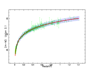
Figure 3: Hubble diagram for the Union 2.1 compilation , green points with error bar. The solid red line represents the best fit for the distance modulus in $\Lambda$CDM cosmology as represented by Eq. (11). The theoretical uncertainties are represented through blue vertical lines by applying the law of errors of Gauss with the uncertainties and parameters as in the first line of Table 1.

The second test we perform is on the the joint light-curve analysis (JLA), which contains 740 SNs [6] with data available on CDS at http://cdsweb.u-strasbg.fr/. The above compilation consists of SNe (type I-a) for which we have a heliocentric redshift, $z$, apparent magnitude $m_{B}^{\star}\,$ in the B band, error in $m_{B}^{\star}\,$, $\sigma_{m_{B}^{\star}\,}$, parameter $X1$, error in $X1$, $\sigma_{X1}$, parameter $C$, error in the parameter $C$, $\sigma_{C}$ and $\log_{10}(M_{stellar})$. The observed distance modulus is defined by Eq. (4) in [6]

$$m-M=-C\beta+{\it X1}\,\alpha-M_{{b}}+m_{B}^{\star}\,\quad.$$ (76)

The adopted parameters are $\alpha=0.141$, $\beta=3.101$ and

$$M_{{b}}=\begin{cases}-19.05&\text{if }M_{stellar}<10^{10}M_{\hbox{$\odot$}}\\ -19.12&\text{if }M_{stellar}\geq 10^{10}M_{\hbox{$\odot$}}\end{cases}\quad,$$ (77)

where $M_{\hbox{$\odot$}}$ is the mass of the sun, see line 1 in Table 10 of [6]. The uncertainty in the observed distance modulus, $\sigma_{m-M}$, is found by implementing the error propagation equation (often called the law of errors of Gauss) when the covariant terms are neglected, see equation (3.14) in [54],

$$\sigma_{m-M}=\sqrt{{\alpha}^{2}{\sigma_{{{\it X1}}}}^{2}+{\beta}^{2}{\sigma_{{C}}}^{2}+{\sigma_{{{\it m_{B}^{\star}\,}}}}^{2}}\quad.$$ (78)

The cosmological parameters with the JLA compilation are reported in see Table 2 and Figure 4 reports the best fit in the MTL cosmology.

Table 2: Numerical values of $\chi^{2}$, $\chi_{red}^{2}$, $Q$ and the AIC of the Hubble diagram for the JLA compilation, $k$ stands for the number of parameters, $H_{0}$ is expressed in $\mathrm{km\,s^{-1}\,Mpc^{-1}}$; 740 SNs.

cosmology	Eq.	$k$	parameters	$\chi 2$	$\chi_{red}^{2}$	$Q$	AIC
$\Lambda$CDM	(11)	3	$H_{0}=(70.71\pm 0.1)$; $\Omega_{\rm M}=(0.238\pm 0.01)$; $\Omega_{\Lambda}=(0.621\pm 0.01)$	626.53	0.85	0.998	632.53
wCDM	(23)	3	$H_{0}=(69.38\pm 0.31)$; $\Omega_{\rm M}=(0.2\pm 0.016)$ ; $w=(-0.8\pm 0.031)$	626.01	0.849	0.998	632.01
Cardassian	(31)	3	$H_{0}=(70.03\pm 0.44)$; $\Omega_{\rm M}=(0.3\pm 0.019)$ ; $n=(-0.055\pm 0.004)$	628.73	0.853	0.998	634.73
flat	(39)	2	$H_{0}=69.65\pm 0.23$; $\Omega_{\rm M}=0.3\pm 0.003$	627.91	0.85	0.998	631.91
$\phi$CDM	(46)	4	$H_{0}=69.6\pm 0.1$; $\Omega_{\rm M0}=0.24\pm 0.02$; $\alpha=0.31\pm 0.2$; $\beta=0.03\pm 0.02$	626.52	0.851	0.998	634.52
Einstein–De Sitter	(51)	1	$H_{0}=62.57\pm 0.17$	1307.75	1.76	$3.27\,10^{-34}$	1309.75
EdesNa	(52)	1	$H_{0}=68.91\pm 0.19$	630.46	0.853	0.998	632.46
simple GR	(60)	2	$H_{0}=73.79\pm 0.023$, $q_{0}$=-0.14	749.14	1.016	0.369	755.14
flat expanding model	(62)	1	$H_{0}=66.49\pm 0.18$	717.3	0.97	0.709	719.3
Milne	(64)	1	$H_{0}=67.19\pm 0.18$	656.11	0.887	0.986	658.11
plasma	(67)	1	$H_{0}=74.45\pm 0.2$	1017.79	1.377	3.59 $\,10^{-11}$	1019.79
MTL	(69)	2	$\beta$=2.36, $H_{0}=69.096\pm 0.32$	626.27	0.848	0.998	630.27

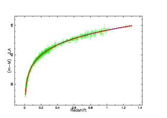
Figure 4: Hubble diagram for the JLA compilation, green points with error bar. The solid red line represents the best fit for the distance modulus in MTL cosmology as represented by Eq. (69). The theoretical uncertainties are represented through blue vertical lines.

The third test is performed on the Union 2.1 compilation (580 SNs) + the distance modulus for 59 calibrated high-redshift GRBs, the so called ‘Hymnium’ sample of GRBs, which allows to calibrate the distance modulus in the high redshift up to $z\approx 8$ [55], see Table 3 and Figure 5 for the best fit in the Cardassian cosmology.

Table 3: Numerical values of $\chi^{2}$, $\chi_{red}^{2}$, $Q$ and the AIC of the Hubble diagram for the Union 2.1 compilation + the ‘Hymnium’ GRB sample, $k$ stands for the number of parameters, $H_{0}$ is expressed in $\mathrm{km\,s^{-1}\,Mpc^{-1}}$; 580 SNs +59 GRBs.

cosmology	Eq.	$k$	parameters	$\chi 2$	$\chi_{red}^{2}$	$Q$	AIC
$\Lambda$CDM	(11)	3	$H_{0}=(67.8\pm 0.2)$ ; $\Omega_{\rm M}=(0.259\pm 0.02)$; $\Omega_{\Lambda}=(0.691\pm 0.02)$	586.04	0.921	0.922	592.04
wCDM	(23)	3	$H_{0}=(69.34\pm 0.32)$; $\Omega_{\rm M}=(0.2\pm 0.016)$ ; $w=(-0.626\pm 0.015)$	592.1	0.93	0.892	598.1
Cardassian	(31)	3	$H_{0}=(70.1\pm 0.42)$; $\Omega_{\rm M}=(0.299\pm 0.019)$ ; $n=(-0.063\pm 0.009)$	585.43	0.92	0.924	591.43
flat	(39)	2	$H_{0}=69.82\pm 0.24$; $\Omega_{\rm M}=0.295\pm 0.003$	585.74	0.919	0.927	589.74
$\phi$CDM	(46)	4	$H_{0}=70\pm 0.1$; $\Omega_{\rm M0}=0.28\pm 0.02$; $\alpha=-0.07\pm 0.2$; $\beta=0.05\pm 0.02$	585.41	0.922	0.92	593.41
Einstein–De Sitter	(51)	1	$H_{0}=63.14\pm 0.2$	1205.2	1.88	$3.58\,10^{-37}$	1205.21
EdesNa	(52)	1	$H_{0}=69.05\pm 0.22$	592.79	0.929	0.899	594.79
simple GR	(60)	2	$H_{0}=73.79\pm 0.023$, $q_{0}$=-0.01	809.5	1.27	$3.85\,10^{-6}$	813.5
flat expanding model	(62)	1	$H_{0}=66.851\pm 0.22$	676.36	1.06	0.141	678.36
Milne	(64)	1	$H_{0}=67.55\pm 0.22$	634.27	0.994	0.534	636.27
plasma	(67)	1	$H_{0}=74.25\pm 0.24$	951.16	1.49	9.39 $\,10^{-14}$	953.16
MTL	(69)	2	$\beta$=2.35 , $H_{0}=69.23\pm 0.34$	594.69	0.933	0.883	598.69

Figure 5: Hubble diagram for the Union 2.1 compilation + the ‘Hymnium’ GRB sample, green points with error bar. The solid red line represents the best fit for the distance modulus in Cardassian cosmology as represented by Eq. (31). The theoretical uncertainties are represented through blue vertical lines.

The fourth test is performed on the Pantheon sample of 1048 SN Ia [7, 8] with calibrated data available at https://archive.stsci.edu/prepds/ps1cosmo/jones_datatable.html, see Table 4 and Figure 6 for the best fit in the flat cosmology.

Table 4: Numerical values of $\chi^{2}$, $\chi_{red}^{2}$, $Q$ and the AIC of the Hubble diagram for the Pantheon sample, $k$ stands for the number of parameters, $H_{0}$ is expressed in $\mathrm{km\,s^{-1}\,Mpc^{-1}}$; 1048 SN Ia.

cosmology	Eq.	$k$	parameters	$\chi 2$	$\chi_{red}^{2}$	$Q$	AIC
$\Lambda$CDM	(11)	3	$H_{0}=(68.209\pm 0.2)$ ; $\Omega_{\rm M}=(0.278\pm 0.02)$; $\Omega_{\Lambda}=(0.651\pm 0.02)$	1054.71	1.01	0.41	1060.71
wCDM	(23)	3	$H_{0}=(69.8\pm 0.27)$; $\Omega_{\rm M}=(0.3\pm 0.016)$ ; $w=(-0.989\pm 0.03)$	1053.67	1	0.419	1059.67
Cardassian	(31)	3	$H_{0}=(70.01\pm 0.31)$; $\Omega_{\rm M}=(0.329\pm 0.014)$ ; $n=(-0.091\pm 0.005)$	1054.49	1	0.412	1060.49
flat	(39)	2	$H_{0}=69.94\pm 0.171$; $\Omega_{\rm M}=0.296\pm 0.002$	1053.53	1	0.429	1057.53
$\phi$CDM	(46)	4	$H_{0}=69.7\pm 0.1$; $\Omega_{\rm M0}=0.28\pm 0.02$; $\alpha=0.12\pm 0.2$; $\beta=0.05\pm 0.02$	1053.84	1	0.4	1061.84
Einstein–De Sitter	(51)	1	$H_{0}=62.71\pm 0.2$	2387.62	2.28	0	2389.62
EdesNa	(52)	1	$H_{0}=69.1\pm 0.13$	1059.84	1.01	0.384	1061.8
simple GR	(60)	2	$H_{0}=73.79\pm 0.015$, $q_{0}$=-0.063	1476.59	1.411	$2.67\,10^{-17}$	1480.59
flat expanding model	(62)	1	$H_{0}=66.67\pm 0.12$	1219	1.16	$1.6\,10^{-4}$	1221
Milne	(64)	1	$H_{0}=67.37\pm 0.12$	1132.6	1.08	0.033	1134.6
plasma	(67)	1	$H_{0}=74.7\pm 0.14$	2017.3	1.92	0	2019.3
MTL	(69)	2	$\beta$=2.31 , $H_{0}=68.95\pm 0.222$	1069.7	1.022	0.298	1073.7

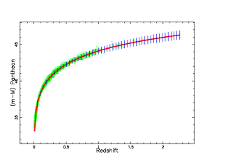
Figure 6: Hubble diagram for the Pantheon sample, green points with error bar. The solid red line represents the best fit for the distance modulus in flat cosmology as represented by Eq. (39). The theoretical uncertainties are represented through blue vertical lines.

In order to see how $\chi^{2}$ varies around the minimum for the Pantheon sample in the case of the $\Lambda$CDM cosmology, Figure 7 presents a 2D colour map for the values of $\chi^{2}$ for the Pantheon sample when $H_{0}$ and $\Omega_{\rm M}$ are allowed to vary around the numerical values which fix the minimum.

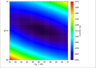
Figure 7: Color contour plot for $\chi 2$ of the Hubble diagram for the Pantheon sample in $\Lambda$CDM cosmology when $H_{0}$ and $\Omega_{\rm M}$ are variables and $\Omega_{\Lambda}=0.626$.

Figure 8 presents the map for $\chi^{2}$ for wCDM for the Pantheon sample when $H_{0}$ is fixed and $\Omega_{\rm M}$ and $w$ are allowed to vary.

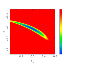
Figure 8: Map of $\chi^{2}$ for the wCDM cosmology when $H_{0}=69.8$.

3.4 Angular-diameter distance

In the relativistic models the angular diameter distance, $D_{\rm{A}}$ [56], is

$$D_{\rm{A}}=\frac{D_{\rm{L}}}{(1+z)^{2}}\quad.$$ (79)

We now introduce the minimax approximation. Let $f(x)$ be a real function defined in the interval $[a,b]$. The best rational approximation of degree $(k,l)$ evaluates the coefficients of the ratio of two polynomials of degree $k$ and $l$, respectively, which minimizes the maximum difference of

$$max\bigl{|}f(x)-\frac{p_{0}+p_{1}x+\dots+p_{k}x^{k}}{q_{0}+q_{1}x+\dots+q_{\ell}x^{\ell}}\bigr{|}\quad,$$ (80)

on the interval $[a,b]$. The quality of the fit is given by the maximum error over the considered range. The coefficients are evaluated through the Remez algorithm, see [57, 58]. The minimax approximation for the angular distance in the interval $0<z<8$ with data as in Table 3 for $\Lambda$CDM cosmology when $k=2$ and $p=2$ is

$$D_{A,2,2}={\frac{-0.08126207+\left(296.9974312+2.715947207\,z\right)z}{0.0672056121+\left(0.0810298760+0.02498056665\,z\right)z}}\,Mpc$$ (81)

$$maximum~{}error~{}=0.6911273~{}Mpc\quad,$$

for wCDM cosmology when $k=3$ and $p=2$ is

$$D_{A,3,2}=$$

$${\frac{0.034977336+\left(287.18685+\left(1.1871126+0.0002567152\,z\right)z\right)z}{0.0665238+\left(0.09134443+0.023282807\,z\right)z}}\,Mpc$$ (82)

$$maximum~{}error~{}=0.07~{}Mpc\quad,$$

for Cardassian cosmology when $k=2$ and $p=2$ is

$$D_{A,2,2}={\frac{-0.11928613+\left(273.3160492+2.420885784\,z\right)z}{0.0638700712+\left(0.0750594027+0.02611741351\,z\right)z}}\,Mpc$$ (83)

$$maximum~{}error~{}=0.8346776~{}Mpc\quad,$$

for flat cosmology when $k=2$ and $p=2$ is

$$D_{A,2,2}={\frac{-0.03653022+\left(274.6370918+2.192330157\,z\right)z}{0.0641307653+\left(0.0767316787+0.02582682170\,z\right)z}}Mpc$$ (84)

$$maximum~{}error~{}=0.629004~{}Mpc\quad,$$

and for $\phi$CDM cosmology when $k=2$ and $p=2$ is

$$D_{A,2,2}={\frac{-0.01852238+\left(278.5646306+2.230340777\,z\right)z}{0.0652823706+\left(0.0768568011+0.02575830541\,z\right)z}}$$ (85)

$$maximum~{}error~{}=0.6261293~{}Mpc\quad.$$

In MTL there is no difference between the distance $d$ , see equation (68), and the angular distance. We report the numerical value of $d$ in the interval $0<z<8$ with data as in Table 3

$$d=4330.383620\,\ln\left(z+1\right)\,Mpc\quad.$$ (86)

A promising field of investigation in applied cosmology is the maximum of the angular distance as function of the redshift [59, 60], $z_{max}$, which is finite in relativistic cosmologies and infinite in the Milne, plasma and MTL cosmologies, see Figure 9.

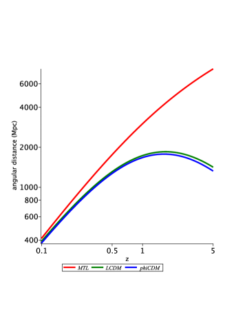
Figure 9: Angular distance in MTL (red) , $\Lambda$CDM (green) and $\phi$CDM (blue) cosmologies with data as in Table 3

The numerical value of $z_{max}$ is reported in Table 5, as a reference $z_{max}=1.594$ for flat Planck$\Lambda$CDM cosmology [61].

Table 5: Numerical values of $z_{max}$ and radius of Einstein ring in kpc when $R_{\mathrm{ave}}=1.54\,arcsec$

cosmology	$z_{max}$	radius (kpc)
$\Lambda$CDM	1.691	13.333
wCDM	1.716	11.797
Cardassian	1.607	11.938
flat	1.615	11.907
$\phi$CDM	1.632	12.05
MTL	$\infty$	45.15

Another example is given by the ring associated with the galaxy SDP.81, see [62], which is generally explained by the gravitational lens. In this framework we have a foreground galaxy at $z=0.2999$ and a background galaxy at $z=0.3042$. This ring has been studied with the Atacama Large Millimeter/sub-millimeter Array (ALMA) by [63, 64, 65, 66, 67, 68]. The system SDP.81 as been analysed by ALMA and presents 14 molecular clumps along the two main lensed arcs: the averaged radius in $arcsec$ is $R_{\mathrm{ave}}=1.54\,arcsec$ [69].

4 Conclusions

Cosmological models We list according to increasing order of the values of the merit function, $\chi^{2}$, the first, second, third and fourth cosmological models, see Table 6.

Table 6: The first, second, third and fourth best fitting models for the four compilations.

Compilation	first model	second model	third model	fourth model
Union 2.1	wCDM Hypergeometric	Cardassian	$\phi$CDM	flat
JLA	wCDM Hypergeometric	MTL	$\phi$CDM	$\Lambda$CDM
Union 2.1+GRBs	$\Lambda$CDM	$\phi$CDM	Cardassian	flat
Pantheon	wCDM Hypergeometric	Cardassian	flat	$\phi$CDM

The Einstein–De Sitter, simple GR and plasma models produce the highest values in the $\chi^{2}$ and are here considered only for historical reasons.

Physics versus Astronomy The value of the Newtonian gravitational constant, denoted by $G$, is derived applying the weighted mean, but the uncertainties were multiplied by a factor of 14, of 11 values available in Table XXIV in [70], see Figure 10.

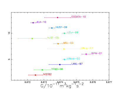
Figure 10: Values of the Newtonian constant of gravitation $G$ as given by Table XXIV in [70].

By analogy, we average the values of $H_{0}$ for the Pantheon sample and we report as error for $H_{0}$ the standard deviation

$$\overline{H_{0}}=(69.29\pm 3.18)\mathrm{km\,s^{-1}\,Mpc^{-1}}\quad Pantheon~{}sample\quad,$$ (87)

see Figure 11.

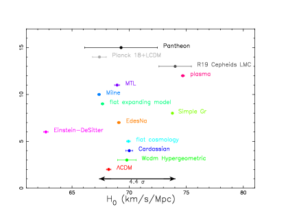
Figure 11: The present tension on $H_{0}$ (black line with two arrows) and our results in the case of the Pantheon sample with the connected averaged value which is marked as ‘Pantheon’; parameters as in Table 4.

Appendix A The Padé approximant

Given a function $f(z)$, the Padé approximant, after [71], is

$$f(z)=\frac{a_{0}+a_{1}z+\dots+a_{p}z^{p}}{b_{0}+b_{1}z+\dots+b_{q}z^{q}}\quad,$$ (A.1)

where the notation is the same as in [26].

The coefficients $a_{i}$ and $b_{i}$ are found through Wynn’s cross rule, see [72, 73] and our choice is $p=2$ and $q=2$. The choice of $p$ and $q$ is a compromise between precision (associated with high values for $p$ and $q$) and the simplicity of the expressions to manage (associated with low values for $p$ and $q$). The argument of the integral to be done is the inverse of $E(z)$, see Eq. (6),

$$\frac{1}{E(z)}=\frac{1}{\sqrt{\Omega_{\rm M}\,(1+z)^{3}+\Omega_{K}\,(1+z)^{2}+\Omega_{\Lambda}}}\quad,$$ (A.2)

and the Padé approximant is

$$\frac{1}{E(z)}=\frac{a_{0}+a_{1}z+a_{2}z^{2}}{b_{0}+b_{1}z+b_{2}z^{2}}\quad,$$ (A.3)

where

$$a_{0}=16\,\bigl{(}32\,{{\it\Omega_{K}}}^{3}{\it\Omega_{\Lambda}}+16\,{{\it\Omega_{K}}}^{2}{{\it\Omega_{\Lambda}}}^{2}+160\,{{\it\Omega_{K}}}^{2}{\it\Omega_{\Lambda}}\,{\it\Omega_{\rm M}}+24\,{{\it\Omega_{K}}}^{2}{{\it\Omega_{\rm M}}}^{2}$$

$$+64\,{\it\Omega_{K}}\,{{\it\Omega_{\Lambda}}}^{2}{\it\Omega_{\rm M}}+320\,{\it\Omega_{K}}\,{\it\Omega_{\Lambda}}\,{{\it\Omega_{\rm M}}}^{2}+40\,{\it\Omega_{K}}\,{{\it\Omega_{\rm M}}}^{3}+96\,{{\it\Omega_{\Lambda}}}^{2}{{\it\Omega_{\rm M}}}^{2}+$$

$$192\,{\it\Omega_{\Lambda}}\,{{\it\Omega_{\rm M}}}^{3}+15\,{{\it\Omega_{\rm M}}}^{4}\bigr{)}\bigl{(}{\it\Omega_{\rm M}}+{\it\Omega_{K}}+{\it\Omega_{\Lambda}}\bigr{)}^{4}$$ (A.4)

$$a_{1}=4\,\bigr{(}128\,{{\it\Omega_{K}}}^{4}{\it\Omega_{\Lambda}}+32\,{{\it\Omega_{K}}}^{3}{{\it\Omega_{\Lambda}}}^{2}+704\,{{\it\Omega_{K}}}^{3}{\it\Omega_{\Lambda}}\,{\it\Omega_{\rm M}}-16\,{{\it\Omega_{K}}}^{2}{{\it\Omega_{\Lambda}}}^{2}{\it\Omega_{\rm M}}$$

$$+1456\,{{\it\Omega_{K}}}^{2}{\it\Omega_{\Lambda}}\,{{\it\Omega_{\rm M}}}^{2}+32\,{{\it\Omega_{K}}}^{2}{{\it\Omega_{\rm M}}}^{3}-64\,{\it\Omega_{K}}\,{{\it\Omega_{\Lambda}}}^{3}{\it\Omega_{\rm M}}-384\,{\it\Omega_{K}}\,{{\it\Omega_{\Lambda}}}^{2}{{\it\Omega_{\rm M}}}^{2}$$

$$+1512\,{\it\Omega_{K}}\,{\it\Omega_{\Lambda}}\,{{\it\Omega_{\rm M}}}^{3}+50\,{\it\Omega_{K}}\,{{\it\Omega_{\rm M}}}^{4}-192\,{{\it\Omega_{\Lambda}}}^{3}{{\it\Omega_{\rm M}}}^{2}-288\,{{\it\Omega_{\Lambda}}}^{2}{{\it\Omega_{\rm M}}}^{3}$$

$$+648\,{\it\Omega_{\Lambda}}\,{{\it\Omega_{\rm M}}}^{4}+15\,{{\it\Omega_{\rm M}}}^{5}\bigr{)}\bigl{(}{\it\Omega_{\rm M}}+{\it\Omega_{K}}+{\it\Omega_{\Lambda}}\bigr{)}^{3}$$ (A.5)

$$a_{2}=-\bigl{(}256\,{{\it\Omega_{K}}}^{4}{\it\Omega_{\Lambda}}\,{\it\Omega_{\rm M}}-64\,{{\it\Omega_{K}}}^{3}{{\it\Omega_{\Lambda}}}^{3}+320\,{{\it\Omega_{K}}}^{3}{{\it\Omega_{\Lambda}}}^{2}{\it\Omega_{\rm M}}$$

$$+960\,{{\it\Omega_{K}}}^{3}{\it\Omega_{\Lambda}}\,{{\it\Omega_{\rm M}}}^{2}-320\,{{\it\Omega_{K}}}^{2}{{\it\Omega_{\Lambda}}}^{3}{\it\Omega_{\rm M}}+240\,{{\it\Omega_{K}}}^{2}{{\it\Omega_{\Lambda}}}^{2}{{\it\Omega_{\rm M}}}^{2}$$

$$+1440\,{{\it\Omega_{K}}}^{2}{\it\Omega_{\Lambda}}\,{{\it\Omega_{\rm M}}}^{3}+16\,{{\it\Omega_{K}}}^{2}{{\it\Omega_{\rm M}}}^{4}-1600\,{\it\Omega_{K}}\,{{\it\Omega_{\Lambda}}}^{3}{{\it\Omega_{\rm M}}}^{2}-480\,{\it\Omega_{K}}\,{{\it\Omega_{\Lambda}}}^{2}{{\it\Omega_{\rm M}}}^{3}$$

$$+1140\,{\it\Omega_{K}}\,{\it\Omega_{\Lambda}}\,{{\it\Omega_{\rm M}}}^{4}+20\,{\it\Omega_{K}}\,{{\it\Omega_{\rm M}}}^{5}-256\,{{\it\Omega_{\Lambda}}}^{4}{{\it\Omega_{\rm M}}}^{2}-1600\,{{\it\Omega_{\Lambda}}}^{3}{{\it\Omega_{\rm M}}}^{3}$$

$$-240\,{{\it\Omega_{\Lambda}}}^{2}{{\it\Omega_{\rm M}}}^{4}+380\,{\it\Omega_{\Lambda}}\,{{\it\Omega_{\rm M}}}^{5}+5\,{{\it\Omega_{\rm M}}}^{6}\bigr{)}\bigl{(}{\it\Omega_{\rm M}}+{\it\Omega_{K}}+{\it\Omega_{\Lambda}}\bigr{)}^{2}$$ (A.6)

$$b_{0}=16\,\bigl{(}{\it\Omega_{\rm M}}+{\it\Omega_{K}}+{\it\Omega_{\Lambda}}\bigr{)}^{9/2}\bigl{(}32\,{{\it\Omega_{K}}}^{3}{\it\Omega_{\Lambda}}+16\,{{\it\Omega_{K}}}^{2}{{\it\Omega_{\Lambda}}}^{2}+160\,{{\it\Omega_{K}}}^{2}{\it\Omega_{\Lambda}}\,{\it\Omega_{\rm M}}$$

$$+24\,{{\it\Omega_{K}}}^{2}{{\it\Omega_{\rm M}}}^{2}+64\,{\it\Omega_{K}}\,{{\it\Omega_{\Lambda}}}^{2}{\it\Omega_{\rm M}}+320\,{\it\Omega_{K}}\,{\it\Omega_{\Lambda}}\,{{\it\Omega_{\rm M}}}^{2}+40\,{\it\Omega_{K}}\,{{\it\Omega_{\rm M}}}^{3}$$

$$+96\,{{\it\Omega_{\Lambda}}}^{2}{{\it\Omega_{\rm M}}}^{2}+192\,{\it\Omega_{\Lambda}}\,{{\it\Omega_{\rm M}}}^{3}+15\,{{\it\Omega_{\rm M}}}^{4}\bigr{)}$$ (A.7)

$$b_{1}=4\,\bigl{(}{\it\Omega_{\rm M}}+{\it\Omega_{K}}+{\it\Omega_{\Lambda}}\bigr{)}^{7/2}\bigl{(}256\,{{\it\Omega_{K}}}^{4}{\it\Omega_{\Lambda}}+96\,{{\it\Omega_{K}}}^{3}{{\it\Omega_{\Lambda}}}^{2}+1536\,{{\it\Omega_{K}}}^{3}{\it\Omega_{\Lambda}}\,{\it\Omega_{\rm M}}$$

$$+96\,{{\it\Omega_{K}}}^{3}{{\it\Omega_{\rm M}}}^{2}+336\,{{\it\Omega_{K}}}^{2}{{\it\Omega_{\Lambda}}}^{2}{\it\Omega_{\rm M}}+3696\,{{\it\Omega_{K}}}^{2}{\it\Omega_{\Lambda}}\,{{\it\Omega_{\rm M}}}^{2}$$

$$+336\,{{\it\Omega_{K}}}^{2}{{\it\Omega_{\rm M}}}^{3}-64\,{\it\Omega_{K}}\,{{\it\Omega_{\Lambda}}}^{3}{\it\Omega_{\rm M}}+384\,{\it\Omega_{K}}\,{{\it\Omega_{\Lambda}}}^{2}{{\it\Omega_{\rm M}}}^{2}+4200\,{\it\Omega_{K}}\,{\it\Omega_{\Lambda}}\,{{\it\Omega_{\rm M}}}^{3}$$

$$+350\,{\it\Omega_{K}}\,{{\it\Omega_{\rm M}}}^{4}-192\,{{\it\Omega_{\Lambda}}}^{3}{{\it\Omega_{\rm M}}}^{2}+288\,{{\it\Omega_{\Lambda}}}^{2}{{\it\Omega_{\rm M}}}^{3}+1800\,{\it\Omega_{\Lambda}}\,{{\it\Omega_{\rm M}}}^{4}+105\,{{\it\Omega_{\rm M}}}^{5}\bigr{)}$$ (A.8)

$$b_{2}=\bigl{(}{\it\Omega_{\rm M}}+{\it\Omega_{K}}+{\it\Omega_{\Lambda}}\bigr{)}^{5/2}\bigl{(}512\,{{\it\Omega_{K}}}^{5}{\it\Omega_{\Lambda}}+384\,{{\it\Omega_{K}}}^{4}{{\it\Omega_{\Lambda}}}^{2}+3584\,{{\it\Omega_{K}}}^{4}{\it\Omega_{\Lambda}}\,{\it\Omega_{\rm M}}$$

$$+192\,{{\it\Omega_{K}}}^{3}{{\it\Omega_{\Lambda}}}^{3}+1984\,{{\it\Omega_{K}}}^{3}{{\it\Omega_{\Lambda}}}^{2}{\it\Omega_{\rm M}}+10752\,{{\it\Omega_{K}}}^{3}{\it\Omega_{\Lambda}}\,{{\it\Omega_{\rm M}}}^{2}+320\,{{\it\Omega_{K}}}^{3}{{\it\Omega_{\rm M}}}^{3}$$

$$+960\,{{\it\Omega_{K}}}^{2}{{\it\Omega_{\Lambda}}}^{3}{\it\Omega_{\rm M}}+5136\,{{\it\Omega_{K}}}^{2}{{\it\Omega_{\Lambda}}}^{2}{{\it\Omega_{\rm M}}}^{2}+17760\,{{\it\Omega_{K}}}^{2}{\it\Omega_{\Lambda}}\,{{\it\Omega_{\rm M}}}^{3}$$

$$+840\,{{\it\Omega_{K}}}^{2}{{\it\Omega_{\rm M}}}^{4}+2752\,{\it\Omega_{K}}\,{{\it\Omega_{\Lambda}}}^{3}{{\it\Omega_{\rm M}}}^{2}+7392\,{\it\Omega_{K}}\,{{\it\Omega_{\Lambda}}}^{2}{{\it\Omega_{\rm M}}}^{3}+$$

$$15060\,{\it\Omega_{K}}\,{\it\Omega_{\Lambda}}\,{{\it\Omega_{\rm M}}}^{4}$$

$$+700\,{\it\Omega_{K}}\,{{\it\Omega_{\rm M}}}^{5}+256\,{{\it\Omega_{\Lambda}}}^{4}{{\it\Omega_{\rm M}}}^{2}+2752\,{{\it\Omega_{\Lambda}}}^{3}{{\it\Omega_{\rm M}}}^{3}$$

$$+3696\,{{\it\Omega_{\Lambda}}}^{2}{{\it\Omega_{\rm M}}}^{4}+5020\,{\it\Omega_{\Lambda}}\,{{\it\Omega_{\rm M}}}^{5}+175\,{{\it\Omega_{\rm M}}}^{6}\bigr{)}.$$ (A.9)

The indefinite integral of (A.3), $F_{2,2}$, is

$$F_{2,2}(z;a_{0},a_{1},a_{2},b_{0},b_{1},b_{2})={\frac{a_{{2}}z}{b_{{2}}}}$$

$$+\frac{1}{2}\,{\frac{\ln\left({z}^{2}b_{{2}}+zb_{{1}}+b_{{0}}\right)a_{{1}}}{b_{{2}}}}-\frac{1}{2}\,{\frac{\ln\left({z}^{2}b_{{2}}+zb_{{1}}+b_{{0}}\right)a_{{2}}b_{{1}}}{{b_{{2}}}^{2}}}$$

$$+2\,{\frac{a_{{0}}}{\sqrt{4\,b_{{0}}b_{{2}}-{b_{{1}}}^{2}}}\arctan\left({\frac{2\,zb_{{2}}+b_{{1}}}{\sqrt{4\,b_{{0}}b_{{2}}-{b_{{1}}}^{2}}}}\right)}$$

$$-2\,{\frac{a_{{2}}b_{{0}}}{b_{{2}}\sqrt{4\,b_{{0}}b_{{2}}-{b_{{1}}}^{2}}}\arctan\left({\frac{2\,zb_{{2}}+b_{{1}}}{\sqrt{4\,b_{{0}}b_{{2}}-{b_{{1}}}^{2}}}}\right)}$$

$$-{\frac{b_{{1}}a_{{1}}}{b_{{2}}\sqrt{4\,b_{{0}}b_{{2}}-{b_{{1}}}^{2}}}\arctan\left({\frac{2\,zb_{{2}}+b_{{1}}}{\sqrt{4\,b_{{0}}b_{{2}}-{b_{{1}}}^{2}}}}\right)}$$

$$+{\frac{{b_{{1}}}^{2}a_{{2}}}{{b_{{2}}}^{2}\sqrt{4\,b_{{0}}b_{{2}}-{b_{{1}}}^{2}}}\arctan\left({\frac{2\,zb_{{2}}+b_{{1}}}{\sqrt{4\,b_{{0}}b_{{2}}-{b_{{1}}}^{2}}}}\right)}\quad.$$ (A.10)

References

• [1] Planck Collaboration, Aghanim N, Akrami Y and et al 2018 Planck 2018 results. VI. Cosmological parameters ArXiv e-prints (Preprint 1807.06209)
• [2] Riess A G, Casertano S, Yuan W, Macri L M and Scolnic D 2019 Large Magellanic Cloud Cepheid Standards Provide a 1% Foundation for the Determination of the Hubble Constant and Stronger Evidence for Physics beyond $\Lambda$CDM ApJ  876(1) 85 (Preprint 1903.07603)
• [3] Di Valentino E, Anchordoqui L A, Akarsu O and et al 2020 Cosmology Intertwined II: The Hubble Constant Tension arXiv e-prints arXiv:2008.11284 (Preprint 2008.11284)
• [4] Riess A G, Filippenko A V, Challis P and Clocchiatti A 1998 Observational Evidence from Supernovae for an Accelerating Universe and a Cosmological Constant AJ 116, 1009 (Preprint astro-ph/9805201)
• [5] Suzuki N, Rubin D, Lidman C, Aldering G, Amanullah R, Barbary K and Barrientos L F 2012 The Hubble Space Telescope Cluster Supernova Survey. V. Improving the Dark-energy Constraints above z greater than 1 and Building an Early-type-hosted Supernova Sample ApJ  746 85
• [6] Betoule M, Kessler R, Guy J and Mosher J 2014 Improved cosmological constraints from a joint analysis of the SDSS-II and SNLS supernova samples A&A  568 A22
• [7] Jones D O, Scolnic D M, Riess A G and et al 2018 Measuring Dark Energy Properties with Photometrically Classified Pan-STARRS Supernovae. II. Cosmological Parameters ApJ  857(1) 51 (Preprint 1710.00846)
• [8] Scolnic D M, Jones D O, Rest A and et al 2018 The Complete Light-curve Sample of Spectroscopically Confirmed SNe Ia from Pan-STARRS1 and Cosmological Constraints from the Combined Pantheon Sample ApJ  859(2) 101 (Preprint 1710.00845)
• [9] Oliveira F J 2016 Cosmic Time Transformations in Cosmological Relativity Journal of High Energy Physics, Gravitation and Cosmology 2, 253
• [10] Gupta R 2018 SNe Ia Redshift in a Nonadiabatic Universe Universe 4, 104 (Preprint 1810.12090)
• [11] Amarzguioui M, Elgarøy Ø, Mota D F and Multamäki T 2006 Cosmological constraints on f(R) gravity theories within the Palatini approach A&A  454(3), 707 (Preprint astro-ph/0510519)
• [12] Odintsov S D, Gómez D S C and Sharov G S 2019 Testing logarithmic corrections to R2-exponential gravity by observational data Phys. Rev. D 99(2) 024003
• [13] Corda C 2009 Interferometric Detection of Gravitational Waves: . the Definitive Test for General Relativity International Journal of Modern Physics D 18(14), 2275 (Preprint 0905.2502)
• [14] Lin H N, Li X and Tang L 2019 Non-parametric reconstruction of dark energy and cosmic expansion from the Pantheon compilation of type Ia supernovae Chinese Physics C 43(7) 075101 (Preprint 1905.11593)
• [15] Camlıbel A K, Semiz I and Feyizoğlu M 2020 Pantheon update on a model-independent analysis of cosmological supernova data arXiv preprint arXiv:2001.04408
• [16] Hogg D W 1999 Distance measures in cosmology ArXiv Astrophysics e-prints (Preprint astro-ph/9905116)
• [17] Peebles P J E 1993 Principles of Physical Cosmology (Princeton, N.J.: Princeton University Press)
• [18] Zaninetti L 2016 Pade approximant and minimax rational approximation in standard cosmology Galaxies 4(1), 4 ISSN 2075-4434 URL http://www.mdpi.com/2075-4434/4/1/4
• [19] Turner M S and White M 1997 CDM models with a smooth component Phys. Rev. D 56(8), R4439 (Preprint astro-ph/9701138)
• [20] Tripathi A, Sangwan A and Jassal H K 2017 Dark energy equation of state parameter and its evolution at low redshift Journal of Cosmology and Astroparticle Physic 6 012 (Preprint 1611.01899)
• [21] Wei J J, Ma Q B and Wu X F 2015 Utilizing the Updated Gamma-Ray Bursts and Type Ia Supernovae to Constrain the Cardassian Expansion Model and Dark Energy Advances in Astronomy 2015 576093 (Preprint 1504.02308)
• [22] Abramowitz M and Stegun I A 1965 Handbook of Mathematical Functions with Formulas, Graphs, and Mathematical Tables (New York: Dover)
• [23] von Seggern D 1992 CRC Standard Curves and Surfaces (New York: CRC)
• [24] Thompson W J 1997 Atlas for computing mathematical functions (New York: Wiley-Interscience)
• [25] Gradshteyn, I S and Ryzhik, I M and Jeffrey, A and Zwillinger, D 2007 Table of Integrals, Series, and Products (New York: Academic Press)
• [26] Olver F W J, Lozier D W, Boisvert R F and Clark C W 2010 NIST Handbook of Mathematical Functions (Cambridge: Cambridge University Press. )
• [27] Zaninetti L 2019 The Distance Modulus in Dark Energy and Cardassian Cosmologies via the Hypergeometric Function International Journal of Astronomy and Astrophysics 9(3), 231 (Preprint 1909.02360)
• [28] Freese K and Lewis M 2002 Cardassian expansion: a model in which the universe is flat, matter dominated, and accelerating Physics Letters B 540, 1 (Preprint astro-ph/0201229)
• [29] Freese K 2003 Generalized cardassian expansion: a model in which the universe is flat, matter dominated, and accelerating Nuclear Physics B Proceedings Supplements 124, 50 (Preprint hep-ph/0208264)
• [30] Baes M, Camps P and Van De Putte D 2017 Analytical expressions and numerical evaluation of the luminosity distance in a flat cosmology MNRAS  468, 927 (Preprint 1702.08860)
• [31] Zaninetti L 2019 A New Analytical Solution for the Distance Modulus in Flat Cosmology International Journal of Astronomy and Astrophysics 9(1), 51 (Preprint 1903.07121)
• [32] Starobinsky A A 1980 A new type of isotropic cosmological models without singularity Physics Letters B 91(1), 99
• [33] Guth A H and Weinberg E J 1981 Cosmological consequences of a first-order phase transition in the SU5 grand unified model Phys. Rev. D 23(4), 876
• [34] Ratra B and Peebles P J E 1988 Cosmological consequences of a rolling homogeneous scalar field Phys. Rev. D 37(12), 3406
• [35] Steinhardt P J and Caldwell R R 1998 Introduction to Quintessence in Y I Byun and K W Ng, eds, Cosmic Microwave Background and Large Scale Structure of the Universe vol 151 of Astronomical Society of the Pacific Conference Series p 13
• [36] Avsajanishvili O, Huang Y, Samushia L and Kahniashvili T 2018 The observational constraints on the flat $\varphi$ CDM models European Physical Journal C 78(9) 773 (Preprint %****␣ms.tex␣Line␣2450␣****1711.11465)
• [37] Mamon A A, Bamba K and Das S 2017 Constraints on reconstructed dark energy model from SN Ia and BAO/CMB observations European Physical Journal C 77(1) 29 (Preprint 1607.06631)
• [38] Einstein A and de Sitter W 1932 On the Relation between the Expansion and the Mean Density of the Universe Proceedings of the National Academy of Science 18, 213
• [39] Krisciunas K 1993 Look-Back Time the Age of the Universe and the Case for a Positive Cosmological Constant JRASC 87, 223 (Preprint astro-ph/9306002)
• [40] Ryden B 2003 Introduction to Cosmology (San Francisco, CA, USA: Addison Wesley)
• [41] Lang K 2013 Astrophysical Formulae: Space, Time, Matter and Cosmology Astronomy and Astrophysics Library (Berlin: Springer) ISBN 9783662216392
• [42] Heymann Y 2013 On the luminosity distance and the hubble constant Progress in Physics 3, 5
• [43] Milne E A 1933 World-Structure and the Expansion of the Universe. Zeitschrift fur Astrophysik 6, 1
• [44] Chodorowski M J 2005 Cosmology Under Milne’s Shadow PASA 22, 287 (Preprint astro-ph/0503690)
• [45] Adamek J, Di Dio E, Durrer R and Kunz M 2014 Distance-redshift relation in plane symmetric universes Phys. Rev. D 89(6) 063543 (Preprint 1401.3634)
• [46] Brynjolfsson A 2004 Redshift of photons penetrating a hot plasma arXiv:astro-ph/0401420
• [47] Brynjolfsson A 2006 Magnitude-Redshift Relation for SNe Ia, Time Dilation, and Plasma Redshift ArXiv:astro-ph/0602500
• [48] Marmet L 2018 On the Interpretation of Spectral Red-Shift in Astrophysics: A Survey of Red-Shift Mechanisms - II arXiv e-prints arXiv:1801.07582 (Preprint 1801.07582)
• [49] Zaninetti L 2015 On the Number of Galaxies at High Redshift Galaxies 3, 129
• [50] Press W H, Teukolsky S A, Vetterling W T and Flannery B P 1992 Numerical Recipes in FORTRAN. The Art of Scientific Computing (Cambridge, UK: Cambridge University Press)
• [51] Akaike H 1974 A new look at the statistical model identification IEEE Transactions on Automatic Control 19, 716
• [52] Liddle A R 2004 How many cosmological parameters? MNRAS  351, L49
• [53] Godlowski W and Szydowski M 2005 Constraints on Dark Energy Models from Supernovae in M Turatto, S Benetti, L Zampieri and W Shea, eds, 1604-2004: Supernovae as Cosmological Lighthouses (Astronomical Society of the Pacific) vol 342 of Astronomical Society of the Pacific Conference Series pp 508–516
• [54] Bevington, P R and Robinson, D K 2003 Data Reduction and Error Analysis for the Physical Sciences (New York: McGraw-Hill)
• [55] Wei H 2010 Observational constraints on cosmological models with the updated long gamma-ray bursts Journal of Cosmology and Astroparticle Physic 8 020 (Preprint 1004.4951)
• [56] Etherington I M H 1933 On the Definition of Distance in General Relativity. Philosophical Magazine 15
• [57] Remez E 1934 Sur la détermination des polynômes d´approximation de degré donnée Comm. Soc. Math. Kharkov 10, 41
• [58] Remez E 1957 General Computation Methods of Chebyshev Approximation. The Problems with Linear Real Parameters (Kiev: Publishing House of the Academy of Science of the Ukrainian SSR)
• [59] Braatz J A, Reid M J, Humphreys E M L, Henkel C, Condon J J and Lo K Y 2010 The Megamaser Cosmology Project. II. The Angular-diameter Distance to UGC 3789 ApJ  718(2), 657 (Preprint 1005.1955)
• [60] Kuo C Y, Braatz J A, Reid M J, Lo K Y, Condon J J, Impellizzeri C M V and Henkel C 2013 The Megamaser Cosmology Project. V. An Angular-diameter Distance to NGC 6264 at 140 Mpc ApJ  767(2) 155 (Preprint 1207.7273)
• [61] Melia F and Yennapureddy M K 2018 The maximum angular-diameter distance in cosmology MNRAS  480(2), 2144 (Preprint 1807.07548)
• [62] Eales S, Dunne L, Clements D and Cooray A 2010 The Herschel ATLAS PASP 122, 499 (Preprint 0910.4279)
• [63] Tamura Y, Oguri M, Iono D, Hatsukade B, Matsuda Y and Hayashi M 2015 High-resolution ALMA observations of SDP.81. I. The innermost mass profile of the lensing elliptical galaxy probed by 30 milli-arcsecond images PASJ  67 72 (Preprint 1503.07605)
• [64] ALMA Partnership, Vlahakis C, Hunter T R and Hodge J A 2015 The 2014 ALMA Long Baseline Campaign: Observations of the Strongly Lensed Submillimeter Galaxy HATLAS J090311.6+003906 at z = 3.042 ApJ Letters, 808 L4 (Preprint 1503.02652)
• [65] Rybak M, Vegetti S, McKean J P, Andreani P and White S D M 2015 ALMA imaging of SDP.81 - II. A pixelated reconstruction of the CO emission lines MNRAS  453, L26 (Preprint 1506.01425)
• [66] Hatsukade B, Tamura Y, Iono D, Matsuda Y, Hayashi M and Oguri M 2015 High-resolution ALMA observations of SDP.81. II. Molecular clump properties of a lensed submillimeter galaxy at z = 3.042 PASJ  67 93 (Preprint 1503.07997)
• [67] Wong K C, Suyu S H and Matsushita S 2015 The Innermost Mass Distribution of the Gravitational Lens SDP.81 from ALMA Observations ApJ  811 115 (Preprint 1503.05558)
• [68] Hezaveh Y D, Dalal N and Marrone D P 2016 Detection of Lensing Substructure Using ALMA Observations of the Dusty Galaxy SDP.81 ApJ  823 37 (Preprint 1601.01388)
• [69] Zaninetti L 2017 The ring produced by an extra-galactic superbubble in flat cosmology Journal of High Energy Physics, Gravitation and Cosmology 3, 339
• [70] Mohr P J, Taylor B N and Newell D B 2012 CODATA recommended values of the fundamental physical constants: 2010 Reviews of Modern Physics 84, 1527
• [71] Padé H 1892 Sur la représentation approchée d’une fonction par des fractions rationnelles Ann. Sci. Ecole Norm. Sup. 9, 193
• [72] Baker G 1975 Essentials of Padé approximants (New York: Academic Press)
• [73] Baker G A and Graves-Morris P R 1996 Padé approximants vol 59 (Cambridge: Cambridge University Press)