Reconstruction of photon number conditioned states using phase randomised homodyne measurements

Abstract

We experimentally demonstrate the reconstruction of a photon number conditioned state without using a photon number discriminating detector. By using only phase randomised homodyne measurements, we reconstruct up to the three photon subtracted squeezed vacuum state. The reconstructed Wigner functions of these states show regions of pronounced negativity, signifying the non-classical nature of the reconstructed states. The techniques presented allow for complete characterisation of the role of a conditional measurement on an ensemble of states, and might prove useful in systems where photon counting is still technically challenging.

1 Introduction

Central to the weirdness of quantum mechanics is the notion of wave-particle duality, where classical concepts of particle or wave behaviour alone cannot provide a complete description of quantum objects. When investigating quantum systems, information concerning one description is typically sacrificed in favour of the other, depending on which description suits your endeavour. Probing the continuous variables of an infinite Hilbert space, such as the amplitude and phase of a light field, is often viewed as less interesting than probing the quantised variables of a quantum system. This is largely due to the fact that, given current technology, when probing the continuous variables (CV) of a quantum system alone, one is restricted to transformations that map Gaussian states onto Gaussian states. Nevertheless, the idea of measuring the quantised nature of light with only CV techniques has been theoretically [1, 2, 3, 4] and experimentally [5, 6, 7, 8] investigated.

The usual CV toolbox of Gaussian transformations, comprising beam splitters, displacements, rotations, squeezing, homodyne and heterodyne detection allows for deterministic manipulation of quantum optical states that can be experimentally realised with typically very high efficiency. However, the absence of a strong non-linearity within this toolbox severely handicaps the reach of CV techniques for quantum information processing applications [9, 10]. Conversely, DV is implicitly non-linear—forgoing determinism to harness the measurement-induced non-linearity of a photon-counting measurement. Recently, there has been a move to hybridise both CV and DV techniques for quantum information purposes, as one non-Gaussian operation, when combined with Gaussian resources and operations, is sufficient to realise universal quantum computing [11].

Here we present the CV analog of the photon counting measurement, whereby we replace a non-deterministic photon counting measurement with a deterministic phase randomised measurement of the field quadratures. This extends the ideas reported in [4, 12] to show how the requirement of a photon counting measurement can be replaced by CV measurements for the reconstruction of the statistics of non-Gaussian states. This approach forgoes the shot by shot nature of DV photon counting in favour of ensemble measurements, and consequently cannot be appropriated for state preparation. As we only preform Gaussian measurements, all the directly measured statistics remain Gaussian and the ‘non-Gaussianity’ emerges in the nature of post-processing preformed. The inherently ensemble nature of the technique and our restriction to Gaussian measurements ensure it can never be used to prepare a non-Gaussian state—in accordance with the limitations of Gaussian toolbox. It does, however, still permit access to the same non-Gaussian statistics that were previously only accessible with the requirement of a projective photon counting measurement. Using this method, we have successfully reconstructed the non-Gaussian 1, 2 and 3 photon subtracted squeezed vacuum (PSSV) states.

The context for the implementation of this protocol will be the characterisation of the PSSV states. Also coined ‘kitten states’, due to their high fidelity with small amplitude Schrödinger cat states, these states are typically prepared by annihilating one or more photons from a squeezed vacuum state [13]. This ‘annihilation’ is experimentally realised to high fidelity with a beam splitter of weak reflectivity and a conditional photon counting measurement, such that the detection of a photon in the reflected mode heralds the successful subtraction of a photon. Interest in such states was mainly prompted by optical quantum computing [14, 15], but they are also of interest for metrology and entanglement distillation [16, 17]. Experiments involving the generation of kitten states were amongst the first hybridisation experiments—bridging the gap between two historically distinct areas of quantum optics [18, 19, 20, 21, 22].

This paper is organised as follows: in Section 2, we discuss the theory linking homodyne detection and photon counting measurement. Section 3 discusses the experimental implementation. We present the experimental results in Section 4. The Appendix provides the conditioning functions that transform photon counting measurements to homodyne observables.

2 Theory

We want to design the homodyne equivalent of a heralded photon discriminating measurement. The setup consist of a correlated two mode state $\rho_{ab}$, where mode $a$ is used to condition the outcome of mode $b$ (see Figure 2). The conditioning measurement consists of sampling the homodyne observable $\hat{X}_{a}^{\phi}$ in a phase randomised manner such that each quadrature angle, $\phi$ contributes equally. Here, $\hat{X}^{\phi}_{a}=e^{-i\phi}\hat{a}_{a}+e^{i\phi}\hat{a}_{a}^{\dagger}$, where $\hat{a}_{a}$ and $\hat{a}_{a}^{\dagger}$ are the annihilation and creation operators in mode $a$ and $\phi$ is the field quadrature angle. The conditioned mode $b$ is then characterised via homodyne tomography.

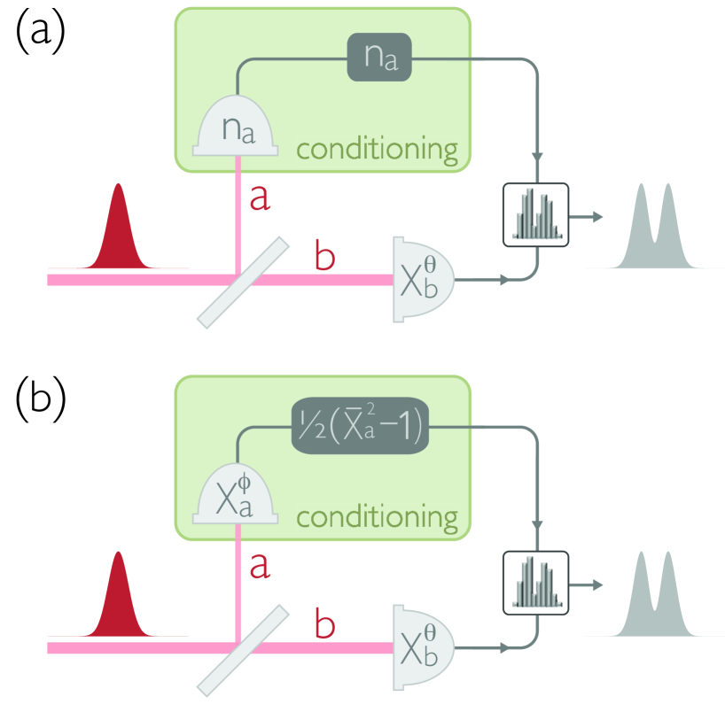
Figure 1: (a) A photon number discriminating detector heralds a successful preparation. The correctly prepared state is subsequently reconstructed via homodyne tomography. (b) The same statistics of the state heralded by a photon counting measurement can be retrieved by replacing the photon number discriminating detector with a phase randomised homodyne detection and appropriate post-processing.

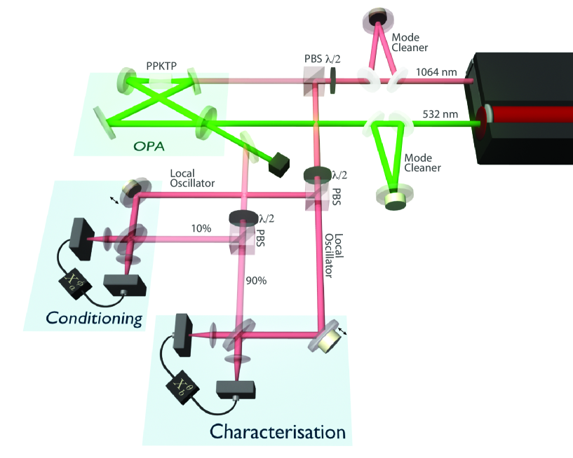
Figure 2: Experimental Setup A CW Nd:YAG laser at 1064 nm provides the laser resource for this experiment. An internal second harmonic generation (SHG) cavity frequency doubles a portion of the 1064nm light. Both the 1064 nm and 532 nm fields undergo spatial and frequency filtering before providing seed and pump resources respectively for a doubly-resonant optical parametric amplifier (OPA). A small portion of the resulting squeezed coherent state is then reflected for ’conditioning’ by a variable beam-splitter - implement with a $\lambda/2$ wave-plate and a polarising beam splitter (PBS). The reflected light (mode $a$) is subsequently sampled via a phase randomised homodyne detection. The remaining transmitted light (mode $b$) is characterised by a tomographic homodyne detection, sampling $X^{\theta}_{b}$ for $\theta=0\ldots 165^{\circ}$ in intervals of $15^{\circ}$.

If $\rho_{ab}$ originates from a squeezed vacuum mode passing through a weakly reflecting beam splitter, the resulting mode at $b$ conditioned on finding $n$ photons at $a$ will be an $n$-PSSV state.

We demonstrate how this conditioning can be performed using two approaches. In the first approach, we express a polynomial operator function of $\hat{n}_{a}$ that we want to condition upon in terms of homodyne observables $\hat{X}^{\phi}_{a}$. In the second approach, we utilise the pattern functions [1] to access an inner product in the Fock basis via homodyne measurements.

2.1 Transformation Polynomials

In this section, our goal is to obtain the measurement statistics that would correspond to measuring a two mode observable $F(\hat{n}_{a})\otimes G(\hat{b})$ without actually constructing a device that directly detects $F(\hat{n}_{a})$. Instead we will be measuring quadrature values of $a$. As we shall see in the following subsections, by suitably conditioning on a homodyne measurement outcome of $a$, one can recover the statistics of an $m$-photon subtracted state at $b$.

Example 1: Conditioning on $\hat{n}_{a}$.

In the first example, we will attempt to condition the output state $b$ on the measurement outcome of operator $\hat{n}_{a}$. We want to estimate the expectation value

$$g\left(X_{b}^{\theta}\right)=\textrm{tr}\left\{\rho_{ab}\;\hat{n}_{a}\otimes\left|{X_{b}^{\theta}}\right\rangle\left\langle{X_{b}^{\theta}}\right|\right\}\;,$$ (1)

where $\rho_{ab}$ is the joint state at modes $a$ and $b$. Expanding the operator $\hat{n}_{a}$, $g\left(X_{b}^{\theta}\right)$ can be written as

$$g\left(X_{b}^{\theta}\right) =\sum_{n}n\,\mathrm{pr}(n)\textrm{tr}\left\{\rho_{b}(n)\left|{X_{b}^{\theta}}\right\rangle\left\langle{X_{b}^{\theta}}\right|\right\}$$ (2)

$$=\sum_{n}n\,\mathrm{pr}(n)\,\mathrm{pr}(X_{b}^{\theta}|n)$$ (3)

$$=\sum_{n}n\,\mathrm{pr}(X_{b}^{\theta},n)\;.$$ (4)

We use $\mathrm{pr}$ to denote probabilities and $\mathrm{pr}(n)$ denotes the probability of getting an outcome $n$ at $a$. $\rho_{b}(n)$ is the state at $b$ conditioned on an outcome $n$ at $a$.

In particular, we consider $\rho_{ab}$ is a weakly squeezed vacuum state passing through a low reflectivity beam-splitter with vacuum entering through the other input. Ignoring higher order terms, a squeezed state can be approximated by $\left|{\psi}\right\rangle=\left|{0}\right\rangle-\left|{2}\right\rangle\gamma$ where $\gamma\ll 1$. $\left|{n}\right\rangle$ is the Fock state with $n$ photons. The beam-splitter transforms this state to

$$\left|{0,0}\right\rangle+\left(\left|{1,1}\right\rangle\sqrt{2\eta^{2}(1-\eta^{2})}+\left|{2,0}\right\rangle(1-\eta^{2})+\left|{0,2}\right\rangle\eta^{2}\right)\gamma$$ (5)

where the beam splitter transmissivity is $\eta\sim 1$. $\left|{n,m}\right\rangle$ is the Fock state with $n$ photons in the first output (mode $a$) and $m$ photons in the second output (mode $b$).

For this state, the expectation value, equation (1) becomes

$$\textrm{tr}\left\{\left(\left|{1}\right\rangle\left\langle{1}\right|2\eta^{2}(1-\eta^{2})+\left|{0}\right\rangle\left\langle{0}\right|2(1-\eta^{2})^{2}\right)\left|{X_{b}^{\theta}}\right\rangle\left\langle{X_{b}^{\theta}}\right|\right\}\gamma^{2}\;,$$ (6)

where the second term arises from the probability of reflecting two photons. Assuming this probability is small (for $\eta\sim 1$), the output expectation value gives the statistics corresponding to a single photon Fock state.

To realise this conditioning, we could measure $a$ in the Fock basis $\left|{n}\right\rangle\left\langle{n}\right|$ and scale the measurement outcomes of $b$ by the outcomes $n_{a}$ (see Figure 1 (a)). But suppose we are restricted to only homodyne tomography. We can still realise the conditioning by expressing $\hat{n}$ in terms the quadrature operators $\hat{X}$ and $\hat{P}$:

$$\hat{n}=\frac{1}{4}\left(\hat{X}^{2}+\hat{P}^{2}-2\right)\;$$ (7)

where $\hat{X}$ and $\hat{P}$ are two orthogonal quadrature operators with the commutation relation $[\hat{X},\hat{P}]=2i$. Although $\hat{X}$ and $\hat{P}$ cannot be measured simultaneously, Equation (1) can nevertheless can be written as the sum

$$g\left(X_{b}^{\theta}\right) =\textrm{tr}\left\{\rho_{ab}\;\frac{1}{4}(\hat{X}^{2}-1)\otimes\left|{X_{b}^{\theta}}\right\rangle\left\langle{X_{b}^{\theta}}\right|\right\}$$ (8)

$$+\textrm{tr}\left\{\rho_{ab}\;\frac{1}{4}(\hat{P}^{2}-1)\otimes\left|{X_{b}^{\theta}}\right\rangle\left\langle{X_{b}^{\theta}}\right|\right\}\;.$$ (9)

The expectation value $g\left(X_{b}^{\theta}\right)$ can be built up by combining the outcomes of two independent measurements.

Phase randomised measurements: The quadratures $\hat{X}$ and $\hat{P}$ can be replaced by any pair of orthogonal quadratures. Instead of locking the quadrature angles, we can also randomise the phase by scanning the local oscillator. Equation (7) can be written as an integration over all phases

$$\hat{n} =\frac{1}{2\pi}\int_{0}^{2\pi}\frac{1}{4}\left[(\hat{X}^{\phi})^{2}+(\hat{X}^{\phi+\frac{\pi}{2}})^{2}-2\right]d\phi$$ (10)

$$=\frac{1}{2}\left(\bar{X}^{2}-1\right)\;,$$ (11)

where

$$\bar{X}^{n}=\frac{1}{2\pi}\int_{0}^{2\pi}(\hat{X}^{\phi})^{n}d\phi$$ (12)

is the phase averaged quadrature moment operator. Substituting this into Equation (1) we obtain

$$g\left(X_{b}^{\theta}\right)=\textrm{tr}\left\{\rho_{ab}\;\frac{1}{2}\left(\bar{X}_{a}^{2}-1\right)\otimes\left|{X_{b}^{\theta}}\right\rangle\left\langle{X_{b}^{\theta}}\right|\right\}\;.$$ (13)

So $g\left(X_{b}^{\theta}\right)$ can be obtained by a phase randomised sampling of the quadratures and weighting the outcomes at $b$ by the outcomes of $\frac{1}{2}(\bar{X}_{a}^{2}-1)$ at $a$ (Figure 1b).

Example 2: Conditioning on $\hat{n}_{a}(\hat{n}_{a}-2)$.

To obtain a more faithful reproduction of the single photon Fock state distributions from a weakly squeezed state, we can weight the outcomes on $\hat{n}_{a}(\hat{n}_{a}-2)$ instead. This removes the contribution of two photon states at mode $a$. For a weakly squeezed vacuum input state (neglecting four photon terms), the analogue of Equation (6) for this conditioning is

$$g\left(X_{b}^{\theta}\right)=\textrm{tr}\left\{\left|{1}\right\rangle\left\langle{1}\right|2\eta^{2}(1-\eta^{2})\left|{X_{b}^{\theta}}\right\rangle\left\langle{X_{b}^{\theta}}\right|\right\}\gamma^{2}\;.$$ (14)

To achieve this conditioning via homodyne measurements, we repeat the recipe as before to express $\hat{n}$ in terms quadrature variables $\hat{X}$ and $\hat{P}$:

$$\hat{n}(\hat{n}-2) =\frac{1}{16}\left(\hat{X}^{2}+\hat{P}^{2}-2\right)\left(\hat{X}^{2}+\hat{P}^{2}-10\right)$$ (15)

$$=\frac{1}{16}\left(2\bar{X}^{4}-24\bar{X}^{2}+20+\hat{X}^{2}\hat{P}^{2}+\hat{P}^{2}\hat{X}^{2}\right)\;.$$ (16)

The terms involving products of $\hat{X}$ and $\hat{P}$ cannot be evaluated directly through a phase randomised homodyne measurement. In order to make them accessible, we need to express $\hat{X}^{2}\hat{P}^{2}+\hat{P}^{2}\hat{X}^{2}$ as a function of $\bar{X}$ which can be done as follows:

$$\hat{X}^{2}\hat{P}^{2}+\hat{P}^{2}\hat{X}^{2}=\frac{1}{2\pi}\int_{0}^{2\pi}2(\hat{X}^{\phi})^{2}(\hat{X}^{\phi+\frac{\pi}{2}})^{2}d\phi$$ (17)

$$=\frac{1}{\pi}\int_{0}^{2\pi}(2\hat{a}_{\phi}^{\dagger}\hat{a}_{\phi}\hat{a}_{\phi}^{\dagger}\hat{a}_{\phi}+2\hat{a}_{\phi}^{\dagger}\hat{a}_{\phi}-1-\hat{a}_{\phi}^{4}-(\hat{a}_{\phi}^{\dagger})^{4})d\phi$$ (18)

$$=\frac{1}{\pi}\int_{0}^{2\pi}(2\hat{a}_{\phi}^{\dagger}\hat{a}_{\phi}\hat{a}_{\phi}^{\dagger}\hat{a}_{\phi}+2\hat{a}_{\phi}^{\dagger}\hat{a}_{\phi}-1)d\phi$$ (19)

$$=\frac{1}{\pi}\int_{0}^{2\pi}\left(\frac{(\hat{a}_{\phi}^{\dagger}+\hat{a}_{\phi})^{4}}{3}-2\right)d\phi$$ (20)

$$=\frac{2\bar{X}^{4}}{3}-4\;,$$ (21)

where we define $\hat{a}_{\phi}=\hat{a}\exp(-i\phi)$. Substituting this into Equation (16), we obtain the sampling polynomial as

$$\hat{n}(\hat{n}-2)=\frac{\bar{X}^{4}}{6}-\frac{3\bar{X}^{2}}{2}+1\;.$$ (22)

With this, the expectation value becomes

$$g\left(X_{b}^{\theta}\right)=\textrm{tr}\left\{\rho_{ab}\left(\frac{\bar{X}_{a}^{4}}{6}-\frac{3\bar{X}_{a}^{2}}{2}+1\right)\otimes\left|{X_{b}^{\theta}}\right\rangle\left\langle{X_{b}^{\theta}}\right|\right\}\;$$ (23)

which can be sampled via a randomised phase quadrature measurement.

General conditioning on $f(\hat{n}_{a})$.

Higher order polynomials of $\hat{n}$ can be constructed in a similar way. We provide two algorithms in Appendix A. These polynomials provide a simple construction for a $k$ photon subtracted state by conditioning on

$$\mathcal{P}(\hat{n})=\frac{1}{\hat{n}-k}\prod_{j=0}^{j_{max}}\hat{n}-j\;$$ (24)

with $j_{max}>k$. Increasing $j_{max}$ in the product above would correct for higher photon number contributions up to $j_{max}$. But this will be at the expense of a higher weighting from outcomes having photon numbers greater than $j_{max}$. If the probabilities of these outcomes are large, it could dilute the actual conditioning state that we are interested in.

As an example, to get a two photon subtracted state, we can use the conditioning polynomial with $k=2$ and $j_{max}=6$:

$$\mathcal{P}(\hat{n})=\hat{n}(\hat{n}-1)(\hat{n}-3)(\hat{n}-4)(\hat{n}-5)\;.$$ (25)

Expanding in the Fock basis,

$$\mathcal{P}(\hat{n})=-12\left|{2}\right\rangle\left\langle{2}\right|+180\left|{7}\right\rangle\left\langle{7}\right|+1008\left|{8}\right\rangle\left\langle{8}\right|+\ldots$$ (26)

In this example, we see that the seven and eight photons events are weighted by a factor of 15 and 84 compared to the two photon events. In most applications however, these high photon number states would have exponentially vanishing probabilities.

2.2 Pattern functions

The pattern functions, first introduced in [1, 23], specify the link between homodyne observables of a quantum state and the density matrix. These set of sampling functions allow reconstruction of the density matrix without the requirement of first reconstructing the Wigner function.

We want to characterise the state at $a$ conditioned on an $n$ photon event at $b$. Ideally, we would choose an appropriate polynomial in $X_{a}^{\phi}$ that corresponds to $\left|{n}\right\rangle\left\langle{n}\right|$. Practically, however, we can only realise a polynomial of a limited order—correcting for the finite undesired photon number events that may prove statistically significant. The pattern functions however permit a perfectly isolating characterisation that removes all unwanted photon number events.

We start with the general problem of reconstructing the statistics of the post-selected state at $b$, $\tilde{\rho}_{b}$, conditioned on the event of having a state $\rho_{a}^{cond}$ at $a$. This conditioning can be achieved by means of a measurement apparatus at $a$ having two outcomes:

$$\pi_{1} =\rho_{a}^{cond}$$ (27)

$$\pi_{2} =1-\rho_{a}^{cond}.$$ (28)

The output at $b$ conditioned on the outcome $\pi_{1}$ would be

$$\tilde{\rho}_{b}=\frac{1}{\mathrm{pr}_{1}}\textrm{tr}_{a}\left\{\rho_{ab}\,\pi_{1}\right\}$$ (29)

where

$$\mathrm{pr}_{1}=\textrm{tr}\left\{\rho_{ab}\,\pi_{1}\right\}$$ (30)

is the probability of getting outcome $\pi_{1}$. We decompose the conditioned state $\rho_{a}^{cond}$ in the Fock basis with coefficients $c_{mn}$

$$\rho_{a}^{cond}=\sum_{mn}c_{mn}\left|{n_{a}}\right\rangle\left\langle{m_{a}}\right|$$ (31)

so that the post-selected state at $b$ can be written as the sum

$$\tilde{\rho}_{b}=\frac{1}{\mathrm{pr}_{1}}\sum_{mn}c_{mn}\textrm{tr}_{a}\left\{\rho_{ab}\,\left|{n_{a}}\right\rangle\left\langle{m_{a}}\right|\right\}\;.$$ (32)

To be able to reconstruct the post-selected state, we do a quadrature tomography by measuring $X_{b}^{\theta}$ at $b$. The probability of getting an outcome $X_{b}^{\theta}$ on the post-selected state is

$$\tilde{\mathrm{pr}}\left(X_{b}^{\theta}\right) =\left\langle{X_{b}^{\theta}}\right|\tilde{\rho}_{b}\left|{X_{b}^{\theta}}\right\rangle$$ (33)

$$=\frac{1}{\mathrm{pr}_{1}}\sum_{mn}c_{mn}\left\langle{m_{a},X_{b}^{\theta}}\right|\rho_{ab}\left|{n_{a},X_{b}^{\theta}}\right\rangle$$ (34)

$$=\frac{1}{\mathrm{pr}_{1}}\sum_{mn}c_{mn}\left\langle{m_{a}}\right|\textrm{tr}_{b}\left\{\rho_{ab}\,\left|{X_{b}^{\theta}}\right\rangle\left\langle{X_{b}^{\theta}}\right|\right\}\left|{n_{a}}\right\rangle$$ (35)

$$=\frac{1}{\mathrm{pr}_{1}}\sum_{mn}c_{mn}\left\langle{m_{a}}\right|\rho_{a}\left(X_{b}^{\theta}\right)\left|{n_{a}}\right\rangle\mathrm{pr}\left(X_{b}^{\theta}\right)$$ (36)

where $\rho_{a}\left(X_{b}^{\theta}\right)$ is the state at $a$ when we obtain outcome $X_{b}^{\theta}$ at $b$. The probability of getting this outcome is denoted as $\mathrm{pr}\left(X_{b}^{\theta}\right)$.

We want to write the matrix elements $\left\langle{m_{a}}\right|\rho_{a}\left(X_{b}^{\theta}\right)\left|{n_{a}}\right\rangle$ in terms of quadrature value measurements. For this we utilise the Fock basis pattern function [1] to write

$$\left\langle{m_{a}}\right|\rho_{a}\left(X_{b}^{\theta}\right)\left|{n_{a}}\right\rangle=\int_{0}^{\pi}\int_{-\infty}^{+\infty}\mathrm{pr}\left(X_{a}^{\phi}|X_{b}^{\theta}\right)F_{mn}(X_{a}^{\phi})dX_{a}d\phi$$ (37)

where the $F_{mn}$ are the pattern functions of the Fock basis. They are given by

$$F_{mn}(X_{a}^{\phi})=\frac{1}{\pi}\exp(i(m-n)\phi)\frac{\partial}{\partial x}\left[\psi_{m}(X_{a})\varphi_{n}(X_{a})\right]$$ (38)

where $\psi_{m}(X_{a})$ and $\varphi_{m}(X_{a})$ are the $m$-th regular and irregular eigenfunctions of the Schrödinger equation in a harmonic potential. Substituting this into eq.(36), we get

$$\tilde{\mathrm{pr}}\left(X_{b}^{\theta}\right) =\frac{1}{\mathrm{pr}_{1}}\sum_{mn}c_{mn}\int_{0}^{\pi}\int_{-\infty}^{+\infty}\mathrm{pr}\left(X_{b}^{\theta}\right)\mathrm{pr}\left(X_{a}^{\phi}|X_{b}^{\theta}\right)F_{mn}(X_{a}^{\phi})dX_{a}d\phi$$ (39)

$$=\frac{1}{\mathrm{pr}_{1}}\sum_{mn}c_{mn}\int_{0}^{\pi}\int_{-\infty}^{+\infty}\mathrm{pr}\left(X_{a}^{\phi},X_{b}^{\theta}\right)F_{mn}(X_{a}^{\phi})dX_{a}d\phi$$ (40)

where $\mathrm{pr}(X_{a}^{\phi},X_{b}^{\theta})$ is the unconditioned probability of getting outcomes $X_{a}^{\phi}$ and $X_{b}^{\theta}$ when we measure $a$ and $b$ in quadrature at angles $\phi$ and $\theta$. Introducing the weighting function

$$w\left(X_{a}^{\phi}\right)=\frac{1}{\mathrm{pr}_{1}}\sum_{mn}c_{mn}F_{mn}\left(X_{a}^{\phi}\right)\;$$ (41)

we can write

$$\tilde{\mathrm{pr}}\left(X_{b}^{\theta}\right)=\int_{0}^{\pi}\int_{-\infty}^{+\infty}\mathrm{pr}\left(X_{a}^{\phi},X_{b}^{\theta}\right)w\left(X_{a}^{\phi}\right)dX_{a}d\phi\;.$$ (42)

From this expression, we see that the conditioned distribution $\tilde{\mathrm{pr}}\left(X_{b}^{\theta}\right)$ can be obtained by sampling the distribution $\mathrm{pr}\left(X_{a}^{\phi},X_{b}^{\theta}\right)$ and weighting the outcomes by $w\left(X_{a}^{\phi}\right)$.

As an example, to obtain $\tilde{\rho}_{b}$ conditioned on a one photon event at $a$, we condition on $\rho_{a}^{cond}=\left|{1}\right\rangle\left\langle{1}\right|$. This sets $c_{11}=1$ and all other $c_{mn}=0$. To condition on the superposition state $\rho_{a}^{cond}=\tfrac{1}{2}(\left|{1}\right\rangle+\left|{2}\right\rangle)(\left\langle{1}\right|+\left\langle{2}\right|)$, we require $c_{00}=c_{01}=c_{10}=c_{11}=\tfrac{1}{2}$ and all other $c_{nm}=0$.

Phase randomised measurements: For a conditioned state $\rho_{a}^{cond}$ that is diagonal in the Fock basis, the weighting function $w(X_{a}^{\phi})$ is a sum of $F_{mn}(X_{a}^{\phi})$ with $m=n$ which does not depend on the angle $\phi$. Hence the probability

$$\tilde{\mathrm{pr}}\left(X_{b}^{\theta}\right)=\int_{0}^{\pi}\int_{-\infty}^{+\infty}\mathrm{pr}\left(X_{a}^{\phi},X_{b}^{\theta}\right)w\left(X_{a}\right)dX_{a}d\phi$$ (43)

can be obtained by doing a phase randomised sample of the quadratures of $a$.

3 Experiment

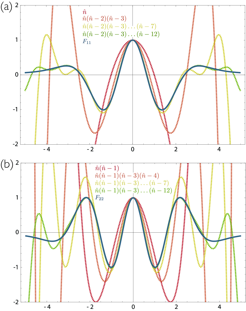
Figure 3: The convergence of the $\hat{n}$ polynomials to their corresponding pattern functions for a photon number measurement of (a) $n=1$ and (b) $n=2$. The polynomials are scaled so that $\mathcal{P}(X)=1$ at $X=0$.

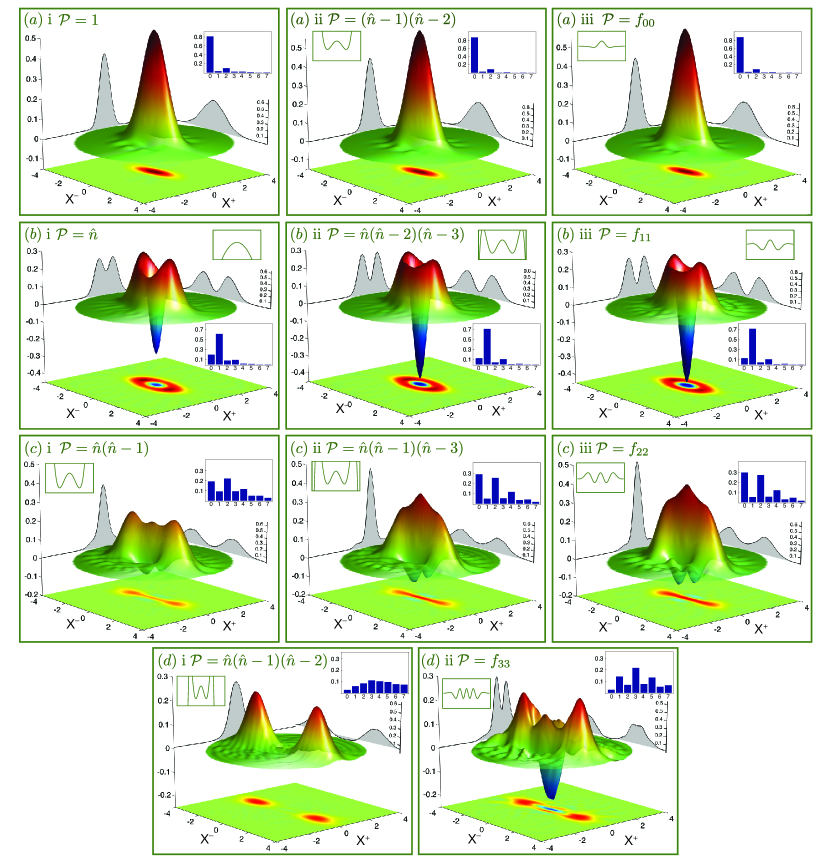
Figure 4: Reconstructed Wigner functions of the: (a) $\mathrm{i}$ measured squeezed vacuum state and (a)$\mathrm{ii}$ and $\mathrm{iii}$ $0$-PSSV state, (b) $1$-PSSV state, (c) $2$-PSSV state, and (d) $3$-PSSV state and their corresponding photon number populations (up to $n=7$), obtained from the reconstructed density matrix. Insets show the conditioning functions for each reconstruction. The Wigner functions are normalised such that the vacuum state has a variance of $\tfrac{1}{4}$.

Our experimental setup is detailed in Fig.2. A shot-noise limited 1064 nm Nd:YAG continuous wave (CW) laser provides the laser source for this experiment. A portion of the 1064 nm light is frequency doubled to provide a pump field at 532 nm. Both fields undergo spatial and frequency filtering to provide shot-noise limited light at the sideband frequencies above 2 MHz. A doubly-resonant optical parametric amplifier in a bow-tie geometry provides a squeezed vacuum resource at the sidebands centred around the carrier. The resulting squeezed coherent state is then displaced to remove much of the intensity of the carrier field. The interference also provides classical amplitude and phase modulation signals, which was introduced on the reference beam, to control of the tomographic angle. The resulting dim squeezed state is then split, with typically 10% reflected towards the conditioning stage and subsequently sampled via phase randomised homodyne detection. The remaining transmitted 90% is measured via tomographic homodyne detection, consisting of sampling $X_{b}^{\theta}$ for 12 values from $\theta=0\ldots 165^{\circ}$. The proportion of light reflected for conditioning is sometimes increased to 15% or 20% to make unlikely events more statistically accessible. This is done at the expense of the state fidelity. Accurate state reconstruction with the techniques presented here relies on experimentally realising a phase-randomised homodyne detection with equal representation of all angles. This is experimentally realised by sweeping the phase of the homodyne over a few $\pi$ at approximately 100 Hz—significantly faster than the drift of the global phase of the lasers. The encoding of phase and amplitude modulation sidebands to allow control of the homodyne angle $X^{\theta}_{b}$ for tomographic reconstruction also allows us to verify that our conditioning measurement $X^{\phi}_{a}$ is appropriately phase-randomised.

These two homodyne detections sample the sideband frequencies between 3–5 MHz, collecting typically $10^{8}$ samples per homodyne angle for both characterisation and conditioning. The probability distributions for the directly measured squeezed state $X^{\theta}_{b}$ is reconstructed for the 12 measured values of $\theta$. We then employ a maximum entropy state estimation (as originally defined in [24]) permitting a Hilbert space up to $n$=30. The maximum entropy state estimation gives the most mixed state consistent with our measured statistical ensemble.

4 Results

If we first ignore the role of conditioning, the ensemble of homodyne measurements at the tomographic characterisation stage allows construction of the histograms describing the probability distribution of each measured $X^{\theta}_{b}$. To achieve this, for each sample, $X^{\theta}_{b}$, we increment the relevant bin by one. One can then reconstruct the Wigner function of the state sampled at the tomographic homodyne detection (Figure 4(b)i) using the maximum entropy state estimation principle [24]. The extension to ‘conditioning’ in post-processing is implemented as follows. For each sample $X^{\theta}_{b}$ we have a corresponding measurement of mode $a$, $X^{\phi}_{a}$, which provides the value for the relevant weighting. Instead of incrementing the bin corresponding to $X^{\theta}_{b}$ by one, we increment the bin by the outcome of a function of our choosing $\mathcal{P}(X_{a}^{\phi})$.

In Figure 4 (b) we focus on the reconstruction of the 1-PSSV state. Figure 4 (a) $\mathrm{i}$ shows the Wigner function obtained using the simplest conditioning polynomial, $\mathcal{P}(X^{\phi}_{a})=\hat{n}_{a}$. This should ideally remove any contributions corresponding to a measurement of $n_{a}=0$ (vacuum) in mode $a$. All other contributions remain and their contributions are additionally weighted by their corresponding eigenvalues, $n_{a}$. In essence we reconstruct a statistical mixture of primarily the $1$-PSSV and $2$-PSSV states, where their contributions are not solely weighted by the likelihood of successful ‘conditioning’, but additionally by their corresponding eigenvalue. For instance, the contributions from $n_{a}=2$ are weighted at twice that of contributions from $n_{a}=1$.

An idealised implementation of a photon annihilation corresponds to a beam splitter with reflectivity approaching zero. This permits statistical isolation of a single photon subtraction event from the considerably less likely two photon subtraction event. However, with an experimental implementation, the requirement of a finite tap-off (typically around 10%) inevitably introduces spurious higher order photon subtraction contributions.

One can instead consider a higher order polynomial in $\hat{n}_{a}$ that removes potential contributions to the reconstructed state from higher order subtractions that are unwanted and are sufficiently statistically significant to warrant removal. As the ideal squeezed vacuum populates only the even photon number pairs, the ideal subtraction of one photon from squeezed vacuum should produce a superposition of the odd photons numbers (and remove any vacuum contribution). Figure 4 (b) $\mathrm{ii}$ demonstrates the dramatic improvement in the reconstructed $1$-PSSV state by implementing the conditioning polynomial $\mathcal{P}(X^{\phi}_{a})=\hat{n}_{a}(\hat{n}_{a}-2)(\hat{n}_{a}-3)$, removing polluting contributions from the $2$ and $3$ photon subtractions. The $F_{11}$ pattern function allows an ideal implementation of a one photon conditioning in mode $a$ (Figure 4 (b)$\mathrm{iii}$). The results of Figure 4 (b) $\mathrm{ii}$ and $\mathrm{iii}$ are markedly similar (sharing a fidelity of 99.2%) despite the clear departure of the polynomials, especially noting how rapidly the polynomial $\hat{n}_{a}(\hat{n}_{a}-2)(\hat{n}_{a}-3)$ diverges in $X^{\phi}_{a}$ (Figure 3).

Figure 4 (c) compiles the results of the $2$-PSSV state reconstruction. Figure 4 (c) $\mathrm{i}$ considers the $\mathcal{P}(X^{\phi}_{a})=\hat{n}_{a}(\hat{n}_{a}-1)$, removing contributions corresponding to a photon number measurement of $n_{a}=0$ and $n_{a}=1$. The ideal reconstructed $2$-PSSV state has high fidelity with the even kitten state. When we additionally correct for the contributions of the $3$-PSSV state there is a clear improvement (Figure 4 (c) $\mathrm{ii}$) in the purity of the reconstructed state, evidenced by the increasing isolation of the even-photon number contributions to the photon number populations. If we consider the relevant pattern function $\mathcal{P}(X^{\phi}_{a})=F_{22}$ (Figure 4 (c) $\mathrm{iii}$) we see a further improvement in the purity of the reconstructed state.

There a handful of subtleties involved in the estimation of the photon statistics with homodyne measurements. Analogies with many of these can be drawn with the usual problems that afflict photon counting measurements. This technique relies on correlations shared between modes $a$ and $b$, and may be degraded by any process that introduces uncorrelated classical or quantum noise. With the results presented here, the significance of electronic noise in detection is understood to be negligible. As we adopt an inherently ‘ensemble’ approach, by making the assumption that the dark noise is uncorrelated to the quantum state we could realise a dark noise correction for both our conditioning in mode $a$ and our characterisation in mode $b$. In reality, the dark noise is sufficiently negligible that any correction proves insignificant. Experimentally, we typically enjoy greater than 18 db dark noise clearance over our measurement band.

However, we are still exposed to the effects of loss. Any loss of purity on the initial squeezed vacuum state constrains the non-Gaussian nature of the reconstructed state. The role of loss can be accurately modelled as a beam-splitter with transmissivity $\lambda$. The role of loss can be understood in by drawing analogy to traditional photon counting. Inefficiencies arising from imperfect homodyne detection efficiency or transmission losses scale the rate of success of the homodyne conditioning, analogous to loss on a photon counting measurement. Whilst here we cannot refer to individual events, as this approach succeeds by considering the entire ensemble, we essentially require a larger ensemble to obtain the same conditioned statistics. Additionally, it can also lead to erroneous conditioning, where a loss of photon may see a 3-photon subtraction event contributing as two photon subtraction.

Our homodyne efficiency is typically 98%, with a fringe visibility of typically $99.2\%$ and specified photodiode quantum efficiency of $\geq 99\%$. Our primary source of loss in the experiment arises from the impurity of the squeezed vacuum resource—and this is most evident with the reconstruction of the 3-PSSV state (Figure 4 (d)). Endeavouring to reconstruct the 3-PSSV state, we optimised the experimental parameters to increase the likelihood of having 3 photons in mode $a$ without sacrificing the quality of the reconstructed state. The likelihood of encountering a 3 photon subtraction event is low. Whilst the probability of subtracting $n$-photons with a beam splitter of reflectivity $\eta$ scales as $\eta^{n}$, attempting to measure 3 or 4 photons from mode $a$ also enforces the additional requirement of having at least $4$ photons in the original squeezed vacuum mode. As a result, the likelihood of having 3 or more photons in mode $a$ scales poorly. We can improve this predicament by firstly increasing the percentage of the input mode used for conditioning (typically 15%) and secondly, by using a stronger squeezed resource, enhancing population of the higher order photon pairs. Increasing the squeezing level is detrimental to the squeezing purity as it introduces noise sources only dominant at high pump power, such as phase noise. In our doubly-resonate system the requirement of the stronger pump field also has consequences for the long-term stability of the experiment. Obtaining sufficient statistics requires longer acquisition time which concatenates the typical experimental drifts in the measured tomographic angle $\theta$, alignment and squeezing levels over time, reducing the overall purity of the reconstructed state. As a result the reconstructed $3$-PSSV state in Figure 4 (d) has lower reconstructed state purity (evidenced by the smaller observable negativities at the origin) than the reconstructed $1$ and $2$-PSSV states which require smaller data sets.

If we attempt to reconstruct the $3$-PSSV state with an additional correction for the $4$ photons events in mode $a$, the reconstructed state becomes noisier. It is not immediately apparent that removing unwanted contributions should introduce statistical noise into the ensemble, but the conditioning on higher photon numbers or the removal of higher order terms essentially requires extraction of finer correlations between modes $a$ and $b$. For a polynomial $\mathcal{P}(n_{a})$ of degree $k$, we essentially estimate moments of $X^{\phi}_{b}$ up to order $2k$. When coupled with the rapid divergence of the polynomials in $X^{\phi}_{b}$, sufficient statistics must be acquired to minimise error. This prevents us from implementing a purification of the $3$-PSSV state in figure 4 (d) with the polynomial approach, even though it is successful with the corresponding $F_{33}$ pattern function (figure 4 (d) $\mathrm{ii}$).

While the pattern functions extract the statistics of ideal photon number discriminating measurement at mode $a$, limited only by the experimental imperfections, it is worth noting that one can essentially obtain the same outcome by implementing a polynomial weighting to only a few orders. This is despite the fact the polynomials calculated to any $\mathcal{P}(\hat{n_{a}})$ will diverge for sufficiently large $X^{\theta}_{b}$. In spite of the clear divergence between polynomial $\hat{n}_{a}(\hat{n}_{a}-1)(\hat{n}_{a}-3)$ and the corresponding pattern function $F_{22}$ (Figure 3 (b)), the corresponding Wigner functions (Figure 4 (c) $\mathrm{ii}$ and $\mathrm{iii}$ share a fidelity of $98.8$%. To emulate a conditioning photon number measurement a low order implementation of the $\hat{n}$ polynomials is generally sufficient.

As a small aside, we also consider the effect of measuring no photons in the conditioning mode (Figure 4 (a) ii and iii). This projects onto a subset of weaker squeezed vacuum input states. This can be compared to the action of de-amplification with a noiseless linear amplifier with a gain $<1$.

5 Conclusion

In this paper we have experimentally demonstrated a technique to reconstruct the Wigner functions of various non-Gaussian states of light with only homodyne measurements. This technique relies on an ensemble based post-processing of the homodyne data informed by a phase randomised homodyne measurement. While it therefore never allows us to prepare a non-Gaussian state, it still enables their characterisation. Using these methods, we were able to reconstruct a 1-PSSV, 2-PSSV and 3-PSSV. Previously, extracting such statistics would have required a full tomographic reconstruction of the two-mode Wigner function. These techniques allow for complete characterisation of the outcome of a conditional measurement on a system, and might prove useful in systems where measurements of the DV of the system are limited or unavailable.

This research was conducted by the Australian Research Council Centre of Excellence for Quantum Computation and Communication Technology (Project number CE110001027).

Appendix A Conditioning Polynomials

In this appendix, we demonstrate how the sampling polynomials can be obtained for arbitrary functions of $\hat{n}$. We provide two equivalent methods for doing this.

The first method involves writing the polynomial functions of the phase randomised quadrature operators $\bar{X}$ in terms of $\hat{n}$ via the creation and annihilation operators. These functions can then be inverted to solve for functions of $\hat{n}$ in term of $\bar{X}$.

The second method reproduce the same polynomials via measuring the moment of the Fock state by integration of Hermite polynomials.

Method 1

For an arbitrary function of $f(\hat{n})$, the analogue of equation (1) that we want to estimate using a phase randomised homodyne measurement would be

$$f\left(X_{b}^{\theta}\right) =\textrm{tr}\left\{\hat{\rho}_{ab}f(\hat{n})\otimes\left|{X_{b}^{\theta}}\right\rangle\left\langle{X_{b}^{\theta}}\right|\right\}$$ (44)

$$=\mathrm{pr}(X_{b}^{\theta})\textrm{tr}_{a}\left\{\hat{\rho}_{a}(X_{b}^{\theta})f(\hat{n})\right\}\;,$$ (45)

where $\rho_{a}(X_{b}^{\theta})$ is the state at $a$ after tracing out $b$. Our goal is to find a function $F(\bar{X})$ corresponding to $f(\hat{n})$ such that

$$\textrm{tr}\left\{\hat{\rho}f(\hat{n})\right\}=\textrm{tr}\left\{\hat{\rho}F(\bar{X})\right\}\;,$$ (46)

where

$$F(\bar{X})=\frac{1}{2\pi}\int_{0}^{2\pi}\,d\theta F(\hat{a}_{\phi}+\hat{a}_{\phi}^{\dagger})$$ (47)

and $\hat{a}_{\phi}=\hat{a}\exp(-i\phi)$. Let us consider polynomial functions of $\bar{X}$ for which the monomials $\bar{X}^{m}$ for $m=0,1,\ldots$ forms a basis.

For all odd values of $m$, $\bar{X}^{m}$ vanish since the exponential terms $\exp(-i\phi)$ integrate to zero. For even $m$, the only terms in the expansion of $(\hat{a}_{\phi}+\hat{a}_{\phi}^{\dagger})^{m}$ that are not a function of $\phi$ are those having equal numbers of $\hat{a}_{\phi}$ and $\hat{a}_{\phi}^{\dagger}$. These are the only terms that are non-zero after performing the integral in equation (47). They can be expressed as a function of $\hat{n}$ using the identity $\hat{a}^{\dagger}\hat{a}=\hat{n}$ and the commutation relation $[\hat{a},\hat{a}^{\dagger}]=1$.

We provide an example for the case of $m=4$:

$$\bar{X}^{4} =\frac{1}{2\pi}\int_{0}^{2\pi}d\phi\left(\hat{a}_{\phi}+\hat{a}_{\phi}^{\dagger}\right)^{4}$$ (48)

$$=\hat{a}\hat{a}\hat{a}^{\dagger}\hat{a}^{\dagger}+\hat{a}\hat{a}^{\dagger}\hat{a}\hat{a}^{\dagger}+\hat{a}\hat{a}^{\dagger}\hat{a}^{\dagger}\hat{a}$$ (49)

$$+\hat{a}^{\dagger}\hat{a}^{\dagger}\hat{a}\hat{a}+\hat{a}^{\dagger}\hat{a}\hat{a}^{\dagger}\hat{a}+\hat{a}^{\dagger}\hat{a}\hat{a}\hat{a}^{\dagger}$$ (50)

$$=6\hat{n}^{2}+6\hat{n}+3\;.$$ (51)

Results for various powers of $\bar{X}$ are tabulated below.

$$\bar{X}^{0} =1$$

$$\bar{X}^{2} =1+2\hat{n}$$

$$\bar{X}^{4} =3+6\hat{n}+6\hat{n}^{2}$$

$$\bar{X}^{6} =15+40\hat{n}+30\hat{n}^{2}+20\hat{n}^{3}$$

$$\bar{X}^{8} =105+280\hat{n}+350\hat{n}^{2}+140\hat{n}^{3}+70\hat{n}^{4}$$

$$\bar{X}^{10} =945+2898\hat{n}+3150\hat{n}^{2}+2520\hat{n}^{3}+630\hat{n}^{4}+252\hat{n}^{5}$$

Method 2

As an alternative method, we note that equation (46) must hold for arbitrary inputs $\hat{\rho}$. In particular, when $\hat{\rho}=\left|{n}\right\rangle\left\langle{n}\right|$ we get

$$\textrm{tr}\left\{F(\bar{X})\left|{n}\right\rangle\left\langle{n}\right|\right\} =f(n)$$ (52)

$$\iint dxd\tilde{x}\,\phi_{n}(x)\phi^{\star}_{n}(\tilde{x})F(x)\delta(x-\tilde{x}) =f(n)$$ (53)

$$\int dx\,\left|\phi_{n}(x)\right|^{2}F(x) =f(n)$$ (54)

where $\phi_{n}(x)=\left<n|x\right>$ are the eigenstates of the harmonic oscillators. For $F(\bar{X})=\bar{X}^{m}$, the associated functions of $n$ would correspond to the $m$-th moment of the eigenstates.

While this integration can be performed directly using the Hermite polynomials, it turns out that it is more convenient to express $\bar{X}$ in terms of the annihilation and creation operators instead. As an example, we evaluate $f(n)$ when $F(\bar{X})=\bar{X}^{4}$:

$$\left\langle{n}\right|\bar{X}^{4}\left|{n}\right\rangle =\frac{1}{2\pi}\int_{0}^{2\pi}d\phi\left\langle{n}\right|\left(\hat{a}_{\phi}+\hat{a}_{\phi}^{\dagger}\right)^{4}\left|{n}\right\rangle$$ (55)

$$=\left\langle{n}\right|\hat{a}\hat{a}\hat{a}^{\dagger}\hat{a}^{\dagger}+\hat{a}\hat{a}^{\dagger}\hat{a}\hat{a}^{\dagger}+\hat{a}\hat{a}^{\dagger}\hat{a}^{\dagger}\hat{a}$$ (56)

$$+\hat{a}^{\dagger}\hat{a}^{\dagger}\hat{a}\hat{a}+\hat{a}^{\dagger}\hat{a}\hat{a}^{\dagger}\hat{a}+\hat{a}^{\dagger}\hat{a}\hat{a}\hat{a}^{\dagger}\left|{n}\right\rangle$$ (57)

$$=6n^{2}+6n+3\;$$ (58)

which is the same result as equation (51) as to be expected.

References

References

- [1] U. Leonhardt, H. Paul, and G. M. D’Ariano. Tomographic reconstruction of the density matrix via pattern functions. Physical Review A, 52:4899–4907, Dec 1995.
- [2] Th. Richter. Determination of photon statistics and density matrix from double homodyne detection measurements. Journal of Modern Optics, 45(8):1735–1749, August 1998.
- [3] T. Ralph, W. Munro, and R. Polkinghorne. Proposal for the Measurement of Bell-Type Correlations from Continuous Variables. Physical Review Letters, 85(10):2035–2039, September 2000.
- [4] T. C. Ralph, E. H. Huntington, and T. Symul. Single-photon side bands. Physical Review A, 77(6):1–7, June 2008.
- [5] K. Banaszek. Maximum likelihood estimation of photon number distribution from homodyne statistics. arXiv.org, 1997.
- [6] M. Vasilyev, S. K. Choi, P. Kumar, and G. M. D’Ariano. Tomographic measurement of joint photon statistics of the twin-beam quantum state. Physical Review Letters, 84(11):2354–2357, 2000.
- [7] J. G. Webb, T. C. Ralph, and E. H. Huntington. Homodyne measurement of the average photon number. Physical Review A, 73(3):1–7, March 2006.
- [8] N. B. Grosse, T. Symul, M. Stobińska, T. C Ralph, and P. K. Lam. Measuring Photon Antibunching from Continuous Variable Sideband Squeezing. Physical Review Letters, 98(15):1–4, April 2007.
- [9] J. Eisert, S. Scheel, and M. B. Plenio. Distilling Gaussian states with Gaussian operations is impossible. Physical Review Letters, 89(13):137903, 2002.
- [10] G. Giedke and J. I. Cirac. Characterization of Gaussian operations and distillation of Gaussian states. Physical Review A, 66(3):32316, 2002.
- [11] P. Van Loock. Optical hybrid approaches to quantum information. Laser & Photonics Reviews, 5(2):167–200, 2011.
- [12] H.M. Chrzanowski, J. Bernu, B. Sparkes, B. Hage, A. P. Lund, T.C. Ralph, P. Lam, and T. Symul. Photon-number discrimination without a photon counter and its application to reconstructing non-Gaussian states. Physical Review A, 84(5), November 2011.
- [13] M. Dakna, T. Anhut, T. Opatrný, .L Knöll, and D. G. Welsch. Generating Schrödinger-cat-like states by means of conditional measurements on a beam splitter. Physical Review A, 55(4):3184–3194, 1997.
- [14] A. Gilchrist, K. Nemoto, W. J. Munro, T. C. Ralph, S. Glancy, S. L. Braunstein, and G. J. Milburn. Schrödinger cats and their power for quantum information processing. Journal of Optics B: Quantum and Semiclassical Optics, 6:S828, 2004.
- [15] A. P. Lund, T. Ralph, and H. Haselgrove. Fault-Tolerant Linear Optical Quantum Computing with Small-Amplitude Coherent States. Physical Review Letters, 100(3):030503, January 2008.
- [16] T. Opatrný, G. Kurizki, and D. G. Welsch. Improvement on teleportation of continuous variables by photon subtraction via conditional measurement. Physical Review A, 61(3):32302, 2000.
- [17] A. Ourjoumtsev, A. Dantan, R. Tualle-Brouri, and P. Grangier. Increasing Entanglement between Gaussian States by Coherent Photon Subtraction. Physical Review Letters, 98(3):1–4, 2007.
- [18] A. Ourjoumtsev, H. Jeong, R. Tualle-Brouri, and P. Grangier. Generation of optical ‘Schrödinger cats’ from photon number states. Nature, 448:784–786, 2007.
- [19] A. Ourjoumtsev, R. Tualle-Brouri, J. Laurat, and P. Grangier. Generating Optical Schrödinger Kittens for Quantum Information Processing. Science, 312(5770):83–86, 2006.
- [20] J. S. Neergaard-Nielsen, B. M. Nielsen, C. Hettich, K. Mølmer, and E. S. Polzik. Generation of a superposition of odd photon number states for quantum information networks. Physical Review Letters, 97(8):83604, 2006.
- [21] K. Wakui, H. Takahashi, A. Furusawa, and M. Sasaki. Photon subtracted squeezed states generated with periodically poled KTiOPO4. Opt. Express, 15(6):3568–3574, March 2007.
- [22] T. Gerrits, S. Glancy, T. Clement, and B. Calkins. Generation of optical coherent-state superpositions by number-resolved photon subtraction from the squeezed vacuum. Physical Review A, 2010.
- [23] U. Leonhardt, M. Munroe, T. Kiss, T. Richter, and M. G. Raymer. Sampling of photon statistics and density matrix using homodyne detection. Optics communications, 127(1-3):144–160, 1996.
- [24] V. Buzek and G. Drobny. Quantum tomography via the MaxEnt principle. Journal of Modern Optics, 47(14):2823–2839, November 2000.