Entanglement in non-critical inhomogeneous quantum chains

Abstract

We study an inhomogeneous critical Ising chain in a transverse field whose couplings decay exponentially from the center. In the strong inhomogeneity limit we apply Fisher’s renormalization group to show that the ground state is formed by concentric singlets similar to those of the rainbow state of the XX model. In the weak inhomogeneity limit we map the model to a massless Majorana fermion living in a hyperbolic spacetime, where, using CFT techniques, we derive the entanglement entropy that is violated linearly. We also study an inhomogeneous non-critical Ising model that for weak inhomogeneity is mapped to a massive Majorana fermion, while for strong inhomogeneity regime it exhibits trivial and non-trivial topological phases and a separation between regions with high and low entanglement. We also present the entanglement Hamiltonian of the model.

I Introduction

The study of entanglement in quantum many-body systems Amico.08 ; Calabrese.09b ; Laflorencie.16 ; Roy.19 has proven to be an excellent way to advance in the understanding of quantum matter Wen.book . Given a pure state $\ket{\Psi}$ of a system and a bipartition into two subsystems, $A\cup B$, all the information concerning quantum correlations between these parts is contained in the reduced density matrix $\rho_{A}=\Tr_{B}\ket{\Psi}\bra{\Psi}$. The most important measure of entanglement is the von Neumann entropy, $S_{A}=-\Tr\rho_{A}\log\rho_{A}$, that vanishes if and only if the subsystems are disentangled. The low energy states of local quantum Hamiltonians are expected to satisfy the so-called area law, which asserts that the entanglement entropy (EE) of a block is bounded by the size of its boundary Sredniki.93 ; Wolf.08 ; Hastings.06 ; Eisert.10 . This property holds for one dimensional gapped Hamiltonians under certain assumptions Hastings.06 , but is violated in critical Hamiltonians described by a conformal field theory (CFT), where the EE grows logarithmically with the subsystem size and is proportional to the central charge Holzhey.94 ; Vidal.03 ; Calabrese.04 ; Calabrese.09 .

The study of entanglement in spatially inhomogeneous systems has attracted recently considerable interest. For example, the EE of local Hamiltonians with random couplings exhibits a logarithmic behaviour, presenting some similarity with the CFT result Refael.04 ; Refael.04b ; Laflorencie.05 ; Fagotti.11 ; Ramirez.14 ; Ruggiero.16 . Other interesting cases include the engineered trapping potentials for ultracold atoms which reduce the boundary effects Nishino.09 ; Campostrini.10 ; Dubail.17 ; Murciano.19 , the interplay between quantum gravity and strange metals within the SYK model Sachdev.93 ; Rosenhaus.19 , or the quantum simulation of the Dirac vacuum on a curved spacetime using optical lattices Boada.11 ; Laguna.17 ; Mula.21 . In some cases, it is possible to obtain the GS of these systems using renormalization group (RG) schemes such as the Dasgupta-Ma procedure Dasgupta.80 . Conversely, the RG can help us design certain lattice models, such as the rainbow state (RS), which is the GS of an XX spin-chain whose couplings decay exponentially from the center towards the edges, and which presents a linearly growing EE between its two halves Vitagliano.10 ; Ramirez.14b ; Alkurtass.14 ; Ramirez.15 ; Samos.19 ; Laguna.16 ; Laguna.17b ; Tonni.18 ; MacCormack.18 ; Samos.20 ; AA18 ; Alba.19 . The system is described in terms of an inhomogeneity parameter $h$, associated to the exponential decay. In the strong inhomogeneity regime, the GS is a nested set of Bell pairs, which can also be described as a concentric singlet state Vitagliano.10 ; Alkurtass.14 . In the weak inhomogeneity regime the rainbow chain corresponds to a free Dirac theory on a (1+1)D anti-de-Sitter space-time Laguna.17b ; MacCormack.18 . Thus, the EE can be obtained as a deformation of well known results from CFT, showing that the logarithmic growth maps into a linear one. Moreover, there is a smooth crossover between the weak and strong inhomogeneity regimes.

In addition to the EE, bipartite entanglement can be characterized by other magnitudes. The density matrix $\rho_{A}$ can be written as

$$\rho_{A}\propto e^{-\mathcal{H}_{A}},$$ (1)

where $\mathcal{H}_{A}$ is called the entanglement Hamiltonian (EH) associated to a block $A$ within a quantum state Li_Haldane.08 ; BW.75 ; BW.76 ; Peschel.09 ; Cardy.16 ; Eisler.19 ; Eisler.20 . Even if the original state is translationally invariant, the EH usually represents an inhomogeneous system, and it has been characterized for several interesting systems, employing e.g. the corner matrix formalism (CTM) Peschel.09 ; Eisler.20 or CFT results Cardy.16 . Moreover, the EH of certain inhomogeneous systems has been described using the RS as a benchmark, showing that it can be understood as a thermofield double: each half of the system can be approximated by a homogeneous system at a finite temperature that depends on the inhomogeneity level $h$ Tonni.18 . The spectrum of the EH is called the entanglement spectrum (ES), which can provide interesting information e.g. regarding the existence of symmetry-protected topological phases (SPT) Kitaev.01 ; Pollman10 ; Fidkowski2011 ; Turner2011 ; W11a ; P12 .

The aim of the present work is twofold. First, to characterize the emergence of a rainbow state as a ground state of an inhomogeneous transverse field Ising (ITF) Hamiltonian, when the couplings and the external fields are allowed to decay in a certain way, by mapping it to a (1+1)D massless Majorana field on a curved space-time. Then, we will describe the structure of the model away from the critical point, showing that it reduces to a massive Majorana field in the same setup. Moreover, we shall also consider the relation between our model and the Kitaev chain Kitaev.01 .

This article is organized as follows. In section II we introduce an inhomogeneous version of the ITF model and describe its entanglement structure. The strong inhomogeneity regime is discussed by means of RG schemes, and the weak inhomogeneity regime is characterized via field theory methods. In Sec. III we propose a variation of the previous model by adding a new parameter which shifts it away from the critical point, and we describe its entanglement properties in the strong and weak inhomogeneity regimes. Finally, we present a brief discussion of our conclusions and prospects in Sec. IV.

II The Ising Rainbow State

Let us consider an inhomogeneous ITF open spin $1/2$ chain with an even number of sites $N=2L$ whose Hamiltonian is defined as:

$$H_{I}=-\sum_{m=-L+1/2}^{L-3/2}J_{m}\sigma^{z}_{m}\sigma^{z}_{m+1}-\sum_{m=-L+1/2}^{L-1/2}\Gamma_{m}\sigma^{x}_{m},$$ (2)

where $\sigma^{x}$ and $\sigma^{z}$ are Pauli matrices. Notice that the spins are indexed by half-odd integers for later convenience, $m=-L+1/2,\dots,L-1/2$. We shall apply a Jordan-Wigner transformation and write Eq. (2) in terms of Dirac fermions $c^{\dagger}_{m}$ which satisfy the usual anti-commutation relations $\{c^{\dagger}_{m},c_{n}\}=\delta_{mn}$, and then decompose them in terms of Majorana fermions

$$c_{m}=\frac{1}{2}(\alpha_{m}+i\beta_{m}),$$ (3)

that satisfy the anti-commutation relations $\{\alpha_{m},\alpha_{n}\}=\{\beta_{m},\beta_{n}\}=2\delta_{mn}$ and $\{\alpha_{m},\beta_{n}\}=0$. In terms of these Majorana fermions Eq. (2) reads:

$$H= -i\Bigl{(}\sum_{m=1/2}^{L-1/2}\Gamma_{m}\left(\alpha_{m}\beta_{m}+\alpha_{-m}\beta_{-m}\right)$$ (4)

$$+\sum_{m=1/2}^{L-3/2}J_{m}\left(\beta_{m}\alpha_{m+1}+\beta_{-(m+1)}\alpha_{-m}\right)+J_{-1/2}\beta_{-1/2}\alpha_{1/2}\Bigr{)},$$

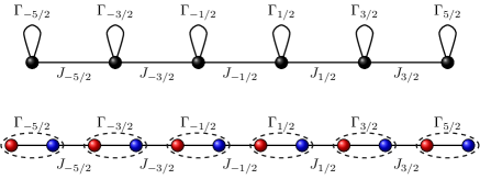
Figure 1: Spin (top) and Majorana fermion (bottom) representations of the inhomogeneous ITF model. The red (blue) points correspond to $\alpha$ ($\beta$) Majorana fermions.

Notice that the same system is described by $2L$ spins and $4N$ Majorana fermions. In Fig. 1 we present an schematic representation of the model in terms of spins (top) and Majorana fermions (bottom). The transverse field $\Gamma_{m}$ couples two Majorana fermions with the same index $(\alpha_{m},\beta_{m})$, while the coupling constants $J_{m}$ link Majorana fermions with different indices $(\beta_{m},\alpha_{m+1})$. The dashed lines that encircle the Majorana fermions represent the Dirac fermions $c_{m}$ in Eq. (3).

Notice that if $J_{m}=\Gamma_{m}=1$ for all $m$ we recover the critical ITF model whose low-energy behaviour is described by the two dimensional Ising CFT with central charge $c=1/2$. In addition, if $J_{m}=0$ for all $m$, the ground state becomes a trivial product state built upon the physical fermions $c_{m}$. On the contrary, if $\Gamma_{m}=0$ for all $m$, the Majorana fermions placed at the edges of the Majorana chain, $\alpha_{-L+1/2}$ and $\beta_{L-1/2}$, do not appear in the Hamiltonian, Eq. (4). Moreover, they correspond to Majorana zero modes and the GS belongs to the topologically non-trivial phase of the Kitaev model Kitaev.01 .

Let us consider both the spin and the Majorana fermion Hamiltonians, Eqs. (2) and (4), under the following choice of coupling constants $J_{m}$ and $\Gamma_{m}$:

$$J_{m} = \begin{cases}e^{-2h|m+1/2|}&\text{if }m\neq-1/2,\\ e^{-h/2}&m=-1/2,\\ \end{cases}$$

$$\Gamma_{m} = e^{-2h|m|},$$ (5)

where $h\geq 0$ is the inhomogeneity parameter. Notice that for $h>0$ the intensity of the couplings decreases from the center towards the edges, with $J_{-1/2}$ corresponding to the strongest coupling. Also, the system is symmetric under reflections around the central bond, satisfying $J_{-(m+1)}=J_{m}$ and $\Gamma_{m}=\Gamma_{-m}$. In the remainder of this section, we shall describe the strong ($h\gg 1$) and weak ($h\ll 1$) inhomogeneity regimes.

II.1 Strong Inhomogeneity

In the limit $h\gg 1$ we can characterize the GS of (4) using the strong disorder renormalization scheme (SDRG) developed by Fisher for the ITF Fisher.94 ; Fisher.95 . It proceeds by finding the strongest interaction coupling, either $\Gamma$ or $J$, which gets sequentially decimated. If it corresponds to a magnetic field, $\Gamma_{i}$, the $i$-th spin is integrated out, leaving the system with one spin less and a new coupling term between the spins $i-1$ and $i+1$,

$$\tilde{J}_{i-1}\sigma^{z}_{i-1}\sigma^{z}_{i+1},\qquad\text{ with }\;\;\tilde{J}_{i-1}=\frac{J_{i-1}J_{i}}{\Gamma_{i}}.$$ (6)

On the other hand, if the coupling $J_{i}$ is the strongest interaction at a given RG step, the spins $i$ and $i+1$ get renormalized into a single spin with effective Hamiltonian

$$\tilde{\Gamma}_{i}\sigma^{x}_{i},\qquad\text{ with }\tilde{\Gamma}_{i}=\frac{\Gamma_{i}\Gamma_{i+1}}{J_{i}}.$$ (7)

Notice that renormalizing a $J$ term entangles two neighboring spins, while the renormalization of a $\Gamma$ term freezes that spin along the direction of the magnetic field, and decouples it from the chain.

It can be shown that the fusion rules of Majorana fermions correspond to the $SU(2)_{2}$ quantum group Bonesteel.07 ; Pachos.17 ; Pachos.book ; Sierra.book ; Nayak.08 . The non-univocal fusion rule

$$\frac{1}{2}\crossproduct\frac{1}{2}=0+1,$$ (8)

corresponds to the pairing of two Majorana fermions, for instance $\alpha_{m}\beta_{m}$, which in terms of of Dirac fermions is $2\left(c^{\dagger}_{m}c_{m}-1/2\right)$, see Eq. (3), and we can attach the fusion channel $0$ ($1$) to the $-1$ ($+1$) eigenvalue. Indeed, notice that Eq. (8) reminds the composition of two $1/2$ spins. Thus, we may call the less energetic channel a generalized singlet state Bonesteel.07 ; Fidkowsky.08 , and the other channel as a generalized triplet (albeit there is no $S_{z}$ degeneracy). Notice that while the $1/2$ spins obey the $SU(2)$ algebra and the singlet states span the total $S_{z}=0$ Hilbert space sector, Majorana fermions obey the $SU(2)_{k=2}$ algebra and the generalized singlet state spans the Hilbert space sector for the fusion channel $0$.

With this parallelism in mind, we can devise an SDRG specially suited for an inhomogeneous Majorana chain Motrunich.01 ; Devakul.17 , as it is done in Appendix A. At each RG step, the two Majorana fermions linked through the strongest coupling (notice that in terms of Majorana fermions the $J$ and $\Gamma$ terms are equivalent) are fused into their less energetic channel, forming a generalized singlet state or bond, and leaving a renormalized coupling between their closest neighbors. This scheme is completely equivalent to Fisher’s RG, Eqs. (6) and (7). In this case, the SDRG becomes analogous to the Dasgupta-Ma technique for spin-1/2 XX chains Dasgupta.80 , for which it can be proved that the bonds never cross Laguna.16 .

Let us apply this RG scheme to the Majorana Hamiltonian given in Eq. (4). The first Majorana pair to be decimated is $(\beta_{-1/2},\alpha_{1/2})$, because $J_{-1/2}$ is the strongest coupling. Hence, these two Majorana fermions fuse into a Dirac fermion,

$$b_{1/2}=\frac{1}{2}\left(\beta_{-1/2}+i\alpha_{1/2}\right),$$ (9)

which becomes decoupled. Using Eq. (7) we can find an effective Hamiltonian with $2(N-1)$ Majorana fermions, whose new central term $\tilde{\Gamma}_{1/2}\alpha_{-1/2}\beta_{1/2}$ is given by

$$\tilde{\Gamma}_{1/2}=\frac{\Gamma_{-1/2}\Gamma_{1/2}}{J_{-1/2}}=e^{-\frac{3h}{2}}.$$ (10)

The strongest coupling is now $\tilde{\Gamma}_{1/2}$. We apply the RG again, and the decimated Majorana fermions fuse into a Dirac fermion,

$$d_{1/2}=\frac{1}{2}\left(\alpha_{-1/2}+i\beta_{1/2}\right).$$ (11)

The new effective Hamiltonian of $2(N-2)$ Majorana fermions has a central term $\tilde{J}_{3/2}$ which is given by Eq. (6),

$$\tilde{J}_{3/2}=\frac{J_{-3/2}J_{1/2}}{\tilde{\Gamma}_{1/2}}=e^{-\frac{5h}{2}},$$ (12)

which is again the strongest coupling in the chain. Given the symmetry of the coupling constants, Eq. (5), all RG steps decimate the central pair of Majorana fermions, fusing them alternatively into $b$ and $d$ Dirac fermions. Hence, the ground state, that we shall call the Majorana rainbow state $\ket{\text{MRS}}$, is annihilated by the following Dirac operators:

$$b_{m}\ket{\text{MRS}}=0,\quad d_{m}\ket{\text{MRS}}=0,\quad m=\frac{1}{2},\dots,L-\frac{1}{2},\\$$ (13)

with

$$b_{m}=\frac{1}{2}\left(\beta_{-m}+i\alpha_{m}\right),\quad d_{m}=\frac{1}{2}\left(\alpha_{-m}+i\beta_{m}\right).$$ (14)

$\ket{\text{MRS}}$ is a concentric generalized singlet state, shown in Fig. 2.

It is worth to compare the Majorana rainbow state Eq. (13) with its Dirac counterpart, which emerges as the GS of the inhomogeneous XX chain and its fermionic version Ramirez.14b ; Ramirez.15 ; Laguna.16 ; Laguna.17b . This state can be seen as a singlet state of concentric bonding and antibonding operators,

$$\ket{\text{RS}_{\text{XX}}}=\prod_{m=1/2}^{L-1/2}(b^{-}_{m})^{\dagger}(b^{+}_{m})^{\dagger}\ket{0},$$ (15)

with

$$\begin{cases}b^{+}_{m}=\frac{1}{\sqrt{2}}\left(c_{m}+c_{-m}\right)\\ b^{-}_{m}=\frac{1}{\sqrt{2}}\left(c_{m}-c_{-m}\right).\end{cases}$$ (16)

The alternation between bonding and antibonding is due to the non-local nature of the Jordan-Wigner transformation, since each long-distance coupling acquires a phase related to the number of fermions contained in it. In spin language, the XX model $\ket{RS_{\text{XX}}}$ is formed by spin-$1/2$ concentric singlets. The alternation between bonding and antibonding in Eq. (15) is therefore similar to that of $b$ and $d$ Dirac fermions in Eq. (14).

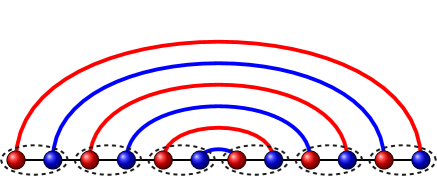
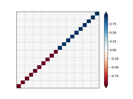
Figure 2: Top: schematic representation of the outcome of the RG for a chain of 6 spins. Blue bonds stand for $b$-type Dirac fermions, while red ones represent $d$-type fermions, see Eq. (14), which can also be considered as generalized singlet states corresponding to the less energetic fusion channel. Bottom: covariance matrix of the RS for $N=20$ and $h=10$. Notice that the non-zero elements are in the anti-diagonal, as it is dictated by the structure of the $b$ and $d$ fermions.

Let us compute the EE of a subsystem $A$, with length $L_{A}$, for the Majorana RS, Eq. (13). The EE of any partition of a ground state formed by $SU(2)$ singlet states can be estimated by counting the number of bonds which cross the partition boundary, and multiplying by $\log(2)$. The procedure is the same when we deal with generalized singlet states. The EE of any subsystem $A$ can be estimated by counting the number of bonds which cross the partition boundary and multiplying by $\log d$ Bonesteel.07 , where $d=\sqrt{2}$ is the associated quantum dimension to the algebra $SU(2)_{2}$.

Alternatively, the EE of a Gaussian state can be obtained from its covariance matrix (CM), $\mathcal{C}$,

$$\mathcal{C}_{ab}=\expectationvalue{[\gamma_{a},\gamma_{b}]},$$ (17)

where we have arranged the Majorana operators in a vector form $\bm{\gamma}^{T}=(\alpha_{-L+1/2},\beta_{-L+1/2},\dots,\alpha_{L-1/2})$. In Appendix B we provide a brief derivation of this expression. The structure of the GS obtained through the decimation procedure shows up in the CM, as we can see in Fig. 2 (b). The EE of a subsystem $A$ with size $L_{A}$ can be computed through the eigenvalues $\pm\lambda_{k}$, $k\in\{1,\cdots,L_{A}/2\}$ of the appropriate restriction $\mathcal{C}_{A}$ of the CM Peschel.03 , through

$$S_{A}=-\sum_{k=1}^{L_{A}}\nu_{k}\log\nu_{k},\qquad\nu_{k}=\frac{1}{2}\left(1+\lambda_{k}\right).$$ (18)

We can now compute the EE of a lateral block of the system, $A_{\ell}=\{-L+1/2\dots-L+1/2+2\ell\}$, with $\ell=1,\cdots,L$. Notice that a block with an odd number of Majorana operators has no physical sense. Thus, $A_{\ell}$ must contain an even number of Majorana fermions, which correspond to the physical fermions (dotted boxes) or the spins (black balls) of Fig. 1. We can obtain the EE by counting the number of bonds $n_{b}$ (reds and blues) that $A_{\ell}$ cuts in Fig. 2 and multiply it by $\log d$.

$$S_{A}=n_{b}\log\sqrt{2}.$$ (19)

Hence, we have that the EE of the MRS grows linearly,

$$S(A_{\ell})=2\ell\log{\sqrt{2}}=\ell\log 2,$$ (20)

and the maximal EE corresponds to the half chain block $S(A_{L})=L\log 2$.

II.2 Weak Inhomogeneity Regime

In this section we shall consider the GS of Eq. (2) with couplings given by Eq. (5), in the low inhomogeneity regime, $h\ll 1$. The equations of motion associated to the lattice Hamiltonian in the Heisenberg picture are given by $i\partial_{t}\alpha_{\pm m}=[H,\alpha_{\pm m}]$ and $i\partial_{t}\beta_{\pm m}=[H,\beta_{\pm m}]$. Using Eq. (4) we have

$$\partial_{t}\alpha_{n} = -2e^{-2h|n|}\left(\beta_{n}-e^{\operatorname{sign}(n)h}\beta_{n-1}\right)$$

$$\partial_{t}\beta_{n} = 2e^{-2h|n|}\left(\alpha_{n}-e^{\operatorname{sign}(n)h}\alpha_{n+1}\right).$$ (21)

Now, we define the fields

$$\alpha_{m}=\sqrt{a}\alpha(x),\quad\beta_{m}=\sqrt{a}\beta(x),$$ (22)

where $a$ is the lattice spacing between the Dirac fermions $c_{m}$, $x=ma$, which satisfy the usual anticommutation relations, $\{\alpha(x),\alpha(x^{\prime})\}=\{\beta(x),\beta(x^{\prime})\}=2\delta(x-x^{\prime})$ and $\{\alpha(x),\beta(x)\}=0$. We find the continuum limit of the lattice equations of motion by plugging these fields into Eqs.(21) and requiring $a\to 0$ and $L\to\infty$ with both $\mathcal{L}=aL$ and $\hat{h}=h/a$ kept constant,

$$\partial_{t}\alpha(t,x) \approx -2ae^{-2\hat{h}|x|}\left(\partial_{x}-\operatorname{sign}(x)\hat{h}\right)\beta(t,x)$$

$$\partial_{t}\beta(t,x) \approx -2ae^{-2\hat{h}|x|}\left(\partial_{x}-\operatorname{sign}(x)\hat{h}\right)\alpha(t,x),$$ (23)

where we made the approximation $e^{\operatorname{sign}(x)h}\approx(1+\operatorname{sign}(x)h)$. If $h=0$ the equations of motion (23) correspond to the massless Dirac equation $i\not{\partial}\Psi=(i\gamma^{0}\partial_{0}+i\gamma^{1}\partial_{1})\Psi=0$, where we have introduced the spinor

$$\Psi^{T}=(\alpha(x^{0},x^{1}),\beta(x^{0},x^{1})),\quad(x^{0},x^{1})=(2t,x).$$ (24)

Our choice for the $\gamma$ matrices is $\gamma^{0}=-\sigma_{2}$, $\gamma^{1}=i\sigma_{3}$ and $\gamma^{3}=\sigma_{1}$, where $\sigma_{i}$, $i=1$, 2, 3, are the Pauli matrices. Hereafter, we choose $a=1$ that sets the Fermi velocity $v_{F}=1$, so we can simplify $\hat{h}=h$, $\mathcal{L}=L$, and rewrite the equations of motion of the inhomogeneous system, Eq. (23), as

$$\left(-\sigma_{2}\partial_{0}+e^{-2h|x^{1}|}i\sigma_{3}\left(\partial_{1}-\text{sign}(x^{1})h\right)\right)\Psi=0\ .$$ (25)

The previous equation corresponds to the massless Dirac equation in a curved spacetime whose metric depends on the inhomogeneity $h$, see Appendix C for details. The Dirac equation on a generic metric can be written as Eq. (88),

$$\left(-\sigma_{2}\partial_{0}+\frac{i}{2}\omega_{0}^{01}\sigma_{3}+\frac{E_{1}^{1}}{E_{0}^{0}}\left(i\sigma_{3}\partial_{1}-\frac{i}{2}\omega_{1}^{01}\sigma_{2}\right)\right)\Psi=0,$$ (26)

where $\omega_{\mu}^{ab}$ is the spin connection and $E_{a}^{\mu}$ is the inverse of the zweibein. Comparing Eq. (26) with our equations of motion Eq. (25), we obtain

$$\frac{E^{1}_{1}}{E^{0}_{0}} = e^{-2h|x^{1}|},$$ (27)

$$\omega^{01}_{0} = -2e^{-2h|x^{1}|}h\text{sign}(x^{1}),$$ (28)

$$\omega^{01}_{1} = 0.$$ (29)

The solution of these equations gives rise to the space-time metric:

$$g_{00}=-e^{-4h|x|},\quad g_{11}=1\ ,$$ (30)

whose Euclidean version is

$$ds^{2}=e^{-4h|x|}dt^{2}+dx^{2}=\Omega^{2}(x)dzdz,$$ (31)

where $\Omega(x)=e^{-2h|x|}$ is the Weyl factor and

$$z=\tilde{x}+it,\quad\text{with}\quad\tilde{x}=\int_{0}^{x}\frac{dy}{\Omega(y)}=\frac{\operatorname{sign}(x)}{2h}\left(e^{2h|x|}-1\right).$$ (32)

The non-zero Christoffel symbols are

$$\Gamma^{0}_{01}=-2h\operatorname{sign}(x),\quad\Gamma^{1}_{00}=-2h\operatorname{sign}(x)e^{-4h|x|},$$ (33)

and the non-zero components of the Ricci tensor are

$$R_{00}=-e^{-4h|x|}\left(4h\delta(x)-4h^{2}\right),\quad R_{11}=4h\delta(x)-4h^{2}.$$ (34)

The scalar of curvature $R=g^{\mu\nu}R_{\mu\nu}$ is

$$R=8\left(h\delta(x)-h^{2}\right),$$ (35)

where we have used Eq. (30). Thus, $R$ is singular at the origin and constant and negative everywhere else, thus allowing for the holographic interpretation of the rainbow state that has been discussed in the literature MacCormack.18 .

II.2.1 Entanglement entropies

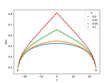
Figure 3: EE of lateral blocks of the GS of Eq. (2) with couplings (5) for different values of $h$ and $L=40$. The dots represent the numerical values obtained by exact diagonalization and the lines correspond to the predictions of Eq. (36) using Eq. (91).

We have shown that the continuum limit of the lattice model Eq. (4) corresponds to a Majorana field in curved space-time, described by a conformal field theory with central charge $c=1/2$. We can obtain the EE of a block within this state employng standard procedures Calabrese.04 , via the correlation function of twist operators in an $n$-times replicated worldsheet Laguna.17b . The EE of the lateral blocks considered in the previous section is

$$S(x)=\frac{1}{12}\log\left(\Omega(x)\frac{8\tilde{L}}{\pi}\cos(\frac{\pi\tilde{x}}{4\tilde{L}})\right)+c^{\prime}_{I}(\tilde{x}),$$ (36)

where the deformed quantities, $\tilde{x}$ and $\tilde{L}$, are computed using Eq. (32). The non universal function $c^{\prime}_{I}(\tilde{x})$ can be found using the relation between the EEs of an XX chain of length $2L$ and an ITF chain of length $L$ Igloi.08 , and is given in Eq. (91) of Appendix D. Fig. 3 shows the numerical values of the EE for different values of $h$, showing the agreement with Eq. (36). In the limit $hL\gg 1$, Eq. (36) implies for the half chain

$$S(x=0)\approx\frac{1}{6}hL,$$ (37)

which scales linearly with the system size, thus presenting a smooth crossover between the weak and the strong inhomogeneity regimes for which the EE is given by Eq. (20), i.e. $S_{A_{L}}=L\log 2$. In addition, this value of the EE can be interpreted as that of a thermal state with an effective temperature $h/\pi$ Laguna.17b .

II.2.2 Entanglement Hamiltonian

Let us now characterize the EH associated to the reduced density matrix of the half chain, that we shall denote $\mathcal{H}_{L}$. In Appendix E we discuss the standard procedure to obtain the EH using the covariance matrix $C_{L}$ Peschel.03 ; Peschel.09 . The EH describes a local inhomogeneous system with the weakest couplings near the center, which is the internal boundary between the block and its environment. Moreover, if the physical system is critical and infinite, it can be shown that $\mathcal{H}_{L}$ is given by Cardy.16

$$\mathcal{H}_{L}=2\pi L\int_{0}^{L}dx\;J(x)\;T_{00}(x),$$ (38)

where $T_{00}(x)$ is the Hamiltonian density of the physical system and $J(x)$ is a weight function. The Bisognano-Wichmann theorem predicts $J(x)\approx x$ for a semi-infinite line BW.75 ; BW.76 , thus being approximately applicable for our case. Moreover, when the original system is placed on a static metric, the weight function in Eq. (38) $J(x)$ should be appropriately deformed following Eq. (32) Tonni.18 . In our case, we obtain

$$J(x)=\frac{2L}{\pi}\frac{e^{\lambda}-1}{\lambda}e^{-\lambda\frac{x}{L}}\sin\left(\frac{\pi}{2}\frac{e^{\lambda\frac{x}{L}}-1}{e^{\lambda}-1}\right),$$ (39)

where $\lambda=2hL$. Near the internal boundary, which corresponds to the center of the chain, the weight function $J(x)$ grows linearly $J(x)\simeq 2\pi x$, as predicted by Bisognano and Wichmann BW.75 ; BW.76 . Far from $\tilde{x}=0$, the weight function develops a plateau, as it can be seen in Fig. 4 where $J(x)$ is plotted for different values of $\lambda$.

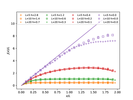
Figure 4: Normalized weight functions $J(x)/L$ determining the EH for different values of $\lambda=2hL$. Continuous lines correspond to the theoretical prediction, Eq. (39). The purple straight line corresponds to the Bisognano-Wichmann prediction for a semi-infinite system.

III Out of criticality

Let us consider an inhomogeneous ITF model described by the Hamitonian Eq. (2) or, equivalently, Eq. (4), with a modification of the coupling constants Eq. (5) studied in the previous section,

$$J_{m} = \begin{cases}e^{-2h|m+1/2|+\delta}&\text{if }m\neq-1/2,\\ e^{-h/2+\delta}&m=-1/2,\\ \end{cases}$$ (40)

$$\Gamma_{m} = e^{-2h|m|-\delta},$$ (41)

where $\delta\in\mathbb{R}$. Notice that if $h=0$ and $\delta\ll 1$, then $J_{m}=1+\delta$ and $\Gamma_{m}=1-\delta$, and our system describes a Majorana chain with alternating couplings, thus showing a relation to the Kitaev chain and the Su-Schrieffer-Heeger (SSH) model describing a dimerized chain of Dirac fermions Su.79 ; Heeger.88 . Indeed, the parity term $e^{\pm\delta}$ pushes the system described in Sec. II out of criticality, as we will describe throughout this section.

III.1 Strong Inhomogeneity

Let us consider the Hamiltonian given in Eq. (4) in the limit $h\gg 1$. We can apply the same SDRG of the previous section, making use of the parameter

$$\kappa=\delta/h.$$ (42)

The RS is obtained when all the RG steps decimate the Majoranas at the center of the chain, but we will show that other structures may be obtained, depending on the value of $\kappa$. In order to decimate the central pair we need $J_{1/2}$ to be the strongest coupling of the chain. In other words, $J_{-1/2}>\Gamma_{1/2}$ which implies that $e^{-h(1/2-\kappa)}>e^{-h(1+\kappa)}$. Hence, we arrive at the condition

$$\frac{1}{2}-\kappa<1+\kappa\Rightarrow\kappa>-\frac{1}{4}.$$ (43)

Thus, if $\kappa>-1/4$ the Majorana fermions $\beta_{-1/2}$ and $\alpha_{1/2}$ fuse into the Dirac fermion $b_{1/2}$, defined in Eq. (9) and, using Eq. (7), we obtain a renormalized coupling

$$\tilde{\Gamma}_{1/2}=e^{-3h\left(\frac{1}{2}+\kappa\right)},$$ (44)

which will couple $\alpha_{-1/2}$ and $\beta_{1/2}$. These Majorana fermions are decimated at the second RG step fusing into $d_{1/2}$, Eq. (11), if $\tilde{\Gamma}_{1/2}>J_{1/2}$, implying that

$$3\left(\frac{1}{2}+\kappa\right)<2-\kappa\Rightarrow\kappa<\frac{1}{8},$$ (45)

and then a new term appears in the effective Hamiltonian of the form $\tilde{J}_{3/2}\beta_{-3/2}\alpha_{3/2}$, where $\tilde{J}_{3/2}$ follows from Eq. (6),

$$\tilde{J}_{3/2}=e^{-5h\left(\frac{1}{2}-\kappa\right)}.$$ (46)

Summarizing, the first central decimation requires $\kappa>-1/4$ while the second requires $\kappa<1/8$. We can iterate this procedure and find that the bound on $\kappa$ associated to exactly $n$ consecutive central decimations is given by

$$\kappa >-\frac{1}{4n},\text{ if $n$ odd,}$$

$$\kappa <\frac{1}{4n},\text{ if $n$ even.}$$ (47)

The state with exactly $n$ central decimations will be called $\ket{n}$. With this notation, the RS corresponds to $\ket{n=2L}$, and satisfies

$$|\kappa|<\frac{1}{8L}.$$ (48)

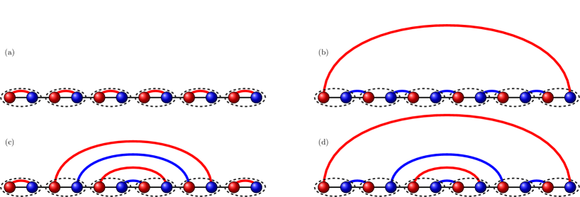
Figure 5: Schematic representation of different ground states of Eq. (4) obtained with the SDRG scheme. The trivial (a) and non-trivial (b) local pairings correspond to the states $\ket{n=0}$ and $\ket{n=1}$, the two possible ground states of the Kitaev chain. Panels (c) and (d) illustrate ground states with a coexistence between non-local rainbow-like and local fermions. The topological type of the local pairing depends on the parity of $n$. Hence, we have a trivial pairing (c) $\ket{n=4}$ and a non trivial one $\ket{n=3}$ in (d).

Whenever a central decimation fails, the SDRG must choose the strongest couplings between two identical links, symmetrically placed with respect to the center of the chain. That is not a problem for the algorithm, because the links are not consecutive Samos.20 . More relevantly, from that moment on the RG will always proceed by dimerizing the chain towards the extremes, except perhaps for a final long distance bond, depending on the parity of the system, related to the Kitaev phase Kitaev.01 .

Thus, we are led to the following physical picture, which is illustrated in Fig. 5. In panel (a) we can see the GS for $\kappa<-1/4$. No central bonds are created, and we obtain the state $\ket{n=0}$. Panel (b) shows the GS for $\kappa>1/8$, in which a single central bond is created. Due to parity reasons, a second bond must appear between the extremes of the chain, thus leading to the non-trivial Kitaev chain, which we call the state $\ket{n=1}$. Panel (c) shows the state $\ket{n=4}$ and panel (d) the state $\ket{n=3}$, which can be obtained within fixed ranges of $\kappa\in(-1/12,-1/20)$ and $\kappa\in(1/24,1/16)$ respectively, which can be found through Eq. (47).

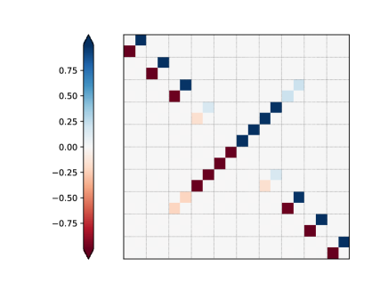
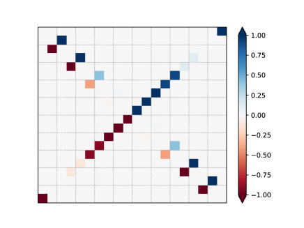
Figure 6: Covariance matrices of states $\ket{n=4}$ and $\ket{n=5}$ for $h=10$ and $N=20$. The short-range single states populate the secondary diagonals while the long-range singlet states correspond to the antidiagonal.

This physical picture can be confirmed through the analysis of the covariance matrices, which are depicted using a color code in Fig. 6. Indeed, we can see the CM for $N=20$ spins and $h=10$, in the suitable range for $\ket{n=4}$ (left) and $\ket{n=5}$ (right). The central patterns show $n=4$ and $n=5$ central arcs, respectively. As predicted, the $n=5$ case presents an extra bond between the extremes of the system, showing that it belongs to the non-trivial Kitaev phase.

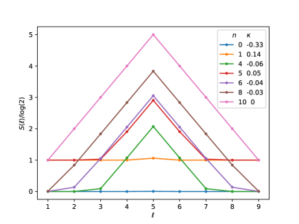
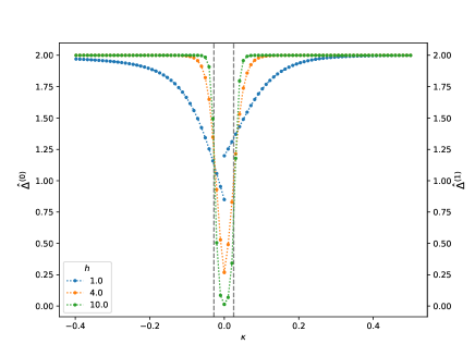
Figure 7: Top: EE of lateral blocks of a chain of $N=10$ spins for different values of $\kappa$, using $h=10$. For $\kappa=-0.33$ and $\kappa=0.14$ we obtain respectively the $\ket{n=0}$ and $\ket{n=1}$ states, for which the entropy is flat. On the other extreme, the $\kappa=0$ curve corresponds to the rainbow state, $\ket{n=10}$, which presents maximal EE growth. The intermediate values of $\kappa$ are chosen following Eq. (47) and present different numbers of central bonds. The EE for the half-chain, $\ell=5$, agrees with Eq. (19). Bottom: scaled energy gaps ($\hat{\Delta}^{(0)}$ for $\kappa<0$ and $\hat{\Delta}^{(1)}$ for $\kappa>0$) of the same chain for different values of $h$. The vertical gray lines delimit the rainbow state region for this chain size ($n>2(L-1)$).

Furthermore, we examine the EE of lateral blocks, $S(A_{\ell})$ in the top panel of Fig. 7, which has been computed from the CM using the same systems, with $N=10$ spins and $h=10$. As predicted in our physical picture, the EE for the smallest block begins at 0 or $\log(2)$ depending on the sign of $\kappa$, and presents a linear tent-shape at the center, within a block of $\lfloor n/2\rfloor$ spins and reaching an EE $n\log(2)/2$. The topological nature of the states is clarified in Appendix F, where we present a graphical way to distinguish the trivial and topological phases by overlaying each state with the trivial state $\ket{n=0}$ and counting the total number of loops.

We can also consider the energy gap around the Fermi level to capture the differences between ground states. Defining the energy gap in an inhomogeneous system presents some challenges, since it should be expressed in units of the typical energy scale. A strategy that has proved useful in similar cases is to rescale the energy gap with the lowest coupling of the system Samos.20 , which in this case becomes $\Gamma_{L-1/2}\approx e^{-2hL}$. Hence, the scaled gap

$$\hat{\Delta}^{(0)}\equiv\frac{E_{N+1}-E_{N}}{\Gamma_{L-{1/2}}},$$ (49)

becomes constant ($\hat{\Delta}^{(0)}=2$), as it can be seen in Fig.7 (b). The states $\ket{n\text{ odd}}$ present a zero mode at the edge, and the system is strictly gapless, $\hat{\Delta}^{(0)}=0$. Therefore, it is convenient to consider the second gap, defined as

$$\hat{\Delta}^{(1)}\equiv\frac{E_{N}-E_{N-1}}{J_{L-{1/2}}},$$ (50)

which can also be seen in Fig. 7 (b). If $n\leq(2L-3)$ there is a short-range Majorana singlet state and the gap is finite, $\hat{\Delta}^{(1)}=2$. Yet, both gaps fall to zero for the rainbow state, $\ket{n=N}$.

III.2 Weak Inhomogeneity

Proceeding in the same way as in the previous section, we can obtain the equations of motion from the Hamiltonian Eq. (4) and describe the continuum limit defining $x=am$, $a\to 0$, $h\to 0$, with $\hat{h}=h/a$ and $\mathcal{L}=La$ kept constant, in terms of the fields $\alpha(x,t)$ and $\beta(x,t)$,

$$\partial_{t}\alpha \approx-2ae^{-2\hat{h}|x|}\Bigl{(}ae^{\delta}\partial_{x}-\Bigl{(}\operatorname{sign}(x)he^{\delta}+2\sinh\delta\Bigr{)}\Bigr{)}\beta,$$

$$\partial_{t}\beta \approx-2ae^{-2\hat{h}|x|}\Bigl{(}ae^{\delta}\partial_{x}-\Bigl{(}\operatorname{sign}(x)he^{\delta}-2\sinh\delta\Bigr{)}\Bigr{)}\alpha,$$ (51)

where we will use $a=1$ for convenience. These equations can be rewritten in terms of a spinor field $\Psi$, Eq. (24), using the same $\gamma$ matrices, obtaining

$$\Bigl{(}-\sigma_{2}\partial_{0}+e^{-2h|x^{1}|}\bigl{(} i\sigma_{3}e^{\delta}\partial_{1}$$

$$-i\sigma_{3}\text{sign}(x^{1})he^{\delta}+2i\sinh\delta\bigr{)}\Bigr{)}\Psi=0,$$ (52)

And, then, we can compare this equation with that representing the dynamics of a Dirac field in a curved space time.

$$\left(-\sigma_{2}\partial_{0}+\frac{i}{2}\omega_{0}^{01}\sigma_{3}+\frac{E_{1}^{1}}{E_{0}^{0}}\left(i\sigma_{3}\partial_{1}-\frac{i}{2}\omega_{1}^{01}\sigma_{2}\right)+i\frac{m}{E_{0}^{0}}\right)\Psi=0.$$ (53)

where $\omega^{ab}_{\mu}$ is again the spin connection and $E^{\mu}_{a}$ the inverse of the zweibein. From the above identification we find that:

$$E^{0}_{0} = e^{2h|x^{1}|},\quad E^{1}_{1}=e^{\delta}$$

$$\omega^{01}_{0} = -2e^{-2h|x^{1}|}e^{\delta}h\text{sign}(x^{1})$$

$$\omega^{01}_{1} = 0,$$

$$m = 2\sinh\delta,$$ (54)

that leads to a (1+1)D metric whose non-zero terms are

$$g_{00}=-e^{-4h|x|},\qquad g_{11}=e^{-2\delta}.$$ (55)

However, $g_{11}\simeq 1$ if $\delta\ll 1$, and thus the associated metric coincides with the one found in the previous section, see Eq. (31). Thus, the field theory associated to the system described by the Hamiltonian (4) is described by a massive Majorana fermion, with $m\approx 2\delta$, placed in the curved background described by the metric Eq. (31).

III.2.1 Entanglement entropies

Let us first consider the case $h=0$, i.e. the massive fermion on a flat space. The EE of this system has been obtained previously by evaluating the associated two-dimensional classical model via the CTM formalism Peschel.09 . For $\delta>0$ one obtains

$$S(\delta)=\frac{1}{12}\left(\log\left(\frac{k^{2}}{16k^{\prime 2}}\right)+\left(1-\frac{k^{2}}{2}\right)\frac{4I(k)I(k^{\prime})}{\pi}\right)+\log 2,$$ (56)

while for $\delta<0$ we get

$$S(\delta)=\frac{1}{12}\left(\log\left(\frac{4}{kk^{\prime}}\right)+\frac{1}{2}\left(k^{2}-k^{\prime 2}\right)\frac{4I(k)I(k^{\prime})}{\pi}\right),$$ (57)

where $I(x)$ is the complete elliptic integral of the first kind Abramowitz and

$$k=e^{-2|\delta|},\qquad k^{\prime}=\sqrt{1-k^{2}}.$$ (58)

Notice that if $|\delta|\ll 1$, $k\approx(1-|\delta|)/(1+|\delta|)$ which is the value used in Refs. Peschel.09 ; Eisler.20 . Although Eq. (57) is only exact for the infinite chain, it is still valid provided that $1/\delta\ll L$, i.e. when the cluster decomposition principle is satisfied. Near the critical point, $\delta\ll 1$, Eqs. (57) are simplified to

$$S\approx\frac{c}{6}\log(\frac{1}{1-k})=\frac{c}{6}\log\xi,$$ (59)

where the quantity inside the logarithm can be interpreted as a correlation length $\xi$ Calabrese.04 with the appropriate units of length,

$$\xi=\frac{1}{1-k}\approx\frac{1}{2|\delta|},$$ (60)

which corresponds to the inverse of the mass, $m=2\delta$, Eq. (54). To end this brief summary of the homogeneous non critical case, let us write the EE for the half chain of a finite system as

$$S(\delta,L)=\frac{c}{6}\log\frac{\xi_{E}(\delta,L)}{2}+b(\delta),$$ (61)

where $\xi_{E}(\delta,L)$ shall be called the entanglement length, because it plays the role of an effective correlation length in order to compute the EE, even though its value is upper bounded by the size of the system, $N=2L$. If $\delta=0$, the system is critical and $\xi_{E}(0,L)$ saturates this bound, thus leading to the logarithmic scaling predicted by CFT. On the other hand, if $|\delta|$ is large enough then $\xi_{E}(\delta,L)\ll 2L$, finite size effects are not important and the cluster decomposition principle holds. Thus, the results for the infinite chain can be applied, and the area law is satisfied. Hence, we see that in this case Eq. (61) is just a reparametrization of Eq. (57).

Moreover, when we introduce inhomogeneity in the system through the parameter $h$, we find that the EE can be obtained merely deforming the entanglement length $\xi_{E}(\delta,L)$ according to the same prescription used before, given in Eq. (32), giving rise to the Ansatz

$$S(L,\delta,h)=\frac{c}{6}\log\left(\tilde{\xi}_{E}(\delta,L)\right)+b(\delta),$$ (62)

where

$$\tilde{\xi}_{E}(h,\delta,L)=\frac{1}{2h}\left(e^{h\xi_{E}(\delta,L)}-1\right),$$ (63)

is the deformed entanglement length, corresponding to the curved space-time.

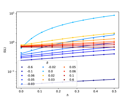
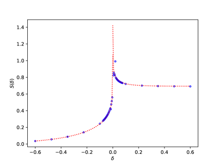
Figure 8: Top: Plot of the fits (lines) performed with expression (63) of the numerical results for the half chain EE (points) for different values of $\delta$. Bottom: The dotted red line corresponds to Eq. (57) and the blue dots to Eq. (62), where $\xi_{E}(\delta,L)$ has been obtained by fitting Eq. (63) to the numerical half chain EE of a system with $L=100$.

We have fitted expression Eq. (62) to the numerical values for the EE of the half chain for different values of $\delta$ and $h$, using $\xi_{E}(\delta,L)$ and $b(\delta)$ as fitting parameters. The agreement between the fits and the numerical results can be seen in the top panel of Fig. 8. Hence, we obtain a single value for the entanglement length for each $L$ and $\delta$, which accounts for the EE under different degrees of inhomogeneity $h$. In the bottom panel of Fig. 9 we can see the good agreement between the infinite chain prediction, Eq. (57), and the output of Eq. (61) having used the values $\xi_{E}(\delta,L)$ and $b(\delta)$ that were obtained from the previous fits.

In Fig. 9 we present the fitted values $\xi_{E}(\delta,L)$ for different system sizes. The system presents universal behavior as long as the correlation length is much smaller than the system size.

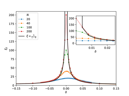
Figure 9: Entanglement correlation length $\xi_{E}(\delta,L)$ for different chain sizes $2L$. Near the critical point we have $\xi_{E}\approx\xi$, Eq. (60).

It is worth to ask whether the weak and strong inhomogeneity regimes match smoothly. Let us consider the limit $h\gg 1$ in Eq. (62),

$$S(L,\delta,h)\approx\frac{c}{6}h\xi_{E}(\delta,L).$$ (64)

If $\delta=0$ we have $S(L,0,h)\approx\frac{c}{3}hL$, as it was discussed in the previous section. On the other hand, if $\delta\ll 1$ but $1/\delta\ll L$, $\xi_{E}(\delta,L)=\xi$ from Eq. (60). Hence,

$$S(L,\delta,h)\approx\frac{h}{12\delta}=\frac{1}{12\kappa},$$ (65)

which is a manifestation of the area law given by the interplay between the inhomogeneity $h$ and the dimerization $\delta$. Thus, we see that the weak and strong inhomogeneity regimes match.

III.2.2 Entanglement Hamiltonian and Entanglement Spectrum

The reduced density matrix $\rho_{A}$ of a half infinite chain can be written in terms of the generator of the Baxter corner matrix,

$$\rho_{A}=e^{-H_{CTM}},$$ (66)

Since the model is integrable, we can simplify and state that $H_{CTM}=\epsilon H_{\mathcal{N}}$, where $H_{\mathcal{N}}$ is a Hermitian operator with integer spectrum. Thus, the ES $\epsilon_{l}$, with $l=1\dots L$, is equally spaced and we may focus on the level spacing $\epsilon$. For the ITF model we have

$$\epsilon=\pi\frac{I(k^{\prime})}{I(k)},$$ (67)

where $k$ and $k^{\prime}$ are given by Eq. (58). The EH of the half infinite chain can be identified with the generator of the CTM Eisler.20 . Thus, in the case of the ITF chain the first neighbor couplings grow linearly from the internal boundary towards the bulk with a parity oscillation between $1$ and $k$,

$$\mathcal{H}=\sum_{l=1}^{\infty}J^{EH}_{2\ell-1}\alpha_{\ell}\beta_{\ell}+J^{EH}_{2\ell}\beta_{\ell}\alpha_{\ell+1},$$ (68)

with

$$\displaystyle J^{EH}_{2\ell-1}=I(k^{\prime})(2\ell-1),\quad J^{EH}_{2\ell}=I(k^{\prime})2\ell k,\quad\delta<0$$

$$\displaystyle J^{EH}_{2\ell-1}=I(k^{\prime})(2\ell-1)k,\quad J^{EH}_{2\ell}=I(k^{\prime})2\ell,\quad\delta>0$$ (69)

where $\alpha_{\ell}$ and $\beta_{\ell}$ correspond to the lattice Majorana fermions. Fig. 10 (a) shows the nearest neighbor coupling constants of the EH, $J^{EH}_{\ell}$, slightly modified in order to improve the visualization: for odd values of $\ell$, $J^{EH}_{\ell}$ has been divided by $k$ in order to remove the parity oscillation, leaving a linear growth with slope $2I(k^{\prime})$, in similarity to Eisler.20 . If we switch on the inhomogeneity, setting $h=0.5$, we can observe the same EH couplings in Fig. 10 (b): a linear increase of the couplings with a parity oscillation beween values $1$ and $\hat{k}(h)$, which depends on the inhomogeneity. Notice that $\hat{k}(0)=k$.

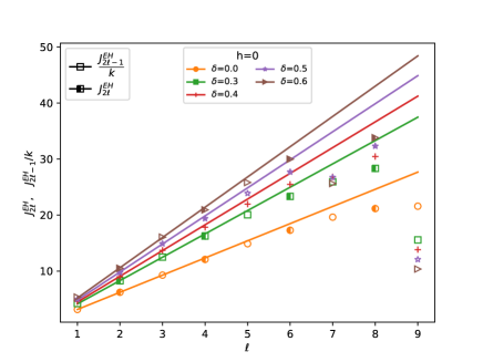
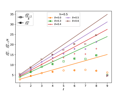
Figure 10: Nearest neighbor couplings of a chain of $2N=20$ Majorana fermions, $J^{EH}_{\ell}$, with a parity compensation: odd values of $\ell$ are divided by $k$. (a) Case $h=0$. We can see that, despite the small size of the chain, we recover the behaviour of the infinite chain near the boundary for strong dimerizations. Empty symbols correspond to even couplings while the filled ones are for $J^{EH}_{2\ell-1}/k$, see Eq. 69. (b) In the case $h=0.5$ we observe the same initial behavior for low values of $\ell$.

IV Conclusions and further work

In this work we have characterized the entanglement properties of an inhomogeneous transverse field Ising critical spin-1/2 chain for which both the couplings and external fields fall exponentially from the center with a rate $h$, which defines the rainbow ITF model. It can be analytically solved by mapping into a Majorana chain, which suggests to treat the couplings and the external fields on an equal footing. Applying the strong disorder renormalization method we find that the ground state can be expressed in terms of generalized singlet states which are displayed concentrically around the center, similarly to the rainbow state. The weak inhomogeneity regime can be characterized by taking the continuum limit and showing that the resulting field theory corresponds to a free massless Majorana fermion field on a curved space-time. Thus, we are able to predict the behavior of the entanglement entropy deforming appropriately the known CFT results for Minkowski space-time, which turns the characteristic logarithmic growth into a linear growth with the block size. Moreover, there is a smooth crossover between both regimes. The nearest neighbor coefficients of the entanglement Hamiltonian present the standard linear growth as we move away from the internal boundary, in agreement with the Bisognano-Wichmann theorem, showing that the state can be interpreted as a thermofield double for large enough inhomogeneity.

Out of criticality, we introduce a parity-dependent term whose strength $\delta$ competes with $h$, attempting to destroy the linear entanglement. Strong-disorder renormalization arguments show that for each value of $\kappa\equiv\delta/h$ we obtain a fixed number of concentric singlets around the center of the chain, also showing that the trivial and non-trivial Kitaev phases are obtained for positive and negative values of $\kappa$, although with a substantial deformation. The weak inhomogeneity regime with small $\delta$ is described by a massive Majorana field theory placed over the curved space-time that we found in the case of the critical model. We have computed the EE by defining an effective correlation length $\xi_{E}(\delta,L)$ which is deformed with the metric, see Eq. (61). Near the entangling point, the entanglement Hamiltonian presents a linear growth of the couplings with a parity oscillation that can be accounted for using CTM results for the infinite systems. The amplitude of the oscillation and the slope depends on the inhomogeneity parameter.

In a previous work Samos.19 , we found a connection between the rainbow antiferromagnetic Heisenberg spin chain with the Haldane phase, and another between the rainbow XX spin chain and the BDI SPT phases, by means of a folding transformation around the center of the symmetry of the chain. It could be interesting to extend this approach to the models considered in this manuscript and, more generally, to address the entanglement characterization of inhomogeneous 2D systems. In addition, it could be relevant to consider an experimental realization of the rainbow state in terms of a Rydberg atoms chain whose effective Hamiltonian is an inhomogeneous ITF model with an additional longitudinal field Schauss.18 . It is possible to extend Fisher’s RG to this model and find the conditions under which a rainbow is formed. Also, it could be interesting to consider strongly inhomogeneous anyon models and study them harnessing their relation with $SU(2)_{k}$ Chern-Simons theories Bonesteel.07 ; Nayak.08 .

Appendix A SDRG on Majorana chains

In this appendix we explain the SDRG scheme applied to an inhomogeneous chain of Majorana fermions. Let us consider a system of $4$ Majorana fermions whose Hamiltonian is given by:

$$H=i\left(g_{ia}\gamma_{i}\gamma_{a}+g_{ib}\gamma_{i}\gamma_{b}+g_{ab}\gamma_{a}\gamma_{b}+g_{aj}\gamma_{a}\gamma_{j}+g_{bj}\gamma_{b}\gamma_{j}\right),$$ (70)

with $\{\gamma_{m},\gamma_{n}\}=2\delta_{mn}$. Let us assume that $g_{ab}$ is larger than the rest so we can use use perturbation theory to diagonalize (70).

$$H_{0} =ig_{ab}\gamma_{a}\gamma_{b},$$ (71)

$$H_{I} =i\left(g_{ia}\gamma_{i}\gamma_{a}+g_{ib}\gamma_{i}\gamma_{b}-g_{ja}\gamma_{j}\gamma_{a}-g_{jb}\gamma_{j}\gamma_{b}\right)\ .$$ (72)

Defining the Dirac fermion $b=\frac{1}{2}\left(\gamma_{a}+i\gamma_{b}\right)$, we have that $H_{0}=2g_{ab}\left(b^{\dagger}b-1/2\right)$ whose spectrum is $\pm|g_{ab}|$ and eigenvectors $\ket{0},\ket{1}$ such that $b\ket{0}=0$. The $H_{I}$ can be written as:

$$H_{I}=i\left\{\left[\left(g_{ia}-ig_{ib}\right)\gamma_{i}-\left(g_{aj}-ig_{bj}\right)\gamma_{j}\right]b+\left[\left(g_{ia}+ig_{ib}\right)\gamma_{i}-\left(g_{aj}+ig_{bj}\right)\gamma_{j}\right]b^{\dagger}\right\}$$ (73)

Note that we must extend the Hilbert space: $\ket{0}\to\ket{0}\otimes\ket{\psi}$ where $\ket{\psi}$ is an unknown state of the Majorana fermions $\gamma_{i},\gamma_{j}$. In the same way $\ket{1}\to\ket{1}\otimes\ket{\varphi}$. However we shall make an abuse of notation and write $\gamma_{i}$ instead of $\langle\psi|\gamma_{i}|\varphi\rangle$. The first order corrections are zero so we compute the second order:

$$\Delta E_{0}=\frac{\langle 0|H_{I}|1\rangle\langle 1|H_{I}|0\rangle}{E_{0}-E_{1}}.$$ (74)

Using Eq. (73) we find the same corrections for $g_{ab}>0$ and $g_{ab}<0$

$$\Delta E_{0}=i\left(\frac{g_{ia}g_{bj}}{g_{ab}}-\frac{g_{ib}g_{aj}}{g_{ab}}\right)\gamma_{i}\gamma_{j}+\tilde{E},$$ (75)

with $\tilde{E}_{0}=1/(2|g_{ab}|)\left(g_{ia}^{2}+g_{ib}^{2}+g_{bj}^{2}+g_{aj}^{2}\right)$. Thus, an effective Hamiltonian $H_{eff}=ig_{ij}\gamma_{i}\gamma_{j}$ emerge with the hopping term given by

$$g_{ij}=\frac{g_{ia}g_{bj}}{g_{ab}}-\frac{g_{ib}g_{aj}}{g_{ab}}.$$ (76)

Particularizing for the ITF spin chain, $g_{ib}=g_{aj}=0$ and we recover Eq. (6) and (7). In Ref. Bonesteel.07 the authors provide the same result with a graphical derivation. The matrix elements are computed by counting the loops obtained by overlaying the (generalized) singlet states. See Appendix F for details of the overlaying procedure.

Appendix B Covariance Matrices

Let us consider a system of $N=2L$ Majorana fermions given by the quadratic Hamiltonian:

$$\mathcal{H}=i\bm{\gamma}^{T}A\bm{\gamma},$$ (77)

where $\bm{\gamma}^{T}=(\gamma_{1}\dots\gamma_{N})$ and $A=-A^{T}$. There exists a transformation $Q\in SO(2N)$ which brings the Hamiltonian to the canonical form

$$Q^{T}AQ=N_{\epsilon},$$ (78)

where $N_{\epsilon}$ is a block diagonal matrix

$$N_{\epsilon}=\left(\begin{array}[]{c|c}0&\bm{\epsilon}\\ \hline\cr-\bm{\epsilon}&0\end{array}\right),$$ (79)

where $\bm{\epsilon}$ is an $L\times L$ matrix with $\text{diag}(\bm{\epsilon})=(\epsilon_{1},\dots,\epsilon_{L})$, which are the positive eigenvalues of the matrix $iA$. We have then that

$$\mathcal{H}=i\bm{\gamma}^{T}A\bm{\gamma}=i\bm{\gamma}^{T}QN_{\epsilon}Q^{T}\bm{\gamma}=i\tilde{\bm{\gamma}}^{T}N_{\epsilon}\tilde{\bm{\gamma}},$$ (80)

where we have defined a set of Majorana fermions $\tilde{\bm{\gamma}}=Q^{T}\bm{\gamma}$. These Majorana fermions can be arranged into Dirac fermions $\bm{\Psi}^{T}=(\bm{b},\bm{b}^{\dagger})=(b_{1}\dots b_{L},b^{\dagger}_{1}\dots b_{L}^{\dagger})$ with $\bm{\Psi}=U\tilde{\bm{\gamma}}$ and

$$U=\left(\begin{array}[]{c|c}\mathbb{I}&i\mathbb{I}\\ \hline\cr\mathbb{I}&-i\mathbb{I}\end{array}\right),$$ (81)

where $\mathbb{I}$ is the $L\times L$ identity matrix. The Hamiltonian takes the form $\mathcal{H}=\sum_{k}\epsilon_{k}(b^{\dagger}_{k}b_{k}-1)$ and the correlators are particularly simple,

$$\expectationvalue{\bm{\Psi}\bm{\Psi}^{\dagger}}=\left(\begin{array}[]{c|c}\mathbb{I}&0\\ \hline\cr 0&0\end{array}\right).$$ (82)

We can express it back in terms of the Majorana fermions $\expectationvalue{\bm{\Psi}\bm{\Psi}^{\dagger}}=U\expectationvalue{\tilde{\bm{\gamma}}\tilde{\bm{\gamma}}^{T}}U^{\dagger}$ and those in terms of the physical Majorana fermions $\bm{\gamma}$,

$$\expectationvalue{\bm{\gamma}\bm{\gamma}^{T}}=Q^{T}\left(\begin{array}[]{c|c}\mathbb{I}&i\mathbb{I}\\ \hline\cr-i\mathbb{I}&\mathbb{I}\end{array}\right)Q.$$ (83)

The symmetric part of the matrix above is given by the anticommutation relation of the Majorana fermions, while the antisymmetric part that contains all the non-trivial information is known as the covariance matrix.

Appendix C Dirac Fermion in Curved Spacetime

Let us consider the Dirac equation in curved spacetime:

$$(i\not{D}-m)\Psi=0,$$ (84)

where $\not{D}=E^{\mu}_{a}\gamma^{a}D_{\mu}$ is the slashed covariant derivative, and $E^{\mu}_{a}=g^{\mu\nu}\eta_{ab}e^{b}_{\nu}$ is the inverse of the tetrad basis (or zweibein) $e^{a}_{\mu}$ that satisfies $g_{\mu\nu}=e^{a}_{\mu}e^{b}_{\nu}\eta_{ab}$. More precisely, the covariant derivative of the two component spinor $\Psi$ is given by

$$D_{\mu}\Psi=\left(\partial_{\mu}-\frac{1}{8}\omega^{ab}_{\mu}[\gamma_{a},\gamma_{b}]\right)\Psi,$$ (85)

where $\omega^{ab}_{\mu}$ is the spin-connection which is defined in terms of the Christoffel symbols $\Gamma^{\nu}_{\sigma\mu}$ and the inverse of the tetrad $E^{\mu}_{a}$,

$$\omega^{ab}_{\mu}=e^{a}_{\nu}\partial_{\mu}E^{b\nu}+e^{a}_{\nu}E^{b\sigma}\Gamma^{\nu}_{\sigma\mu},$$ (86)

As we are considering a static system, it is reasonable to assume that the tetrad matrix $e^{a}_{\mu}$ is diagonal ($E_{0}^{1}=E_{1}^{0}=0$). Expanding (84) with this assumption leads to

$$\left(iE_{0}^{0}\gamma^{0}\left(\partial_{0}-\frac{1}{8}\omega_{0}^{ab}[\gamma_{a},\gamma_{b}]\right)+iE_{1}^{1}\gamma^{1}\left(\partial_{1}-\frac{1}{8}\omega_{0}^{ab}[\gamma_{a},\gamma_{b}]\right)-m\right)\Psi=0\ .$$ (87)

Taking in account that $[\gamma_{0},\gamma_{1}]=[-\gamma^{0},\gamma^{1}]=-2\gamma^{3}$ and the antisymmetry of the internal indices of the spin connection we arrive at

$$\left(\gamma^{0}\partial_{0}+\frac{1}{2}\omega_{0}^{01}\gamma^{0}\gamma^{3}+\frac{E_{1}^{1}}{E_{0}^{0}}\left(\gamma^{1}\partial_{1}+\frac{1}{2}\omega_{1}^{01}\gamma^{1}\gamma^{3}\right)+i\frac{m}{E_{0}^{0}}\right)\Psi=0\ .$$ (88)

Appendix D Non universal function of the EE

The relation between the entanglement entropies of the XX and ITF models is given by Igloi.08 :

$$S_{\text{XX}}(2x,2L)=2S_{\text{ITF}}(x,L).$$ (89)

We will compute the non universal part of the EE (36) with the above expression. The EE of the XX model whose ground state is a RS has been studied in the past Laguna.17b ,

$$S_{XX}(2x,2L) = S_{cft}(2x,2L)+\frac{\gamma_{1}}{2}+S_{oscl}(2x,2L),$$ (90)

$$S_{cft}(2x,2L) = \frac{1}{6}\log\left(e^{-h|2x|}\frac{8(e^{h2L}-1)}{h\pi}\cos(\frac{\pi(e^{h|2x|}-1)}{2(e^{h2L}-1)})\right)$$

$$S_{oscl}(2x,2L) = (-1)^{2x+2L}\left(\frac{8(e^{h2L}-1)}{h\pi}\cos\left(\frac{\pi(e^{h|2x|}-1)}{2(e^{h2L}-1)}\right)\right)^{-1},$$

and $\gamma_{1}\approx 0.4950+1/3\log 2$ Jin.04 . Hence, by using relation Eq. (89) we have

$$c^{\prime}_{I}(x,L) = \frac{\gamma_{1}}{4}+\frac{1}{6}\log 2+$$ (91)

$$(-1)^{L} \left(\frac{16(e^{2hL}-1)}{h\pi}\cos\left(\frac{\pi(e^{2h|x|}-1)}{4(e^{2hL}-1)}\right)\right)^{-1}.$$

Appendix E Computation of the Entanglement Hamiltonian

The entanglement Hamiltonian can be obtained by knowing the covariance matrix. Consider a system of $N=2L$ Majorana fermions given by the quadratic Hamiltonian Eq. (77). There exists a transformation $O\in SO(2N)$ which brings the Hamiltonian to the canonical form $O^{T}AO=N^{\prime}_{\epsilon}$, where $N^{\prime}_{\epsilon}$ is a block diagonal matrix

$$N^{\prime}_{\epsilon}=\bigoplus_{k}^{L}\left(\begin{matrix}0&\epsilon_{k}\\ -\epsilon_{k}&0\end{matrix}\right),$$ (92)

where $\pm\epsilon_{k},k=1\dots L$ are the eigenvalues of the matrix $iA$. Notice that $N^{\prime}_{\epsilon}$, Eq. (92), and $N_{\epsilon}$, Eq. (79), are similar matrices meaning that $O$ and $Q$ differ in the order of the elements of the basis. The transformation $O$ is more convenient because the lateral blocks considered in the main text are contiguous in this basis. Thus, the Hamiltonian reads also as Eq. (80) after substituting $Q$ by $O$. The density matrix $\rho$ associated to the the GS of a quadratic Hamiltonian can always be written as

$$\rho=\mathcal{K}e^{\mathcal{-H}},$$ (93)

where $\mathcal{K}$ is a normalization constant and $\mathcal{H}$ is called the entanglement Hamiltonian (EH), given by (77). It is possible to obtain $\mathcal{H}_{A}$, the EH associated to the reduced density matrix $\rho_{A}$ by knowing the associated partial covariance matrix $\mathcal{C}_{A}=\expectationvalue{\gamma_{i}\gamma_{j}}$ with $i,j\in A$.

$$\mathcal{C}_{A}=O^{T}N^{\prime}_{\lambda}O,$$ (94)

$N^{\prime}_{\lambda}$ has the same structure as $N^{\prime}_{\epsilon}$ but contains the eigenvalues of $\mathcal{C}_{A}$. Since the matrix $O$ brings to the normal form both $\mathcal{C}_{A}$ and $\mathcal{H}_{A}$, there is a relation between the eigenvalues of the EH $\epsilon$, known as entanglement spectrum (ES), and the eigenvalues of the covariance matrix:

$$\lambda_{k}=-\tanh\frac{\epsilon_{k}}{2}$$ (95)

Hence, by inverting the above relation, it is possible to compute the EH knowing the covariance matrix,

$$\mathcal{H}=O^{T}N^{\prime}_{\epsilon(\lambda)}O.$$ (96)

Appendix F Pictorial distinction of the topological phases

The trivial and topological ground states $\ket{n}$ of Eq. (4) can be distinguished graphically. We start by overlapping the GS with the trivial Majorana singlet state $\innerproduct{n}{n=0}$ and connecting the Majorana fermions (red and blue balls) with their opposites, leading to the formation of closed loops.

In Fig. 11 we show the same GS that we presented in Fig. 5 overlapping with $\ket{n=0}$, which we will call $\innerproduct{n=0}{n=0}$, that leads to $N$ loops matching with the $N$ Dirac fermions of kind $c$, see Eq. (3). This can be seen in panel $(b)$. On the other side, the overlapping $\innerproduct{n=1}{n=0}$ leads to just one big loop as it can be seen in panel $(c)$. Thus, the topological phase is characterized by a big loop that encloses all the Majorana fermions. Considering $1<n<L-2$ central decimations, the overlapping $\innerproduct{n=2m}{n=0}$ with $m=0,\cdots,L-1$ decreases the total number of loops to $N-m$ while the overlapping $\innerproduct{n=2m-1}{n=0}$ with $m=1,\cdots,L-1$ increases them up to $m$. For instance, in Fig. 11 $(d)$ we see the overlapping $\innerproduct{n=4}{n=0}$ that leads to $6-2=4$ bonds. In panel $(e)$ there are $2$ loops, because the overlapping corresponds to $\innerproduct{n=3}{n=0}$. Finally, as it can be seen in panel $(a)$, the overlaying of a rainbow state $\ket{\text{RS}}{n=0}$ leads to $N/2$ loops. This is another way of unveiling the criticality of the RS since it corresponds to the intermediate situation.

The loops can also be interpreted in terms of spins and Fisher’s RG Bonesteel.07 . Each loop contains those spins that were hybridized in consecutive RG steps with dominant $J$. Hence, the state $\ket{n=1}$ is a superspin while the RS can be seen as a collection of hybridized pairs of spins. However, notice that they do not form a singlet state as it is the case of the RS of the XX chain Eq. (15).

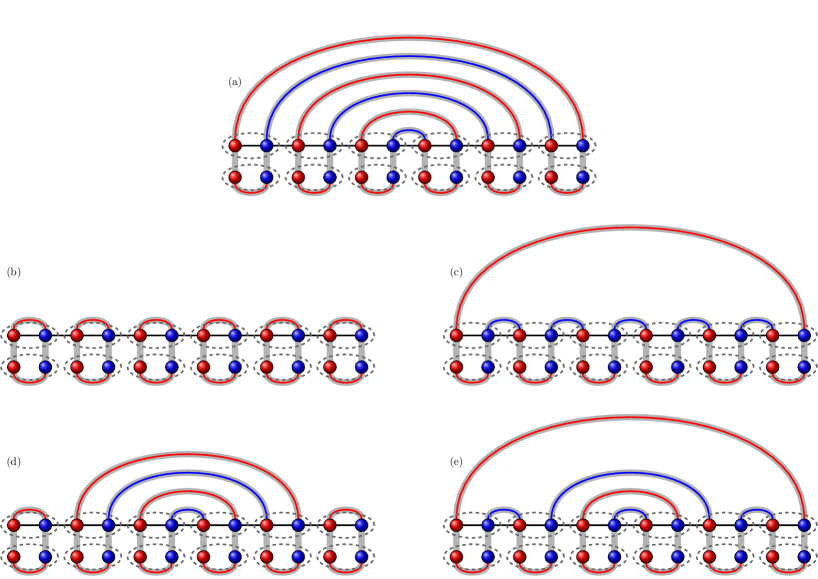
Figure 11: Overlapping of the same states considered in Fig. 5. Discussion on the main text.

References

- (1) L Amico, R Fazio, A Osterloh and V Vedral, Entanglement in many-body systems, Rev. Mod. Phys. 80, 517 (2008).
- (2) P. Calabrese, J. Cardy and B. Doyon, Entanglement entropy in extended quantum systems J. Phys. A: Math. Theor. 42 500301 (2009).
- (3) N Laflorencie, Quantum entanglement in condensed matter systems, Phys. Rep. 643, 1 (2016).
- (4) S. Singha Roy, S.N. Santalla, J. Rodríguez-Laguna and G. Sierra, Entanglement as geometry and flow, Phys. Rev. B 101, 195134 (2020).
- (5) B Zeng,X Chen, D L Zhou and X G Wen, Quantum information meets quantum matter. New York: Springer (2019).
- (6) M Sredniki, Entropy and area, Phys. Rev. Lett. 71, 666 (1993).
- (7) M.B. Hastings, Solving gapped Hamiltonians locally, Phys. Rev. B 73, 085115 (2006).
- (8) M.M. Wolf, F. Verstraete, M.B. Hastings and I. Cirac, Area laws in quantum systems: mutual information and correlations, Phys. Rev. Lett. 100, 070502 (2008).
- (9) J Eisert, M Cramer and MB Plenio,Area-laws for the entanglement entropy: a review,Rev. Mod. Phys. 82, 277 (2010).
- (10) C Holzhey, F Larsen and F Wilczek, Geometric and renormalized entropy in conformal field theory, Nucl. Phys. B 424, 443 (1994).
- (11) G Vidal, JI Latorre, E Rico and A Kitaev, Entanglement in quantum critical phenomena, Phys. Rev. Lett. 90 227902 (2003).
- (12) P Calabrese and JL Cardy, Entanglement entropy and quantum field theory, JSTAT P06002 (2004).
- (13) P Calabrese and J Cardy, Entanglement entropy and conformal field theory, J. Phys. A 42, 504005 (2009).
- (14) G Refael and JE Moore, Entanglement Entropy of Random Quantum Critical Points in One Dimension, Phys. Rev. Lett. 93,260602 (2004).
- (15) G Refael and JE Moore, Criticality and entanglement in random quantum systems, J. Phys. A 42, 504010 (2009).
- (16) N. Laflorencie, Scaling of entanglement entropy in the random singlet phase Phys. Rev. B 72, 140408 (2005).
- (17) M Fagotti, P Calabrese and JE Moore, Entanglement spectrum of random-singlet quantum critical points, Phys. Rev. B 83, 045110 (2011).
- (18) G Ramírez, J Rodríguez-Laguna and G Sierra, Entanglement in low-energy states of the random coupling model, JSTAT P07003 (2014).
- (19) P Ruggiero, V Alba and P Calabrese, The entanglement negativity in random spin chains, Phys. Rev. B 94, 035152 (2016).
- (20) M. Campostrini and E. Vicari, Quantum critical behavior and trap-size scaling of trapped bosons in a one-dimensional optical lattice Phys. Rev. A 81, 063614 (2010).
- (21) J. Dubail, J. M. Stephan, J. Viti and P. Calabrese, Conformal field theory for inhomogeneous one-dimensional quantum systems: the example of non-interacting Fermi gases SciPost Phys. 2, 002 (2017).
- (22) S. Murciano, P. Ruggiero and P. CalabreseEntanglement and relative entropies for low-lying excited states in inhomogeneous one-dimensional quantum systems J. Stat. Mech. 034001 (2019).
- (23) H. Ueda and T. Nishino, Hyperbolic Deformation on Quantum Lattice Hamiltonians J. Phys. Soc. Jpn. 78, 014001 (2009).
- (24) S. Sachdev and J. Ye, Gapless spin-fluid ground state in a random quantum Heisenberg magnet Phys. Rev. Lett. 70, 3339 (1993).
- (25) V. Rosenhaus, An introduction to the SYK model J. Phys. A: Math. Theor. 52 323001 (2019).
- (26) O. Boada, A. Celi, J.I. Latorre and M. Lewenstein, Dirac equation for cold atoms in artificial curved spacetimes, New J. Phys. 13, 035002 (2011).
- (27) J. Rodríguez-Laguna, L. Tarruell, M. Lewenstein and A. Celi, Synthetic Unruh effect in cold atoms, Phys. Rev. A 95, 013627 (2017).
- (28) B. Mula, S. N. Santalla, and J. Rodríguez-Laguna, Casimir forces on deformed fermionic chains, Phys. Rev. Research 3, 013062 (2021).
- (29) C. Dasgupta and S.-K. Ma, Low-temperature properties of the random Heisenberg antiferromagnetic chain, Phys. Rev. B 22, 1305 (1980).
- (30) G. Vitagliano, A. Riera and J. I. Latorre, Volume-law scaling for the entanglement entropy in spin 1/2 chains, New J. Phys. 12, 113049 (2010).
- (31) G. Ramírez, J. Rodríguez-Laguna and G. Sierra, From conformal to volume-law for the entanglement entropy in exponentially deformed critical spin 1/2 chains, J. Stat. Mech. P10004 (2014).
- (32) B. Alkurtass, L. Banchi and S. Bose, Optimal Quench for Distance-Independent Entanglement andMaximal Block Entropy, Phys. Rev. A 90, 042304 (2014).
- (33) G. Ramírez, J. Rodríguez-Laguna and G. Sierra, Entanglement over the rainbow, J. Stat. Mech. P06002 (2015).
- (34) J. Rodríguez-Laguna, S.N. Santalla and G. Ramírez, G. Sierra, Entanglement in correlated random spin chains, RNA folding and kinetic roughening, New J. Phys. 18, 073025 (2016).
- (35) J. Rodríguez-Laguna, J. Dubaîl, G. Ramírez, P. Calabrese and G. Sierra, More on the rainbow chain: entanglement, space-time geometry and thermal states, J. Phys. A 50, 164001 (2017).
- (36) E. Tonni, J. Rodríguez-Laguna and G. Sierra, Entanglement hamiltonian and entanglement contour in inhomogeneous 1D critical systems, J. Stat. Mech. 043105 (2018).
- (37) I. MacCormack, A.L. Liu, M. Nozaki and S. Ryu, Holographic Duals of Inhomogeneous Systems: The Rainbow Chain and the Sine-Square Deformation Model, J. Phys. A: Math. Theor. 52 505401 (2019).
- (38) N Samos Sáenz de Buruaga, S. N. Santalla, J Rodríguez-Laguna and G Sierra, Symmetry protected phases in inhomogeneous spin chains, JSTAT 093102 (2019).
- (39) N Samos Sáenz de Buruaga, SN Santalla, J Rodríguez-Laguna and G Sierra, Piercing the rainbow state: Entanglement on an inhomogeneous spin chain with a defect, Phys. Rev. B 101, 205121 (2020).
- (40) R.N. Alexander, A. Ahmadain, Z. Zhang and I. Klich, Exact rainbow tensor networks for the colorful Motzkin and Fredkin spin chains, Phys. Rev. B 100, 214430 (2019).
- (41) V. Alba, S. N. Santalla, P. Ruggiero, J. Rodríguez-Laguna, P. Calabrese and G. Sierra, Unsual area-law violation in random inhomogeneous systems, JSTAT 023105 (2019).
- (42) H. Li and F D M Haldane, Entanglement Spectrum as a Generalization of Entanglement Entropy: Identification of Topological Order in Non-Abelian Fractional Quantum Hall Effect States, Phys. Rev. Lett., 101, 010504, (2008).
- (43) J. Bisognano and E. Wichmann On the duality condition for a hermitian scalar field, J. Math.Phys.16985 (1975).
- (44) J. Bisognano and E. Wichmann, On the duality condition for quantum fields J. Math. Phys.17303 (1976).
- (45) I. Peschel and V. Eisler, Reduced density matrices and entanglement entropy in free lattice models J. Phys. A: Math. Theor. 42 504003 (2009)
- (46) J. Cardy and E. Tonni Entanglement Hamiltonians in two-dimensional conformal field theory J. Stat. Mech.P123103 (2016).
- (47) V. Eisler , E. Tonni and I. Peschel, On the continuum limit of the entanglement Hamiltonian J. Stat. Mech.P073101 (2019).
- (48) V. Eisler, G. Di Giulio, E. Tonni and I. Peschel Entanglement Hamiltonians for non-critical quantum chains (2020)
- (49) A Yu Kitaev, Unpaired Majorana fermions in quantum wires Phys.-Usp. 44 131,(2001)
- (50) F Pollmann, E Berg, A M Turner and M Oshikawa, Entanglement spectrum of a topological phase in one dimension, Phys. Rev. B 81, 064439 (2010).
- (51) L Fidkowski and A Kitaev, Topological phases of fermions in one dimension, Phys. Rev. B 83, 075103 (2011).
- (52) A M Turner, F Pollmann and E. Berg, Topological phases of one-dimensional fermions: An entanglement point of view, Phys. Rev. B 83, 075102 (2011).
- (53) X Chen, Z C Gu and X G Wen, Classification of Gapped Symmetric Phases in 1D Spin Systems, Phys. Rev. B 83, 035107 (2011).
- (54) F. Pollmann, E. Berg, A.M. Turner and M. Oshikawa, Symmetry protection of topological order in one-dimensional quantum spin systems, Phys. Rev. B 85, 075125 (2012).
- (55) D. S. Fisher, Random antiferromagnetic quantum spin chains, Phys. Rev. B 50, 3799, (1994).
- (56) D.S. Fisher, Critical behavior of random transverse-field Ising spin chains, Phys. Rev. B 51, 6411 (1995).
- (57) V. Lahtinen and J. K. Pachos, A Short Introduction to Topological Quantum Computation, SciPost Phys. 3, 021 (2017).
- (58) J. K. Pachos, Introduction to Topological Quantum Computation, Cambridge University Press (2012)
- (59) C. Nayak, S. H. Simon, A. Stern, M. Freedman and S. Das Sarma Non-Abelian anyons and topological quantum computation, Rev. Mod. Phys. 80, 1083 (2008).
- (60) C. Gomez, M. Ruiz-Altaba and G. Sierra, Quantum Groups in Two-Dimensional Physics (Cambridge Monographs on Mathematical Physics). Cambridge: Cambridge University Press (1996).
- (61) N. E. Bonesteel and K. Yang Infinite-Randomness Fixed Points for Chains of Non-Abelian Quasiparticles, Phys. Rev. Lett. 99, 140405 (2007).
- (62) L. Fidkowski, G. Refael, N. E. Bonesteel and J. E. Moore c-theorem violation for effective central charge of infinite-randomness fixed points, Phys. Rev. B 78, 224204 (2008).
- (63) O. Motrunich, K. Damle and D. A. Huse, Griffiths effects and quantum critical points in dirty superconductors without spin-rotation invariance: One-dimensional examples, Phys. Rev. B 63, 224204 (2001).
- (64) T. Devakul, S. N. Majumdar and D. A. Huse, Probability distribution of the entanglement across a cut at an infinite-randomness fixed point, Phys. Rev. B 95, 104204 (2017).
- (65) I. Peschel, Calculation of reduced density matrices from correlation functions, J. Phys. A: Math. Gen. 36, L205 (2003).
- (66) F. Iglói and R. Juhász,Exact relationship between the entanglement entropies of XY and quantum Ising chains EPL 81 57003 (2008)
- (67) W. Su, J. Schrieffer and A. Heeger, Solitons in Polyacetylene, Phys. Rev. Lett. 42, 1698 (1979).
- (68) A. Heeger, S. Kivelson and J. Schrieffer, Solitons in conducting polymers W. Su, Rev. Mod. Phys. 60, 781 (1988).
- (69) M. Abramowitz, I. A. Stegun, Handbook of mathematical functions with formulas, graphs, and mathematical tables, US Government printing office, page 590 (1948).
- (70) P. Schauss Quantum simulation of transverse Ising models with Rydberg atoms Quantum Sci. Technol. 3 023001 (2018).
- (71) B.-Q. Jin, V.E. Korepin, Quantum Spin Chain, Toeplitz Determinants and the Fisher—Hartwig Conjecture, J. Stat. Phys. 116, 79 (2004).