Solar chromosphere heating and generation of plasma outflows by impulsively generated two-fluid Alfvén waves

Abstract

Context. We address the heating of the solar chromosphere and the related generation of plasma inflows and outflows.

Aims. We attempt to detect variations in ion temperature and vertical plasma flows, which are driven by impulsively excited two-fluid Alfvén waves. We aim to investigate the possible contribution of these waves to solar chromosphere heating and plasma outflows.

Methods. We performed numerical simulations of the generation and evolution of Alfvén waves with the use of the JOANNA code, which solves the two-fluid equations for ions+electrons and neutrals, coupled by collision terms.

Results. We confirm that the damping of impulsively generated small-amplitude Alfvén waves slightly affects the temperature of the chromosphere and generates slow plasma flows. In contrast, the Alfvén waves generated by large-amplitude pulses increase the chromospheric plasma temperature more significantly and result in faster plasma outflows. The maximum heating occurs when the pulse is launched from the central photosphere, and the magnitude of the related plasma flows grows with the amplitude of the pulse.

Conclusions. Large-amplitude two-fluid Alfvén waves can contribute significantly to the heating of the solar chromosphere and to the generation of plasma outflows.

1 Introduction

The solar atmosphere can be divided into three layers with different plasma properties: the photosphere (with the conventional surface of a star) extending up to only $500\;$km above the surface, the chromosphere ranging from the top of the photosphere to about $2500\;$km in height, and the solar corona from $2500\;$km and expanding into the solar wind. In the photosphere, the temperature decreases with height from about $5600\;$K at the bottom until it reaches its minimum of $4300\;$K at the top of the photosphere (or the bottom of the chromosphere), which is about $500\;$km above the solar surface (Athay 1976). Higher up, the temperature starts rising again with height, first slowly in the lower chromosphere and then faster in the upper chromosphere until the transition region, which separates the chromosphere from the solar corona. There, the temperature experiences its sudden increase to 1 million K and from there upwards it increases steadily with height in the low corona. A clear explanation of this temperature increase with height above the solar surface remains to be found. As a result of the lower temperatures, the plasma in the low atmospheric layers is only partially ionized (Avrett 2003). However, the corona, where the average temperature is about $1-3\;$MK, is fully ionized (Aschwanden 2005).

Multiple solar missions, such as the Solar Dynamics Observatory (SDO) and the Interface Region Imaging Spectrograph (IRIS), have shown that a diversity of waves occur in the solar atmosphere (Jess et al. 2009, McIntosh et al. 2011, Okamoto & De Pontieu 2011). The various wave types that occur include Alfvén waves (Alfvén 1942). These waves are transverse magnetohydrodynamic (MHD) waves that travel along the magnetic field lines. Alfvén waves were reported to be present in both the photosphere and chromosphere (Srivastava et al. 2017, Baker et al. 2021). As they pass by, they modify the transverse magnetic field and velocity components but, do not alter the gas pressure or the mass density (Nakariakov & Verwichte 2005), at least in the linear limit and in a homogeneous background plasma. A thorough understanding of Alfvén waves is essential because they could be a part of the solution to the major problems of heliophysics, such as the solar coronal heating and wind acceleration (Uchida & Kaburaki 1974, Ofman 2010). Recent theoretical research revealed that Alfvén waves can carry enough energy to heat the solar corona (Yang & Xiang 2016). However, the details of the mechanism(s) of the thermal energy release related to their dissipation remain unknown. One potential candidate for that may be associated with ion–neutral collisions (Soler et al. 2017). Piddington (1956), Osterbrock (1961), and Haerendel (1992) were the first to study ion–neutral collisions, but they did not find that this interaction affects the chromospheric temperature. Ballester et al. (2018) showed that ambipolar diffusion leads to substantial chromospheric heating, and Zaqarashvili et al. (2013) derived a dispersion relation for two-fluid Alfvén waves and confirmed that the damping of Alfvén waves resulting from the ion–neutral collisions is quite significant. Khomenko (2017), based on a two-fluid model, stated that the presence of neutrals affects the solar atmosphere. The effect of ion–neutral interactions is expected to influence the energy balance of the chromosphere. Zaqarashvili et al. (2013) also confirmed that low- and high-frequency photospheric Alfvén waves might not reach the solar corona because ion–neutral collisions damp them very efficiently in the upper chromosphere. According to Song & Vasyliūnas (2011), the rate of Alfvén wave damping varies with magnetic field strength and wave frequency. For a strong magnetic field, wave damping is low. Low-frequency waves are also weakly damped, and so there is a chance to detect low-frequency Alfvén waves in the solar corona under the condition of a strong magnetic field.

According to Hollweg (1978, 1981), Hollweg et al. (1982), Kudoh & Shibata (1999), and Matsumoto & Suzuki (2012), Alfvén waves can potentially also induce plasma outflows. More recent studies by Yang & Xiang (2016) and Shestov et al. (2017) indeed show that Alfvén waves manage to produce fast plasma outflows. As Tu et al. (2005) stated, we can detect outflows in the solar atmosphere between 5 and $20\;$Mm altitude, and at the height of $20\;$Mm, the outflow speed reaches about $10\;\text{km}\cdot\text{s}^{-1}$. A notable problem is to examine such outflows in the lower solar atmosphere, specifically in the chromosphere and transition region (Marsch et al. 2008; Tian et al. 2009; McIntosh et al. 2011; McIntosh 2012; Kayshap et al. 2015).

The goal of the present paper is to study impulsively generated two-fluid Alfvén waves in the partially ionized lower layers of the solar atmosphere. These studies are performed numerically in the context of the observed atmospheric heating and plasma outflows, which in the higher coronal regions may result in nascent solar wind.

The organisation of the remainder of this paper is as follows. Section 2 presents the governing two-fluid equations, an initial equilibrium model of the solar atmosphere, and the impulsive perturbations we applied in the simulations. In Section 3, the results of the numerical simulations are presented and Section 4 contains the conclusions of this paper with a discussion and summary of the results of the numerical experiments performed.

2 Two-fluid numerical model of the partially ionized solar atmosphere

In the dens(er) lower layers of the solar atmosphere, the interactions between the different plasma components are commonly considered to be collective, which means that each particle simultaneously affects several other particles. Therefore, it is justified to consider the plasma in these atmospheric layers as a continuum, that is, as a fluid (Roy & Pandey 2002). The temperature depends on the altitude of the considered layer in the solar atmosphere. There, where the temperature is high enough, as in the transition layer and the corona mentioned above, the plasma is fully ionized. However, as mentioned in the introduction, in the photosphere and chromosphere the temperatures are lower and the plasma there is not fully ionized. In the photosphere, the ionization degree is even as low as 0.01%. As discussed above, it is therefore necessary to take into account the dynamics of neutral particles in these atmospheric layers. As a simple conceivable approach, we use the two-fluid plasma model to describe the partially ionized atmosphere, which consists of ions+electrons and neutrals, treated as two separate fluids (Zaqarashvili et al. 2011). Each of these two fluids has its own mass density, flow velocity, and gas pressure and the fluids interact with each other through ion–neutral collisions.

2.1 Two-fluid equations

The two-fluid approach combines the fluid mechanics theory (governed by the Navier-Stokes equations) and electromagnetism (governed by Maxwell’ s equations). The evolution equations in the framework of a two-fluid model can therefore be written in the following form (Ballester et al. 2018; Wójcik et al. 2019):

$$\frac{\partial\varrho_{\rm i}}{\partial t}+\nabla\cdot(\varrho_{\rm i}\mathbf{V}_{\rm i})=0\,,$$ (6)

$$\frac{\partial\varrho_{\rm n}}{\partial t}+\nabla\cdot(\varrho_{\rm n}\mathbf{V}_{\rm n})=0\,,$$

$$\frac{\partial(\varrho_{\rm i}\mathbf{V}_{\rm i})}{\partial t}+\nabla\cdot(\varrho_{\rm i}\mathbf{V}_{\rm i}\mathbf{V}_{\rm i}+p_{\rm ie}\mathbf{I})=$$

$$\varrho_{\rm i}\mathbf{g}+\frac{1}{\mu}(\nabla\times\mathbf{B})\times\mathbf{B}-\mathbf{S_{\rm m}}\,,$$

$$\frac{\partial(\varrho_{\rm n}\mathbf{V}_{\rm n})}{\partial t}+\nabla\cdot(\varrho_{\rm n}\mathbf{V}_{\rm n}\mathbf{V}_{\rm n}+p_{\rm n}\mathbf{I})=\varrho_{\rm n}\mathbf{g}+\mathbf{S_{\rm m}}\,,$$

$$\frac{\partial E_{\rm i}}{\partial t}+\nabla\cdot\left[\left(E_{\rm i}+p_{\rm ie}+\frac{\mathbf{B}^{2}}{2\mu}\right)\mathbf{V}_{\rm i}-\frac{\mathbf{B}}{\mu}(\mathbf{V}_{\rm i}\cdot\mathbf{B})\right]=$$

$$(\varrho_{\rm i}\mathbf{g}+\mathbf{S_{\rm m}})\cdot\mathbf{V}_{\rm i}+Q_{\rm i}\,,$$

$$\frac{\partial E_{\rm n}}{\partial t}+\nabla\cdot[(E_{\rm n}+p_{\rm n})\mathbf{V}_{\rm n}]=(\varrho_{\rm n}\mathbf{g}+\mathbf{S_{\rm m}})\cdot\mathbf{V}_{\rm n}+Q_{\rm n}\,,$$

with (8)

$$E_{\rm i}=\frac{\varrho_{\rm i}\mathbf{V}_{\rm i}^{2}}{2}+\frac{p_{\rm ie}}{\gamma-1}+\frac{{\mathbf{B}}^{2}}{2\mu}\,,\hskip 8.53581ptE_{\rm n}=\frac{\varrho_{\rm n}\mathbf{V}_{\rm n}^{2}}{2}+\frac{p_{\rm n}}{\gamma-1}\,,$$

$$\frac{\partial\mathbf{B}}{\partial t}=\nabla\times(\mathbf{V_{\rm i}\times}\mathbf{B}),\hskip 17.07164pt\nabla\cdot{\mathbf{B}}=0\,,$$

where (12)

$$p_{\rm ie}=\frac{k_{\rm B}}{m_{\rm H}\mu_{\rm i}}\varrho_{\rm i}T_{\rm i}\,,\quad p_{\rm n}=\frac{k_{\rm B}}{m_{\rm H}\mu_{\rm n}}\varrho_{\rm n}T_{\rm n}\,.$$

$$\mathbf{S_{\rm m}}=v_{\rm in}\varrho_{\rm i}(\@vec{V_{\rm i-}}\@vec{V_{\rm n}})\,,$$

$$Q_{\rm i}=\frac{1}{2}\nu_{\rm in}\varrho_{\rm i}(\@vec{V_{\rm i}}-\@vec{V_{\rm n}})^{2}-\frac{\nu_{\rm in}\varrho_{\rm i}k_{\rm B}}{(\gamma-1)m_{\rm H}\mu_{\rm n}}(T_{\rm i}-T_{\rm n})\,,$$

$$Q_{\rm n}=\frac{1}{2}\nu_{\rm in}\varrho_{\rm i}(\@vec{V_{\rm i}}-\@vec{V_{\rm n}})^{2}-\frac{\nu_{\rm in}\varrho_{\rm i}k_{\rm B}}{(\gamma-1)m_{\rm H}\mu_{\rm n}}(T_{\rm n}-T_{\rm i})\,.$$

Here, $\varrho_{\rm i,n}$ is the mass density of the ions and neutrals, respectively, and similarly $\@vec{V}_{\rm i,n}$ are the velocity fields, $p_{\rm i,n}$ the gas pressures, $E_{\rm i,n}$ the total energy densities, while $\@vec{g}=[0,-g,0]$ denotes the gravitational acceleration with its magnitude $g=274.78\;\text{m}\cdot\text{s}^{-2}$. Moreover, $k_{\rm B}$ is the Boltzmann constant, $\@vec{I}$ denotes the identity matrix, $\mu$ the magnetic permeability, $\@vec{B}$ the magnetic field, $\gamma=1.4$ the adiabatic coefficient, and $T_{\rm i,n}$ corresponds to the temperatures of the two fluids. Also, $m_{\rm H}$ is the mass of a hydrogen atom, and $\mu_{\rm i}=0.58,\,\mu_{\rm n}=1.21$ denote the mean mass of each species. Hence, the indices _i,e,n correspond respectively to ions, electrons, and neutrals, while $\nu_{\rm i,n}$ is the ion–neutral collision frequency which is given as (Braginskii 1965; Ballester et al. 2018)

$$\nu_{\rm in}=\frac{4}{3}\frac{\sigma_{\rm in}\varrho_{\rm n}}{m_{\rm H}(\mu_{\rm i}+\mu_{\rm n})}\sqrt{\frac{8k_{\rm B}}{\pi m_{\rm H}}\left(\frac{T_{\rm i}}{\mu_{\rm i}}+\frac{T_{\rm n}}{\mu_{\rm n}}\right)}\,,$$ (13)

with $\sigma_{\rm in}$ being the collision cross-section, which varies with the energy of the colliding particles, that is, with temperature. Here, we adopt its classical value, $\sigma_{\rm in}=1.4\times 10^{-19}$ m², (Vranjes & Krstic 2013).

2.2 Magnetohydrostatic equilibrium

The solar corona continuously expands into interplanetary space. Yet, for computational economy during numerical simulations, we assume that the solar atmosphere is in hydrostatic equilibrium. This is the state in which the radially inward force of gravity and the radially outward gas pressure gradient force are in balance. This state is described by the hydrostatic condition, expressing this force balance, that is,

$$-\nabla p_{\rm i,n}+\varrho_{\rm i,n}\@vec{g}=\bf 0\,.$$ (14)

We initialise the velocity, temperature, pressure, and mass density of both plasma components from the hydrostatic equilibrium state given by the solution of Eq. (14). This means that the velocity of both ions $\@vec{V_{\rm i}}$ and neutrals $\@vec{V_{\rm n}}$ is set equal to zero. Additionally, we set the initial temperature to be equal for both plasma components, $T_{\rm i}=T_{\rm n}=T$, according to the semi-empirical model of Avrett & Loeser (2008). The following equations describe the initial equilibrium values of gas pressure and mass density (e.g., Kuźma et al. 2017):

$$p_{\rm i,n}(y)=p_{\rm 0i,n}\exp\left(-\int_{y_{\rm r}}^{y}\frac{dy^{\prime}}{\Lambda(y^{\prime})}\right)\,,$$ (15)

and (16)

$$\varrho_{\rm i,n}(y)=\frac{p_{\rm i,n}(y)}{g\Lambda_{\rm i,n}}\,,\hskip 28.45274pt\varrho_{\rm e}(y)=0\,,$$

with (17)

$$\Lambda_{\rm n}=\frac{k_{\rm B}T_{\rm n}}{g\mu_{\rm n}m_{\rm H}}\,,\hskip 28.45274pt\Lambda_{\rm i}=\frac{k_{\rm B}T_{\rm i}}{g\mu_{\rm i}m_{\rm H}}\,.$$

Here, $\Lambda_{\rm in}$ denote the ion and neutral pressure scale heights, while $p_{\rm 0in}$ are the plasma and gas pressures at the reference height, $y_{\rm r}$ is the reference height taken as $50\;$Mm, with $p_{\rm 0i}=10^{-2}$ Pa and $p_{\rm 0n}=3\cdot 10^{-4}$ Pa, and $m_{\rm H}$ corresponds to the mass of a hydrogen atom.

We also assume that a magnetic field penetrates this hydrostatic equilibrium state, but we consider a magnetic field that is force-free $(\text{i.e.,}\ (\nabla\times\@vec{B})\times\@vec{B}/\mu=\@vec{0})$ and even current-free $(\text{i.e.,}\ (\nabla\times\@vec{B})/\mu=\@vec{0})$, so that the hydrostatic force balance is not disturbed. A uniform vertical magnetic field $\@vec{B}=B_{\rm y}{\@vec{\hat{y}}}$, with a magnitude $B_{\rm y}$ that is chosen to be equal to $30\;$G, satisfies these conditions or equations. Here, ${\@vec{\hat{y}}}$ denotes a unit vector directed along the $y$-axis. The magnetohydrostatic equilibrium model assumes a uniform and vertical magnetic field, while in the real solar atmosphere the magnetic field expands with height. Recent works that include such magnetic field line expansion include those by Soler et al. (2017, 2019). This expansion is more important in the low chromosphere and our model requires a revision there.

Figure 1 (top panel) illustrates the vertical variation of the initial equilibrium temperature $T(y)$. This plot reveals that the minimum temperature is located $100\;$km above the photosphere (occupying the region given by $0.0\;$Mm $\leq y\leq 0.5\;$Mm), mainly at $y=0.6\;$Mm, and $T(y)$ becomes slightly higher in the middle and upper chromosphere $(0.5\;$Mm $\leq y\leq 2.1\;$Mm). A sudden increase in temperature occurs at the height corresponding to the transition region $(y\approx 2.1\;$Mm). Above the transition region, in the solar corona, the temperature keeps rising with height until it reaches a magnitude of $1\;$MK at $y=20\;$Mm.

The bottom panel of Figure 1 displays the vertical variation of the Alfvén speed $c_{\rm a}$, which is defined as

$$c_{\rm a}=\frac{B_{\rm y}}{\sqrt{\mu(\varrho_{\rm 0i}+\varrho_{\rm 0n})}}\,.$$ (18)

At the bottom of the photosphere, located at $y=0\;$Mm, $c_{\rm a}\approx 200\;\text{m}\cdot\text{s}^{-1}$. We note that $c_{\rm a}$ grows with height and the most drastic growth takes place at the transition region. However, in the solar corona, $c_{\rm a}(y=20\;\text{Mm})\approx 10^{6}\;\text{m}\cdot\text{s}^{-1}$, and it grows steadily with increasing $y$ (height).

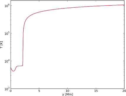
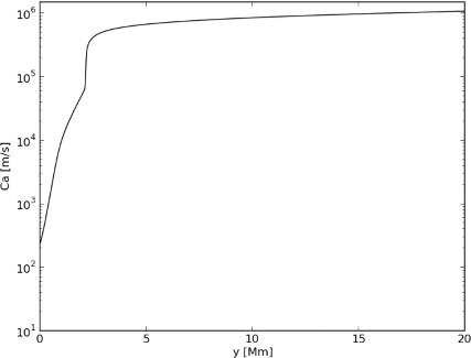
Figure 1: Variation with height $y$ of the equilibrium temperature $T$, given by Avrett & Loeser (2008), (top) and Alfvén speed (bottom).

2.3 Impulsive perturbations

In order to generate Alfvén waves, we perturb the magnetohydrostatic equilibrium by initially (i.e. at $t=0\;$s) launching a localized pulse in the transverse component of ion velocity, $V_{\rm iz}$. The following equation describes this pulse:

$$V_{\rm iz}(y,t=0\;\text{s})=A\;\exp\left(-\frac{(y-y_{\rm 0})^{2}}{w^{2}}\right)\,.$$ (19)

Here, $A$ denotes the amplitude of the pulse, $w$ its width, and $y_{\rm 0}$ its vertical location. By varying $A$ and $y_{\rm 0}$, but holding the width $w$ fixed at $0.2\;$Mm, a similar pulse of different amplitude $A$ is launched in the photosphere or chromosphere.

3 Numerical results

In order to study Alfvén waves in the inhomogeneous and only partially ionized lower layers of the solar atmosphere, we have to rely on numerical simulations. In our model, initially (at $t=0\;$s), an ion velocity pulse described by Eq. (19) is injected into the simulation domain specified as $(-0.08,0.08)\times(-0.5,60)\;$Mm². We use the JOANNA code (Wójcik et al. 2020) to perform the numerical simulations, that is, to solve the two-fluid equations presented and discussed in the previous section. Indeed, this code solves the initial-boundary value problem for the specified two-fluid model. All plasma variables are initialised with their magnetohydrostatic values at the lower and upper boundaries of the simulation domain and held fixed in time throughout the simulation. Setting non-reflecting or absorbing boundary conditions along the gravity action is a formidable and still not fully solved task. We have implied the simplest conceivable boundary conditions with all plasma quantities set to their equilibrium values. Such conditions being supplemented by a well stretched grid along the $y$-direction is found to significantly reduce reflections of the incoming signal. The part of the simulation domain specified by $-0.5\;\text{Mm}\leq y\leq 4.62\;$Mm is divided into 512 grid cells, leading to a numerical grid cell size $\Delta y=10\;$km in that area. The region higher up is covered by 128 grid cells and in this part of the computational domain the grid is stretched, that is, the size of the grid cells steadily grows with height. At the side ($x-$) boundaries, so-called ”open” boundary conditions are implemented, meaning that the $x$-derivatives of all the plasma quantities are set to zero.

3.1 Numerical verification test

Before starting any simulation, we first verify the numerical accuracy by trying to quantify the numerical errors. One test consists of running the code without any initial pulse and relaxing the initial (analytical) equilibrium state numerically, that is, allowing the physical system to evolve in time without any external influence. Although a zero–amplitude pulse cannot lead to the generation of Alfvén waves, as a result of the numerical approximation which is due to the discretization of the equations on a mesh with finite resolution, there is some signal present in the vertical ($y-$) component of the ion velocity and temperature in the system. This signal corresponds to magnetoacoustic waves, which are affected by gravity. We can trace these waves by plotting the $V_{\rm iy}$ component in the $(y,t)$plane (Fig. 2, top) and also plotting the relative perturbed ion temperature,

$$\frac{\delta T_{\rm i}}{T}=\frac{T_{\rm i}-T}{T}\,;$$ (20)

see the bottom plot of Fig. 2. We note that the obtained max ($V_{\rm iy})\approx 0.34\;\text{km}\cdot\text{s}^{-1}$, which takes place in the corona at $y\approx 20\;$Mm, and it is very small compared to the local sound speed $c_{\rm s}\approx 100\;\text{km}\cdot\text{s}^{-1}$ there (not shown). The signal propagates upward at an average velocity of $125\;\text{km}\cdot\text{s}^{-1}$, which corresponds to the average sound speed (the average Alfvén velocity in that area is an order of magnitude higher). Similarly, max ($\delta T_{\rm i}/T)=0.0045$, which is also a very small perturbation and it propagates upward at the same velocity as the $V_{\rm iy}$ perturbation. Hence, we infer that for the chosen numerical grid and discretization scheme, the generated numerical noise in the relaxation phase is rather small and does not affect the numerical results presented below.

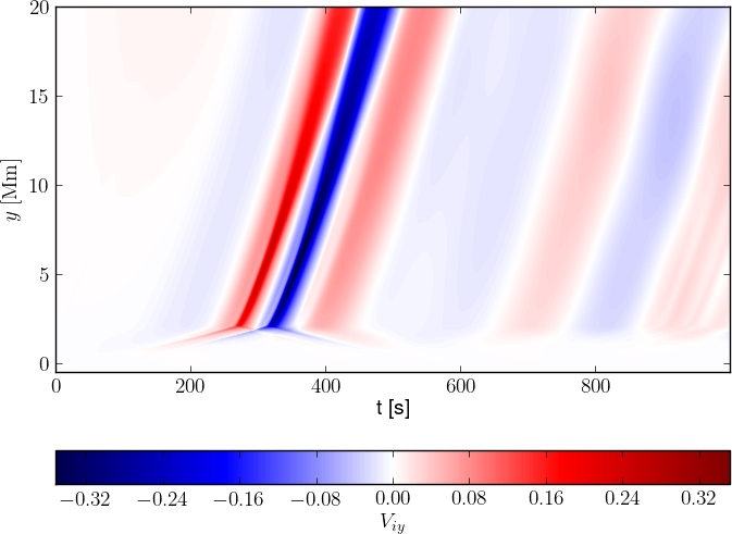
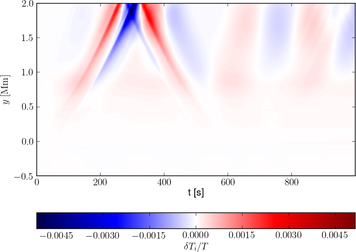
Figure 2: Time–distance plots for $V_{\rm iy}$ (top) and $\delta T_{\rm i}/T$ (bottom) for the initial pulse-free system, i.e., $A=0\;\text{km}\cdot\text{s}^{-1}$. In other words, this plot shows the numerical relaxation of the initial equilibrium state.

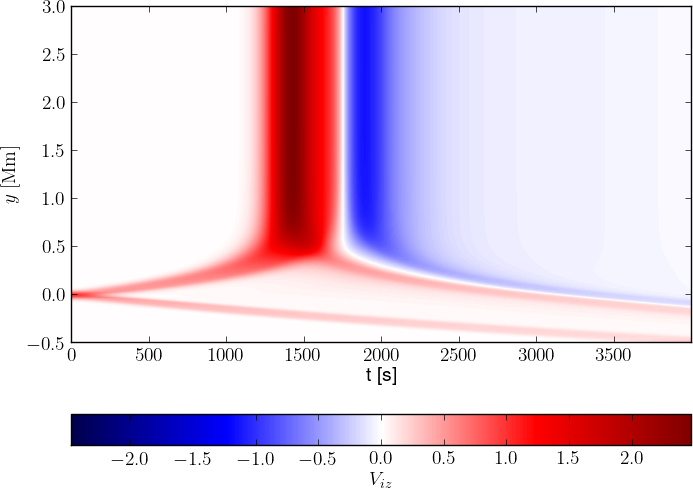
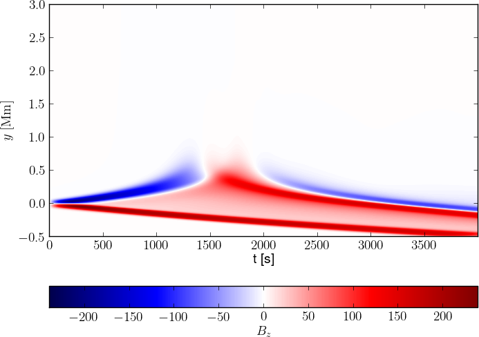
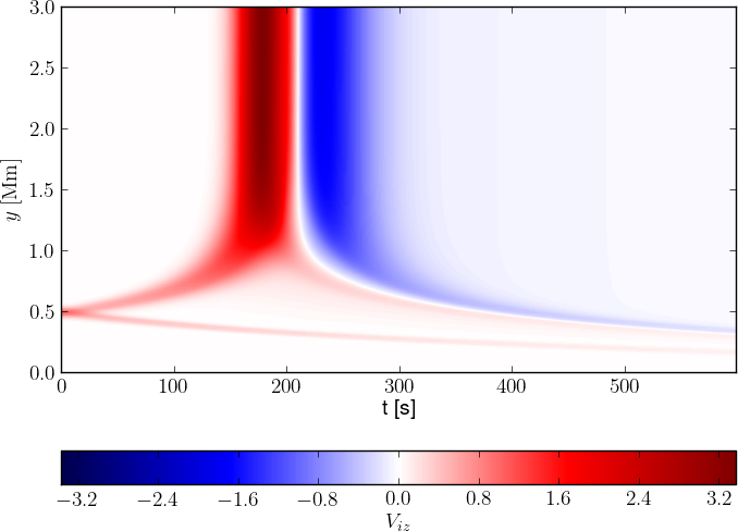
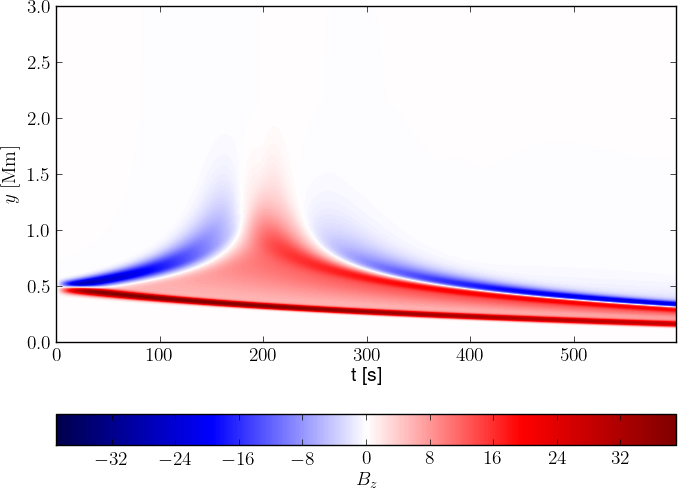
Figure 3: Time–distance plots for $V_{\rm iz}$ (left) and $B_{\rm z}$ (right) for $A=1\;\text{km}\cdot\text{s}^{-1}$, $y_{\rm 0}=0\;$Mm (top) and $y_{\rm 0}=0.5\;$Mm (bottom).

3.2 Small-amplitude Alfvén waves

In this section, we consider small-amplitude Alfvén waves generated by an initial pulse. Figure 3 displays the evolution of the Alfvén waves that are excited by the initial pulse with an amplitude as small as $A=1\;\text{km}\cdot\text{s}^{-1}$ and launched from the bottom of the photosphere, that is, $y_{\rm 0}=0\;$Mm (top plots), and at the top of the photosphere, at $y_{\rm 0}=0.5\;$Mm (bottom plots). The initial pulse splits into two counter-propagating waves, which are damped. This damping results from collisions between ions and neutrals (Leake et al. 2005; Arber et al. 2016; Shelyag et al. 2016; Erdélyi & James 2004; Khodachenko et al. 2004; Forteza et al. 2007; Soler et al. 2019). For the initial pulse at the bottom of the photosphere, the upwardly propagating waves experience partial reflection at $y\approx 0.5\;$Mm (upper plots), corresponding to the top of the photosphere. However, when the initial pulse is located at the top of the photosphere, the reflection takes place at about $y\approx 1.0\;$Mm (bottom plots).

In the case of $y_{\rm 0}=0\;$Mm (Fig. 3, left-top), the reflection takes place after $t\approx 1500\;$s, so the upward propagating waves travel at about $0.33\;\text{km}\cdot\text{s}^{-1}$, which is the average Alfvén velocity in the photosphere (see Fig. 1, bottom). However, for $y_{\rm 0}=0.5\;$Mm (Fig. 3, left-bottom), as a result of higher values of $c_{\rm a}(y)$ in the low chromosphere (Fig. 1, bottom), the waves propagate upward much faster and the reflection therefore occurs much earlier, that is, at about $t\approx 200\;$s, which means that the waves indeed propagate with an average velocity of $2.5\;\text{km}\cdot\text{s}^{-1}$. Some waves propagate higher up, reaching the transition region and the solar corona (left). In the photosphere and the low chromosphere, the amplitudes of the upward- and downward-propagating waves decay with the distance of their propagation. This is a result of ion–neutral collisions taking place in these layers. The left panels of Fig. 3 show that the maximum value of the transversal velocity component is smaller for $y_{\rm 0}=0\;$Mm with max$(V_{\rm iz})\approx 2.5\;\text{km}\cdot\text{s}^{-1}$ than for $y_{\rm 0}=0.5\;$Mm with max$(V_{\rm iz})\approx 3.4\;\text{km}\cdot\text{s}^{-1}$. These maxima are reached in the corona as the plasma density is much lower there.

The right panels of Fig. 3 present plots of a transversal magnetic field $B_{\rm z}$, which is in phase with $V_{\rm iz}$ for the downward-propagating Alfvén waves and in phase opposition for the upward propagating waves. Indeed, here we also observe upward- and downward-propagating waves from the pulse height. The upward-propagating waves experience reflection in both cases (i.e. for $y_{\rm 0}=0\;$Mm and $y_{\rm 0}=0.5\;$Mm) after passing a distance of about $0.5\;$Mm, essentially simultaneously with the reflections seen in the $V_{\rm iz}$ component (Fig. 3, left panels). However, we note that the $B_{\rm z}$ signals evolve differently from the $V_{\rm z}$ perturbations. The $B_{\rm z}$ perturbation amplitude strongly falls off with height and even becomes evanescent above the reflection height, while the $V_{\rm iz}$ component reaches its maximum values there. This difference is well known in the MHD framework, where the evolution of the $B_{\rm z}$ component is described by the following wave equation:

$$\frac{\partial^{2}B_{\rm z}}{\partial t^{2}}-\frac{\partial}{\partial y}\left(c_{a}^{2}\frac{\partial B_{\rm z}}{\partial y}\right)=0\,,$$ (21)

while the transversal component of velocity, $V_{\rm z}$, is governed by the classic wave equation (e.g., Wójcik et al. 2017):

$$\frac{\partial^{2}V_{\rm z}}{\partial t^{2}}-c_{a}^{2}\frac{\partial^{2}V_{\rm z}}{\partial y^{2}}=0\,.$$ (22)

Hence, the increase in the Alfvén velocity $c_{\rm a}$ with height $y$ yields a relatively large damping term ($\sim{\partial B_{\rm z}}/{\partial y}$) in the wave equation for $B_{\rm z}$ which does not appear in the wave equation for $V_{\rm z}$.

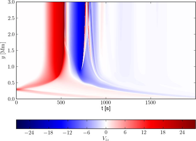
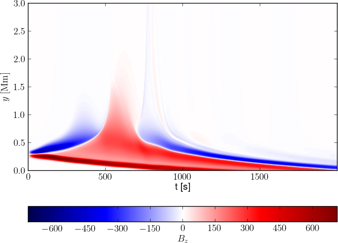
Figure 4: Time–distance plots for: $V_{\rm iz}$ (top-left), $B_{\rm z}$ (top-right), $V_{\rm iz}-V_{\rm nz}$ (bottom-left), and $V_{\rm iy}-V_{\rm ny}$ (bottom-right) in the case of $A=10\;\text{km}\cdot\text{s}^{-1}$ and $y_{\rm 0}=0.3\;$Mm.

3.3 Heating and plasma outflows by large-amplitude Alfvén waves

In this section, we explore the dynamics of large-amplitude Alfvén waves generated by an initial pulse in the lower atmospheric layers of the solar atmosphere. We limit our discussion to the case of an initial pulse of $A=10\;\text{km}\cdot\text{s}^{-1}$. The time–distance profiles of $V_{\rm iz}$ and $B_{\rm z}$ are displayed in Fig. 4 (top), and they globally look similar to those illustrated in Fig. 3 which corresponds to $A=1\;\text{km}\cdot\text{s}^{-1}$. We note that the magnetic field perturbations now travel higher up in the solar atmosphere before being dissipated. The bottom panels of Fig. 4 show the corresponding velocity drifts: $V_{\rm iz}-V_{\rm nz}$ (bottom-left) and $V_{\rm iy}-V_{\rm ny}$ (bottom right). In both bottom panels, it can be seen that the velocity drifts grow with height towards maximum values of $V_{\rm iz}-V_{\rm nz}\approx 1\;\text{km}\cdot\text{s}^{-1}$ and $\max(V_{\rm iy}-V_{\rm ny})\approx 10\;\text{km}\cdot\text{s}^{-1}$, respectively. Due to the fact that the $\max(V_{\rm iy}-V_{\rm ny})$ value is higher than the $\max(V_{\rm iz}-V_{\rm nz})$ value, we infer that magnetoacoustic waves, which are driven by the Alfvén waves, are responsible for the observed heating, which is described by the first term of the right-hand side of Eqs. (11) and (12). The nonlinear coupling of Alfvén waves with magnetoacoustic waves is due to the ponderomotive force. A study of the ponderomotive force in the multi-fluid framework was recently presented by Martínez-Gómez et al. (2018), who investigated impulsively generated Alfvén waves. On the other hand, the fact that the nonlinearly driven magnetoacoustic waves heat the plasma more efficiently has already been discussed; namely by Arber et al. (2016), who used the single-fluid approximation.

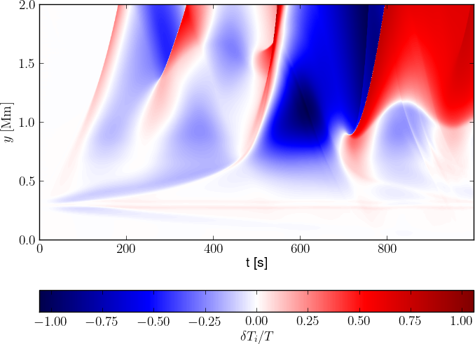
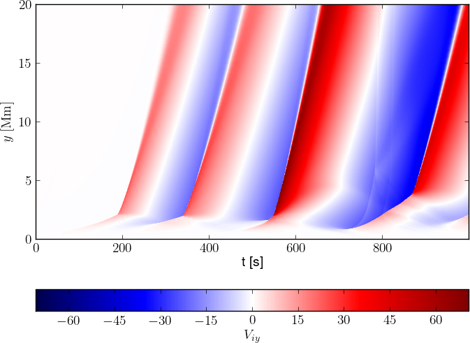
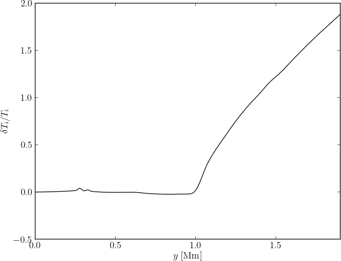
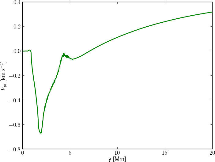
Figure 5: Time-distance plots for $\delta T_{\rm i}/T$ (top-left) and $V_{\rm iy}$ (top-right), perturbed temperature of ions $\delta T_{\rm i}/T$ averaged over time (bottom-left), and the vertical component of ion velocity $V_{\rm iy}$ averaged over time (bottom-right) for $y_{\rm 0}=0.3\;$Mm and $A=10\;\text{km}\cdot\text{s}^{-1}$.

Figure 5 (top panels) presents time–distance plots for the perturbed ion temperature $\delta T_{\rm i}/T$ (left panel) and for the vertical component of the ion velocity $V_{\rm iy}$ (right panel) in the case of $A=10\;\text{km}\cdot\text{s}^{-1}$ and $y_{\rm 0}=0.3\;$Mm (i.e. more or less in the middle of the photosphere). Some correlation between the velocity and temperature signals is discernible from this analysis. Mainly, in the range of $0\;$Mm$\;\leq y\leq 2\;$Mm the signal in $\delta T_{\rm i}/T$ experiences a similar trend to the signal in $V{\rm iy}$ with $\max(V_{\rm iy})\approx 65\;\text{km}\cdot\text{s}^{-1}$ and $\max(\delta T_{\rm i}/T)\approx 1$ taking place for the launching level $y_{\rm 0}=0.3\;$Mm. In the case of the same launching point $y_{0}$, but for a much smaller pulse amplitude, mainly $A=1\;\text{km}\cdot\text{s}^{-1}$, the maximum value of the vertical component of ion velocity is almost 20 times lower than for this amplitude $A=10\;\text{km}\cdot\text{s}^{-1}$ pulse. Similarly, the maximum value of the perturbed relative ion temperature is about 25 times lower for the simulation with amplitude $A=1\;\text{km}\cdot\text{s}^{-1}$. As a matter of fact, for $A=1\;\text{km}\cdot\text{s}^{-1}$ we obtained $\max(V_{\rm iy})\approx 3.6\;\text{km}\cdot\text{s}^{-1}$ and $\max(\delta T_{\rm i}/T)\approx 0.05$ (not shown). The bottom panels of Figure 5 illustrate the perturbed relative ion temperature $\delta T_{\rm i}/T$ averaged over time, and the vertical component of the ion velocity $V_{\rm iy}$ averaged over time. These two quantities are defined as

$$H(y)=\frac{1}{t_{\rm 2}-t_{\rm 1}}\int_{t_{\rm 1}}^{t_{\rm 2}}\frac{\delta T_{\rm i}}{T}\,dt\,,$$ (23)

and

$$V(y)=\frac{1}{t_{\rm 2}-t_{\rm 1}}\int_{t_{\rm 1}}^{t_{\rm 2}}V_{\rm iy}\,dt\,,$$ (24)

where $t_{\rm 1}=0\;$s and $t_{\rm 2}=5000\;$s. We note that the max($H(y)$) takes place for $y=2$ Mm (bottom-left). However, a small increase in temperature is discernible at $y\approx 0.3\;$Mm, the height at which the initial pulse is launched in this case. From the bottom-right panel of Fig. 5, it is inferred that a slow downflow takes place in the lower atmospheric layers up to $y\approx 5\;$Mm. Higher up, on the other hand, there is an upflow or outflow, with a magnitude that is growing with height $y$; it reaches about $0.35\;\text{km}\cdot\text{s}^{-1}$ at $y=20\;$Mm. Below $y\approx 5\;$Mm, the downflow reaches a minimum value of $V_{\rm iy}\approx-0.7\;\text{km}\cdot\text{s}^{-1}$. This means that when going from the lower atmosphere to the corona, the downflow turns into an upflow. A similar scenario was reported by Kayshap et al. (2015) who found even faster downflows of $0-13\;\text{km}\cdot\text{s}^{-1}$ and also faster upflows of $10-12\;\text{km}\cdot\text{s}^{-1}$. Hence, our simple 2.5D numerical findings reveal only the general trend of the vertical flows that is also present in the observational data. This vertical flow can be generated by ponderomotive force originating from Alfvén waves (e.g., Murawski 1992).

Figure 6 displays the relative perturbed ion temperature averaged over height and time. This quantity is defined as (with $H(y)$ given by Eq. (23)):

$$H=\frac{1}{y_{\rm 1}-y_{\rm 0}}\int_{y_{\rm 0}}^{y_{\rm 1}}H(y)\,dy\,,$$ (25)

where $y_{\rm 1}=20\;$Mm. The top panel illustrates $H$ versus the launching height $y_{\rm 0}$. We note that the minimal heating occurs for $y_{\rm 0}=0\;$Mm and the maximal heating $H$ is obtained launching the pulse at $y_{\rm 0}=0.35\;$Mm, which is close to the middle of the photosphere. We also note that $H$ strongly falls off with $y_{\rm 0}>0.35\;$Mm. Such behavior of $H$ versus $y_{\rm 0}$ results from the magnetoacoustic waves that release thermal energy as a result of the ion–neutral collisions and which are driven by Alfvén waves. The ion–neutral collisions are less frequent in the upper layers as the ionization degree is close to one (100%) there.

Figure 6 (bottom panel) illustrates the dependence of the average heating $H$ on the pulse amplitude $A$ for a pulse located at $y_{\rm 0}=0.25\;$Mm. Here, according to our expectations, it is clearly seen that the higher the amplitude of the pulse, the more heat is deposited in the atmosphere.

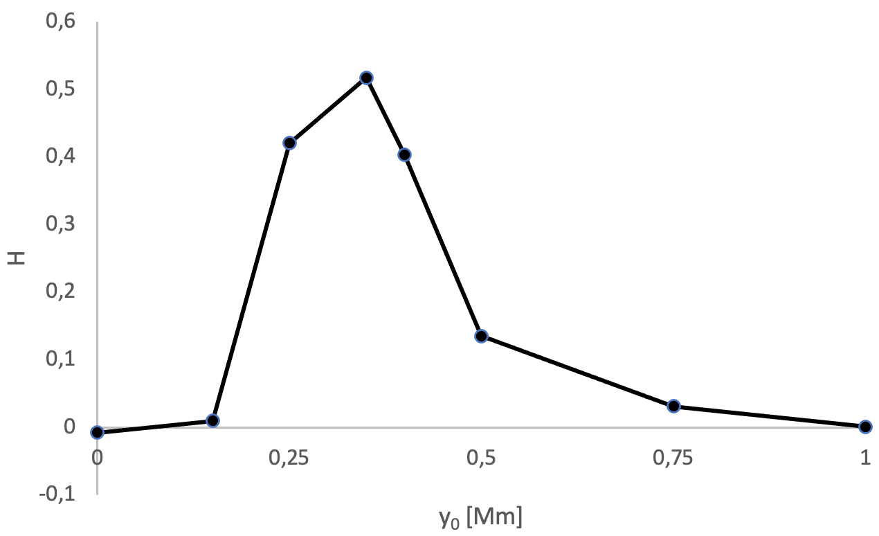
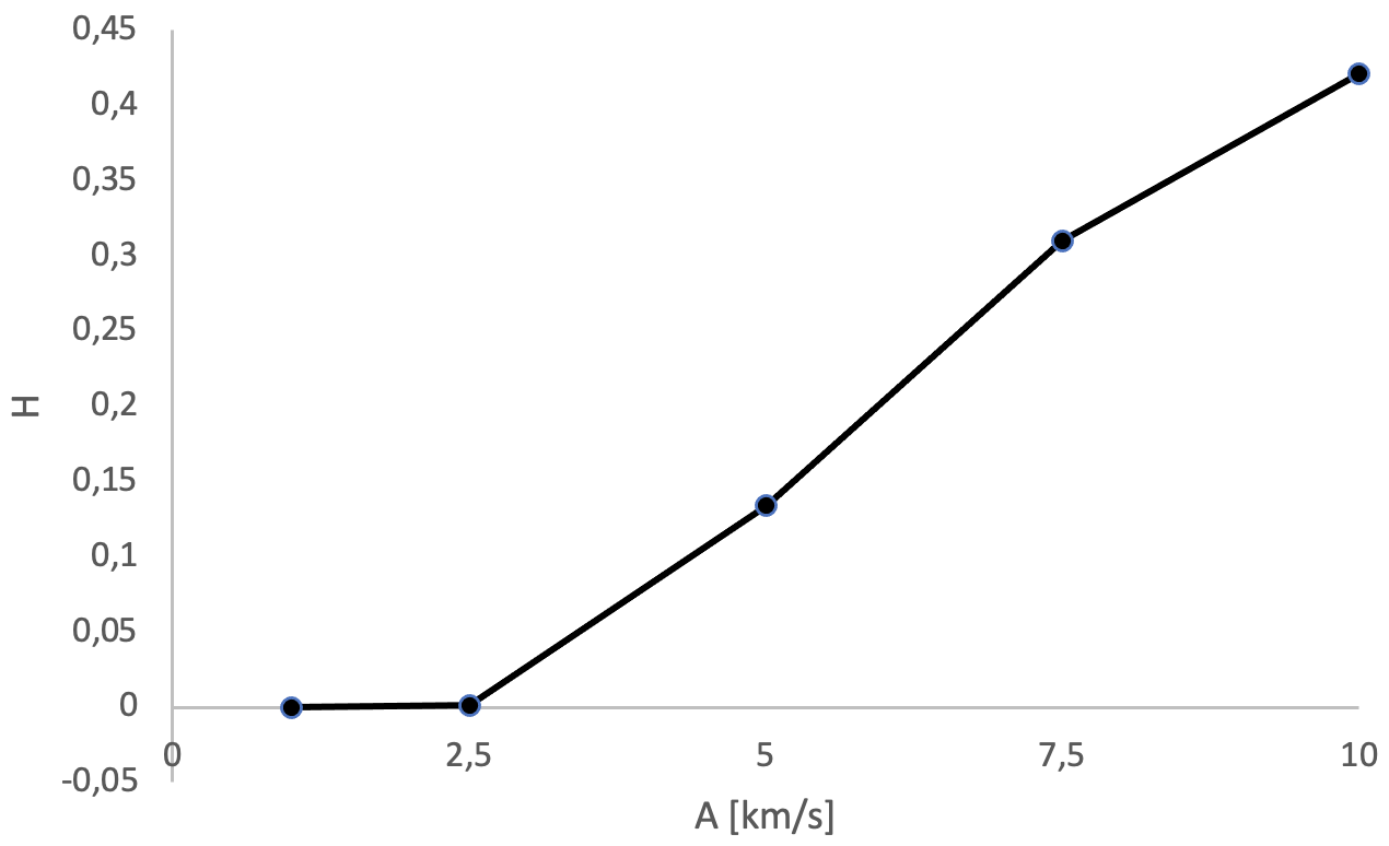
Figure 6: Relative perturbed ion temperature averaged over time and height $H$ vs. pulse launching $y_{\rm 0}$ for $A=10\;\text{km}\cdot\text{s}^{-1}$ (top) and vs. pulse amplitude $A$ for $y_{\rm 0}=0.25\;$Mm (bottom).

4 Summary and Conclusion

In this paper, we present the results of 2.5D simulations of impulsively generated two-fluid Alfvén waves. We show that as a consequence of ion–neutral collisions (e.g., Ballester et al. 2018), large amplitude Alfvén waves generated in the photosphere and chromosphere can contribute to the heating of the chromosphere (e.g., Murawski et al. 2020). These waves can also drive plasma outflows, which higher up can become more substantial and constitute the origin of the solar wind. However, the magnitude of the flows is found to be rather moderate and much lower than the observed in- and outflows by Tian et al. (2009) and Kayshap et al. (2015). Hence, we conclude that impulsively generated two-fluid Alfvén waves with an initial amplitude $A=10\;\text{km}\cdot\text{s}^{-1}$ are not able to explain the observational data, even though the obtained flow amplitudes are in the observed ranges. Nevertheless, the magnitude of the obtained plasma heating is proportional to the pulse amplitude. We find that the maximum heating occurs for the pulse launched from the middle of the photosphere. The maximum of the averaged relative temperature $H$ in the chromosphere increases by about 50%. The pulses launched from the low photosphere and in the chromosphere do not substantially affect the chromosphere temperature (Fig. 6, top). Also, the magnitude of the obtained outflows grows with the amplitude of the pulse. In particular, in the case of the pulse launched from the middle of the photosphere and with an amplitude $A\leq 2.5\;\text{km}\cdot\text{s}^{-1}$, the averaged heating $H$ is negligibly small. For larger values of the amplitude $A$, the trend in $H(A)$ is essentially linear with $H\approx 0.42$ for $A=10\;\text{km}\cdot\text{s}^{-1}$ (Fig. 6, bottom).

Our model is based on the two-fluid equations in which the only source of plasma heating are ion–neutral collisions. Hence, more realistic models that include other nonideal and nonadiabatic effects are required to more accurately describe the solar atmosphere and make the simulations more realistic. Such models are left for future studies and the obtained results will be reported elsewhere.

References

- Alfvén (1942) Alfvén, H. 1942, Nature, 150, 405
- Arber et al. (2016) Arber, T. D., Brady, C. S., & Shelyag, S. 2016, ApJ, 817, 94
- Aschwanden (2005) Aschwanden, M. J. 2005, Physics of the Solar Corona. An Introduction with Problems and Solutions (2nd edition)
- Athay (1976) Athay, R. G. 1976, The solar chromosphere and corona: Quiet sun, Vol. 53
- Avrett (2003) Avrett, E. H. 2003, in Astronomical Society of the Pacific Conference Series, Vol. 286, Current Theoretical Models and Future High Resolution Solar Observations: Preparing for ATST, ed. A. A. Pevtsov & H. Uitenbroek, 419
- Avrett & Loeser (2008) Avrett, E. H. & Loeser, R. 2008, ApJS, 175, 229
- Baker et al. (2021) Baker, D., Stangalini, M., Valori, G., et al. 2021, ApJ, 907, 16
- Ballester et al. (2018) Ballester, J. L., Alexeev, I., Collados, M., et al. 2018, Space Sci. Rev., 214, 58
- Braginskii (1965) Braginskii, S. I. 1965, Reviews of Plasma Physics, 1, 205
- Erdélyi & James (2004) Erdélyi & James. 2004, A&A, 427, 1055
- Forteza et al. (2007) Forteza, P., Oliver, R., Ballester, J. L., & Khodachenko, M. L. 2007, A&A, 461, 731
- Haerendel (1992) Haerendel, G. 1992, Nature, 360, 241
- Hollweg (1978) Hollweg, J. V. 1978, Sol. Phys., 56, 305
- Hollweg (1981) Hollweg, J. V. 1981, Sol. Phys., 70, 25
- Hollweg et al. (1982) Hollweg, J. V., Jackson, S., & Galloway, D. 1982, Sol. Phys., 75, 35
- Jess et al. (2009) Jess, D. B., Mathioudakis, M., Erdélyi, R., et al. 2009, Science, 323, 1582
- Kayshap et al. (2015) Kayshap, P., Banerjee, D., & Srivastava, A. K. 2015, Sol. Phys., 290, 2889
- Khodachenko et al. (2004) Khodachenko, Arber, T. D., Rucker, H. O., & Hanslmeier, A. 2004, A&A, 422, 1073
- Khomenko (2017) Khomenko, E. 2017, Plasma Physics and Controlled Fusion, 59, 014038
- Kudoh & Shibata (1999) Kudoh, T. & Shibata, K. 1999, ApJ, 514, 493
- Kuźma et al. (2017) Kuźma, B., Murawski, K., Kayshap, P., et al. 2017, ApJ, 849, 78
- Leake et al. (2005) Leake, J. E., Arber, T. D., & Khodachenko, M. L. 2005, A&A, 442, 1091
- Marsch et al. (2008) Marsch, E., Tian, H., Sun, J., Curdt, W., & Wiegelmann, T. 2008, ApJ, 685, 1262
- Martínez-Gómez et al. (2018) Martínez-Gómez, D., Soler, R., & Terradas, J. 2018, ApJ, 856, 16
- Matsumoto & Suzuki (2012) Matsumoto, T. & Suzuki, T. K. 2012, ApJ, 749, 8
- McIntosh (2012) McIntosh, S. W. 2012, Space Sci. Rev., 172, 69
- McIntosh et al. (2011) McIntosh, S. W., de Pontieu, B., Carlsson, M., et al. 2011, Nature, 475, 477
- Murawski (1992) Murawski, K. 1992, Sol. Phys., 139, 279
- Murawski et al. (2020) Murawski, K., Musielak, Z. E., & Wójcik, D. 2020, ApJ, 896, L1
- Nakariakov & Verwichte (2005) Nakariakov, V. M. & Verwichte, E. 2005, Living Reviews in Solar Physics, 2, 3
- Ofman (2010) Ofman, L. 2010, Living Reviews in Solar Physics, 7, 4
- Okamoto & De Pontieu (2011) Okamoto, T. J. & De Pontieu, B. 2011, ApJ, 736, L24
- Osterbrock (1961) Osterbrock, D. E. 1961, ApJ, 134, 347
- Piddington (1956) Piddington, J. H. 1956, The Observatory, 76, 21
- Roy & Pandey (2002) Roy, S. & Pandey, B. P. 2002, Physics of Plasmas, 9, 4052
- Shelyag et al. (2016) Shelyag, S., Khomenko, E., de Vicente, A., & Przybylski, D. 2016, ApJ, 819, L11
- Shestov et al. (2017) Shestov, S. V., Nakariakov, V. M., Ulyanov, A. S., Reva, A. A., & Kuzin, S. V. 2017, ApJ, 840, 64
- Soler et al. (2017) Soler, R., Terradas, J., Oliver, R., & Ballester, J. L. 2017, ApJ, 840, 20
- Soler et al. (2019) Soler, R., Terradas, J., Oliver, R., & Ballester, J. L. 2019, ApJ, 871, 3
- Song & Vasyliūnas (2011) Song, P. & Vasyliūnas, V. M. 2011, Journal of Geophysical Research (Space Physics), 116, A09104
- Srivastava et al. (2017) Srivastava, A. K., Shetye, J., Murawski, K., et al. 2017, Scientific Reports, 7, 43147
- Tian et al. (2009) Tian, H., Marsch, E., Curdt, W., & He, J. 2009, ApJ, 704, 883
- Tu et al. (2005) Tu, C.-Y., Zhou, C., Marsch, E., et al. 2005, Science, 308, 519
- Uchida & Kaburaki (1974) Uchida, Y. & Kaburaki, O. 1974, Sol. Phys., 35, 451
- Vranjes & Krstic (2013) Vranjes, J. & Krstic, P. S. 2013, A&A, 554, A22
- Wójcik et al. (2020) Wójcik, D., Kuźma, B., Murawski, K., & Musielak, Z. E. 2020, A&A, 635, A28
- Wójcik et al. (2019) Wójcik, D., Kuźma, B., Murawski, K., & Srivastava, A. K. 2019, ApJ, 884, 127
- Wójcik et al. (2017) Wójcik, D., Murawski, K., Musielak, Z. E., Konkol, P., & Mignone, A. 2017, Sol. Phys., 292, 31
- Yang & Xiang (2016) Yang, S. & Xiang, Y. 2016, ApJ, 819, L24
- Zaqarashvili et al. (2011) Zaqarashvili, T. V., Khodachenko, M. L., & Rucker, H. O. 2011, A&A, 529, A82
- Zaqarashvili et al. (2013) Zaqarashvili, T. V., Khodachenko, M. L., & Soler, R. 2013, A&A, 549, A113