A scaling relationship for non-thermal radio emission from ordered magnetospheres: from the top of the Main Sequence to planets

Abstract

In this paper, we present the analysis of incoherent non-thermal radio emission from a sample of hot magnetic stars, ranging from early-B to early-A spectral type. Spanning a wide range of stellar parameters and wind properties, these stars display a commonality in their radio emission which presents new challenges to the wind scenario as originally conceived. It was thought that relativistic electrons, responsible for the radio emission, originate in current sheets formed where the wind opens the magnetic field lines. However, the true mass-loss rates from the cooler stars are too small to explain the observed non-thermal broadband radio spectra. Instead, we suggest the existence of a radiation belt located inside the inner-magnetosphere, similar to that of Jupiter. Such a structure explains the overall indifference of the broadband radio emissions on wind mass-loss rates. Further, correlating the radio luminosities from a larger sample of magnetic stars with their stellar parameters, the combined roles of rotation and magnetic properties have been empirically determined. Finally, our sample of early-type magnetic stars suggests a scaling relationship between the non-thermal radio luminosity and the electric voltage induced by the magnetosphere’s co-rotation, which appears to hold for a broader range of stellar types with dipole-dominated magnetospheres (like the cases of the planet Jupiter and the ultra-cool dwarf stars and brown dwarfs). We conclude that well-ordered and stable rotating magnetospheres share a common physical mechanism for supporting the generation of non-thermal electrons.

1 Introduction

The magnetic fields of magnetic main-sequence B/A type stars have, on average, a strength of a few kG (Sikora et al., 2019b; Shultz et al., 2019c) with stable field topologies (Shultz et al., 2018). The magnetic field topology of the majority of them can be described in terms of the oblique rotator model (ORM), predominantly involving a centered dipole field that is tilted to the stellar rotation axis (Babcock, 1949; Stibbs, 1950). The presence of a large-scale magnetic field induces surface chemical anisotropies on the stellar surface, making these stars variable as a consequence of stellar rotation (Krtička et al., 2007). In general early-type magnetic stars are recognized based on their chemical peculiarities, and are classified as Ap/Bp stars (Preston, 1974).

The MiMeS (Magnetism in Massive Stars; Wade et al., 2016) and BOB (B fields in OB stars; Morel et al., 2015) spectropolarimetric surveys concluded that magnetism characterizes about $6$–8% of the stars across the upper main-sequence (MS) (Fossati et al., 2015; Wade et al., 2016; Grunhut et al., 2017; Sikora et al., 2019a), with the incidence rate almost constant for stars ranging from the O to the Ap stars. The magnetism almost certainly has a fossil origin (Braithwaite & Spruit, 2004; Duez & Mathis, 2010; Neiner et al., 2015) rather than being created by a magnetic dynamo as in late-type stars; this is supported by the magnetic field decay during the stellar life (Landstreet et al., 2007, 2008; Fossati et al., 2016; Sikora et al., 2019b; Petit et al., 2019; Shultz et al., 2019c). Further, stellar mergers have been proposed as origin of the strong magnetic fields observed at the top of the MS (Bogomazov & Tutukov, 2009; Schneider et al., 2016, 2019; Keszthelyi et al., 2021).

The early-type magnetic stars are sufficiently hot to radiatively drive stellar wind, which in the presence of their large-scale magnetic fields may be strongly aspherical (Babel & Montmerle, 1997; Ud-Doula & Owocki, 2002). The wind plasma accumulates at low magnetic latitudes (inner magnetosphere), whereas it freely propagates along directions aligned with the magnetic poles (Shore, 1987; Shore & Brown, 1990; Leone, 1993).

This concept has led to the magnetically confined wind shock (MCWS) model (Babel & Montmerle, 1997). In the presence of large-scale magnetic fields, the wind cannot freely propagate spherically, and the ionized wind flow is channeled by the magnetic field lines. At the magnetic equator, wind streams arising from the opposite magnetic hemispheres collide and shock, producing X-rays (Oskinova et al., 2011; Nazé et al., 2014; Robrade, 2016). Detailed modeling of the magnetospheres of hot magnetic stars has progressively developed (Ud-Doula & Owocki, 2002; Ud-Doula, Townsend & Owocki, 2006, 2008, 2013, 2014; Owocki et al., 2016; Daley-Yates et al., 2019; Munoz et al., 2020).

Rapidly rotating magnetic stars require the presence of strong magnetic fields to enable formation of centrifugal magnetospheres (Maheswaran & Cassinelli, 2009; Petit et al., 2013; Shultz et al., 2019c), where the centrifugal force is strong enough to balance the gravitational infall of the circumstellar ionized material. The magnetospheric ionized matter is forced to rigidly co-rotate with the stars, producing a rigidly rotating magnetosphere (RRM), which is characterized by typical signatures recognized in the H$\alpha$ line profile and photometric variability (Townsend & Owocki, 2005; Townsend, 2008).

Table 1: Stars of the sample and corresponding stellar parameters.

				$D$	$T_{\mathrm{eff}}$	$R_{\ast}$	$P_{\mathrm{rot}}^{{\dagger}}$	$B_{\mathrm{p}}$	Frac. MS age	$L_{\nu,\mathrm{rad}}$
ID	HD	Alt. name	Sp. type	(pc)	(kK)	(R⊙)	(d)	(kG)		(erg s-1 Hz-1)
1	12447	$\alpha$ Psc A	A2 SiSrCr	$~{}~{}50(2)$	$10.2(0.5)$	$2.6(0.2)^{(3)}$	1.4907(8)(17)	$1.19\pm 0.2^{(33)}$	$0.58(0.2)^{(36)}$	$1.8(0.6)\times 10^{15}$
2	19832	56 Ari	B8 Si	$~{}~{}124(3)~{}~{}$	$12.5(0.5)$	$2.3(0.3)^{(4)}$	0.72795(1)(18)	$2.7^{+0.6}_{-0.3}$(4)	$0.51(0.26)^{(36)}$	$~{}~{}~{}~{}~{}~{}9(2)\times 10^{15}$
3	27309	56 Tau	A0 SiCr	$~{}~{}90(2)$	$12.0(0.5)$	${2.3(0.3)^{(10)}}$	1.56882(5)(18)	$3.6^{+1.98}_{-0.58}$(10)	$0.41(0.33)^{(10)}$	$3.6(0.6)\times 10^{15}$
4	34452	IQ Aur	B9 Si	$~{}~{}145(4)~{}~{}$	$14.1(0.5)$	$3.1(0.3)^{(5)}$	2.466264(5)(19)	$\approx 4^{(34)}$	$0.40^{+0.15}_{-0.21}$(37)	$1.0(0.3)\times 10^{16}$
5	35298	V1156 Ori	B6 He-wk	$~{}~{}371(9)~{}~{}$	$15.8(0.8)$	$2.42(0.09)^{(6)}$	1.85458(3)(20)	$11.2\pm 1^{(6)}$	$0.06(0.02)^{(6)}$	$~{}~{}~{}~{}~{}~{}4(2)\times 10^{16}$
6	35502	BD-02 1241	B5V He-wk	$383(9)$	$18.4(0.6)$	$3.0(0.1)^{(6)}$	0.853807(3)(7)	$7.3\pm 0.5^{(6)}$	$0.11(0.03)^{(6)}$	$~{}~{}~{}~{}~{}~{}4(1)\times 10^{17}$
7	36485∗	$\delta$ Ori C	B3Vp He-s	$~{}~{}390(10)$	$20.0(2.0)$	$2.97(0.08)^{(6)}$	1.47775(4)(21)	$8.9\pm 0.2^{(6)}$	$0.05(0.02)^{(6)}$	$1.7(0.6)\times 10^{17}$
8	37017∗	V1046 Ori	B2 He-s	$420(35)^{b}$	$21.0(2.0)$	$3.6(0.2)^{(6)}$	0.901186(2)(20)	$6.2\pm 0.9^{(6)}$	$0.13(0.03)^{(6)}$	$~{}~{}~{}~{}~{}~{}4(2)\times 10^{17}$
9	37479∗	$\sigma$ Ori E	B2 Vp He-s	$440(20)$	$23.0(2.0)$	$3.39^{+0.06}_{-0.04}$(6)	1.190833(3)(22)	$10.5\pm 1.5^{(4)}$	$0.06^{+0.02}_{-0.03}$(6)	$~{}~{}~{}~{}~{}~{}7(3)\times 10^{17}$
10	40312	$\theta$ Aur	A0 Si	$~{}~{}58(1)$	$10.2(0.4)$	$4.6(0.2)^{(8)}$	3.61866(1)(23)	$0.69\pm 0.01^{(8)}$	$1.00^{+0.01}_{-0.06}$(10)	$1.2(0.6)\times 10^{15}$
11	79158	36 Lyn	B9 He-wk	$175(6)$	$13.1(0.7)$	$3.4(0.7)^{(9)}$	3.83476(4)(24)	$3.57\pm 0.36^{(9)}$	$0.84^{+0.08}_{-0.1}$(37)	$1.6(0.8)\times 10^{16}$
12	112413	$\alpha^{2}$ CVn	A0 EuSiCr	$~{}~{}35(1)$	$11.5(0.5)$	$2.5(0.3)^{(10)}$	5.46913(8)(16)	$3.46^{+2.29}_{-0.69}$(16)	$0.53^{+0.28}_{-0.31}$(10)	$1.1(0.7)\times 10^{15}$
13	118022	78 Vir††	A2 CrEuSr	$~{}58.3(0.8)$	$~{}~{}9.4(0.5)$	$2.0(0.1)^{(10)}$	3.722084(2)(25)	$3.65^{+0.61}_{-0.37}$(16)	$0.39^{+0.32}_{-0.25}$(10)	$~{}~{}~{}~{}~{}~{}2(1)\times 10^{15}$
14	124224∗	CU Vir	B9 Si	$~{}~{}72(1)$	$12.2(0.5)$	$2.1(0.1)^{(11)}$	0.520714(1)(26)	$3.8\pm 0.2^{(11)}$	$0.13^{+0.42}_{-0.09}$(10)	$1.8(0.6)\times 10^{16}$
15	133652	HZ Lup	B9 Si	$121(1)$	$12.8(0.5)$	$2.2(0.2)^{(12)}$	2.30405(2)(12)	$6.1\pm 0.7^{(12)}$	$0.06(0.02)^{(38)}$	$~{}~{}~{}~{}~{}~{}4(2)\times 10^{15}$
16	133880∗	HR 5624	B9 Si	$104(3)$	$12.0(0.5)$	$2.0(0.3)^{(13)}$	0.877476(9)(13)	$9.6\pm 1^{(13)}$	$0.05(0.02)^{(38)}$	$3.5(1.5)\times 10^{16}$
17	142184∗	HR 5907	B2V He-s	$141(3)$	$18.5(0.5)$	$2.8(0.1)^{(6)}$	0.508276(15)(27)	$9\pm 2^{(6)}$	$0.05_{-0.05}^{+0.1}$(6)	$~{}~{}~{}~{}~{}~{}2(1)\times 10^{18}$
18	142301∗	3 Sco	B8 He-wk Si	$148(3)$	$16.2(0.7)$	$2.42(0.02)^{(4)}$	1.45957(5)(28)	$12.5^{+9}_{-0.3}$(4)	$0.04(0.01)^{(38)}$	$~{}~{}~{}~{}~{}~{}9(2)\times 10^{16}$
19	142990	V913 Sco	B7 He-wk	$146(4)$	$17.0(0.7)$	$2.79(0.06)^{(6)}$	0.978891793(6)(29)	$4.7\pm 0.4^{(6)}$	$0.06(0.01)^{(6)}$	$4.7(0.8)\times 10^{16}$
20	144334	HR 5988	B8 He-wk	$133(2)$	$15.2(0.7)$	$2.27(0.04)^{(4)}$	1.49499(4)(4)	$3.6\pm 0.3^{(4)}$	$0.04(0.01)^{(38)}$	$~{}~{}~{}~{}~{}~{}7(3)\times 10^{15}$
21	145501	$\nu$ Sco C	B9 Si	$141(1)$	$14.0(0.5)$	$2.26(0.06)^{(4)}$	1.02648(1)(4)	$5.8\pm 0.3^{(4)}$	$0.04(0.02)^{(38)}$	$3.8(0.7)\times 10^{15}$
22	147932∗	$\rho$ Oph C	B5Va	$134(1)$	$17.0(1.0)^{(1)}$	$3.3(0.2)^{(14)}$	0.8639(1)(30)	$13.2_{-1.2}^{+2.6}$(14)	$0.12_{-0.03}^{+0.04}$(39)	$~{}~{}~{}~{}~{}~{}4(1)\times 10^{17}$
23	147933∗	$\rho$ Oph A	B2Va	$140(4)$	$20.8(0.5)^{(2)}$	$4.5(0.6)^{(15)}$	0.747326(2)(2)	$2.7_{-0.7}^{+0.9}$(2)	$0.26(0.06)^{(39)}$	$1.7(0.5)\times 10^{17}$
24	170000	$\phi$ Dra	A0 Si	$~{}~{}~{}~{}93(3)^{c}$	$11.4(0.4)$	$3.7(0.1)^{(10)}$	1.71665(9)(18)	$1.75^{+0.14}_{-0.16}$(16)	$0.88^{+0.09}_{-0.03}$(10)	$~{}~{}~{}~{}~{}~{}6(2)\times 10^{15}$
25	175362	HR 7129	B6 He-wk	$153(4)$	$16.9(0.7)$	$2.7(0.2)^{(6)}$	3.67381(1)(20)	$17.0^{+0.6}_{-0.4}$(6)	$0.06_{-0.06}^{+0.11}$(6)	$~{}~{}~{}~{}~{}~{}9(3)\times 10^{15}$
26	176582	V545 Lyr	B5 He-wk	$301(4)$	$17.2(0.7)$	$3.21(0.06)^{(6)}$	1.58221(5)(18)	$5.4\pm 0.2^{(6)}$	$0.32(0.06)^{(6)}$	$~{}~{}~{}~{}~{}~{}4(1)\times 10^{16}$
27	182180∗	HR 7355	B2Vn	$233(6)$	$19.8(1.4)$	$3.2(0.1)^{(6)}$	0.5214404(6)(31)	$9.5\pm 0.6^{(6)}$	$0.09(0.09)^{(6)}$	$~{}~{}~{}~{}~{}~{}9(3)\times 10^{17}$
28	215441	GL Lac†††	B9 Si	$~{}~{}490(10)$	$14.7(0.5)$	${3(1)}^{(40)}$	9.487574(3)(32)	$\approx 62.4^{(35)}$	$0.2(0.2)^{(40)}$	$~{}~{}~{}~{}~{}~{}3(1)\times 10^{17}$

• ^∗ Radio spectrum available. ^† The uncertainties in the least significant digit of the rotation are given in parentheses. ^†† First magnetic star (Babcock, 1947), except the Sun. ^††† Babcock’s star (mean field $\approx 34$ kG; Babcock, 1960). ^a Spectral type from Simbad. ^b HD 37017 assumed at the average distance of the stars belonging to the Ori OB1c cluster (Landstreet et al., 2007), see discussion reported in Shultz et al. (2019a). ^c Distance from Hipparcos (van Leeuwen, 2007).

• ⁽¹⁾Alecian et al., 2014; ⁽²⁾Leto et al., 2020a; ⁽³⁾Allende Prieto & Lambert, 1999; ⁽⁴⁾Shultz et al., 2020; ⁽⁵⁾Pasinetti Fracassini et al., 2001; ⁽⁶⁾Shultz et al., 2019c; ⁽⁷⁾Sikora et al., 2016; ⁽⁸⁾Kochukhov, Shultz & Neiner, 2019; ⁽⁹⁾Wade et al., 2006; ⁽¹⁰⁾Sikora et al., 2019a; ⁽¹¹⁾Kochukhov et al., 2014; ⁽¹²⁾Bailey & Landstreet, 2015; ⁽¹³⁾Bailey et al., 2012; ⁽¹⁴⁾Leto et al., 2020b; ⁽¹⁵⁾Pillitteri et al., 2018; ⁽¹⁶⁾Sikora et al., 2019b; ⁽¹⁷⁾Borra & Landstreet, 1980; ⁽¹⁸⁾Bernhard, Hümmerich & Paunzen, 2020; ⁽¹⁹⁾Bohlender, Landstreet & Thompson, 1993; ⁽²⁰⁾Shultz et al., 2018; ⁽²¹⁾Leone et al., 2010; ⁽²²⁾Townsend et al., 2010; ⁽²³⁾Krtička et al., 2015; ⁽²⁴⁾Oksala et al., 2018; ⁽²⁵⁾Catalano & Leone, 1994; ⁽²⁶⁾Pyper et al., 2013; ⁽²⁷⁾Grunhut et al., 2012; ⁽²⁸⁾Shore et al., 2004; ⁽²⁹⁾Shultz et al., 2019b; ⁽³⁰⁾Rebull et al., 2018; ⁽³¹⁾Rivinius et al., 2013; ⁽³²⁾North & Adelman, 1995; ⁽³³⁾Glagolevskij & Gerth, 2010; ⁽³⁴⁾Babel & Montmerle, 1997; ⁽³⁵⁾Landstreet & Mathys, 2000; ⁽³⁶⁾Wraight et al., 2012; ⁽³⁷⁾Kochukhov & Bagnulo, 2006; ⁽³⁸⁾Landstreet et al., 2007; ⁽³⁹⁾ Schneider et al., 2014; ⁽⁴⁰⁾ Wade, 1997.

Significant non-thermal radio emission is dependent on the presence of a strong magnetic field in the plasma environment of early-type magnetic stars. Indeed, about 25% of the magnetic B/A type stars are non-thermal radio sources (Drake et al., 1987; Linsky, Drake & Bastian, 1992; Leone, Trigilio & Umana, 1994). The prevailing scenario to explain their radio emission is related to the interaction between the radiatively driven ionized stellar wind and the ambient magnetic field (André et al., 1988). The ionized stellar wind opens the magnetic field lines, and a continuous acceleration occurs in the current sheets in the equatorial plane. The distance at which the radiative wind kinetic energy density equals the magnetic energy density is the Alfvén radius ($R_{\mathrm{A}}$). Non-thermal plasma particles, propagating within the stellar magnetosphere, radiate in the radio regime through the incoherent gyro-synchrotron mechanism and produce continuum radio emission that is partially circularly polarized.

The main observational features of non-thermal radio emission from early-type magnetic stars are nearly flat spectra, and rotational modulation, both for the total intensity (Stokes $I$) and circular polarization (Stokes $V$). The polarization level for incoherent non-thermal radio emission increases with frequency, reaching levels of $\approx 10$–20% (Leto et al., 2012, 2018, 2019, 2020a). Multifrequency radio light curves for Stokes $I$ and $V$ have been successfully reproduced using a synthetic 3D model of gyro-synchrotron emission from an oblique dipole field and co-rotating magnetosphere (Trigilio et al., 2004; Leto et al., 2006).

Superimposed on the incoherent radio emission, highly polarized (up to $100$%) strong pulses of coherent emission have also been detected at low frequencies in seven early-type magnetic stars (Trigilio et al., 2000; Das, Chandra & Wade, 2018; Das et al., 2019a, b; Leto et al., 2019, 2020a, 2020b). This amplified pulsed emission is stimulated via the coherent Electron Cyclotron Maser (ECM) emission mechanism (Wu & Lee, 1979; Melrose & Dulk, 1982). ECM is also the process explaining highly beamed auroral radio emissions (AREs) from the magnetized planets of the solar system (Zarka, 1998). In Jupiter, auroral X-rays (Branduardi-Raymont et al., 2007, 2008) arise from the footprints of the magnetic field lines where the coherent auroral radio emission originates, at a few stellar radii above the magnetic poles. ARE from some early-type magnetic stars also has corresponding X-ray emission (Pillitteri et al., 2016, 2017; Robrade et al., 2018).

Interestingly, in the lower main sequence, signatures of coherent AREs have also been identified in ultra-cool dwarf stars and brown dwarfs (UCDs) (Berger, 2002; Kao et al., 2018). These cold stars are fully convective, yet a well-ordered dipole-dominated magnetic field topology has been recognized in many of them (Donati et al., 2006; Morin et al., 2010). The magnetic fields of these stars are generated by a rotational-convective dynamo analogous to the Earth’s geodynamo (Christensen, Holzwarth & Reiners, 2009). It is worth noting that in some cases rotationally modulated incoherent non-thermal emission has also been detected (McLean et al., 2011; Williams et al., 2015a).

The aim of this paper is to test the scenario capable of explaining the radio emission of hot magnetic stars, that works for early B-type magnetic stars, through to magnetic stars at the low-temperature boundary of this group (late B/early A). For this purpose, we have identified a sample of B/A type magnetic stars that have been detected at radio wavelengths, and have collected reliable information about their stellar parameters. The stellar sample is described in Section 2. Details regarding the radio measurements of the individual stars are reported in Appendix A. For some stars we collected enough multifrequency radio measurements to produce reliable radio spectra. Model calculations of the radio spectra of this representative sub-sample are discussed in Section 3. The results of the modeling raised a critical issue regarding the assumed wind paradigm that, up to now, has been assumed as a primary engine to support and explain all the observed radio phenomena from early-type magnetic stars (we discuss this in Section 4). We have searched for a possible dependence of the radio luminosity with stellar age in Section 5. By correlating the radio luminosities of the whole sample of stars with the parameters of their stellar magnetospheres, we obtained an empirical relation between the incoherent non-thermal radio luminosity of the B/A magnetic stars and the combined effect of rotation and magnetic properties of their large-scale dipole-dominated magnetospheres, which we describe in Section 6. In Section 7, this new result is applied in a broader context involving other classes of stars (and planets) that radiate incoherent non-thermal radio emission and have large scale dipole dominated magnetospheres, such as Jupiter and the UCDs. In Sec. 8, the scaling relationship for the incoherent non-thermal radio emission has been applied to a small sample of magnetic hot Jupiters to estimate the expected flux levels and the possible detectability. In Section 9 we discuss the possible physical consequences of our results, and in Section 10 we present our conclusions.

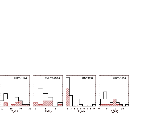
Figure 1: Parameter distributions of the analyzed sample. The sub-sample analyzed in Sec. 3 is shown by the colored areas. Note that the Babcock’s star lies outside the range of the $B_{\mathrm{p}}$ plot at 62.4 kG.

2 The sample

Our sample consists of stars that satisfy two conditions: each star has at least one observation in which radio emission was clearly detected, and stellar and magnetospheric parameters are available for each. The selected sources and stellar parameters with the corresponding references, are listed in Table 1. Each source is identified by the number listed in column 1. Common and alternative names are given in columns 2 and 3. Column 4 lists the spectral types and chemical peculiarities of the selected stars, which together with the effective temperature (column 6), are mainly taken from Netopil et al. (2017) and Shultz et al. (2019a). Column 5 reports the distances of the sources from Gaia Collaboration (2018); in cases when Gaia measurements are not available, references for adopted distances are identified. Radii, rotation periods, and polar magnetic field strengths are given in columns 7, 8 and 9. Column 10 lists the fractional MS ages retrieved from the literature. In two cases the stellar evolutionary state had not previously analyzed, so for these 2 stars (HD 147932 and HD 147933) we used BONNSAI (Schneider et al., 2014) to estimate ages using the evolutionary models given by Brott et al. (2011). Column 11 lists the average radio luminosities of each star obtained from averaging all available radio measurements.

Radio measurements of individual stars have been collected from both published measurements and unpublished observations, acquired by us or retrieved from the VLA data archive. The archival data have been analyzed using the standard reduction steps enabled within the software package casa. We also included data from the New VLA Sky Survey (VLASS) (Lacy et al., 2020). The VLASS observed the sky at $\delta>-40^{\circ}$ and at $\nu=3$ GHz (2 GHz bandwidth). The fluxes have been corrected for systematic errors as reported by Lacy et al. (2019). For the newly obtained radio measurements, we determined fluxes using a gaussian fit to the radio sources (using the standard procedure in casa) located at the sky position of the stars in our sample. Details regarding the radio measurements for individual stars are provided in Appendix A, where the mean (or unique) radio frequencies of all the available flux measurements are also given. Representative frequencies where the stellar radio luminosities have been estimated lie in the range $\approx 3$–13 GHz.

The stellar parameters of our sample ($T_{\mathrm{eff}}$, $R_{\ast}$, $P_{\mathrm{rot}}$, $B_{\mathrm{p}}$) and the corresponding distributions are shown in Fig. 1, where the distributions of the sub-sample analyzed in detail in Sec. 3 are also superimposed. The effective temperatures of the selected stars ranges from $\approx 10$ kK up to near $\approx 25$ kK, with a broad distribution roughly peaked close to $T_{\mathrm{eff}}\approx 15$ kK. The radii of the selected stars cover the range 2–5 R_⊙. The stellar rotation periods of the sample are mainly between $\approx 0.5$ and $\approx 2.5$ days, with a secondary group close to $P_{\mathrm{rot}}\approx 3.5$–4 d. Only two targets have longer rotation periods (third panel of Fig. 1). Finally, the last panel of Fig. 1 shows the polar magnetic field strength distribution. The stars analyzed here have polar magnetic field strengths peaked close to $B_{\mathrm{p}}\approx 3$–4 kG, with a clear secondary peak centered at $B_{\mathrm{p}}\approx 9$–10 kG. Note that Babcock’s star ($B_{\mathrm{p}}=62.4$ kG) is not shown in the fourth panel of Fig. 1 to avoid enlarging the x-axis scale for just this one source.

Figure 2: Radio spectra of the ten stars having enough radio measurements to produce reliable average radio spectra. The data are provided in the tables reported in Appendix A, where details on the individual stars are also described. Open symbols refer to observing frequencies having few measurements (less than three); in these cases the sampling of the stellar rotation period is poor. The modeled radio spectra are superimposed on the observed data. The dotted line show the model extrapolation to higher frequencies.

3 Modeling of a representative sub-sample

Incoherent gyro-synchrotron emission from the magnetospheres of magnetic B/A stars is rotationally modulated as a consequence of the variable projected source area. To conduct a comprehensive study of radio variability ideally multi-frequency radio observations that sample the entire rotation period are needed. A detailed study of the temporal evolution of the broadband radio spectra has been performed only for a few stars, and limited only to narrow ranges of rotational phases (Leto et al., 2012, 2017a, 2018, 2020a).

We collected all available radio measurements for the stars in our sample (Sec. 2). Unfortunately there are many cases in which the data have inadequate coverage of stellar rotational phase, or only a few radio frequencies available. Even so, a representative number of stars ($\approx 35\%$ of the total) do have a large number of multi-frequency radio measurements; their parameter distributions are also highlighted by the colored areas in Fig. 1. Such sub-sample of stars with superior frequency coverage (typically, repeated measurements of at least 5 radio frequencies) are listed in Table 2. Ten stars span nearly the whole range of considered stellar parameters, except for the rotation period. All the stars of this sub-sample have short periods (less than 1.5 d). This is an expected bias because only a few observing facilities are able to detect stellar radio emission, and the ability to perform radio measurements covering large portions of the stellar rotation is naturally biased toward short-period cases. For this sub-sample of ten stars, we obtained reliable radio spectra from averaging observations repeated over more than 3 epochs acquired at the same frequency. The average spectra of these stars are shown in Fig. 2.

3.1 Model description

The 3D model of stellar radio emission from a dipole dominated magnetosphere (Trigilio et al., 2004; Leto et al., 2006) has been previously used to successfully reproduce the multi-wavelength radio light curves of early-type magnetic stars, both for the total intensity (Stokes $I$) and for circularly polarized emission (Stokes $V$). The stellar geometry is described by the two characteristic angles of the ORM: the rotation axis inclination ($i$) from the line of sight and the tilt angle of the magnetic dipole axis ($\beta$) from rotation axis. The scenario that outlines this model is visualized in Fig. 3.

The calculation of observable properties involves a number of ingredients as described below. We use a 3D cartesian grid to sample the space around the star. Physical parameters that are functions of the radial distance from the star are discretely sampled with the cubic volume elements of the grid, and in each small volume element, the physical parameters are considered constant.

In the case of a simple dipolar magnetic topology, the magnetic field vector components of each grid point have been calculated in the reference frame fixed to the magnetic dipole and then rotated to the observer reference frame. Consequently a distant observer will perceive the vector magnetic field to change as the star rotates (see Appendix of Trigilio et al., 2004).

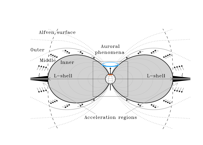
Figure 3: Meridional cross section of the dipolar dominated magnetosphere of a typical hot magnetic star. Beyond the Alfvén surface the magnetic field strength is not able to confine the ionized plasma pushed by the radiatively driven stellar wind (outer magnetosphere), with consequent formation of an equatorial magneto-disk surrounding the stellar magnetosphere, shaped like a mashed donut with a longitudinal thickness $l$. Closer to the star, the magnetic field is strong enough to confine the ionized gas and force it to co-rotate with the star (inner magnetosphere). The two magnetic field lines, pictured using solid lines (black: inner boundary; grey: outer boundary), locate the magnetospheric cavity (middle magnetosphere) where non-thermal electrons (evidenced by the small arrows), accelerated up to relativistic energies in the equatorial magneto-disk (black regions), produce radio emission by the incoherent gyro-synchrotron mechanism. Outside the Alfvén surface, the magnetic field topology (dotted lines) cannot easily be described by simple dipolar field lines. The box centered close to the star locates the deep magnetospheric regions where auroral phenomena can occur, including the coherent cyclotron maser (blue ring a few stellar radii above the poles) and the non-thermal X-rays from the auroral polar caps on the stellar surface (orange ring).

The acceleration of relativistic electrons is assumed to coincide with the magneto-disk, where magnetic reconnection events are expected to occur. This region is described as a thin equatorial disk of length $l$ and located beyond the last closed magnetic field line, corresponding to the distance $L$ where the last closed magnetic field line crosses the magnetic equatorial plane. It is expected that the magnetic field topology of this “unstable” magnetospheric region cannot be easily described with simple dipole magnetic field lines. However, we empirically observed that the contribution to the radio emission of the magnetospheric regions located far from the star and close to the magnetic equator is negligible, particularly at the intermediate and high frequency ranges (Sec. 3.3). The non-dipolar topology of the equatorial magneto-disk has then negligible effects on the calculation for non-thermal radio emission. In fact, the bulk of the non-thermal radio emission originates from magnetospheric regions at higher magnetic latitudes, regions that are likely well-described by the simple dipole topology. Hence, the dipole like magnetic shell where the relativistic electrons freely propagate is delimited by the two magnetic field lines of $L$ and $L+l$.

In modeling the non-thermal emission, we take the relativistic electron population to conform with an isotropic pitch-angle distribution (angle $\phi$ formed by the velocity direction with respect to the local magnetic field vector) and having a power-law energy distribution ($\propto E^{-\delta}$) with spectral index $\delta$. Up to the locations where the non-thermal emission is produced, the non-thermal electrons are assumed to freely propagate in vacuum, in accordance with the low density of the wind electrons (order of magnitude $10^{6}$ cm^-3 at the Alfvén radius), so the collisional energy loss mechanism is then negligible (Petrosian, 1985).

In the middle magnetosphere, the number density of non-thermal electrons is approximately constant. This arises because of two effects. First, the invariance of the magnetic moment of the gyrating electron ($\propto\sin^{2}\phi/B$) causes the magnetic mirroring effect on the electrons moving towards regions of increasing magnetic field strength, which results in a decreasing number of non-thermal electrons able to reach the deep magnetospheric regions. On the other hand, the solenoidal condition of the magnetic field causes a decreasing volume of the dipole-like flux tube as the magnetic field strength increases, balancing the decreasing number of the non-thermal electron when approaching the stellar surface. The result is a nearly constant number density ($n_{\mathrm{r}}$) of the non-thermal electrons responsible for the radio emission.

All the physical parameters needed for the calculation of the emission and absorptions coefficients for the gyro-synchrotron emission mechanism (Ramaty, 1969; Klein, 1987) are calculated within each grid point (i.e. the local magnetic field strength and its orientation). As the final step, before the integration of the radiative transfer equation, the spatial distribution of the thermal electron density trapped within the inner magnetosphere is estimated using the MCWS model, which assumes the density is linearly decreasing outward while the temperature is linearly increasing. The simple relationship: $T\propto r$ ($r$ radial distance), was deduced by Babel & Montmerle (1997) via modeling of the post-shock region in the case of fast rotating stars. Further, following the MCWS model, the thermal plasma pressure plus the wind ram pressure is constant. Far from the boundary shock the wind pressure becomes negligible, then in the post-shock region $n(r)T(r)=n_{0}T_{0}$, following the isobaric approximation. The thermal electron density at the stellar surface ($n_{0}$) is a free parameter, whereas the temperature there ($T_{0}$) is set to $T_{\mathrm{eff}}$. Our model accounts for free-free absorption from thermal electrons (Dulk, 1985). Then at a given radio frequency ($\nu$), we perform a numerical integration of the radiative transfer equation along the line of sight. The solution for a grid of such rays allows us to calculate the spatial distribution of the brightness and for a given stellar distance, the predicted flux from the unresolved source.

A model realization requires the following parameters: the equatorial radius of the magnetic shell where the relativistic electrons freely propagate ($L$); the thickness of the magnetic shell ($l$); the spectral index for the energy distribution of relativistic electrons ($\delta$); the number density of the relativistic electrons ($n_{\mathrm{r}}$); and for the thermal electrons trapped within the inner magnetosphere, the number density at the stellar surface ($n_{0}$). Note that Leto et al. (2017a) showed that $n_{\mathrm{r}}$ and $l$ are degenerate parameters, so that only the column density of the relativistic electrons ($n_{\mathrm{r}}\times l$) can be constrained.

3.2 Radio spectra calculation over broad spectral range

For each of the ten stars in the sub-sample, we calculated the non-thermal radio emission within the frequency range of 0.1–400 GHz. We adopted a spacing of $\Delta\log\nu=0.2$, corresponding to 19 different frequencies in the calculations, to evaluate time-averaged synthetic spectra. In particular, we analyzed the orientations corresponding to the two extrema of the effective magnetic field curves and to one null (if predicted by the corresponding ORM geometry, otherwise the intermediate phase between the extrema was calculated), for a total of 3 different rotational phases. These particular phases were appropriately identified from each individual star using the ORM parameters as listed in Table 2 (thus each star has 3 tailored calculations appropriate for the 3 phases identified).

To make this large computational effort possible, we restricted the exploration of parameter space to $L$ and $n_{\mathrm{r}}\times l$. The other parameters of the models were assumed close to the values retrieved by analyzing the individual stars already published (Trigilio et al., 2004; Leto et al., 2006, 2017a, 2018, 2020a, 2020b), having well-sampled single-frequency radio light curves, both for Stokes $I$ and $V$. In those cases, a fine-tuning of all the model parameters was performed to reproduce the observed light curve shapes. The previously published models have thermal electron density numbers determined at the stellar surface in the range 1–$5\times 10^{9}$ cm^-3 and spectral indices of the non-thermal electron energy distribution in the range 2–4. These values are fairly similar for all the previously analyzed stars. Consequently, for this paper we adopt: $n_{0}=3\times 10^{9}$ cm^-3 and $\delta=2.6$. For $n_{0}$ we used the average of the existing ranges of values. The adopted $\delta$ is the average of the values indirectly estimated for the few stars for which their X-ray spectra displayed a non-thermal photon component (Leto et al., 2017a, 2018; Pillitteri et al., 2018; Robrade et al., 2018).

To perform the broadband spectral analysis, the radio spectral calculations were obtained by varying the parameter $L$ in the range 8–20 R_∗ (with steps of $\Delta L=0.5$ R_∗, corresponding to 24 different magnetospheric sizes) and $n_{\mathrm{r}}\times l$ in the range $10^{15}$–$10^{17}$ cm^-2 (with steps of $\Delta\log(n_{\mathrm{r}}\times l)=0.05$, corresponding to 40 different cases). The total number of calculations is $\approx 5.5\times 10^{5}$. The spatial grid has different levels of resolution depending on its proximity to the star. We used narrow steps (0.1 R_∗) for distances below 8 R_∗; mid-sized steps (0.3 R_∗) for intermediate distances in the range 8–12 R_∗; and finally coarse steps (0.5 R_∗) at distances beyond 12 R_∗.

Table 2: Magnetosphere parameters used to calculate the stellar radio spectra shown in Fig. 2. Fixed parameters: $n_{0}=3\times 10^{9}$ cm^-3; $\delta=2.5$.

Star	$i$	$\beta$	$L$	$B_{L}$	$\dot{M}_{L}$	$n_{\mathrm{r}}\times l$	$\tilde{\chi}^{2}$
HD	(deg)	(deg)	(R∗)	(G)	(M⊙ yr-1)	($10^{15}$ cm-2)
36485a	$19$	$~{}~{}4$	$16$	$1.1$	$~{}~{}5.1\cdot 10^{-10}$	$3.5$	0.6
37017b	$39$	$57$	$13$	$1.4$	$~{}~{}5.9\cdot 10^{-10}$	$10$	0.7
37479b	$77$	$38$	$15$	$1.6$	$1.4\cdot 10^{-9}$	11.2	0.6
124224c	$46$	$76$	$12$	$1.1$	$~{}~{}1.5\cdot 10^{-10}$	1.6	0.8
133880d	$55$	$78$	$18$	$0.8$	$~{}~{}2.4\cdot 10^{-10}$	$3.5$	0.3
142184b	$64$	$~{}~{}9$	$10$	$4.5$	$1.2\cdot 10^{-9}$	56	0.5
142301a	$68$	$58$	$19$	$0.9$	$~{}~{}4.9\cdot 10^{-10}$	$2.8$	2
147932e	$74$	$~{}~{}5$	$13$	$3.0$	$1.3\cdot 10^{-9}$	6.3	0.04
147933f	$35$	$78$	$9$	$1.8$	$~{}~{}7.5\cdot 10^{-10}$	$2.8$	0.1
182180a	$53$	$82$	$14$	$1.7$	$~{}~{}7.7\cdot 10^{-10}$	11.2	0.2

• References of the stellar geometry: ^a Shultz et al., 2020; ^b Shultz et al., 2019b; ^c Kochukhov et al., 2014; ^d Bailey et al., 2012; ^e Leto et al., 2020b; ^f Leto et al., 2020a.

Finally, the grid of calculated spectra was used to find the best match to observations. For goodness of the spectral fit, we calculated the reduced chi-square statistical parameter, defined as $\tilde{\chi}^{2}=\chi^{2}/{\mathrm{d.\,o.\,f.}}$, where the degrees of freedom (d. o. f.) is equal to the number $n$ of the different observed frequencies minus the two free parameters of the model. The formulation ${\chi}^{2}=\sum_{i=0}^{n}(O_{i}-E_{i})^{2}/\sigma_{i}^{2}$ has been used, where $O_{i}$ is the measured flux (with the related uncertainty $\sigma_{i}$) and $E_{i}$ is the expected value from the calculation at the corresponding $i$-th frequency. For the evaluation of $\tilde{\chi}^{2}$, the calculated spectra have been interpolated to match the frequencies of the observations. To make the $\tilde{\chi}^{2}$ estimation reliable, we related to the radio measurements marked by the open symbols in Fig. 2 (spectral data provided by unique or few measurements) the average fractional error gained by the other measurements, in this way the dispersion of the measurements due to the rotational modulation of the radio emission is taken into account. Further, as it will be extensively discussed later, we suspect that the theoretical high-frequency radio emission suffers from critical model limitations, then, the high-frequency measurements ($\nu\gtrapprox 30$ GHz), when available, have not been taken into account when evaluating $\tilde{\chi}^{2}$. The calculated spectra superimposed with the observations are shown in Fig. 2.

Table 2 lists model parameters for the synthetic spectra that best fit the data, including the magnetic field strength ($B_{L}$) at $L$. Values of $\tilde{\chi}^{2}$ (Table 2) are always lower than 1 (or close to 1 in the case of HD 142184). Our new spectral calculations recover parameters that are fairly similar to what had been obtained for stars that had previously been modeled in terms of rotational modulations. This is encouraging since here we are modeling spectra whereas before the emphasis was on light curves, and suggests that our approach produces consistent and reliable results. Overall, calculations for these 10 stars indicate that on average, the relativistic electrons are injected at a distance of $\langle L\rangle=14\pm 3$ R_∗, and the local magnetic field strength is $\langle B_{L}\rangle=2\pm 1$ G.

3.3 The broadband radio spectra

The calculated radio spectra at $\nu\lessapprox 30$ GHz for the ten magnetic stars in our sub-sample are quite independent of their stellar parameters. The spectral shapes suggest the existence of both low- and high- frequency cutoffs, in accordance with the observations. Early B and late A magnetic stars have almost indistinguishable radio spectra (Fig. 2). The small differences are mainly related to the individual magnetospheric geometries. The nearly universal spectral behavior can be summarized as follows: the radio flux increases with increasing frequency (at low-frequency); then the radio spectrum becomes almost flat (at intermediate-frequency); and finally the model spectrum has a negative slope (at high-frequency), although in some cases a clear high-frequency emission peak was predicted by our calculations.

To better understand the overall spectral behavior, we computed the spatial distribution of the radio emission from a typical dipole-dominated magnetic star. The synthetic radio maps have been obtained at low-, intermediate-, and high-frequency ranges. The three panels of Fig. 4 show the synthetic radio maps for these three radio regimes. The three calculated frequencies are respectively: low frequency ($\nu=2$ GHz); intermediate frequency ($\nu=6$ GHz); and high frequency ($\nu=100$ GHz). We used HD 142184 as a template, with a polar field strength of $B_{\mathrm{p}}=9$ kG. The radio maps clearly highlight the spatial location within the middle-magnetosphere of the regions that mainly contribute to the emission at a given frequency range.

• Low frequency behavior. The low-frequency side of the radio spectrum tracks the radio emission arising from the furthest regions of the middle-magnetosphere: see the top panel of Fig. 4. As previously explained (see Sec. 3.1), each grid point of the 3D model is a cube-shaped homogeneous source characterized by a typical gyro-synchrotron radio spectrum peaked at the turnover frequency, which is proportional to the local magnetic field strength (Dulk & Marsh, 1982). The positive slope of the radio spectrum at the low-frequency regime, observed and calculated, is due to the grid points, that should have contributed mainly to the low-frequency emission, being external to the middle-magnetosphere and are not crossed by relativistic electrons. Hence, far from the star, the magnetospheric regions that should mainly radiate at low-frequencies ($\nu\lessapprox 1$–2 GHz), and where the local magnetic field strength is low (typically less than a few gauss), fall outside the middle-magnetosphere. These outer regions do not contribute to the non-thermal radio emission, preventing also to further investigate for the possible effects of the non dipolar topology of the equatorial magneto-disk on the calculation of the radio emission.

  

  

  

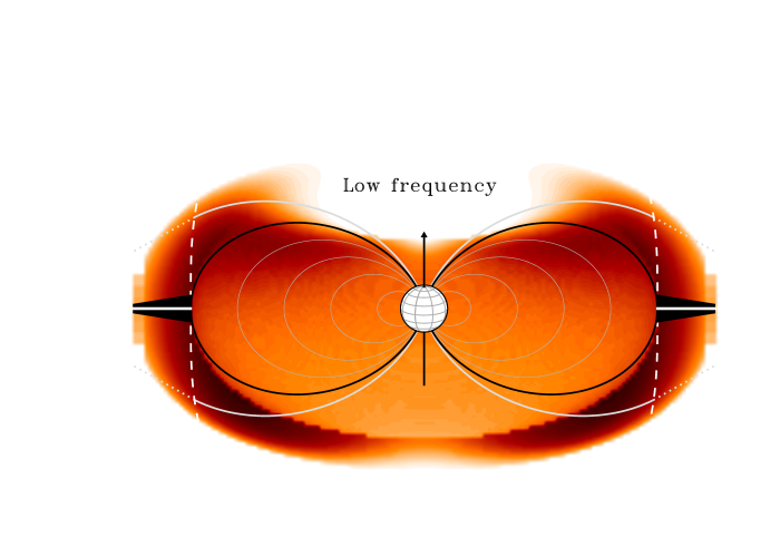
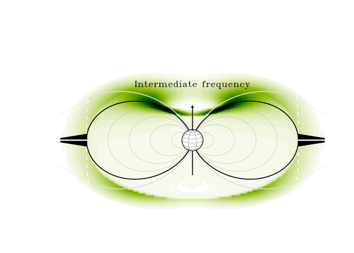
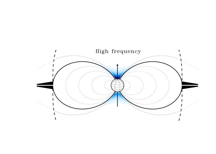
  Figure 4: Synthetic brightness spatial distributions evaluated at three representative radio frequencies computed for the parameters of the template star HD 142184. Top panel: low frequency behavior (red, $\nu=2$ GHz). Middle panel: intermediate frequency behavior (green, $\nu=6$ GHz). Bottom panel: high frequency behavior (blue, $\nu=100$ GHz). In all panels, the dashed line demarcates the Alfvén surface (white lines in top and middle panels, black line in the bottom panel).

• Intermediate frequency behavior. The radio emission produced at this frequency range ($\approx 2$–30 GHz) has the optimal tuning for non-thermal radio emission from a dipole-dominated magnetosphere. In fact, the frequency peaks of the elementary spectra produced by each homogeneous element sampling the middle magnetosphere fall within this spectral range. The synthetic radio map reveals that the brighter source regions are located far from the middle-magnetosphere boundaries, either near the stellar surface or near the Alfvén surface (see the middle panel of Fig. 4). The nearly flat spectra, which characterize the intermediate frequency behavior, is qualitatively understood when taking into account that the brighter magnetospheric regions close to the star (where the magnetic field is stronger) have less volume than the more distant low brightness regions, where the emission at the lower radio frequencies mainly originates.

• High frequency behavior. Radio emission at higher frequencies ($\gtrapprox 30$ GHz) originates from the deep magnetospheric regions close to the star (see the bottom panel of Fig. 4). In this frequency regime the negative slope of the spectrum is the obvious consequence of the radiating regions that meet the stellar surface. The decaying of the high-frequency flux has the same qualitative explanation as the flux drop occurring when the radio frequency decreases, which is that the magnetospheric regions that should have been mainly responsible for radio emission at very high (and low) frequencies fall outside the middle-magnetosphere. Further, the high-frequency side of the radio spectrum might also be strongly affected by the plasma processes responsible for auroral phenomena (i.e., possible plasma evaporation as a consequence of non-thermal auroral X-ray emission), which is plausibly always occurring for all magnetospheres in these kinds of stars. This might be a critical issue for high frequency radio emission. In practice, the adopted model conditions may not be valid within deep magnetospheric regions where high-frequency emission originates (i.e., the spatial distribution of the non-thermal electron density might be inhomogeneous). The topic will be a matter of future study, mainly focused on the high-frequency side of the radio spectrum of such stars. At present, the limited available radio measurements prevent further investigation of the physical conditions occurring within the deep magnetospheric regions. The calculated radio light curves at the high-frequency spectral range are shown using only dotted lines in Fig. 2.

The comparison between observations and calculations shows excellent accord at the low and intermediate frequency ranges (Fig. 2). At the higher frequency side of the radio spectra, the few available observations (see Appendix A for details) are not sufficient to assert any firm conclusions regarding high-frequency spectral behavior, nor reliable estimates of the high frequency cutoff. The evident large discrepancies between calculations and observations require further investigation. In practice, possible plasma effects related to auroral phenomena might significantly affect the emission level and the rotational modulation of high-frequency radio emission. This possibility drives the need for a much better sampling of the entire stellar rotation period for a larger sample of stars to determine the average high-frequency spectral behavior.

Despite some modeling limitations, particularly at high-frequency, the capability to reproduce the spectral behavior at low and intermediate frequencies allows us to place strong constraints on the spatial location for the acceleration of the non-thermal electrons. From a qualitative point of view, once all the magnetosphere parameters have been fixed, the radio spectrum from a large magnetosphere (large $L$) is characterized by a turn-over, namely the narrow spectral region where the change from the rising to the flat regime of the radio spectrum occurs, situated at low frequency. Conversely, the radio spectrum from a smaller magnetosphere (small $L$) has its turn-over located at a higher frequency.

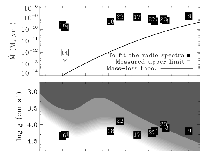
Figure 5: Top panel: theoretical wind prediction of Krtička (2014) (solid line) compared with the mass loss rate from modeling of the radio spectra listed in Table 2 (black squares). The numbers within squares correspond to object in Table 1. The open square represents the upper limit estimation of the wind from HD 124224. Bottom panel: location of the sub-sample stars on the $\log g$ vs. $T_{\mathrm{eff}}$ diagram. The shaded areas indicate different wind regimes, according to Babel (1996) and Hunger & Groote (1999). The wind regions have been taken from Fig. 6 of Babel (1996) and Fig. 1 of Hunger & Groote (1999). Dark gray locates the homogeneous wind region; light gray locates where the expected wind is inhomogeneous; the white area corresponds to the static atmosphere.

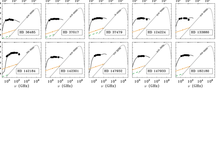
Figure 6: Black line: gyro-synchrotron spectra already shown in Fig. 2; grey line: black-body spectra obtained using the stellar parameters listed in Table 1; orange dotted line: wind spectra calculated using the relation given by Scuderi et al. (1998) and adopting the spherical mass loss rate listed in Table 2; green dashed line: wind spectra calculated using the theoretical wind (Krtička, 2014), the expected wind spectra of some stars are lower than the black-body emission. Filled bullets are the radio measurements, filled gray diamonds represent the WISE and 2MASS infrared measurements.

4 The role of the wind

4.1 Indirect estimation of the wind

The MCWS paradigm successfully explains many observational features of the early-type magnetic stars, from the radio to the X-ray regime (Babel & Montmerle, 1997). In particular, the thermal X-ray emission from the magnetically confined wind is produced by the strong shock occurring close to the magnetic equatorial plane (ud-Doula et al., 2014). Following the Rankine-Hugoniot condition, the temperature of the X-ray radiating plasma ($T_{\mathrm{X}}$) is related to the velocity of the colliding wind streams ($v_{\mathrm{wind}}$) arising from the stellar hemispheres with opposite magnetic polarity by the relation $T_{\mathrm{X}}\approx 14(v_{\mathrm{wind}}/10^{3}\,{\mathrm{km\,s^{-1}}})^{2}$ MK. Approximating $v_{\mathrm{wind}}$ with $v_{\infty}$, the terminal wind velocity can be indirectly constrained by the measured temperature of the thermal plasma emitting X-rays, that is $T_{\mathrm{X}}\approx 10$ MK (Oskinova et al., 2011; Pillitteri et al., 2016, 2017; Leto et al., 2017a, 2018; Robrade et al., 2018). The corresponding value of the terminal wind velocity is $v_{\infty}\approx 900$ km s^-1, that is reasonable for main sequence B type stars (Prinja, 1987).

In the paradigm associated with wind magnetic confinement, non-thermal acceleration is placed at the equatorial Alfvén radius. The $L$-shell parameter from our models (Sec. 3.2) can be used as an indirect estimate of $R_{\mathrm{A}}$. Thus, we can quantify the spherical wind of the stars analyzed in Sec. 3 by equating the kinetic energy density of the wind (ram pressure plus centrifugal component) to the magnetic energy density: $p_{\mathrm{ram}}+1/2(\rho\omega^{2}d^{2})=B^{2}/8\pi$, where $\rho$ is the wind density, $\omega$ is angular rotation speed, and $d$ the distance of a generic point located on the magnetic equatorial plane from the rotation axis. As a consequence of the ORM geometry the equatorial Alfvén radius is a function of the magnetic longitude (Trigilio et al., 2004). Comparing the longitudinal average of $R_{\mathrm{A}}$ with the $L$-shell size of the individual stars required to reproduce the measured radio spectra, we indirectly derive the mass loss rate of the spherical wind ($\dot{M}_{\mathrm{L}}$) that is able to exceed the magnetic tension at the appropriate distance to originate a radio emitting magnetosphere that reproduces the spectrum. The values of $\dot{M}_{\mathrm{L}}$ thereby derived for the individual stars are listed in Table 2. The mass loss rates are in the range $10^{-10}$–$10^{-9}$ M_⊙ yr^-1.

4.2 Comparison with the theoretical wind

The stars analyzed in Sec. 3 have effective temperatures ranging from $\approx 12$–23 kK. The effective temperature has a primary effect on the radiatively driven stellar wind. However, the radio spectra of our sample stars are well reproduced with similar values of the magnetic shell size $L$ (Sec. 3.2), hence, no correlation seems to exist between $L$-shell and $T_{\mathrm{eff}}$.

Estimated values of the mass loss rate ($\dot{M_{\mathrm{L}}}$ listed in Table 2) for the spherical winds of non-magnetic counterparts to the individual stars of our sub-sample are shown in the top panel of Fig. 5, as a function of the corresponding effective temperature. The rather limited spread in wind mass-loss rates as estimated from the radio spectral models stands in substantial contrast with values expected from radiative wind driving, mainly owing to the rather large spread in stellar temperatures and consequently luminosities of the sub-sample. As an example, consider HD 147933, with a luminosity $L_{\ast}\approx 4000$ L_⊙ (Pillitteri et al., 2018) as opposed to HD 133880, with $L_{\ast}\approx 80$ L_⊙ (Netopil et al., 2017). Hence, HD 147933 is about 2 orders of magnitude brighter than HD 133880. According to the CAK (Castor, Abbott & Klein, 1975) framework of the radiatively driven wind acceleration, the expected mass-loss rate is related to the stellar luminosity as $\dot{M}\propto L_{\ast}^{1/\alpha}$, with $\alpha\approx 0.6$ (Puls et al., 2008; ud-Doula et al., 2014), the expected mass-loss rate from HD 147933 would be about 3 orders of magnitudes higher than for HD 133880. Further, there is a large discrepancy between the mass loss rates empirically estimated from radio (reported in Table 2) and those predicted theoretically. Krtička (2014) theoretically derived the dependence of mass-loss rates on $T_{\mathrm{eff}}$ for BA-type dwarfs, given by the relation: $\log\dot{M}=a+bT_{4}+cT_{4}^{2}$, with $T_{4}=T_{\mathrm{eff}}/(10^{4}\,{\mathrm{K}})$, and where $a=-22.7$, $b=8.96$, and $c=-1.42$. Their predictions are in good agreement with the empirically derived $\dot{M}$ of magnetic B-type stars (Oskinova et al., 2011). Considering the top panel of Fig. 5, the $\dot{M}$ required to reproduce the radio spectra (see Sec. 4.1) are significantly higher than expected, with the gap widening at lower $T_{\mathrm{eff}}$. The discrepancy is especially large at the lowest $T_{\mathrm{eff}}$ corresponding to Ap stars. For instance, for a template A0p star, CU Vir (HD 124224), Krtička et al. (2019) derive the upper limit $\dot{M}=10^{-12}\,M_{\odot}$ yr^-1, which is orders of magnitude lower than that required by our radio spectra models.

To further investigate the physical conditions in atmosphere of our sample stars, in the bottom panel of Fig. 5 we indicate the positions of stars in our sub-sample on the $\log g/T_{\mathrm{eff}}$ diagram. The surface gravity ($\log g$) was retrieved from the literature for the individual stars (Bailey et al., 2012; Grunhut et al., 2012; Rivinius et al., 2013; Alecian et al., 2014; Kochukhov et al., 2014; Pillitteri et al., 2018; Shultz et al., 2019a). The values of $\dot{M}$ for main sequence B-type stars has been theoretically predicted by Babel (1996), who recognized three wind regimes, namely: a homogeneous wind; a chemically inhomogeneous wind; and static atmosphere. These three wind regimes depend on the combined effects of temperature and surface gravity. Based on results from Fig. 1 of Hunger & Groote (1999), the qualitative effect of chemical anomalies is roughy to shift down the lower boundary curve taken from Fig. 6 of Babel (1996). In the bottom panel of Fig. 5 the down-shifted curves are pictured using the light grey with a gradually decreasing intensity.

The location on the $\log g/T_{\mathrm{eff}}$ diagram of the ten stars from our sub-sample is in accordance with the mass loss recipe of Krtička (2014). Note that about $85\%$ of the stars in our complete sample have $T_{\mathrm{eff}}\lessapprox 20$ kK, in which case only weak metallic ($\dot{M}\lessapprox 10^{-14}$ M_⊙ yr^-1) winds are expected (Babel, 1996). Accounting for the corresponding magnetic field strength, we expect Alfvén radii larger than the average value retrieved by calculating the synthetic spectra ($R_{\mathrm{A}}\approx 14$ stellar radii).

In late B and early A stars, the inhomogeneous (hydrogen-free) weak wind (Babel, 1995, 1996) would continuously deposit a small amount of metal ions into their centrifugally supported magnetospheres. The secular accumulation of trapped ionized material eventually fills the magnetosphere. The density distribution of the magnetically confined circumstellar plasma around hot magnetic stars has been theoretically studied by Preuss et al. (2004) and Townsend & Owocki (2005). The thermal plasma accumulated by the wind at low magnetic latitudes might be the cause of significant departures from the simple dipole topologies. Far from the star, the magnetic tension might no longer be able to confine this thermal material, leading to centrifugal breakout (ud-Doula et al., 2006), with consequent local magnetic reconnection that is likely a source of plasma acceleration. Shultz et al. (2020) and Owocki et al. (2020) have demonstrated that the onset, emission strength scaling, and line profile morphologies of H$\alpha$ emission from centrifugal magnetospheres can only be explained if mass-balancing is achieved by continuous centrifugal breakout events occurring at small spatial scales throughout the centrifugal magnetosphere.

4.3 The wind spectra and the stellar SEDs

To further investigate the wind mass loss from early-type magnetic stars, we have taken into account possible effects due to the ionized material carried out by the radiatively driven stellar wind. We compared the wind thermal emission with the corresponding non-thermal radio emission. Both wind regimes discussed in Sec. 4.2 have been analyzed. Further, we extended to the radio regime the expected emission from the stellar surface modeled by a simple black-body spectrum.

Radio emission from stellar winds was theoretically studied under simplified assumptions. The radio flux of a spherical wind increases as a function of the frequency like $S_{\nu}\propto\nu^{0.6}$ (Wright & Barlow, 1975; Panagia & Felli, 1975). In Appendix C the equation of the wind spectrum is explicitly reported (Eq. 2). The wind spectra calculated using Eq. 2 and adopting the indirect estimation of the spherical wind of the individual stars ($\dot{M}_{L}$ listed in Table 2) are shown in Fig. 6, pictured by the orange dotted lines. Looking at the figure, it is clear that the expected wind radio emission from the B/A magnetic stars analyzed here is faint. The wind spectra cover almost the same spectral range of the non-thermal radio emission, but are orders of magnitudes less bright.

For the ten stars analyzed in Sec. 3, the spectral energy distributions (SED), from the radio to the UV domain, have been calculated combining the radio spectra (Sec. 3.2) and the blackbody spectra ($T_{\mathrm{eff}}$ listed in Table 1) radiated from the surface scaled at the stellar distance. In the figure, the radio and infrared measurements have also been reported. To minimize for possible absorption effects, interstellar or intrinsic, we collected near- and mid-infrared measurements, from the Two Micron All Sky Survey (2MASS) (Cutri et al., 2003) and the Wide-field Infrared Survey Explorer (WISE) (Cutri et al., 2014) catalogues; these measurements are shown in Fig. 6.

The wind spectra corresponding to the theoretical radiative wind mass-loss rates, expected on the basis of the corresponding stellar temperatures, have been calculated too. As expected by the low level of the theoretical radiative wind from B/A spectral type stars, the wind spectra are much fainter (green dashed lines shown Fig. 6). In some cases the wind mass loss rate is so low as to radiate less than the black-body radiation of the stellar surface, at the radio spectral range analyzed. In these cases the corresponding wind spectra have not been shown.

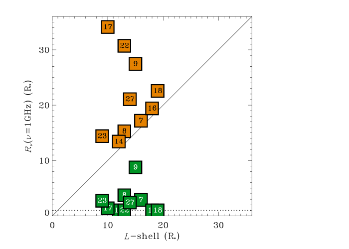
Figure 7: Radii of the radio photosphere calculated at the representative frequency $\nu=1$ GHz as a function of the corresponding magnetospheric size ($L$-shell) required to reproduce the radio spectra of the non-thermal radio emission. The $R_{\nu}$ values have been derived in two cases: assuming the wind mass loss rate theoretically expected (green symbols); and assuming the $\dot{M}_{L}$ required to break the stellar magnetic field lines at the distance equal to the $L$-shell (orange symbols). The dotted line locates the lower limit of $R_{\nu}$, coinciding with the stellar radius. The solid line separates the case of a wind radio photosphere that incorporates the region radiating non-thermal radio emission (upper left) from the case where the wind emitting region is located inside (bottom right).

The early type magnetic stars are surrounded by large scale dipole-like magnetic field, in this case the spherical wind assumption is a rough schematization of the real case. In fact, the wind material can be lost from the polar caps only, where the magnetic field lines are open. At the lower magnetic latitudes, the wind is trapped and channeled by the closed field lines. The radiative wind in presence of magnetic field produces the typical observable features, from the X-ray to the radio, successfully explained by the MCWS model.

The effective wind mass loss rate of the early-type magnetic stars is expected lower than a simple spherical wind. Therefore, it is plausible to expect that the spherical wind assumption produce overestimated effects. In any case, also adopting the simplified spherical assumption, the wind emission is never comparable to the emission level of the non-thermal radio emission produced by the MCWS model. The ionized matter released by the polar caps might produce frequency-dependent absorption effects for the non-thermal radio emission. The theory of spherical stellar winds predicts that each radio frequency of the wind spectrum arises from a well-constrained emitting region, similarly to a radio photosphere where the optical depth is $\tau\approx 0.4$ (Panagia & Felli, 1975). The radio photosphere location is a function of the observing frequency, with the radius of this emitting region decreasing as the frequency increases, in accordance with the relation $R_{\nu}\propto\nu^{-0.7}$. Adopting the spherical wind simplified assumption, the dependence of the size of the wind-emitting region on the mass-loss rate and on other stellar parameters is explicitly reported in Eq. 3. The high frequency cutoff of the wind spectrum is defined by the frequency radiated from the wind region that meets the stellar surface.

To account for possible absorption effects, we calculated the size of the wind radio photosphere at $\nu=1$ GHz. We chose this frequency because the bulk of the non-thermal radio emission is produced at $\nu>1$ GHz. The radii of the radio photosphere as a function of the size of the magnetosphere ($L$-shell parameter) where the non-thermal radio emission arises are shown in Fig. 7. The $R_{\mathrm{\nu=1\,GHz}}$ values have been calculated for each star for both wind regimes: the $\dot{M}$ theoretically expected from the stellar temperatures; and the $\dot{M}_{L}$ indirectly derived from the non-thermal spectra (listed in Table 2). Looking at Fig. 7 it is evident that the radio photosphere calculated using $\dot{M}$ is contained within the non thermal emitting region, making any possible absorption effect negligible.

The non-thermal radio spectra calculations have been performed under the assumption that, outside the middle-magnetosphere, the absorption effects of thermal plasma can be neglected. This corresponds to assuming the electromagnetic waves propagate in vacuum. The accordance between the observed and the calculated spectra support this assumption. It follows that the negligible absorption effect predicted by the weak wind regime is in accordance with our model assumption. This is a further evidence that the mass loss rate values indirectly derived from the non-thermal radio emission ($\dot{M}_{L}$) are unreliable.

5 Is radio emission age-dependent?

As discussed in Sec. 4, the over-simplified assumption that the size of the radio emitting magnetosphere coincides with the Alfvén radius has something wrong. If the wind is the plasma source which continuously accumulates within the inner magnetosphere, then, non-thermal radio emission from early-type magnetic stars might be potentially related to the stellar age. As suggested in Sec. 4.2, the wind plasma accumulation produces centrifugal breakout events (Shultz et al., 2020; Owocki et al., 2020) that might make the corresponding stellar magnetosphere radio-loud.

To search for a possible age dependence, the measured radio luminosities are shown in the top panel of Fig. 8 as a function of the corresponding fractional main sequence age (as listed in Table 1). The stars earlier than spectral type B8 have been marked using blue symbols, while red symbols have been used for cooler stars. Looking at the top panel of this figure, no significant relation appears evident between the stellar radio luminosity and corresponding stellar age for the hotter stars, whereas a possible decaying trend is suggested for the cooler stars. This effect resembles the results obtained by Fossati et al. (2016), moreover this closely matches to the behavior of the H$\alpha$ emission discovered by Shultz et al. (2020). Studying a large sample of massive and hot main sequence magnetic stars, Fossati et al. (2016) found that large-scale magnetic fields suffered a time-dependent decaying trend, effect that was further confirmed by Shultz et al. (2019c). In particular, the magnetic flux $\Phi$ ($=B_{\mathrm{p}}R_{\ast}^{2}$) decreases more steeply than expected from the magnetic flux conservation law, as predicted by the expansion of the stellar radius along the MS evolution. Further, Sikora et al. (2019a) indicated that the chemical surface composition of early type magnetic stars is strictly related with the stellar age, particularly for the cooler stars.

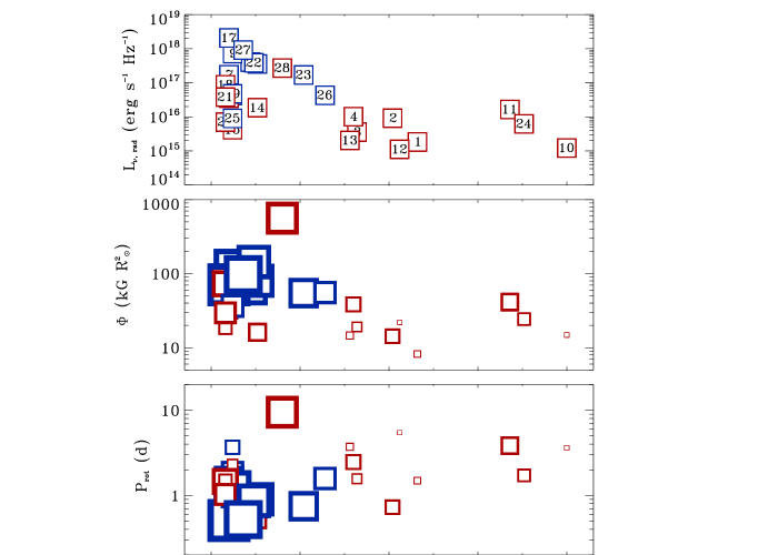
Figure 8: Top panel: Radio luminosities as a function of the fractional main sequence age, where blue symbols refer to stars earlier than B8 and red symbols to the cooler stars. Middle and bottom panels show magnetic fluxes the rotation periods as a function of fractional age. The size of the symbol is proportional to the radio luminosity of the individual star.

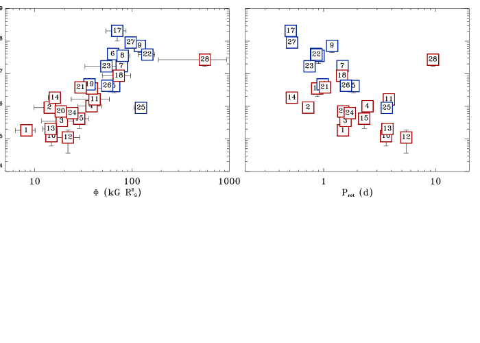
Figure 9: Left panel: the radio luminosity as a function of the magnetic flux ($\Phi$). Right panel: radio luminosity as a function of the rotation period ($P_{\mathrm{rot}}$). The blue symbols refer to the hot stars, and the red to the cooler stars (SP$>$B8).

Although the sample of early-type magnetic stars analyzed here is small, we have searched for possible age-dependent effects on the magnetic flux and the stellar rotation. As already well studied in this class of stars, the stellar rotation period is expected to increase dramatically over time (Sikora et al., 2019b; Shultz et al., 2019c). In the middle and bottom panels of Fig. 8, we show $\Phi$ and $P_{\mathrm{rot}}$ as a function of the fractional main sequence stellar age. The corresponding stellar radio luminosity is indicated by the symbol size. For the hotter stars, the two analyzed stellar parameters do not show any significant age-dependent effects, whereas the magnetic field survives on the colder stars. Among the small sample of stars here analyzed, at young ages all magnetic field strengths are possible, but at old ages, there are few stars with strong fields, in particular, the older stars in our sample are also cooler stars (see Fig. 8). The same trends seem to be confirmed by the radio. In fact, there is a dearth of both old and strong radio emitters.

The large-scale magnetic fields of the early-type magnetic stars might significantly affect the stellar evolution. Shultz et al. (2019c) performed an extensive study on the dependences of the stellar magnetic flux as a function of various stellar parameters. They conclude that massive stars show a more pronounced magnetic flux decreasing with the age. Further, magnetic braking effects significantly reduce the stellar rotation period during the star’s life.

Although the small number of magnetic stars known as radio sources may introduce a selection bias, and a large fraction of stars in our sample have similar ages, their range of radio luminosities are fairly broad (see top panel of Fig. 8). This suggests that any connection between radio emission, magnetic field strength, rotation period, and age is not simple. The only relevant effect which emerged from the analysis of our small sample is the possible rough dependence of the radio luminosity with the magnetic flux and rotation period shown by the stars having similar ages. In particular, stars with a short rotation period and a high magnetic flux produce stronger radio emission (see middle and bottom panels of Fig. 8).

6 The effect of the rotating dipole

As discussed in Sec. 4, the wind is not the lead actor in the production of non-thermal radio emission. By contrast there may be a possible dependence on other stellar parameters that mainly characterize the rotation of the dipole-like magnetic field (Sec. 5).

The sample analyzed in this paper has heterogenous parameters. To well characterize the magnetic properties of the sample, a reliable parameter is the magnetic flux ($\Phi=B_{\mathrm{p}}R_{\ast}^{2}$), which combines both the effects due to the magnetic field strength and the stellar size. In the two panels of Fig. 9, the stellar radio luminosities are displayed as a function of $\Phi$ (left panel) and $P_{\mathrm{rot}}$ (right panel). The obvious trends seen in Fig. 9, confirm the dependence of radio emission on these two parameters. In particular, $L_{\nu,\mathrm{rad}}$ has a positive dependence with $\Phi$ and a negative one with $P_{\mathrm{rot}}$. These trends suggest identifying a parametrization that incorporates both these two parameters. The obvious way is to take their ratio.

In Fig. 10 the radio luminosities of the magnetic stars are reported as a function of what we are calling the “magnetic flux rate”, ${\Phi}/{P_{\mathrm{rot}}}$ (kG R${}_{\odot}^{2}$ d^-1). Already visual inspection of Fig. 10 reveals a strong correlation. To quantify the correlation, we calculated the Pearson correlation coefficient ($r$) and the Spearman’s rank correlation coefficient ($r_{\mathrm{s}}$). The $r$ statistical parameter is only sensitive to a linear relationship, whereas $r_{\mathrm{s}}$ is sensitive to any possible monotonic relation between the two analyzed variables. These two statistical parameters range between $-1$ and 1, with absolute values $\approx 0.7$, or higher, indicating a high correlation.

The correlation parameters indicated that the radio luminosity is strongly correlated to the ratio of magnetic flux to rotation period. In particular, $r\approx 0.75$ and $r_{\mathrm{s}}\approx 1$, suggesting that a non-linear relation exists. The scaling relation that best fits the data is:

$$L_{\nu,\mathrm{rad}}=10^{\alpha}\left(\frac{B_{\mathrm{p}}}{{\mathrm{kG}}}\right)^{\beta}\left(\frac{R_{\ast}}{{\mathrm{R_{\odot}}}}\right)^{2\beta}\left(\frac{P_{\mathrm{rot}}}{\mathrm{d}}\right)^{-\beta}(\mathrm{erg}~{}\mathrm{s}^{-1}~{}\mathrm{Hz}^{-1})$$ (1)

with $\alpha=13.6\pm 0.1$ and $\beta=1.94\pm 0.07$.

It is worth noting that following the Faraday-Lenz law, the empirical parameter $\Phi/P_{\mathrm{rot}}$ has the physical dimension of an electromotive force (e.m.f.$=-d{\Phi}/d{t}$). Even if in a co-rotating reference frame the stellar magnetic flux is not expected to be variable over time: a spinning dipolar magnetosphere has close similarities with Faraday disk dynamo, where the rotation of a conductive disk within a stable magnetic field, having the magnetic vector orientation aligned with the disk rotation axis, produces an e.m.f. (see experiments of Müller, 2014). We analyze the rotating magnetospheres from a reverse point-of-view. In a reference frame anchored to a free test charge located in the equatorial plane, with distance $R$ from the rotation axis, the magnetic field lines will be seen moving at velocity $v=\omega R$ ($\omega=2\pi/P_{\mathrm{rot}}$ rotational angular frequency). Assuming the ideal case of aligned dipole and spin axes, the magnetic and equatorial planes are coinciding. Then in the magnetic equatorial plane the magnetic field vectors are orthogonal to the plane and also to the velocity vector. Assuming the simplified homogeneous magnetic field condition, it follows that the test charge located at the stellar equator embedded within a homogeneous field (strength $B_{\mathrm{eq}}$) will be subjected to an induced electromotive force (Jackson, 1962) ${\mathrm{e.m.f.}}=-d{\Phi}/d{t}=\oint{\bf v}\times{\bf B}\,{d}{\bf l}$, that under the above simplified conditions can be written as: ${\mathrm{e.m.f.}}=\int_{0}^{R_{\ast}}v\,B_{\mathrm{eq}}\,{d}r=\int_{0}^{R_{\ast}}\omega\,r\,B_{\mathrm{eq}}\,{d}r=1/2\omega B_{\mathrm{eq}}R_{\ast}^{2}$ ($\propto\Phi/P_{\mathrm{rot}}$), (for details see Müller, 2014). Note that for a real magnetized plasma, the free charged particles cannot cross the magnetic field lines. The spinning stellar dipole plunged in the magnetospheric plasma can be treated following an ideal magnetohydrodynamic approach. The above discussion is only used to illustrate that a spinning dipole may be a source of electric voltage, potentially able to originate electric currents. In fact, in astrophysical applications, the electrodynamics of spinning dipoles have been the subject of many theoretical studies (Goldreich & Lynden-Bell, 1969; Goldreich & Julian, 1969; Ruderman & Sutherland, 1975).

The rough schematization performed above may be useful to perform order of magnitude relation between astrophysical observables (i.e. the radio luminosity) and general stellar parameters (i.e. the the stellar rotation period, the radius, and the magnetic field strength). In fact, the relation $\omega B_{\mathrm{eq}}R^{2}_{\ast}$, that resemble an electromotive force, is a useful scaling parametrization for the realistic electrodynamics of spinning magnetospheres. The stars analyzed in this paper typically have a dipolar magnetic field topology, with $B_{\mathrm{eq}}=B_{\mathrm{P}}/2$. Thus, the empirical parameter $\Phi/P_{\mathrm{rot}}$ can be easily transformed to the physical parameter $\omega B_{\mathrm{eq}}R_{\ast}^{2}$. If the rotation period is given in seconds, the equatorial magnetic field strength in Tesla, and the stellar radius in meters, the parametric electromotive force (named e.m.f.^∗) has the physical unit of Volts. In Fig. 11, the stellar radio luminosities are now reported as a function of the corresponding values of e.m.f.^∗ and given in unit of $10^{6}$ V. The e.m.f.^∗ is not the true electromotive force acting within the stellar magnetosphere (its study is out of the scope of this paper) but this is rather a useful parameter with which to quantify the capability of rotating magnetospheres for producing electric currents.

7 Other ordered magnetospheres

To test whether the result reported in Sec. 6 holds only for the early-type magnetic stars or if it is also valid in a wider context, we analyzed the incoherent radio emission from other types of stars (and one planet) characterized by large-scale and well-ordered magnetospheres, that are mainly described by a simple dipole magnetic field topology.

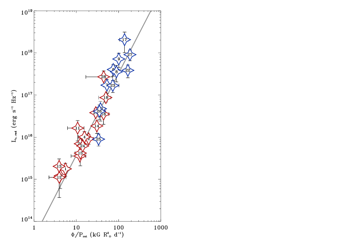
Figure 10: Radio luminosity of the early-type magnetic stars as a function of the ratio $\Phi/P_{\mathrm{rot}}$. The solid grey line is the power-law that best fits the two parameters. As in Figs. 8 and  9, the blue symbols refer to the hot stars, while the red symbols refer to the cooler stars (SP$>$B8).

7.1 The Case of Jupiter

The giant planet Jupiter is surrounded by a large-scale (almost dipolar) magnetic field, with the dipole axis nearly aligned with the planetary rotation axis (tilt angle $\approx 10^{\circ}$). Compared to the hot magnetic stars, Jupiter has a weak magnetic field, with $B_{\mathrm{J}}\approx 4.17$ G at the equator (Connerney et al., 2018), corresponding to $B_{\mathrm{P}}\approx 0.008$ kG. Jupiter is surrounded by ionized matter that comes from the volcanic moon Io (Io plasma torus) or captured from the Solar wind, which is affected by the planetary magnetic field out to a large distance (tens of Jupiter radii).

The jovian magnetosphere is a site of plasma phenomena responsible for Jupiter’s radio emission, which has been well-studied using ground-based observing facilities and radiometers onboard spacecrafts. Its radio spectrum is dominated at the low-frequency side by coherent auroral radio emission (Zarka, 2004), and at high frequencies ($\nu\gtrapprox 10$ GHz) by the black body thermal emission of Jupiter’s atmosphere. At intermediate frequencies, the incoherent synchrotron emission is another component of Jupiter’s radio spectrum. The multi-wavelength VLA images of the planet Jupiter show the spatial distribution of the non-thermal radio emission component from Jupiter (de Pater, 1991). This non-thermal component originates from the inner radiation belt located at $L<5$ Jupiter radii, inside the orbit of the moon Io.

The non-thermal radio component was disentangled from the thermal one and the wide band non-thermal jovian radio spectrum was discussed by de Pater (2004). We note that the spectral shape qualitatively resembles the overall behavior of the radio spectra of early-type magnetic stars (see Fig. 2), but is tuned at lower frequencies. The reference frequency of the Jupiter’s incoherent non-thermal emission is in fact $\approx 1.6$ GHz. The average luminosity of the incoherent radio emission is $L_{\nu,{\mathrm{rad}}}=1.8(0.4)\times 10^{6}$ erg s^-1 Hz^-1, obtained from scaling the multifrequency fluxes measurements to the distance from Earth of 4.04 a.u (de Pater et al., 2003; de Pater & Dunn, 2003).

Jupiter’s equatorial radius and magnetosphere rotation period are $R_{\mathrm{J}}=71492$ km and $P_{\mathrm{J}}=9$ h 55 min 29 s. In MKS unit, the effective electromotive force (as defined in Sec. 6) produced by the rotation of the Jupiter’s magnetosphere is ${\mathrm{e.m.f.}^{\ast}}=376$ MV. This coincides with the magnetic potential energy available from the jovian magnetosphere’s corotation, defined by Khurana et al. (2004) as $\omega_{\mathrm{J}}B_{\mathrm{J}}R_{\mathrm{J}}^{2}$ (with $\omega_{\mathrm{J}}=2\pi/P_{\mathrm{J}}$ as Jupiter’s rotational angular frequency). Further, the rotation of the jovian magnetosphere has been recognized as a source of stationary field-aligned current systems that drive the main auroral oval centered on the magnetic poles (Hill, 2001; Cowley & Bunce, 2001).

The radio luminosity of Jupiter’s non-thermal incoherent radio emission is reported in Fig. 11 as a function of the corresponding ${\mathrm{e.m.f.}^{\ast}}$. Interestingly in the $L_{\nu,{\mathrm{rad}}}/{\mathrm{e.m.f.}^{\ast}}$ diagram, the planet Jupiter is situated within the uncertainty range of the scaling relation retrieved by the study of the early-type magnetic stars extrapolated down to the low radio luminosity level of Jupiter.

Table 3: Sample of cool dwarfs and corresponding parameters.

			$D$	$R_{\ast}$	$P_{\mathrm{rot}}^{{\dagger}}$	$B_{\mathrm{p}}$	$L_{\nu,\mathrm{rad}}$
2MASS	Common or alt. name	Sp. type	(pc)	(R⊙)	(hrs)	(kG)	(erg s-1 Hz-1)
J00242463-0158201	BRI 0021-02	M9.5V	$12.50(0.03)$	$0.113(0.005)^{(1)}$	$\approx 5^{(4)}$	$\gtrapprox 3$	$1.6(0.3)\times 10^{13}$
J00361617+1821104	LSPM J0036+1821	L3.5	$8.74(0.02)$	$0.118(0.007)^{(1)}$	$3.0(7)^{(4)}$	$\gtrapprox 3$	$2.4(0.2)\times 10^{13}$
J10481463-3956062	DENIS J1048.0-3956	M8.5Ve	$4.045(0.002)$	$0.096(0.004)^{(1)}$	$\lessapprox 5^{{\dagger}{\dagger}}$	$\gtrapprox 3$	$4(2)\times 10^{12}$
J15010818+2250020	TVLM 513-46	M8.5V	$10.70(0.02)$	$0.103(0.006)^{(2)}$	$1.959574(2)^{(5)}$	$\gtrapprox 3$	$3(1)\times 10^{13}$
J18353790+3259545	LSR J1835+3259	M8.5V	$~{}~{}~{}~{}~{}~{}5.687(0.003)$	$0.096(0.004)^{(1)}$	$2.845(3)^{(4)}$	$\approx 5^{(7)}$	$2.03(0.03)\times 10^{13}$
J22011310+2818248	V374 Peg	M3.5V	$9.104(0.005)$	$0.34(0.01)^{(3)}$	$10.69570(5)^{(6)}$	$\approx 3^{(8)}$	$~{}~{}~{}~{}~{}~{}7(3)\times 10^{13}$

• ^† The uncertainty of the rotation periods are referred to the last digit. ^†† Upper limit of the rotation period estimated by the measured projected rotational velocity, $v\sin i=25\pm 5$ km s^-1 (Stelzer et al., 2012).

• ⁽¹⁾Cifuentes et al., 2020; ⁽²⁾Hallinan et al., 2008; ⁽³⁾Morin et al., 2008a; ⁽⁴⁾Harding et al., 2013; ⁽⁵⁾Wolszczan & Route, 2014; ⁽⁶⁾Morin et al., 2008b; ⁽⁷⁾Kuzmychov, Berdyugina & Harrington, 2017; ⁽⁸⁾Donati et al., 2006.

7.2 The Case of the Ultra Cool Dwarfs

At the bottom of the main sequence, the fully convective Ultra Cool stars and brown Dwarfs (UCDs) show radio bursts ascribed to coherent auroral emission that closely resemble the case of Jupiter (Nichols et al., 2012). In some cases, the quiescent incoherent non-thermal radio emission component was also detected (Metodieva et al., 2017, and references therein). The UCDs largely violate (Williams, Cook & Berger, 2014; Lynch et al., 2016) the Guedel-Benz relation (Guedel & Benz, 1993), that couples the radio and X-ray luminosities for a large fraction of the main sequence stars (from the F to the early M-type stars) characterized by Solar-like magnetic activity, making the radio behavior of these very cold objects more similar to those of the magnetic stars located at the top of the main sequence or to that of giant planets.

The UCDs are magnetic stars surrounded by large scale dipole dominated magnetospheres, that, like the case of Jupiter, are strongly affected by rotation (Schrijver, 2009). The measurement of an axisymmetric magnetic field was first reported for the M3.5 star V374 Peg (Donati et al., 2006). Well-ordered, large-scale magnetic fields were also measured in other fully convective UCDs (Reiners & Basri, 2007; Morin et al., 2010). This supports the theoretical prediction of a magnetic field generated by a process similar to the geodynamo operating in Jupiter and Earth (Christensen et al., 2009).

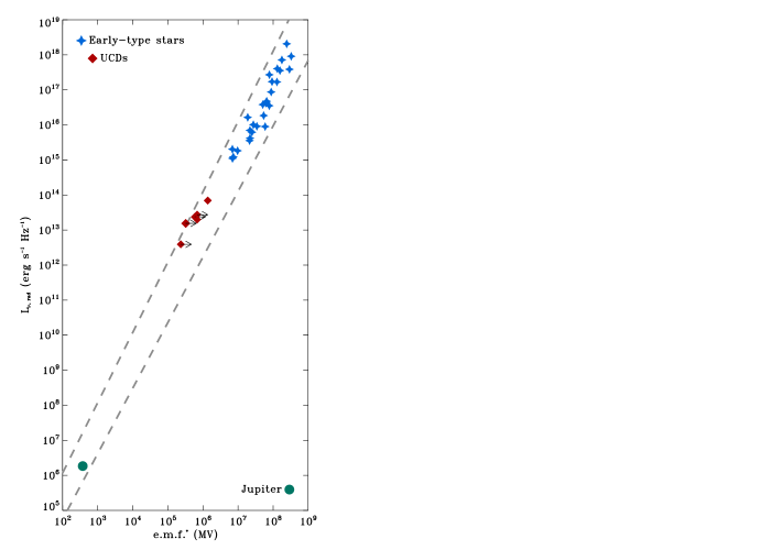
Figure 11: $L_{\nu,{\mathrm{rad}}}/{\mathrm{e.\,f.\,m.}^{\ast}}$ diagram. The dashed gray lines locate the boundary of the uncertainty range of the scaling relation derived by using the parameters of the early type magnetic stars only.

The UCDs are faint objects in the visual band. Further, those that are radio loud are also fast rotators (rotation periods of order an hour), allowing direct magnetic field measurements in only few cases. In some cases the magnetic fields of the UCDs can be indirectly constrained. In fact, following the basic theory of the ECM mechanism, the emission frequency ($\nu$) of the coherent pulses occurs close to local gyro-frequency. Since the gyro-frequency is related to the local magnetic field by the relation $\nu_{\mathrm{B}}=2.8\times B/{\mathrm{kG}}$ GHz, the polar field strength of the UCDs where the ECM is detected will be $B_{\mathrm{p}}\gtrapprox\nu/2.8$ kG. Hence, the lower limits of the polar field strengths reported in Table 3 were estimated from the maximum frequencies at which the coherent emission produced by the ECM was detected. In particular, the four listed UCDs showed coherent pulses at $\nu\approx 8.4$ GHz (Berger, 2002; Burgasser & Putman, 2005; Hallinan et al., 2007, 2008), thus $B_{\mathrm{p}}\gtrapprox 3$ kG.

To determine whether the radio behavior of UCDs matches the scaling relation given by Eq. 1 requires both reliable radio luminosities for the incoherent non-thermal radio emission and knowledge of stellar parameters, in particular the magnetic field strength, rotation period, and radius. For our analysis, we excluded UCDs that are members of binary systems. The incoherent fluxes reported in Appendix B have been used to estimate the radio luminosities of the six UCDs in Table 3. The few available radio measurements are mainly performed at a single frequency, particularly $\nu\approx 5$ or 8.4 GHz (see Appendix B).

The presence of stable electric fields within the large scale magnetospheres of the UCDs was proposed to have a possible role on the non-thermal electron production responsible for the radio emission (coherent and incoherent) from these objects (Doyle et al., 2010). In Fig. 11, the radio luminosities of the non-thermal incoherent emission of the small sample of UCDs analyzed here are reported as a function of their effective electromotive forces (or lower limits). Despite the limitations explained above, the UCD parameters lie in the $L_{\nu,{\mathrm{rad}}}/{\mathrm{e.\,f.\,m.}^{\ast}}$ diagram either within (or very close to) the uncertainty range extrapolated from the scaling relation established by the sample of early-type magnetic stars.

8 The scaling relationship for the radio emission applied to hot Jupiters

Hot Jupiters are giant gaseous planets orbiting very close to their parent stars. Due to the proximity to the star, hot Jupiters have suitable conditions to develop strong star planet magnetic interactions (SPMI), extending Bode’s law, that holds for the magnetized planets of the solar system, to the exo-planets (Zarka, 2007). Bode’s law is an empirical scaling relation between the power of the coherent auroral radio emission from a magnetized planet and the power dissipated when interacts with the magnetized plasma released by the parent star, and vice-versa. Due to their small orbits, the extrapolated Bode’s law predicts detectable coherent auroral radio emission from magnetized hot Jupiters (Zarka, 2007).

The auroral radio emission is tuned at the radio frequency typical of the ECM mechanism, that, as previously discussed (see Sec. 7.2), depends by the magnetic field strength of the body where it originates (star or planet). The estimated magnetic field strength of the exo-planets belonging to the hot Jupiter class ranges from few G (like the case of Jupiter) up to few hundred G (Yadav & Thorngren, 2017). Then, the expected ECM emission frequency lies in low frequency spectral domain (tens to a few hundred MHz). The tentative detection by the LOFAR interferometer of highly polarized low frequency radio emission from the hot Jupiter $\tau$ Bootes b has been recently reported (Turner et al., 2021). This result supports the Bode’s law extension beyond the Solar system, and further provides indirect evidence of magnetism occurring in exo-planets.

Table 4: Hot Jupiters parameters.

	$D$	$P_{\mathrm{rot}}$	$B^{(5)}$	$R^{(5)}$
Name	(pc)	(d)	(G)	(RJ)
HD 179949 b	$27.48(0.06)^{(1)}$	$\approx 7^{(3)}$	$\approx 90$	$1.22\pm 0.18$
HD 189733 b	$19.78(0.01)^{(1)}$	$1.7^{+2.9}_{-0.4}$(4)	$\approx 20$	$1.14\pm 0.03$
$\tau$ Bootes b	$15.62(0.05)^{(2)}$	$\approx 3.2^{(3)}$	$\approx 100$	$1.13\pm 0.17$
$\upsilon$ Andromedae b	$13.49(0.03)^{(2)}$	$\approx 12^{(3)}$	$\approx 80$	$1.25\pm 0.19$

• ⁽¹⁾Gaia Collaboration, 2018; ⁽²⁾van Leeuwen, 2007; ⁽³⁾Shkolnik et al., 2008; ⁽⁴⁾Brogi et al., 2016; ⁽⁵⁾Cauley et al., 2019.

The capability to detect low-frequency radio emission from the interaction of an exo-planetary magnetosphere with its parent star has been already discussed (Zarka, 2007). Similarly to the low-frequency radio emission, also the radio emission at the GHz frequency range, covered by the forthcoming Square Kilometre Array (SKA), has been already taken into account (Zarka et al., 2015). Exo-planetary auroral radio emission is a bright radio emission constrained to the low frequency spectral domain, however at the GHz radio frequencies the SPMI may provide detectable features too. Similarly to the auroral radio emission from Jupiter triggered by its moon Io, an exo-planet moving within the stellar magnetic field could be able to stimulate auroral radio emission on the magnetic flux tubes connected to the parent star. In this case the emission frequency of the auroral radio emission depends upon the stellar magnetic field. Magnetic field strengths at the kG level are common in case of late type stars (Reiners & Basri, 2007), then the auroral radio emission will be tuned at GHz radio frequencies. Such stellar auroral radio emission triggered by SPMI has been recently discovered from the star Proxima Cen (Pérez-Torres et al., 2021). As demonstrated by Zarka (2007), both types of SPMI produce auroral emission having radio power satisfying Bode’s law.

In accordance with the ECM elementary emission mechanism (Melrose & Dulk, 1982), auroral radio emission is a highly directive phenomenon, making it difficult to detect despite its strong emission level. Similarly to the incoherent non-thermal radio emission from Jupiter, magnetized hot Jupiters might also be direct sources of such isotropic emission tuned at GHz radio frequencies. The previous Secs. 7.1 and 7.2 support the prediction provided by the scaling relationship obtained by analyzing the behavior at the radio regime of the early-type magnetic stars and extrapolated to lower mass objects (UCDs and the planet Jupiter), for which the detection of their incoherent non-thermal radio emissions have been already reported. These results stimulated us to adopt the scaling relationship provided in this paper (Eq. 1) as a predictive tool for the incoherent radio emission from astrophysical objects surrounded by large scale magnetospheres and having known parameters. Among these, the hot Jupiter class is suitable. In fact, some of them are magnetized sub-stellar objects, whose magnetic field strength, radius, and rotation period have been constrained.

The favorable condition to produce incoherent non-thermal radio emission from a large-scale rotating magnetosphere is the corresponding strength of the magnetic field. In the cases of some hot Jupiters, that are particularly close to the Earth, the presence of magnetic field strengths higher than Jupiter’s have been reported (Cauley et al., 2019). The selected objects are listed in Table 4 with their corresponding parameters. The expected incoherent radio emission levels of the four magnetized hot Jupiters, derived using Eq. 1 with the corresponding parameter uncertainties, are reported in Fig. 12 as a function of the effective electromotive force generated by the rotation of these exo-planets. The expected fluxes are well below the $\mu$Jy level.

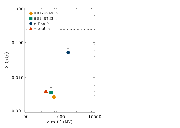
Figure 12: Expected fluxes at Earth of the four hot Jupiters analyzed. Fluxes calculated by extending the scaling relationship of the incoherent non-thermal radio emission of the early-type magnetic stars. The error-bars follow by the parameters uncertainty of the adopted scaling relationship (Eq. 1). The dotted line represent the SKA detection limit.

The most sensitive ground based radio interferometer operating at the GHz domain will be most likely the forthcoming SKA. In fact the detection limit of the SKA in its full operational state will be $\approx 0.24$ $\mu$Jy, for observations lasting $\approx 10$ minutes of integration time (Umana et al., 2015). As seen in Fig. 12, the expected fluxes of the four hot Jupiters are below the SKA detection limit. Probably, the hot Jupiters analyzed here do not rotate fast enough, or are not sufficiently magnetized to provide detectable incoherent radio emission. In any case, we suspect that in general it is unlikely to expect to detect the incoherent radio emission components of hot Jupiters. In fact, the star’s proximity, that is a suitable condition for triggering the low frequency auroral radio emission, makes it difficult to spatially resolve its incoherent non-thermal radio emission from the stellar radio emission.

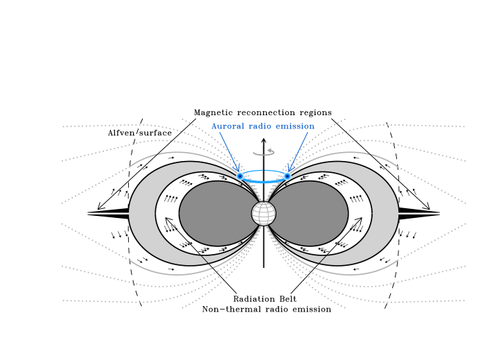
Figure 13: Schematic representation of the radio emission sites within a dipole-dominated magnetosphere of a typical early-type magnetic star. For this picture the field and rotation axes are assumed the same. The location of the radiation belt is highlighted by the white magnetic shell, with small arrows indicating the relativistic electrons. This region is the dominant source of the non-thermal stellar radio emission, and is located inside the inner magnetosphere. The cartoon is purely an idealization, the radiation belt and the Alvén surface are arbitrarily located. The Alfvén surface is far from the star (dashed line). Outside this surface the magnetic field lines are open (dotted lines). Magnetic reconnection events take place within the equatorial magneto-disk (dark region), with consequent production of fast-electrons, that, like the case of Jupiter, trigger the coherent and strongly beamed auroral radio emission (blue spots on the blue auroral ring).

The most favorable condition for non-thermal radio emission detection from giant exo-planets is the planetary orbital position far from their parent stars, making it possible to spatially resolve the radio emissions from both star and exo-planet. Further, the large distance strongly reduces the star-planet interaction effects, these ice giant exoplanets might be unable to produce detectable low frequency auroral radio emission, making the detection of the incoherent non-thermal radio emission the only way to search at the radio regime for exoplanets orbiting far from their parent stars. Non-thermal radio emission may be detectable by SKA in the case of ice giant exo-planets that, possibly, rotate faster than the tidally locked hot Jupiters and than produce higher strength magnetic fields, as expected from the rotation dependent dynamo efficiency. If the fluxes are above the detection threshold, the SKA angular resolution in its full operational state, $\approx 0.02$ arcsec at $\nu\approx 1$ GHz (Umana et al., 2015), or lower (depending by the observing frequency), could be able to easily resolve from their parent stars exo-planets orbiting at the same distance of Jupiter from the Sun and within 100 pc.

9 Discussion

The observed radio emission of early-type magnetic stars is compatible with gyro-synchrotron emission from a dipole-like magnetic shell co-rotating with the star. The radio spectral calculations allowed us to constrain the equatorial size ($L$ parameter) of the radiating magnetic shells (Sec. 3). Following the standard scenario for the radio emission from early B magnetic stars, the shell size was assumed to coincide with the equatorial Alfvén radius, which is the distance where the radiatively driven stellar wind opens the magnetic field lines.

The inferred wind mass-loss rates required to reproduce the radio spectra of the hottest stars are roughly close to (but always higher than) the theoretical expectations at the known effective stellar temperatures (Sec. 4.2). For the cooler stars, the above rough accordance totally fails (see Fig. 5). The surface chemical composition could play a role in estimation of the wind mass-loss rates (Krtička, 2014), or other mass-loss recipes (Vink et al., 2001) could be employed that predict higher values (see Shultz et al., 2019c for details). Ultimately, the expected mass loss is still lower than the value required for the radio modeling. Independent evidence for a mass-loss inconsistency at these spectral types comes from HST observations of the wind sensitive UV lines of the early A-type star HD 124224 (Krtička et al., 2019). Those data allow for only an upper limit to the wind mass loss, a limit that is discrepant with that required to explain the observed radio spectrum.

Reconciling the observed common behavior of the radio emission from the sample of early-type magnetic stars analyzed in this work, with the discordance between inferred and predicted mass-loss rates, indicates that we must abandon a physical relation between the Alfvén surface size at the equator ($R_{\mathrm{A}}$) to the size of the magnetic shell ($L$) radiating at the radio regime. Instead, the origin of the non-thermal radio emission must relate to a physical structure that is less dependent on stellar wind properties. We suggest that the non-thermal radio emission originates from radiation belts located inside the inner-magnetosphere of the early-type magnetic stars (see Fig. 13).

The stellar wind still plays an important role in this new picture. The wind is likely the primary source of ionized matter that fills the stellar magnetosphere. From a qualitative point of view, hot stars have favorable conditions for the onset of all the plasma processes that trigger the stellar radio emission, simply because their powerful winds quickly deposit a large quantity of ionized matter into their magnetospheres. Cooler stars are instead characterized by weak winds and consequently the plasma accumulation is slow.

The radiation belt located inside the inner magnetosphere may be at a significant distance from the current sheet regions, that form outside the equatorial Alfvén surface, and the site of magnetic reconnection events, which are the likely sources of electron acceleration. Now the question arises: what is the origin of the non-thermal electrons trapped within the radiation belt responsible for the observed radio emission? One explanation could be a relation between the origin of the relativistic electrons with the centrifugal breakout produced by the high-density magnetospheric plasma locked within the inner magnetosphere. The breakout mechanism has already been shown to explain plasma transport within the centrifugal magnetospheres of the B-type stars (Shultz et al., 2020; Owocki et al., 2020). This is also the case of Jupiter’s magnetosphere, where energetic electrons are produced in breakdown regions occurring between 15 and 30 $R_{\mathrm{J}}$ (Krupp et al., 2004). Jupiter’s radiation belt, located at $L<5$ $R_{\mathrm{J}}$, has a closed magnetic topology and is the planet’s source of the non-thermal radio emission. For the radio emission from Jupiter’s belt zone, the proposed source of non-thermal electrons is the radial diffusion from the farther Jovian magnetospheric regions, where these energetic electrons are likely produced (Bolton et al., 2004).

An alternative mechanism for the production of energetic electrons within closed magnetic field regions is the resonant interaction of the local plasma with low-frequency electromagnetic waves, known as whistler modes. It is this mechanism that seems dominant in the case of Earth’s radiation belt (Boyd et al., 2018), and also observed to be active within the radiation belts of the giant planets Jupiter and Saturn (Woodfield et al., 2014, 2019). To operate efficiently, the wave-particle resonant interactions require low densities, namely $\nu_{\mathrm{p}}\leq 2.5\nu_{\mathrm{B}}$ (Horne, Glauert & Thorne, 2003), where $\nu_{\mathrm{B}}$ is the gyro-frequency ($\nu_{\mathrm{B}}=2.8\times B/{\mathrm{G}}$ MHz) and $\nu_{\mathrm{p}}$ is the plasma frequency ($\nu_{\mathrm{p}}=9\times 10^{-3}\sqrt{N}_{\mathrm{e}}$ MHz). For the early-type stars of this paper, the typical strength of the magnetic field at distance $L$ is $B_{L}\approx 2$ G (Sec. 3.2), corresponding to a gyro-frequency $\nu_{\mathrm{B}}\approx 6$ MHz. It follows that the plasma density of the radiation belt compatible with local acceleration by wave-particle resonant interaction has to be lower than $2\times 10^{6}$ cm^-3.

The acceleration through this resonant interaction achieves its maximum efficiency for whistler modes at an oscillation frequency of $\nu\approx 0.35\nu_{\mathrm{B}}$ (Horne et al., 2003). The corresponding wave frequency of the resonant whistler mode will be $\nu\approx 2$ MHz, which is lower than the plasma frequency of the Earth’s ionosphere ($\lessapprox 10$ MHz). This puts strong technical limitations on observations below this low-frequency cutoff with ground-based radio telescopes (de Gasperin et al., 2018). But such low frequency radiation probably cannot be detected in any case, even if we observe outside the Earth’s ionosphere.

To reproduce the observed radio emission from the early-type magnetic stars, one must account for the presence of trapped thermal plasma located within the inner magnetosphere, with a density of order $10^{9}$ cm^-3 close to the stellar surface. Following the MCWS model, the density of trapped plasma decreases inversely with distance from the star. The plasma surrounding the radiation belt is expected to have a density of $\approx 10^{8}$ cm^-3. At this value, low-frequency electromagnetic waves cannot escape from the stellar magnetosphere. Consequently, wave-plasma interactions as a proposed electron acceleration mechanism cannot be directly verified. Furthermore, some process is needed for forming low-density cavities within the inner magnetosphere to allow the wave-plasma interaction to accelerate local electrons efficiently.

In the case of the Earth a correlation of whistlers mode with the electric discharges related to lightning (Green et al., 2005) was observed. The empirical correlation between the average radio luminosity of incoherent non-thermal radio emission and the magnetic flux rate (see Fig. 10) suggests that some kind of electrodynamic mechanism may act within the magnetospheres of the early-type magnetic stars. The electrodynamical processes acting within the rotating magnetosphere might be the engine to originate large scale currents and electric discharges. Like the case of the Earth, this might be a likely condition to originate low-frequency electromagnetic waves that, similarly to the magnetized planets of the solar system, might produce local plasma acceleration by resonant wave-particle interaction.

Following our new scenario of a radiation belt located within the inner-magnetosphere, there is a possible critical issue for the low-frequency coherent auroral radio emission stimulated by the ECM emission mechanism. Is this coherent emission capable of escaping from the inner-magnetosphere to be detectable? In fact, such stimulated radio emission originates from the deep magnetospheric regions close to the star. Hence, these low-frequency electromagnetic waves might be strongly suppressed by the gyro-resonant magnetic absorption of the thermal plasma surrounding the radiation belt, if the auroral radio emission arises from the same magnetic shell where the incoherent non-thermal radio emission originates.

The broad studies of Jupiter’s radio emission suggest a possible resolution to the issue raised above. Jupiter shows clear evidence of non-thermal radio emission from a radiation belt located close to the planet ($L<5$ R_J), and also various components of coherent radio emission. An important source of coherent emission is associated with the moon Io, but there is also a non-Io contribution arising from the magnetic field lines anchored at the planet’s surface at high latitudes, and coinciding with the main auroral oval. It was recognized that the footprints of these field lines are related to the magnetic field lines crossing the magnetic equatorial plane at a large distance ($L\gtrapprox 7$–15 R_J) and close to the breakdown regions where magnetic reconnection events have been identified. These reconnection events provide the injection of fast electrons that trigger on Jupiter the non-Io DAM (i.e. the component of the Jovian decametric radio emission (DAM) not related to the magnetic flux tube connected with the moon Io) and the bKOM (i.e. the Jovian broadband kilometric radiation) (Zarka, 1998, 2004). The Jupiter-like scenario was recently supported to be scalable also in the case of magnetic early type stars by the frequency dependent behavior of the wide band coherent emission from HD 124224 (CU Vir), the prototype of the class of early-type magnetic stars showing auroral radio emission, where several auroral radio emission components seems to be related to different magnetic field lines of the stellar magnetosphere (Das & Chandra, 2021).

Similar to Jupiter, the auroral radio emission of early-type magnetic stars might be triggered by the non-thermal electrons accelerated within the magnetospheric regions where the magnetic field strength is too weak to confine the magnetospheric wind plasma, or produced by continuous centrifugal breakouts events. The result is the formation of an equatorial magneto-disk site of magnetic reconnection. A cartoon that summarizes this scenario is given in Fig. 13. Even if this scenario is an over-simplified schematization of a true rotating stellar magnetosphere, this picture highlights that the injection of non-thermal electrons is not related to a unique acceleration site, where, possibly, different acceleration mechanisms are working. Beyond the magnetospheric regions where the wind plasma breaks the field lines, producing magnetic reconnection and consequent acceleration of electrons, energetic electrons can be also locally accelerated within the most internal regions where the magnetic field lines are closed, as seen in the case of Earth.

10 Conclusion and outlook

In this paper, we analyzed the incoherent gyro-synchrotron radio emission of a sample of early type magnetic stars, ranging from early-B to early-A type stars, as a function of their stellar parameters. As a result of our study, we report the existence of a strict correlation between the non-thermal radio luminosity ($L_{\nu,\mathrm{rad}}$) and the ratio of magnetic flux to the rotation period ($\Phi/P_{\mathrm{rot}}$), given by the Eq. 1 and shown in Fig. 10. This relationship appears to be something analogous to the scaling relationship that describes the coherent auroral radio emission of the magnetized body of the Solar system, formalized by the radio-magnetic Bode’s law and which is extrapolated up to the exo-planets (Zarka, 2007).

We also reviewed the wind scenario used to account for the non-thermal radio emission of these stars. The stellar wind has still a key role to supply ionized material within the magnetospheres of the early-type magnetic stars. But, unlike what was previously assumed, we found that the equatorial size of the magnetospheric region radiating incoherent gyro-synchrotron radio emission is not large enough to intercept the regions in which the wind pressure equals the magnetic tension. To explain the features of the non-thermal radio emission from such hot magnetized stars we proposed the existence of a Jupiter-like radiation belt within the magnetospheres of the early-type magnetic stars. The existence of a radiation belt around the magnetized planets of the Solar system is a well-known phenomenon, already taken into account in stellar cases too. To explain the origin of the incoherent non-thermal radio emission from UCDs, a plasma radiation belt has been proposed to exist within their magnetospheres (Hallinan et al., 2006). This idea applied in the context of the early type magnetic stars leads to convenient results. In fact, in this new picture, the magnetic shell where the non-thermal radio emission originates is formally decoupled from the wind mass loss rate strength. Following this new wind paradigm, a more complex picture seems to come out with regard to the origin of the non-thermal electrons responsible for the incoherent gyro-synchrotron emission. In particular, the current sheets produced by the wind magnetic breakout can not provide unique (and primary) acceleration sites.

Importantly, the scaling relationship between $L_{\nu,\mathrm{rad}}$ and $\Phi/P_{\mathrm{rot}}$ for the early-type magnetic stars, also successfully predicts the non-thermal radio emission from some (six) UCDs and the planet Jupiter. The parameter $\Phi/P_{\mathrm{rot}}$ is related to the effective electromotive force generated by the rotation of a large-scale and well-ordered magnetic field. The rotation stimulates electrodynamic processes occurring within the stellar magnetosphere, that appear key to establishing the radio emission level of the dipole like magnetospheres surrounding objects at both the top and at the bottom of the main sequence (see Fig. 11). It is then possible that the mechanism for acceleration of non-thermal electrons may be related to large-scale stationary current systems.

The various plasma configurations that we have suggested as possibly existing within the magnetospheres of early-type stars certainly demands further investigation. And while we have identified a scaling relation that span magnetospheres from early-type massive stars to UCDs and planets, this needs further study. The early-type magnetic stars have a favorable condition to fill their magnetospheres with ionized material. In fact, the stellar wind, even if in some cases the mass-loss rate is at a very weak level, has a key role as a plasma source. The UCDs and Jupiter have well-ordered dipolar fields, but are cold objects lacking winds of any significance, yet they produce non-thermal radio emission. However, if some other plasma source fills their magnetospheres (i.e. exo-planetary volcanic activity analogous to that of the moon Io), suitable conditions for the radio emission generation will be realized. The radio luminosity of incoherent emission from UCDs is low, and for only a few such emission has been detected, while simultaneously having reliable magnetic field strengths. Nonetheless, the few cold objects that we have analyzed display radio behavior in remarkable accord with the empirical scaling relationship deduced from the early-type stars. This is a clear hint of a common behavior among both stars and substellar objects surrounded by large-scale and stable magnetospheres, suggesting that an underlying and unifying physical mechanism is at work. In particular, it is plausible to hypothesize the existence of a common acceleration mechanism of electrons to relativistic energies operating within the magnetospheres among these extremely different classes of objects.

Future work must enlarge the sample of early-type magnetic stars to refine the empirical relationship for the non-thermal radio emission from ordered magnetospheres. In particular, a systematic search for radio emission at the top of the main sequence should be useful for the indirect estimation of stellar parameters, in particular the stellar magnetic field strength. In fact, on the basis of the empirical dependence between radio luminosity and stellar parameters, the detection of non-thermal radio emission might be used to constrain the stellar magnetic field strength.

The next generation of ground based radio interferometer (e.g. SKA) will quickly be able to reach a detection limit at the $\mu$Jy level, such that brighter early-type magnetic stars ($L_{\nu,{\mathrm{rad}}}\approx 10^{18}$ ergs s^-1 Hz^-1) located close to the Galactic center ($\approx 9$ kpc distance) will be easily detected (expected flux levels $\approx 10$ $\mu$Jy). Ap/Bp stars are uniformly distributed in space (Renson & Manfroid, 2009), and the number recognized as magnetic stars is rapidly increasing (Fossati et al., 2015; Wade et al., 2016). At the present, spectropolarimetric measurements are able to perform reliable measurements of stellar magnetic fields only for stars located within 1–2 kpc from the Sun (Shultz et al., 2019a; Bagnulo et al., 2020). We emphasize that radio emission could be used as another diagnostic tool for stellar magnetism, and leveraged to investigate the incidence of magnetism at the top of the main sequence. The origin of magnetic fields of early-type stars, and their persistence over their MS life, and beyond (Neiner et al., 2017; Martin et al., 2018), is a crucial matter. In fact, the magnetic field of the very massive stellar progenitor might be significant to the core-collapse supernovae explosion and the potential birth of magnetars (Bucciantini et al., 2009; Kasen & Bildsten, 2010).

Data availability

The data underlying this article are available in the article and in its appendices.

Appendix A Radio measurements of the individual early type stars

A.1 HD 12447

This magnetic Ap star was detected at 1.4 GHz by the FIRST (Faint Images of the Radio Sky at Twenty centimeters) survey performed by the VLA (Becker, White & Helfand, 1995), the flux is $S=0.7\pm 0.1$ mJy (Helfand, White & Becker, 2015). The stellar radio emission was also detected at 3.6 cm (corresponding to $\approx 8.4$ GHz) with a flux level of $S=0.37\pm 0.09$ mJy (Drake, Wade & Linsky, 2006). Further, HD 12447 holds in the tile T11t04 observed at 3 GHz in two epoch of the VLA Sky Survey (VLASS1.1 and 2.1) and was also detected at both epochs with similar flux level, on average $0.69\pm 0.09$ mJy. The radio luminosity of HD 12447 reported in Table 1 has been obtained using the average fluxes at these available radio frequencies. Mean frequency $<\nu>\approx 3.3$ GHz.

A.2 HD 19832

HD 19832 was detected by the VLA at $8.4$ GHz, $S=0.45\pm 0.12$ mJy (Drake et al., 2006), and at 3 GHz by the second half of the first epoch (VLASS1.2, tile T17t05) of the VLASS ($S=0.5\pm 0.1$ mJy). Also in this case, the radio luminosity reported in Table 1 has been retrieved by the average flux of the two radio measurements, at the corresponding mean frequency $<\nu>\approx 5$ GHz.

A.3 HD 27309

Measurements of the radio emission of HD 27309 are available at three distinct frequencies, respectively at $\nu=3$ GHz (VLASS1.2, tile T16t06), $S=0.4\pm 0.1$ mJy, and at 5, $S=0.38\pm 0.02$ mJy, and 8.4 GHz, $S=0.33\pm 0.02$ mJy (Drake et al., 2006). To estimate the radio luminosity of HD 27309 (Table 1), the average flux has been used. Mean frequency $<\nu>\approx 5$ GHz.

A.4 HD 34452

The detection of the radio emission of IQ Aur (HD 34452) at $\nu=5$ GHz ($S=0.48\pm 0.09$ mJy) was firstly reported by Drake et al. (1987) and then confirmed by Linsky et al. (1992) ($S=0.32\pm 0.05$ mJy). The average flux has been used to estimate the radio luminosity of HD 34452.

A.5 HD 35298

It was recently discovered by Das et al. (2019b) that HD 35298 is a source of low frequency ($\nu\leq 1.4$ GHz) high strength (flux level approaching up to $\approx 10$ mJy) coherent auroral radio emission. Such maser emission is constrained within a well defined range of phases and is superimposed above the basal emission produced by the incoherent gyro synchrotron mechanism. The incoherent component of the HD 35298 emission was firstly measured at 5 GHz by Linsky et al. (1992) ($S=0.28\pm 0.06$ mJy). Measurements at other frequencies are also available in the literature ($S=0.29\pm 0.07$ mJy at $\nu=8.4$ GHz; Drake et al., 2006). Further, our unpublished high frequencies VLA observations (project code: AL618) allowed us to measure the fluxes of HD 35298 at $\nu=15$ GHz ($S=0.32\pm 0.03$ mJy) and at $\nu=22$ GHz ($S=0.13\pm 0.02$ mJy). These radio measurements cover a wide frequency range and have been averaged to estimate the luminosity reported in Table 1 at the mean frequency $<\nu>\approx 10.9$ GHz.

A.6 HD 35502

HD 35502 holds in the tile T10t09 observed over two epochs of the VLA Sky Survey at 3 GHz (VLASS1.1 and 2.1), with fluxes $S=2.6\pm 0.1$ and $S=3.0\pm 0.1$ mJy. Further, unpublished multi-wavelengths VLA radio observations of HD 35502 have been retrieved querying the NRAO data archive (project code: AL388). This data set has been processed by us to obtain the following radio measurements: $S=1.7\pm 0.1$ mJy at $\nu=5$ GHz; $S=2.28\pm 0.07$ mJy at $\nu=8.4$ GHz; $S=1.36\pm 0.06$ mJy at $\nu=15$ GHz. Another measurement performed at 8.4 GHz is reported in the literature. The flux of HD 35502 at that observing epoch was $S=2.97\pm 0.1$ mJy (Drake et al., 2006). These multi-frequencies measurements are used to obtain the average radio luminosity listed in Table 1. Mean frequency $<\nu>\approx 6.6$ GHz.

A.7 HD 36485

Table 5: HD 36485 radio spectrum.

$\nu$	$<S_{\nu}>$
(GHz)	(mJy)	notes
$0.61^{\ast}$	$0.6\pm 0.2$	Chandra et al. (2015)
$1.4$	$0.8\pm 0.2$	Chandra et al. (2015); AL267†
$3^{\ast}$	$1.4\pm 0.2$	VLASS1.1 and 2.1 (tile T10t09)
$5$	$1.1\pm 0.2$	Leone et al. (2010)
$8.4$	$1.0\pm 0.2$	AL267†; AL388
$15$	$0.8\pm 0.2$	AL267†; AL388

• ^∗ Less than three measurements. ^† NRAO image archive.

The radio emission of HD 36485 was firstly reported by Drake et al. (1987). HD 36485 was observed many times at $\nu=5$ GHz. These radio observations cover the whole stellar rotation period. The light curve at 5 GHz was performed by Leone et al. (2010) and shows a moderate rotational modulation. Additional radio observations of HD 36485, performed by the VLA at other frequencies, exists. In this paper, we analyzed all the available data set. The VLA project AL267, beyond the already published 5 GHz radio measurements, contains observations performed at $\nu=1.4$, 8.4 and 15 GHz, performed at three different epochs (1992-Oct-11, 13, and 15). These multi-frequency observations have been processed by the standard VLA pipeline. The radio maps are available querying the NRAO Image Retrieval Tool and are used for measuring the stellar radio fluxes. Further unpublished VLA observations at 8.4 and 15 GHz are available (project AL388). These archival data have been reduced by us using the standard calibration procedure enabled in casa. Ancillary radio measurements at 0.61 and 1.4 GHz are also collected (Chandra et al., 2015). Finally, HD 36485 was also detected at 3 GHz by the two epochs of the first half VLASS (VLASS1.1 and 2.1). All the available radio measurements performed at the same frequency have been averaged, listed in Table 5, and shown in Fig. 2. In the case of more than one measurement at the same frequency, the uncertainty has been estimated adding in quadrature the measurements dispersion and the average of the individual errors. The data in Table 5 has been averaged to estimate the stellar radio luminosity at the mean frequency $<\nu>\approx 3.4$ GHz.

A.8 HD 37017

Table 6: HD 37017 radio spectrum.

$\nu$	$<S_{\nu}>$
(GHz)	(mJy)	notes
$0.61^{\ast}$	$0.6\pm 0.3$	(a)
$1.4$	$1.6\pm 0.5$	(a); (b); (c)
$3^{\ast}$	$1.7\pm 0.7$	VLASS1.1 and 2.1 (tile T09t09)
$4.5$	$2.0\pm 0.2$	(d)
$5$	$2.0\pm 0.5$	(b); (e); (f)
$8.4$	$2.1\pm 0.3$	AL267†; AL388
$15$	$1.8\pm 0.4$	(b); (c); AL267†; AL388; AL618
$22$	$2.0\pm 0.9$	(c); AL234†; AU53†; AL618
$43^{\ast}$	$1.9\pm 0.1$	AL618

• ^∗ Less than three measurements. ^† NRAO image archive. (a) Chandra et al., 2015; (b) Drake et al., 1987; (c) Leone, Umana & Trigilio, 1996; (d) Kounkel et al., 2014. (e) Leone & Umana, 1993; (f) Trigilio et al., 2004.

The radio emission of HD 37017 was firstly measured by Drake et al. (1987) and then the rotation modulation effect on the 5 GHz stellar radio emission was analyzed (Leone, 1991; Leone & Umana, 1993). The 5 GHz light curve of HD 37017 was calculated by Trigilio et al. (2004) and compared with the available measurements covering the stellar rotation period. The average value of these measurements is listed in Table 6. A reliable VLA detection ($\nu=4.5$ GHz) has been also reported by Kounkel et al. (2014) The tentative detection of the low-frequency ($\nu=610$ MHz) emission of HD 37017 was reported by Chandra et al. (2015), further, measurements at other radio frequencies are also reported in the literature. The ancillary data complemented by unpublished measurements (reduced by us or processed by the standard VLA pipeline) acquired at the same frequency are averaged altogether. Further, HD 37017 was detected at 3 GHz by the VLASS (in the table the average of the two epochs of the first half sky survey, respectively VLASS1.1 and VLASS2.1, was reported). The average spectrum reported in Table 6 is pictured in Fig. 2. The mean flux value has been used to estimate the radio luminosity of HD 37017. Mean frequency $<\nu>\approx 5.8$ GHz.

A.9 HD 37479

The non-thermal radio emission of HD 37479 was firstly measured by Drake et al. (1987). This star has been then subject of many radio observations. A detailed study of the multi-frequency radio emission of HD 37479 was performed by Leto et al. (2012), where a great number of radio measurements are reported. The radio survey of the Orion region performed by the VLA at 4.5 and 7.5 GHz (Kounkel et al., 2014) also detected the radio emission of HD 37479. Chandra et al. (2015) explored the HD 37479 behavior at the low frequency spectral region ($\nu=610$ MHz). HD 37479 was also detected at 3 GHz by the VLASS in two epochs (1.1 and 2.1). The data available at each radio frequency have been averaged, this average radio spectrum is reported in Table 7 and pictured in Fig. 2. The reported errors are the sum in quadrature of the dispersions of the data acquired at the same frequency and of the average of the uncertainties of the individual measurements. The mean value of these multi-frequencies radio measurements has been used to estimate the radio luminosity at the mean frequency $<\nu>\approx 5.9$ GHz.

A.10 HD 40312

Two distinct detections with similar fluxes of the stellar radio emission at 5 GHz exist (Linsky et al., 1992). It was commonly observed the rotational modulation of the radio emission from the hot magnetic stars. To take into account the expected radio variability, we assumed the uncertainty of 50%. The measured flux ($S\approx 0.3$ mJy) has been used to estimate the radio luminosity of HD 40312.

Table 7: HD 37479 radio spectrum.

$\nu$	$<S_{\nu}>$
(GHz)	(mJy)	notes
$0.61^{\ast}$	$1.2\pm 0.3$	(a)
$1.4$	$2.3\pm 0.5$	(a); (b); (c)
$3^{\ast}$	$3.0\pm 0.2$	VLASS1.1 and 2.1 (tile T10t09)
$4.5$	$3.7\pm 0.1$	(d)
$5$	$3.8\pm 0.5$	(c)
$7.5$	$3.8\pm 0.2$	(d)
$8.4$	$3.8\pm 0.6$	(c)
$15$	$4.0\pm 0.9$	(c)
$22$	$3.7\pm 0.9$	(c)
$43$	$3.1\pm 0.9$	(c)

• ^∗ Less than three measurements. (a) Chandra et al., 2015; (b) Linsky et al., 1992; (c) Leto et al., 2012; (d) Kounkel et al., 2014.

A.11 HD 79158

Only one detection of the radio emission from HD 79158 exists. This star was observed at 8.4 GHz and detected with the flux of $S=0.45$ mJy (Drake et al., 2006). To take into account possible rotational modulation, we assumed a flux uncertainty of 50%. This single data has been used to estimate the radio luminosity of HD 79158.

A.12 HD 112413

This is the prototype of the class of variable stars of $\alpha^{2}$ CVn type. HD 112413 ($\alpha^{2}$ CVn) was detected at 1.4 GHz by the FIRST survey ($S=0.77\pm 0.09$ mJy; Becker et al., 1995). This star was also detected at 8.4 GHz ($S=0.29$ mJy; Drake et al., 2006) and at 3 GHz by the VLASS. The source was detected by both epochs of the first half sky survey (VLASS1.1 and 2.1, tile T20t17), the average flux is $S=1.2\pm 0.2$ mJy. These multi-frequency detections have been averaged to estimate the radio luminosity of HD 112413 (Table 1). Mean frequency $<\nu>\approx 3.3$ GHz.

A.13 HD 118022

HD 118022 is the first star, which is not the Sun, in which the effect of the magnetic field was revealed in the stellar spectra (Babcock, 1947). Its radio emission was detected by the second epoch of the VLA Sky Survey (VLASS1.2), tile T11t21, the measured flux is $S=0.5$ mJy. This star was already observed by the VLA in the early 1990s at 8.4 GHz (project AD288), but the poor quality image prevents us from detecting its radio emission. Also in this case, it was assumed the flux uncertainty of 50% to estimate the radio luminosity of HD 118022.

A.14 HD 124224

Table 8: HD 124224 radio spectrum.

$\nu$	$<S_{\nu}>$
(GHz)	(mJy)	notes
$1.4$	$2.5\pm 0.6$	(a); (b); (c); (d)
$2.5$	$3.2\pm 0.4$	(c)
$3^{\ast}$	$2.7\pm 0.2$	VLASS1.2 (tile T11t22)
$5$	$3.9\pm 0.6$	(e)
$8.4$	$3.9\pm 0.6$	(e)
$15$	$3.4\pm 0.6$	(e)
$22^{\ast}$	$3\pm 1$	(a); AL618
$87.7^{\ast}$	$1.3\pm 0.3$	(e)

• ^∗ Less than three measurements. (a) Leone et al., 1996; (b) Trigilio et al., 2000; (c) Trigilio et al., 2008; (d) Helfand et al., 2015; (e) Leto et al., 2006; (f) Leone et al., 2004.

This is the first star where the coherent auroral radio emission was observed (Trigilio et al., 2000) and is widely studied at the radio regime (Leto et al., 2006). In this paper we collected many already published multi frequency radio measurements. Further, we analyzed our unpublished high-frequency VLA observations (project code AL618), data analyzed and imaged using casa. The radio measurements performed at the same radio observing band were averaged altogether, the related flux uncertainty is the sum in quadrature of the measure dispersion and the mean value of the individual errors. The average spectrum of HD 124224 is pictured in Fig. 2. The mean value of the data listed in Table 8 has been used to estimate the radio luminosity of HD 124224. Mean frequency $<\nu>\approx 7.7$ GHz.

A.15 HD 133652

One epoch VLA observation at 8.4 GHz of HD 133652 exists. A tentative detection of the stellar radio emission ($S=0.24$ mJy) is reported by Drake et al. (2006). Also in this case we adopted the flux uncertainty of 50% to estimate the radio luminosity of HD 133652.

A.16 HD 133880

HD 133880 was firstly observed by the ATCA interferometer covering the whole stellar rotation period (Lim, Drake & Linsky, 1996). The above data set allowed to perform the light curves at 5 and 8.4 GHz (Bailey et al., 2012). At lower radio frequencies HD 133880 evidenced enhanced emission constrained in a narrow range of phases (Chandra et al., 2015), later explained as coherent auroral radio emission (Das et al., 2018). Further, the wide band analysis of the auroral emission from HD 133880 allowed to evidence the longitudinal dependence of the plasma accumulation within the stellar magnetosphere (Das, Chandra & Wade, 2020). Despite its low sky latitude ($\delta=-40.5839^{\circ}$) this star is visible also by the VLA. The archival data set AD348 contains observations performed at three different epochs (1995-Feb-15, 16, and 17), the images are available querying the NRAO image archive. Further, HD 133880 was detected also at 43 GHz (VLA data set AL388 reduced and imaged in this paper). The low frequencies measurements ($\nu=0.61$ and 1.4 GHz; Chandra et al., 2015) acquired at phases where the auroral radio emission of HD 133880 is not observable have been used to estimate the incoherent emission component. Also in the case of measurements at the higher frequencies, the data at the same frequency have been averaged. The mean radio spectrum is reported in Table 9 and pictured in Fig. 2. The average flux of HD 133880 performed using all the available frequencies has been used to estimate its radio luminosity at the mean frequency $<\nu>\approx 5.3$ GHz.

Table 9: HD 133880 radio spectrum.

$\nu$	$<S_{\nu}>$
(GHz)	(mJy)	notes
0.61	$2.2\pm 0.7$	Chandra et al. (2015)
$1.4$	$3\pm 1$	Chandra et al. (2015)
$5$	$3.5\pm 0.8$	Bailey et al. (2012)
$8.4$	$3.6\pm 0.6$	Bailey et al. (2012)
$15$	$3.2\pm 0.5$	AD348†
$43^{\ast}$	$1.0\pm 0.2$	AL388

• ^∗ Less than three measurements. ^† NRAO image archive.

A.17 HD 142184

Table 10: HD 142184 radio spectrum.

$\nu$	$<S_{\nu}>$
(GHz)	(mJy)	notes
$0.8875^{\ast}$	$6.2\pm 0.2$	Pritchard et al. (2021)
$1.4^{\ast}$	$12.6\pm 0.6$	Condon et al. (1998)
$3^{\ast}$	$30\pm 2$	average of VLASS1.1 and 2.1 (tile T05t24)
$6$	$73\pm 15$	Murphy et al. (2010) ; Leto et al. (2018)
$8^{\ast}$	$95\pm 5$	Murphy et al. (2010)
$10$	$100\pm 20$	Leto et al. (2018)
$15$	$110\pm 20$	Leto et al. (2018)
$20^{\ast}$	$104\pm 6$	Murphy et al. (2010)
$22$	$120\pm 30$	Leto et al. (2018)
$33$	$130\pm 30$	Leto et al. (2018)
$44$	$120\pm 40$	Petrov et al. (2012); Leto et al. (2018)
$102^{\ast}$	$115\pm 20$	Leto et al. (2018)
$292^{\ast}$	$32.5\pm 3$	Leto et al. (2018)

• ^∗ Less than three measurements.

HD 142184 is a bright radio source detected up to the millimeter range, in fact, it was detected by the ALMA telescope (Leto et al., 2018). The measurement at the lowest available frequency ($\nu=887.5$ MHz) has been performed by the Australian SKA Pathfinder (ASKAP) interferometer (Pritchard et al., 2021). Almost all the available radio measurements of this magnetic star have been here collected. The fluxes acquired at similar observing frequencies have been averaged, these are listed in Table 10. At the lower frequencies the spectral dependence of the polarization fraction of the incoherent emission from HD 142184 evidenced a decaying trend, the polarization fraction decreases from a level of $\approx 10$ % at 44 GHz down to a few % at 6 GHz (Leto et al., 2018), this is in accordance with the canonical incoherent gyro-synchrotron emission mechanism. The low frequency ASKAP data ($\nu=887.5$ MHz) presents a circular polarization fraction of $\approx 22$%. This high level of circular polarization fraction observed at $887.5$ MHz is incompatible with the canonical spectral dependence of the circularly polarized emission from the incoherent gyro-synchrotron mechanism, this is a highly plausible hint that also the coherent auroral radio emission contributes to the low frequency radio emission from HD 142184. Then, the flux at $\nu=0.8875$ GHz listed in Table 10 is the total intensity given by Pritchard et al. (2021) reduced of the 22%, assumed as the auroral coherent emission fraction contaminating the incoherent non-thermal emission at $\nu=0.8875$ GHz. The mean spectrum is pictured in Fig. 2. The average radio luminosity of HD 142184, at the mean frequency $<\nu>\approx 13.5$ GHz, is reported in Table 1.

A.18 HD 142301

Table 11: HD 142301 radio spectrum.

$\nu$	$<S_{\nu}>$
(GHz)	(mJy)	notes
$1.5$	$2.8\pm 0.4$	Leto et al. (2019)
$3^{\ast}$	$2.6\pm 0.2$	VLASS1.2 (tile T04t24)
$5$	$4.0\pm 0.7$	Leto et al. (2019)
$8.4$	$3.8\pm 0.9$	Linsky et al. (1992); AL388
$15^{\ast}$	$3.4\pm 0.5$	Leone et al. (1996); AL388
$43^{\ast}$	$2.9\pm 0.2$	AL388

• ^∗ Less than three measurements.

Multifrequency measurements of the incoherent non-thermal radio emission of HD 142301 are reported by Linsky et al. (1992) and by Leone et al. (1996). HD 142301 is also a source of strongly polarized coherent auroral radio emission (Leto et al., 2019). Such kind of maser emission is constrained to a narrow range of the stellar rotational phases. To estimate the incoherent contribution alone, we average the 1.5 and the 5 GHz measurements acquired at phases far from the coherent pulses. Further, HD 142301 was detected by the VLASS at 3 GHz and unpublished VLA observations (project AL388) also revealed the high frequency contribution of the incoherent stellar radio emission (data set reduced and analyzed in this paper). The radio measurements acquired at the same frequency range have been averaged, the average spectrum is reported in Table 11 and shown in Fig. 2. The mean flux is used to estimate the stellar radio luminosity at the mean frequency $<\nu>\approx 7$ GHz.

A.19 HD 142990

The confirmed evidence of coherent auroral radio emission from HD 142990 was reported by Das et al. (2019a), which observed this star at low frequency ($\nu\approx 600$ MHz and $\nu\approx 1.4$ GHz) using the GMRT. At these low frequencies, the auroral emission from HD 142990 was observed in form of strongly polarized large pulses, that strongly contaminate the basal incoherent emission component. This condition make unreliable the estimation of the low-frequency incoherent emission component, that was roughly estimated at the mJy level. The incoherent emission component of HD 142990 was instead clearly measured at higher frequency bands. The average flux of HD 142990 measured at 5 GHz by Linsky et al. (1992), by Leone et al. (1994), and by us, analyzing archival VLA data (project AL388), is $S=1.9\pm 0.3$ mJy. A similar flux level was observed at 8.4 GHz ($S=1.8\pm 0.3$ mJy; Linsky et al., 1992 and VLA project AL388). The mean flux between the 5 and 8.4 GHz measurements has been used to estimate the stellar radio luminosity. Mean frequency $<\nu>\approx 6.5$ GHz.

A.20 HD 144334

The radio emission of HD 144334 at $\nu=5$ GHz was detected in two different epochs by Linsky et al. (1992). The average flux is $S=0.3\pm 0.15$ mJy, the uncertainty is obtained adding in quadrature the measurements dispersion and the average of the individual errors. The above flux was used to estimate the radio luminosity.

A.21 HD 145501

Multifrequency radio measurements ($\nu=1.4$, 5, and 8.4 GHz) of HD 145501 were reported by Linsky et al. (1992). The detection at 5 GHz was confirmed by Leone et al. (1994). This star has been also detected at 3 GHz ($S=1.45\pm 0.2$ mJy) by the VLASS (VLASS1.2 tile T06t25). The measured fluxes levels are almost comparable within the explored frequency range, the corresponding average flux is $1.6\pm 0.3$ mJy, which was used to estimate the luminosity of HD 145501 at the mean frequency $<\nu>\approx 3.6$ GHz.

A.22 HD 147932

Table 12: HD 147932 radio spectrum.

$\nu$	$<S_{\nu}>$
(GHz)	(mJy)	notes
$1.6$	$9\pm 4.5$	this paper
$2.6$	$15\pm 4$	this paper
$5.5$	$20\pm 4$	this paper
$9$	$21\pm 4$	this paper
$16.7^{\ast}$	$20.7\pm 0.2$	Leto et al. (2020b)

• ^∗ Flux from the total map (see Leto et al., 2020b).

Among the hot magnetic stars already known as sources of coherent auroral radio emission (ARE), at the present time, HD 147932 shows the unique behavior to have the auroral radio emission always detectable. This star does not evidence any preferred phase where the low frequency highly polarized coherent pulses were detected (Leto et al., 2020b). In fact, its peculiar geometry makes always visible the highly beamed maser emission responsible for the ARE. To disentangle the components arising from the two emission mechanisms, incoherent (gyro-synchrotron emission) and coherent (cyclotron maser), as a first approximation, we assume all the circularly polarized flux produced by the ARE. Hence, the subtraction of the average polarized flux (ATCA data available in Leto et al., 2020b) from the average total intensity supplies a reliable estimation of the incoherent radio spectrum of HD 147932. The fluxes, estimated at each observing frequency with the corresponding error propagation, are listed in Table 12. HD 147932 was also observed by the VLA, source detected at 1.4 GHz by the NVSS ($S=9.4\pm 0.6$ mJy; Condon et al., 1998) and by the project AK460 (NRAO image archive, $S\approx 18$ mJy), and at 3 GHz, VLASS1.2 (tile T05t25) $S\approx 12$ mJy, but the fraction of their polarized emission is unavailable. Therefore, considering the peculiar behavior of HD 147932, these VLA data have not been used. The radio spectrum of the gyro-synchrotron emission component is shown in Fig. 2, the corresponding average flux has been used to estimate the stellar radio luminosity at the mean frequency $<\nu>\approx 5.1$ GHz.

A.23 HD 147933

Table 13: HD 147933 radio spectrum.

$\nu$	$<S_{\nu}>$
(GHz)	(mJy)	notes
$1.6$	$5.5\pm 2$	this paper; NVSS; AK460†
$2.6$	$7\pm 2$	this paper; VLASS1.2 (tile T05t25)
$5.5$	$7\pm 2$	Leto et al. (2020a)
$9$	$8\pm 2$	Leto et al. (2020a)
$16.7$	$8\pm 2$	Leto et al. (2020a)
$21.2$	$7.5\pm 2$	Leto et al. (2020a)

• ^† NRAO image archive.

The behavior at the radio regime of HD 147933 has been recently studied using multi-epoch and multifrequency ATCA observations (Leto et al., 2020a). This star show coherent low frequency pulses superimposed to the basal incoherent non-thermal emission. The ATCA observations were performed using wide band backends (bandpass 2 GHz wide at each observing frequency). To better analyze the low frequency spectral dependence of the stellar radio emission, in this paper, we reanalyzed the L-band ATCA measurements of HD 147933. This dataset has been split in two sub-bands, 1 GHz wide, centered at 1.6 and 2.6 GHz. The low frequency pulses were observed at narrow phases intervals, which were excluded from the data average. The radio emission of HD 147933 was also detected by the VLA at 1.4 GHz, by the NVSS ($S=10.8\pm 0.6$ mJy; Condon et al., 1998) and unpublished archival data (project AK460: $S=8.9\pm 0.3$ mJy), and at 3 GHz (VLASS: $S=7.7\pm 0.2$ mJy). The VLA measurements have been averaged with the ATCA data at the closest frequency. The average radio spectrum of HD 147933 is listed in Table 13 and pictured in Fig. 2. The average of these spectral measurements has been used to estimate the radio luminosity reported in Table 1 at the mean frequency $<\nu>\approx 6.5$ GHz.

A.24 HD 170000

The radio emission of this magnetic star was detected at 8.4 GHz ($S=0.45$ mJy; Drake et al., 2006). HD 170000 has been also detected by the VLASS at 3 GHz (VLASS1.1 and 2.1, tile=T28t10; fluxes respectively: $S=0.5\pm 0.1$ and $S=0.8\pm 0.1$ mJy). These radio measurements have been averaged to estimate the radio luminosity of HD 170000. Mean frequency $<\nu>\approx 5$ GHz.

A.25 HD 175362

This star was detected at 5 GHz by Linsky et al. (1992) in two distinct epochs. The average flux ($S=0.32\pm 0.1$ mJy, uncertainty estimated adding in quadrature the data dispersion and the average map noise) is used to calculate the radio luminosity of HD 175362.

A.26 HD 176582

HD 175582 was detected at 8.4 GHz ($S=0.46$; Drake et al., 2006). Further, stellar radio emission was tentatively detected at 3 GHz (VLASS1.1, tile=T20t24, $S\approx 0.3$ mJy). To estimate the radio luminosity of this star we used the average flux $S=0.4\pm 0.1$ mJy, at the mean frequency $<\nu>\approx 5$ GHz.

A.27 HD 182180

Table 14: HD 182180 radio spectrum.

$\nu$	$<S_{\nu}>$
(GHz)	(mJy)	notes
$1.4^{\ast}$	$7.9\pm 0.6$	Condon et al. (1998)
$3^{\ast}$	$11.3\pm 0.2$	VLASS1.1 (tile T04t30)
$6$	$16\pm 3$	Leto et al. (2017a)
$10$	$17\pm 4$	Leto et al. (2017a)
$15$	$16\pm 3$	Leto et al. (2017a)
$22$	$16\pm 3$	Leto et al. (2017a)
$33$	$15\pm 3$	Leto et al. (2017a)
$44$	$13\pm 2$	Leto et al. (2017a)

• ^∗ Less than three measurements.

This is a bright radio source showing a clear rotational modulation (Leto et al., 2017a). The stellar radio light curves have been performed in the range 6–44 GHz. The average fluxes at each observing frequency are listed in Table 14. At lower frequencies HD 182180 has been detected by the VLA all sky surveys at 1.4 GHz (NVSS) and at 3 GHz (VLASS), the measured fluxes are also reported. The average spectrum is shown in Fig. 2 and the average flux has been used to estimate the corresponding radio luminosity. Mean frequency $<\nu>\approx 10.2$ GHz.

A.28 HD 215441

This is the Babcock’s star, that has a very high mean magnetic field strength ($\approx 34$ kG; Babcock, 1960). Measurements of the HD 215441 radio emission were firstly reported by Linsky et al. (1992), which observed at 1.4, 5, and 15 GHz using the VLA. Another detection at 5 GHz was reported by Leone et al. (1994). The low frequency side of the stellar spectrum was explored by Chandra et al. (2015). The authors reported repeated GMRT measurements, at 0.61 and $\approx 1.4$ GHz, evidencing variability ascribed to the stellar rotation. The average flux at $\nu=0.61$ GHz is $S=0.98\pm 0.1$ mJy, at $\nu=1.4$ GHz is $S=1.3\pm 0.2$ mJy (Chandra et al., 2015; Linsky et al., 1992). A similar flux level was detected at 3 GHz ($S\approx 1$ mJy) by the VLASS1.2, tile=T24t23. At higher frequencies the few existing measurements suggest a flux decreasing ($S\approx 0.85$ mJy, average of the two available data at 5 GHz, and $S\approx 0.5$ mJy at 15 GHz). Using all the available radio measurements, we estimate the average flux of $S=0.9\pm 0.3$ mJy, the uncertainty has been estimated adding in quadrature the data dispersion and the mean value of the individual errors. The above flux value has been used to estimate the radio luminosity of the Babcock’s star at the mean frequency $<\nu>\approx 2.9$ GHz.

Appendix B Radio emission of the selected Ultra Cool Dwarfs

B.1 BRI 0021-02

The incoherent radio emission from BRI 0021-02 has been detected at $\nu=8.46$ GHz by Berger (2002). The average incoherent basal flux is $S=0.08\pm 0.02$ mJy and was used to estimate the radio luminosity reported in Table 3.

B.2 LSPM J0036+1821

Highly polarized enhanced emission at 8.4 GHz was reported by Berger (2002) and by Hallinan et al. (2008), that is explained by the ECM emission mechanism. Persistent radio emission due to the incoherent gyro-synchrotron emission was also reported (Berger et al., 2005). The average incoherent flux measured at $\nu=4.86$ GHz is $S=0.26\pm 0.02$ mJy, value reported by Metodieva et al. (2017), with the corresponding references of the non-flaring emission. The average flux was adopted to estimate the stellar radio luminosity of the incoherent emission.

B.3 DENIS J1048.0-3956

A very strong fully polarized radio pulse from DENIS J1048.0-3956 was observed at 8.64 GHz by Burgasser & Putman (2005), this event was explained as clear signature of the coherent ECM emission. This radio pulse is superimposed above a basal quiescent incoherent non-thermal emission. Ravi et al. (2011) collected multifrequency radio observation of DENIS J1048.0-3956 performing the spectral distribution of the stellar incoherent non-thermal radio emission up to 24 GHz. The spectrum has a power law shape with a negative spectral index ($\approx-1.71$). Reliable estimation of the average flux from DENIS J1048.0-3956 within a spectral range 5.5–10 GHz is $\approx 0.2$ mJy with uncertainty of 50%. The above flux value was used to estimate the radio luminosity of DENIS J1048.0-3956 reported in Table 3.

B.4 TVLM 513-46

Periodic fully polarized coherent pulses from TVLM 513-46, due to the ECM emission, was clearly observed at 8.44 and 4.88 GHz by Hallinan et al. (2007). It was also suggested that the cyclic behavior of the multi-frequency coherent pulses from this dwarf star is a possible sign of maser emission triggered by an exo-planet in close orbit (Leto et al., 2017b). Besides the ECM coherent emission, also the incoherent radio emission component of TVLM 513-46 exists. The radio spectrum of the incoherent emission from TVLM 513-46 has been studied up to the high frequency spectral range covered by ALMA (Williams et al., 2015b). The average flux over the spectral range $\approx 1.6$–90 GHz (Osten et al., 2006; Williams et al., 2015b), mean frequency $<\nu>\approx 7.2$ GHz, is $S\approx 0.2$ mJy and was adopted to estimate the radio luminosity of the incoherent radio emission of TVLM 513-46.

B.5 LSR J1835+3259

This M8.5 dwarf showed periodic fully polarized pulses due to the coherent ECM emission mechanism (Hallinan et al., 2008). These are likely modulated by an orbiting exoplanet (Hallinan et al., 2015). The coherent pulses of LSR J1835+3259 are superimposed above a basal persistent incoherent gyro-synchrotron emission (Hallinan et al., 2008; Berger et al., 2008). The average incoherent flux of $S=0.525\pm 0.015$ mJy, detected several times at $\nu=8.46$ GHz, has been reported by Metodieva et al. (2017), with the corresponding references. The above average flux was used to estimate the corresponding radio luminosity of LSR J1835+3259.

B.6 V374 Peg

In three observing epochs of January 2007, the VLA observed V374 Peg at $\nu=8.4$ GHz (Hallinan et al., 2009). These observations phased with the stellar rotation period allowed to obtain the radio light curve of V374 Peg (Llama et al., 2018). The stellar radio emission showed a clear rotational modulation. The measured flux varies between $\approx 0.4$ and $\approx 1$ mJy. To estimate the radio luminosity of V374 Peg (reported in Table 3) we roughly used the average flux $S\approx 0.7$ mJy.

Appendix C The equations of the wind

For a fully ionized gas (hydrogen 90%, helium 10%, corresponding to a mean ionic charge $Z\approx 1.1$) the expected radio emission from the stellar ionized wind can be derived following the relation (Scuderi et al., 1998):

$$S_{\nu}=7.26\times\left(\frac{\nu}{{10\,\mathrm{GHz}}}\right)^{0.6}\times\left(\frac{0.85\,T_{\mathrm{eff}}}{10^{4}\,{\mathrm{K}}}\right)^{0.1}\times$$ (2)

$$\left(\frac{\dot{M}}{10^{-6}\,{\mathrm{M_{\odot}\,yr^{-1}}}}\right)^{4/3}\times\left(\frac{1.3\,v_{\infty}}{100\,{\mathrm{km\,s^{-1}}}}\right)^{-4/3}\times\left(\frac{D}{{10^{3}\,\mathrm{pc}}}\right)^{-2}\mathrm{~{}~{}(mJy)}$$

Following the above reported assumption for the ionized gas composition, the equation given by Panagia & Felli (1975) for the effective radius of a spherical wind emitting region is:

$$R_{\nu}=10434\times\left(\frac{\nu}{{10\,\mathrm{GHz}}}\right)^{-0.7}\times\left(\frac{0.85\,T_{\mathrm{eff}}}{10^{4}\,{\mathrm{K}}}\right)^{-0.45}\times$$ (3)

$$\left(\frac{\dot{M}}{10^{-6}\,{\mathrm{M_{\odot}\,yr^{-1}}}}\right)^{2/3}\times\left(\frac{1.3\,v_{\infty}}{100\,{\mathrm{km\,s^{-1}}}}\right)^{-2/3}\mathrm{~{}~{}(R_{\odot})}$$

References

- Alecian et al. (2014) Alecian E. et al., 2014, A&A, 567, 28
- Allende Prieto & Lambert (1999) Allende Prieto C., Lambert D. L., 1999, A&A, 352, 555
- André et al. (1988) André P. et al., 1988, ApJ, 335, 940
- Babcock (1947) Babcock H. W., 1947, ApJ, 105, 105
- Babcock (1949) Babcock H. W., 1949, Observatory, 69, 191
- Babcock (1960) Babcock H. W., 1960, ApJ, 132, 521
- Babel (1995) Babel J., 1995, A&A, 301, 823
- Babel (1996) Babel J., 1996, A&A, 309, 867
- Babel & Montmerle (1997) Babel J., Montmerle T., 1997, A&A, 323, 121
- Bagnulo et al. (2020) Bagnulo S. et al., 2020, A&A, 635, A163
- Bailey et al. (2012) Bailey J. D. et al., 2012, MNRAS, 423, 328
- Bailey & Landstreet (2015) Bailey J. D., Landstreet J. D., 2015, A&A, 580, A81
- Becker, White & Helfand (1995) Becker R. H., White R. L., Helfand D. J., 1995, ApJ, 450, 559
- Berger (2002) Berger E., 2002, ApJ, 572, 503
- Berger et al. (2005) Berger E. et al., 2005, ApJ, 627, 960
- Berger et al. (2008) Berger E. et al., 2008, ApJ, 673, 1080
- Bernhard, Hümmerich & Paunzen (2020) Bernhard K., Hümmerich S., Paunzen E., 2020, MNRAS, 493, 3293
- Bogomazov & Tutukov (2009) Bogomazov A. I., Tutukov A. V., 2009, Astron. Rep., 53, 214
- Bohlender, Landstreet & Thompson (1993) Bohlender D. A., Landstreet J. D., Thompson I. B., 1993, A&A, 269, 355
- Bolton et al. (2004) Bolton S. J. et al., 2004, in Jupiter: The Planet, Satellites and Magnetosphere, ed. F. Bagenal et al., Chap. 27, 671
- Borra & Landstreet (1980) Borra E. F., Landstreet J. D., 1980, ApJS, 42, 421
- Boyd et al. (2018) Boyd, A. J. et al., 2018, GeoRL, 45, 5253
- Braithwaite & Spruit (2004) Braithwaite J., Spruit H. C., 2004, Nature, 431, 819
- Branduardi-Raymont et al. (2007) Branduardi-Raymont G. et al., 2007, A&A, 463, 761
- Branduardi-Raymont et al. (2008) Branduardi-Raymont G. et al., 2008, J. Geophys. Res., 113, A02202
- Brogi et al. (2016) Brogi M. et al. 2016, ApJ, 817, 106
- Brott et al. (2011) Brott I. et al. 2011, A&A, 530, A115
- Bucciantini et al. (2009) Bucciantini N. et al., 2009, MNRAS, 396, 2038
- Burgasser & Putman (2005) Burgasser, A. J., Putman M. E., 2005, ApJ, 626, 486
- Castor, Abbott & Klein (1975) Castor J. I., Abbott D. C., Klein R. I., 1975, ApJ, 195, 157
- Catalano & Leone (1994) Catalano F., Leone F., 1994, A&AS, 108, 595
- Cauley et al. (2019) Cauley P. W., Shkolnik E. L., Llama J., Lanza A. F., 2019, Nature Astronomy, 3, 1128
- Chandra et al. (2015) Chandra P. et al., 2015, MNRAS, 452, 1245
- Christensen, Holzwarth & Reiners (2009) Christensen U. R., Holzwarth V., Reiners A., 2009, Nature, 457, 167
- Cifuentes et al. (2020) Cifuentes C. et al., 2020, A&A, 642, A115
- Condon et al. (1998) Condon J. J. et al., 1998, AJ, 115, 1693
- Connerney et al. (2018) Connerney J. E. P. et al., 2018, Geophys. Res. Lett., 45, 2590
- Cowley & Bunce (2001) Cowley S. W. H., Bunce E. J., 2001, P&SS, 49, 1067
- Cutri et al. (2003) Cutri R. M., et al., 2003, VizieR Online Data Catalog, 2246, 0
- Cutri et al. (2014) Cutri R. M., et al., 2014, VizieR Online Data Catalog, 2328, 0
- Cutri et al. (2003) Cutri R. M., et al., 2003, VizieR Online Data Catalog, 2246, 0
- Daley-Yates S., Stevens I. R., ud-Doula (2019) Daley-Yates S., Stevens I. R., ud-Doula A., 2019, MNRAS, 489, 3251
- Das & Chandra (2021) Das B., Chandra P., 2021, arXiv:2107.00849
- Das, Chandra & Wade (2018) Das B., Chandra P., Wade G. A., 2018, MNRAS, 474, L61
- Das et al. (2019a) Das B., Chandra P., Shultz M. E., Wade G. A., 2019a, ApJ, 877, 123
- Das et al. (2019b) Das B., Chandra P., Shultz M. E., Wade G. A., 2019b, MNRAS, 489, L102
- Das, Chandra & Wade (2020) Das B., Chandra P., Wade G. A., 2020, MNRAS, 499, 702
- de Gasperin et al. (2018) de Gasperin F. et al., 2018, A&A, 615, A179
- de Pater (1991) de Pater I., 1991, AJ, 102, 795
- de Pater et al. (2003) de Pater I. et al., 2003, Icarus, 163, 434
- de Pater & Dunn (2003) de Pater I., Dunn D. E., 2003, Icarus, 163, 449
- de Pater (2004) de Pater I., 2004, P&SS, 52, 1449
- Donati et al. (2006) Donati J.-F. et al., 2006, Sci, 311, 633
- Doyle et al. (2010) Doyle J. G. et al., 2010, A&A 524, A15
- Drake et al. (1987) Drake S. A. et al., 1987, ApJ, 322, 902
- Drake, Wade & Linsky (2006) Drake S. A., Wade G. A., Linsky J. L., 2006, Proceedings of the The X-ray Universe 2005 (ESA SP-604), 73
- Duez & Mathis (2010) Duez V., Mathis S. 2010, A&A, 517, A58
- Dulk & Marsh (1982) Dulk G. A., Marsh K. A., 1982, ApJ, 259, 350
- Dulk (1985) Dulk G. A., 1985, ARA&A, 23, 169
- Fossati et al. (2015) Fossati L. et al., 2015, A&A, 582, A45
- Fossati et al. (2016) Fossati L. et al., 2016, A&A, 592, A84
- Gaia Collaboration (2018) Gaia Collaboration et al., 2018, A&A, 616, A1
- Glagolevskij & Gerth (2010) Glagolevskij Yu. V., Gerth E., 2010, AstBu, 65, 164
- Goldreich & Lynden-Bell (1969) Goldreich P., Lynden-Bell D., 1969, ApJ, 156, 59
- Goldreich & Julian (1969) Goldreich P., Julian W. H., 1969, ApJ, 157, 869
- Green et al. (2005) Green J. L. et al., 2005, JGRA, 110, 03201
- Grunhut et al. (2012) Grunhut J. H. et al., 2012, MNRAS, 419, 1610
- Grunhut et al. (2017) Grunhut J. H. et al., 2017, MNRAS, 465, 2432
- Guedel & Benz (1993) Guedel M., Benz A. O., 1993, ApJ, 405, L63
- Hallinan et al. (2006) Hallinan G. et al., 2006, ApJ, 653, 690
- Hallinan et al. (2007) Hallinan G. et al., 2007, ApJ, 663, L25
- Hallinan et al. (2008) Hallinan G. et al., 2008, ApJ, 684, 644
- Hallinan et al. (2009) Hallinan G. et al., 2009, Proceedings of the 15th Cambridge Workshop on Cool Stars, Stellar Systems and the Sun, AIP Conf.Proc., 1094, 146
- Hallinan et al. (2015) Hallinan G. et al., 2015, Nature, 523, 568
- Harding et al. (2013) Harding L. K. et al., 2013, ApJ, 779, 101
- Helfand, White & Becker (2015) Helfand D. J., White R. L., Becker R. H., 2015, ApJ, 801, 26
- Hill (2001) Hill T. W., 2001, J. Geophys. Res., 106, 8101
- Horne, Glauert & Thorne (2003) Horne R. B., Glauert S. A., Thorne R. M., 2003, GeoRL, 30, 1493
- Hunger & Groote (1999) Hunger K., Groote D., 1999, A&A, 351, 554
- Jackson (1962) Jackson J. D., 1962, Classical electrodynamics. Wiley, New York
- Kao et al. (2018) Kao M. M. et al. 2018, ApJS, 237, 25
- Kasen & Bildsten (2010) Kasen D., Bildsten L., 2010, ApJ, 717, 245
- Keszthelyi et al. (2021) Keszthelyi Z. et al., 2021, MNRAS, 504, 2474
- Khurana et al. (2004) Khurana K. K. et al. 2004, in Jupiter: The Planet, Satellites and Magnetosphere, ed. F. Bagenal et al., Chap. 24, 593
- Klein (1987) Klein K. L., 1987, A&A, 183, 341.
- Kochukhov & Bagnulo (2006) Kochukhov O., Bagnulo S., 2006, A&A, 450, 763
- Kochukhov et al. (2014) Kochukhov O. et al., 2014, A&A, 565, A83
- Kochukhov, Shultz & Neiner (2019) Kochukhov O., Shultz M., Neiner C., 2019, A&A, 621, A47
- Kounkel et al. (2014) Kounkel, M. et al., 2014, ApJ, 790, 49
- Krtička et al. (2007) Krtička J. et al., 2007, A&A, 470, 1089
- Krtička (2014) Krtička J., 2014, A&A, 564, 70
- Krtička et al. (2015) Krtička J. et al., 2015 A&A, 576, A82
- Krtička et al. (2019) Krtička J. et al., 2019, A&A, 625, A34
- Krupp et al. (2004) Krupp K. et al., 2004, in Jupiter: The Planet, Satellites and Magnetosphere, ed. F. Bagenal et al., Chap. 25, 617
- Kuzmychov, Berdyugina & Harrington (2017) Kuzmychov O., Berdyugina S. V., Harrington D. M., 2017, ApJ, 847, 60
- Lacy et al. (2019) Lacy M. et al., 2019, VLASS Project Memo 13222https://library.nrao.edu/public/memos/vla/vlass/VLASS_013.pdf
- Lacy et al. (2020) Lacy M. et al., 2020, PASP, 132, 035001
- Landstreet & Mathys (2000) Landstreet J. D., Mathys G., 2000, A&A, 359, 213
- Landstreet et al. (2007) Landstreet J. D. et al., 2007, A&A, 470, 685
- Landstreet et al. (2008) Landstreet J. D. et al., 2008, A&A, 481, 465
- Leone (1991) Leone F., 1991, A&A, 252, 198
- Leone (1993) Leone F., 1993, A&A, 273, 509
- Leone & Umana (1993) Leone F., Umana G., 1993, A&A, 268, 667
- Leone, Trigilio & Umana (1994) Leone F., Trigilio C., Umana G., 1994, A&A, 283, 908
- Leone, Umana & Trigilio (1996) Leone F., Umana G., Trigilio C., 1996, A&A, 310, 271
- Leone et al. (2004) Leone F., Trigilio C., Neri R., Umana G., 2004, A&A, 423, 1095
- Leone et al. (2010) Leone F. et al., 2010, MNRAS, 401, 2739
- Leto et al. (2006) Leto P. et al., 2006, A&A, 458, 831
- Leto et al. (2012) Leto P. et al., 2012, MNRAS, 423, 1766
- Leto et al. (2017a) Leto P. et al., 2017a, MNRAS, 467, 2820
- Leto et al. (2017b) Leto P. et al., 2017b, MNRAS, 469 1949
- Leto et al. (2018) Leto P. et al., 2018, MNRAS, 476, 562
- Leto et al. (2019) Leto P. et al., 2019, MNRAS, 482, L4
- Leto et al. (2020a) Leto P. et al., 2020a, MNRAS, 493, 4657
- Leto et al. (2020b) Leto P. et al., 2020b, MNRAS, 499, L72
- Lim, Drake & Linsky (1996) Lim J., Drake S. A., Linsky J. L., 1996, ASPC, 93, 324
- Linsky, Drake & Bastian (1992) Linsky J. L., Drake S. A., Bastian S. A., 1992, ApJ, 393, 341
- Llama et al. (2018) Llama J. et al., 2018, ApJ, 854, 7
- Lynch et al. (2016) Lynch C. et al., 2016, MNRAS, 457, 1224
- Martin et al. (2018) Martin A. J. et al., 2018, MNRAS, 475, 1521
- Maheswaran & Cassinelli (2009) Maheswaran M., Cassinelli J. P., 2009, MNRAS, 394, 415
- McLean et al. (2011) McLean M. et al., 2011, ApJ, 741, 27
- Melrose & Dulk (1982) Melrose D. B., Dulk G. A., 1982, ApJ, 259, 844
- Metodieva et al. (2017) Metodieva Y. T. et al., 2017, MNRAS 465, 1995
- Morel et al. (2015) Morel T. et al., 2015, IAUS, 307, 342
- Morin et al. (2008a) Morin J. et al., 2008a, MNRAS, 384, 77
- Morin et al. (2008b) Morin J. et al., 2008b, MNRAS. 390, 567
- Morin et al. (2010) Morin J. et al., 2010, MNRAS, 407, 2269
- Müller (2014) Müller F. J., 2014, in IEEE Transactions on Magnetics, vol. 50, no. 1, pp. 1-11, Jan. 2014, Art no. 7000111, doi: 10.1109/TMAG.2013.2282133
- Munoz et al. (2020) Munoz, M. S. et al., 2020, MNRAS, 492, 1199
- Murphy et al. (2010) Murphy T. et al., 2010, MNRAS, 402, 2403
- Nazé et al. (2014) Nazé Y. et al., 2014, ApJSS, 215, 10
- Neiner et al. (2015) Neiner C. et al., 2015, IAUS, 305, 61
- Neiner et al. (2017) Neiner C. et al., 2017, MNRAS, 471, 1926
- Netopil et al. (2017) Netopil M. et al., 2017, MNRAS, 468, 2745
- Nichols et al. (2012) Nichols J. D. et al., 2012, ApJ, 760, 59
- North & Adelman (1995) North P., Adelman S. J., 1995, A&AS, 111, 41
- Oksala et al. (2018) Oksala M. et al., 2018, MNRAS, 473, 3367
- Oskinova et al. (2011) Oskinova L. M. et al., 2011, MNRAS, 416, 1456
- Osten et al. (2006) Osten R. A. et al., 2006, ApJ, 637, 518
- Owocki et al. (2016) Owocki S. et al., 2016, MNRAS, 462, 3830
- Owocki et al. (2020) Owocki S. et al., 2020, MNRAS, 499, 5366
- Panagia & Felli (1975) Panagia N., Felli M., 1975, A&A, 39, 1
- Pasinetti Fracassini et al. (2001) Pasinetti Fracassini L. E. et al., 2001, A&A, 367, 521
- Pérez-Torres et al. (2021) Pérez-Torres M. et al., 2021, A&A, 645, A77
- Petit et al. (2013) Petit V. et al., 2013, MNRAS, 429, 398
- Petit et al. (2019) Petit V. et al., 2019, MNRAS, 489, 5669
- Petrosian (1985) Petrosian V., 1985, ApJ, 299, 987
- Petrov et al. (2012) Petrov L. et al., 2012, AJ, 144, 150
- Pillitteri et al. (2016) Pillitteri I. et al., 2016, A&A, 592, A88
- Pillitteri et al. (2017) Pillitteri I. et al., 2017, A&A, 602, A92
- Pillitteri et al. (2018) Pillitteri I. et al., 2018, A&A, 610, L3
- Puls et al. (2008) Puls J., Vink J. S., Najarro F., 2008, A&ARv, 16, 209
- Preston (1974) Preston G. W., 1974, ARA&A, 12, 257
- Preuss et al. (2004) Preuss O. et al., 2004, A&A, 417, 987
- Prinja (1987) Prinja K. P., 1989, MNRAS, 241, 721
- Pritchard et al. (2021) Pritchard J. et al., 2021, MNRAS, 502, 5438
- Pyper et al. (2013) Pyper D. M., Stevens I. R., Adelman S. J., 2013, MNRAS, 431, 2106
- Ramaty (1969) Ramaty R., 1969, ApJ, 158, 753.
- Ravi et al. (2011) Ravi V., Hallinan G., Hobbs G., Champion D. J., 2011, ApJ, 735, L2
- Rebull et al. (2018) Rebull L. M. et al., 2018, ApJ, 155, 196
- Reiners & Basri (2007) Reiners A., Basri G., 2007, ApJ, 656, 1121
- Renson & Manfroid (2009) Renson P., Manfroid J., 2009, A&A, 498, 961
- Rivinius et al. (2013) Rivinius T. et al., 2013, MNRAS, 429, 177
- Robrade (2016) Robrade J., 2016, Adv. Space Res., 58, 727
- Robrade et al. (2018) Robrade J. et al., 2018, A&A, 619, A33
- Ruderman & Sutherland (1975) Ruderman M. A., Sutherland P. G., 1975, ApJ, 196, 51
- Schneider et al. (2014) Schneider F. R. N. et al., 2014, A&A, 570, A66
- Schneider et al. (2016) Schneider F. R. N. et al., 2016, MNRAS, 457, 2355
- Schneider et al. (2019) Schneider F. R. N. et al., 2019, Nature, 574, 211
- Schrijver (2009) Schrijver C. J., 2009, ApJ, 699, L148
- Scuderi et al. (1998) Scuderi S., 1998, A&A, 332, 251
- Shkolnik et al. (2008) Shkolnik E. et al., 2008, ApJ, 676, 628
- Shore (1987) Shore S. N., 1987, AJ, 94, 73
- Shore & Brown (1990) Shore S. N., Brown D. N., 1990, ApJ, 365, 665
- Shore et al. (2004) Shore S. N. et al., 2004, A&A, 421, 203
- Shultz et al. (2018) Shultz M. E. et al., 2018, MNRAS, 475, 5144
- Shultz et al. (2019a) Shultz M. E. et al., 2019a, MNRAS, 485, 1508
- Shultz et al. (2019b) Shultz M. E. et al., 2019b, MNRAS, 486, 5558
- Shultz et al. (2019c) Shultz M. E. et al., 2019c, MNRAS, 490, 274
- Shultz et al. (2020) Shultz M. E. et al., 2020, MNRAS, 499, 5379
- Sikora et al. (2016) Sikora J. et al., 2016, MNRAS, 460, 1811
- Sikora et al. (2019a) Sikora J. et al., 2019a, MNRAS, 483, 2300
- Sikora et al. (2019b) Sikora J. et al., 2019b, MNRAS, 483, 3127
- Stelzer et al. (2012) Stelzer B. et al., 2012, A&A 537, A94
- Stibbs (1950) Stibbs D. W. N., 1950, MNRAS, 110, 395
- Townsend & Owocki (2005) Townsend R. H. D., Owocki S. P., 2005, MNRAS, 357, 251
- Townsend (2008) Townsend R. H. D., 2008, MNRAS, 389, 559
- Townsend et al. (2010) Townsend R. H. D. et al., 2010, ApJ, 714, L318
- Trigilio et al. (2000) Trigilio C. et al., 2000, A&A, 362, 281
- Trigilio et al. (2004) Trigilio C. et al., 2004, A&A, 418, 593
- Trigilio et al. (2008) Trigilio C. et al., 2008, MNRAS, 384, 1437
- Trigilio et al. (2011) Trigilio C. et al., 2011, ApJ, 739, L10
- Turner et al. (2021) Turner J. D. et al., 2021, A&A, 645, A59
- Ud-Doula & Owocki (2002) ud-Doula A., Owocki S. P., 2002, ApJ, 576, 413
- ud-Doula et al. (2006) ud-Doula A., Townsend R. H. D., Owocki S. P., 2006, ApJ, 640, L191
- ud-Doula et al. (2008) ud-Doula A., Owocki S. P., Townsend R. H. D., 2008, MNRAS, 385, 97
- ud-Doula et al. (2013) ud-Doula A. et al., 2013, MNRAS, 428, 2723
- ud-Doula et al. (2014) ud-Doula A. et al., 2014, MNRAS, 441, 3600
- Umana et al. (2015) Umana G. et al., 2015, in Advancing Astrophysics with the Square Kilometre Array (AASKA14), 118
- van Leeuwen (2007) van Leeuwen F., 2007, A&A, 474, 653
- Vink et al. (2001) Vink J. S., de Koter A., Lamers H. J. G. L. M., 2001, A&A, 369, 574
- Wade (1997) Wade G., 1997, A&A, 325, 1063
- Wade et al. (2006) Wade G. et al., 2006, A&A, 458, 569
- Wade et al. (2016) Wade et al. 2016, MNRAS, 456, 2
- Williams et al. (2014) Williams P. K. G., Cook B. A., Berger E., 2014, ApJ, 785, 9
- Williams et al. (2015a) Williams P. K. G. et al., 2015a, ApJ, 799, 192
- Williams et al. (2015b) Williams P. K. G. et al., 2015b, ApJ, 815, 64
- Wolszczan & Route (2014) Wolszczan A., Route M., 2014, ApJ, 788, 2
- Woodfield et al. (2014) Woodfield E. E. et al., 2014, JGRA, 119, 3490
- Woodfield et al. (2019) Woodfield E. E. et al., 2019, GeoRL, 46, 7191
- Wraight et al. (2012) Wraight K. T. et al., 2012, MNRAS, 420, 757
- Wright & Barlow (1975) Wright A. E., Barlow M. J., 1975, MNRAS, 170, 41
- Wu & Lee (1979) Wu C. S., Lee L. C., 1979, ApJ, 230, 621
- Yadav & Thorngren (2017) Yadav R. K., Thorngren D. P., 2017, ApJ, 849, L12
- Zarka (1998) Zarka P., 1998, J. Geophys. Res., 103, 20159
- Zarka (2004) Zarka P., 2004, AdSpR, 33, 2045
- Zarka (2007) Zarka P., 2007, P&SS, 55, 598
- Zarka et al. (2015) Zarka P., Lazio J., Hallinan G., 2015, in Advancing Astrophysics with the Square Kilometre Array (AASKA14), 120