Meta-FDMixup: Cross-Domain Few-Shot Learning
Guided by Labeled Target Data

Abstract.

A recent study (Chen et al., 2019b) finds that existing few-shot learning methods, trained on the source domain, fail to generalize to the novel target domain when a domain gap is observed. This motivates the task of Cross-Domain Few-Shot Learning (CD-FSL). In this paper, we realize that the labeled target data in CD-FSL has not been leveraged in any way to help the learning process. Thus, we advocate utilizing few labeled target data to guide the model learning. Technically, a novel meta-FDMixup network is proposed. We tackle this problem mainly from two aspects. Firstly, to utilize the source and the newly introduced target data of two different class sets, a mixup module is re-proposed and integrated into the meta-learning mechanism. Secondly, a novel disentangle module together with a domain classifier is proposed to extract the disentangled domain-irrelevant and domain-specific features. These two modules together enable our model to narrow the domain gap thus generalizing well to the target datasets. Additionally, a detailed feasibility and pilot study is conducted to reflect the intuitive understanding of CD-FSL under our new setting. Experimental results show the effectiveness of our new setting and the proposed method. Codes and models are available at https://github.com/lovelyqian/Meta-FDMixup.

1. Introduction

Few-shot Learning (FSL) aims at recognizing novel target classes with only one or few labeled examples. Many efforts have been made in tackling this problem, such as ProtoNet (Snell et al., 2017), RelationNet (Sung et al., 2018), MatchingNet (Vinyals et al., 2016), and GNN (Garcia and Bruna, 2017). In general, FSL assumes that the source and the target datasets belong to the same domain. Unfortunately, if a large domain gap between the source and the target datasets is observed, existing FSL methods may fail to generalize to the target datasets (Chen et al., 2019b). This motivates the recent study of Cross-Domain Few-Shot Learning (CD-FSL) which aims at learning robust FSL classifiers for the target datasets from an avalanche of training data in the source domain.

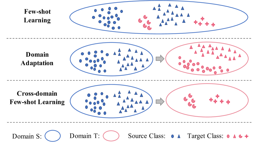
Figure 1. A comparison of few-shot learning, domain adaptation, and cross-domain few-shot learning is illustrated.

A comparison of FSL, domain adaption, and CD-FSL is shown in Figure 1. Essentially, CD-FSL is challenged in addressing the FSL and domain adaptation tasks, simultaneously. There is very little work proposed for CD-FSL. Recently, FWT (Tseng et al., 2020) proposes a feature-wise transformation layer to improve the generalization ability of the model. The hyper-parameters of the transformation layers are either manually tuned in a single-source setting or learned by constructing a pseudo-seen dataset and another pseudo-unseen dataset in a multiple-source setting. In this paper, we mainly focus on the single-source setting which is more practical in real-world applications. LRP-GNN (Sun et al., 2020) and SB-MTL (Cai et al., 2020) tackle this problem mainly by using the results of the explanation model and mapping the prediction scores onto a metric space, respectively. Another work (Phoo and Hariharan, 2020) supposes that a large number of unlabeled target examples are available. It is also a practical setting in some cases, particularly for analyzing medical images. But it may not be an easy task in many cases to collect so much unlabeled data such as fine-grained birds and plants.

Different from the previous works, this paper considers a more realistic scenario in CD-FSL. Particularly, in the CD-FSL task, the target classes always have a few labeled examples. We advocate utilizing these extremely few labeled target data (termed as the auxiliary dataset) to guide the meta-learning process. This has been proposed for two reasons. Firstly, without guidance from such target data, vanilla meta-learning algorithms may fail as both classes and domains are different between the source and the target datasets. Secondly, in practice, it may be much easier to label a few images than collect a large number of unlabeled images. Notably, all the images contained in the auxiliary dataset will not appear during the testing stage, thus we do not violate the basic CD-FSL setting.

Detailed pilot and feasibility studies are conducted under our new setting including 1) which training stage should the auxiliary data be used; 2) how the number of auxiliary data will affect the performance of our model. Our experimental results suggest the most appropriate training strategy under this setting and validate the soundness of our setting. A significant performance gain can be brought by introducing a small number of auxiliary target data.

Technically, we tackle this problem from two aspects. Firstly, a mixup module is re-proposed to make the best use of instances from the source and the newly introduced auxiliary datasets/domains. Mixing the images of two domains augments the auxiliary dataset to a large extent. Secondly, a disentangle module is proposed to decouple the image features into the disentangled domain-irrelevant and domain-specific features. The former ones are used to conduct the few-shot learning across the domains, while the latter ones contain significant inductive bias learned from the domains.

Formally, a novel network termed as meta-FDMixup (meta-learning based Feature-Distangled Mixup) is proposed in this paper. Specifically, for each training step, we first sample two episodes from the source and the auxiliary datasets, respectively. We then mix up the query images of the source episode with that of the auxiliary episode at a certain ratio. After that, our feature extractor and disentangle module learn to extract domain-irrelevant and domain-specific features for the source support set, the auxiliary support set, and the mixed query set, individually. Then, FSL classification tasks and domain classification tasks are performed. For FSL classification tasks, our FSL classifier is forced to classify the mixed query images into the class sets of the source support images and the auxiliary support images, given the domain-irrelevant features. For domain classification tasks, a domain classifier that aims at predicting the domain categories correctly only by domain-specific features is proposed. These two tasks are performed simultaneously.

Our contributions are summarized as follows. 1) For the first time, we advocate introducing extremely few labeled target data to guide the meta-learning process for the CD-FSL task. 2) Detailed pilot and feasibility studies are conducted for this new setting which reflect our intuitive understanding of CD-FSL, with the hope of igniting future research. 3) Technically, a novel meta-FDMixup network is proposed which utilizes the source and the newly introduced auxiliary data well by mixing the images and learns to disentangle the images features into the domain-irrelevant and the domain-specific ones, improving the model performance on both the source and the target domains. 4) The extensive experimental results validate the soundness of our new setting and the effectiveness of our proposed method.

2. Related Work

Few-shot Learning. Many efforts have been done to tackle the FSL problem. Existing few-shot learning methods mainly focus on model initialization (Finn et al., 2017; Rusu et al., 2018), metric-learning (Snell et al., 2017; Vinyals et al., 2016; Sung et al., 2018; Garcia and Bruna, 2017), and data augmentation (Chen et al., 2019a; Li et al., 2020b). More recent work includes cross-attention-based CAN (Hou et al., 2019), set-to-set function based FEAT (Ye et al., 2020), episodes relation based MELR (Fei et al., [n.d.]) and so on. One common point of the above methods is that they sample the source and the target images from the same dataset, intrinsically belonging to the same domain. Research (Chen et al., 2019b) points out that existing metric-learning based few-shot methods fail to generalize to the novel target classes when the source and the target data are sampled from different datasets. Thus, in this paper, we mainly stick to the metric-learning based methods and try to improve their performance under the cross-domain setting.

Domain Adaptation. Domain adaption aims at transferring knowledge from the source domain to the target domain which has the same class set while different data distribution from that of the source domain. Deep learning based methods can be roughly organized into three types: discrepancy based methods (Tzeng et al., 2014; Rozantsev et al., 2018; Kang et al., 2019), adversarial based methods (Tzeng et al., 2015; Ganin et al., 2016; Bousmalis et al., 2017), and reconstruction based methods (Bousmalis et al., 2016; Ghifary et al., 2016). Though our idea of extracting the domain-irrelevant features keeps the same with these domain adaptation methods, we are still different from them mainly in two aspects. Firstly, the class sets of the source and the target domains are the same in domain adaptation while disjoint in CD-FSL. Another point is that sufficient labeled or unlabeled target data can be used in the domain adaption task in general, while we have to classify the novel classes with few labeled data.

Cross-domain Few-shot Learning. Greatly promoted by the research (Chen et al., 2019b), the task of cross-domain few-shot learning is formally proposed in FWT (Tseng et al., 2020). Then, a new broader study together with a new benchmark is contributed by BSCD-FSL (Guo et al., 2020). Methods using only source data including FWT (Tseng et al., 2020), LRP-GNN (Sun et al., 2020) and SB-MTL (Cai et al., 2020). STARTUP (Phoo and Hariharan, 2020) relaxes the setting and assumes that the model has access to many unlabeled target data during training. Particularly, this paper resorts to a novel setting in that extremely few labeled target images are available. Comparing to the former strictly defined setting, a significant performance gain can be achieved with only a small number of labeled data. Comparing to the latter one, collecting extremely few labeled samples, e.g. 5 images per class, maybe easier and more practical than constructing a large amount of unlabeled data, especially in the case of fine-grained classes.

Data Augmentation. Recently, an advanced data augmentation termed as mixup (Zhang et al., 2017) is proposed to improve the robustness of the network. After that, several variants of mixup are proposed, including CutMix (Yun et al., 2019), Manifold Mixup (Verma et al., 2019), AugMix (Hendrycks et al., 2019), PuzzleMix (Kim et al., 2020) and so on. These mixup methods are designed for the classical classification task, which means that the mixed images come from the same class set and the model is trained with the standard cross-entropy loss. More related work to us is Xmixup (Li et al., 2020a) proposed for cross-domain transfer learning. Given a disjoint source and target dataset, XMixup assumes the source has more classes than the target. It first selects a unique source class for each target class, then applies mixup onto the one-to-one pairs. However, Xmixup still can not handle the few-shot learning problem.

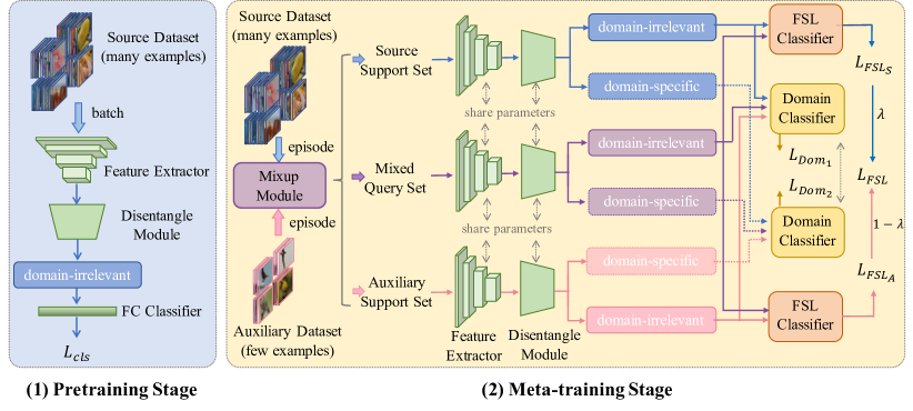
Figure 2. Overview of our framework. It mainly contains two stages. During the pretraining stage, we pretrain the feature extractor, the disentangle module, and the FC classifier with the supervised classification tasks. During the meta-training stage, we finetune the whole network with episode-based few-shot classification tasks in the meta-learning paradigm. To make use of the source and the newly introduced auxiliary datasets, a mixup module is re-proposed. Furthermore, to narrow the domain gap, we learn to disentangle the features by introducing a disentangle module and a domain classifier.

3. Method

3.1. Problem Formulation

Given the source dataset $D_{S}=\left\{\mathbf{I}_{j,}y_{j}\right\}_{j=1}^{n_{S}}$, of sufficient labeled images $y_{j}\in\mathcal{C}_{S}$, and a target data $D_{T}=\left\{\mathbf{I}_{j,}y_{j}\right\}_{j=1}^{n_{T}}$ with few labeled images, $y_{j}\in\mathcal{C}_{T}$. We have the disjointed source and target classes, i.e., $C_{S}\cap C_{T}=\emptyset$. Different from the standard few-shot learning where the $D_{S}$ and the $D_{T}$ are sampled from the same domain, the data distributions of the $D_{S}$ and the $D_{T}$ are different from each other in CD-FSL. The goal of our model is to learn the knowledge from the source dataset $D_{S}$ and transfer it to the target dataset $D_{T}$.

In the standard CD-FSL setting proposed by FWT (Tseng et al., 2020), the source dataset $D_{S}$ is further split into a source base $D_{S_{b}}$, a source eval $D_{S_{e}}$, and a source novel $D_{S_{n}}$. Similarly, the target dataset $D_{T}$ is split into a target base $D_{T_{b}}$, a target eval $D_{T_{e}}$, and a target novel $D_{T_{n}}$. The class sets of the base, the eval, and the novel datasets are disjointed from each other, again. During the experiments, the $D_{S_{b}}$, $D_{S_{e}}$, and $D_{T_{n}}$ serve as the training set, validation set, and testing set, respectively.

As for our new setting, we randomly sample $num_{target}$ labeled images per class from the target base dataset $D_{T_{b}}$. The selected target images together constitute our auxiliary dataset $D_{aux}$. Notably and most importantly, since the auxiliary dataset $D_{aux}$ comes from the target base dataset $D_{T_{b}}$ which is disjointed from the target testing set $C_{T_{n}}$, thus our setting does not violate the basic setting of CD-FSL.

N-way-K-shot Problem. To mimic the testing phase, meta-learning adopts an episode-based training mechanism. Each episode contains a support set $S=\left\{x_{i},y_{i}\right\}_{i=1}^{N\times K}$ and a query set $Q=\left\{x_{i},y_{i}\right\}_{i=1}^{N\times M}$. More specially, given a dataset, we first randomly sample $N$ classes, then for each selected class, K labeled images and another $M$ images are randomly sampled to constitute the support set and the query set, respectively. Our model learns to classify the labels of the query images according to the support set.

3.2. Meta-FDMixup Network

The illustration of our meta-FDMixup network is shown in Figure 2. Meta-FDMixup mainly consists of a feature extractor $f$, a disentangle module $h$, a FC classifier $g_{cls}$, a few-shot learning (FSL) classifier $g_{fsl}$, and a domain classifier $g_{dom}$. The according parameters are denoted as $\theta_{f}$, $\theta_{h}$, $\theta_{cls}$, $\theta_{fsl}$, and $\theta_{dom}$, respectively. The feature extractor $f$ extracts a 1-D feature representation $F$ for the input image. Principally, any image classification network can be introduced as the encoder. The disentangle module $h$ further decouples the extracted 1-D feature $F$ into a domain-irrelevant feature and a domain-specific feature. We use the $H1$ and $H2$ to denote the domain-irrelevant and the domain-specific features, respectively. The FC classifier $g_{cls}$ means a single fully connected layer that maps the extracted image representation to the scores on the source base classes $C_{S_{b}}$. The FSL classification $g_{fsl}$ takes a support set $S$ and a query set $Q$ as the input and is responsible for classifying the images in the query set according to the given support set. The domain classifier $g_{dom}$ learns to classify the input image into the source domain or the target domain. It works as the discriminator to supervise the learning process of the disentangle module.

A two-step training strategy is adopted to train the model. As for the pretraining stage, the batch data sampled from the source base dataset $D_{S_{b}}$ is fed into the feature extractor $f$ and the disentangle module $h$ successively. Then, the extracted domain-irrelevant feature $H1$ is fed into the FC classifier $g_{cls}$ to obtain its predictions on the source base classes $C_{S_{b}}$. The standard cross-entropy classification loss is used to train the network. During this process, the $\theta_{f}$, the $\theta_{h}$, and the $\theta_{cls}$ are optimized.

As for the meta-training stage, we train the whole network including the feature extractor $f$, the disentangle module $h$, the FSL classifier $g_{fsl}$, and the domain classifier $g_{dom}$ with the episode data under the meta-learning paradigm. For each training iteration, two episodes are randomly sampled from the source base dataset $D_{S_{b}}$ and the auxiliary dataset $D_{aux}$, respectively. In order to make the best use of the initial source data and the newly introduced auxiliary data, a simple yet effective mixup module is proposed which collaborates with the meta-learning mechanism. More specifically, given a source episode $E_{sou}$ and an auxiliary episode $E_{aux}$, we mix the images contained in the source query set $Q_{sou}$ with that in the auxiliary query set $Q_{aux}$ through linear combination at a ratio of $\lambda$.

(1) $$Q_{mix}=\lambda Q_{sou}+(1-\lambda)Q_{aux},$$

where the $Q_{mix}$ denotes the mixed query set, and the ratio $\lambda\sim Beta(\alpha,\alpha),\alpha\in(0,\infty)$ keeps the same as the mixup (Zhang et al., 2017).

Considering the FSL classification task requires a reliable support set, we keep the support sets of both the source episode and the auxiliary episode unchanged. The detailed illustration of our mixup module is shown in Figure 3. Formally, taking the source episode $E_{sou}$ and the auxiliary episode $E_{aux}$ as the input, our mixup module generates a source support set $S_{sou}$, an auxiliary support set $S_{aux}$, a mixed query set $Q_{mix}$, and the mixing ratio $\lambda$.

Figure 3. Illustration of our mixup module. We mix the query sets of the source and the auxiliary episodes at a ratio of $\lambda$ while keep the support sets of them unchanged.

After that, we feed the source support set $S_{sou}$, the auxiliary support set $S_{aux}$, and the mixed query set $Q_{mix}$ into the feature extractor $f$ and the disentangle module $h$ successively to obtain their domain-irrelevant features and domain-specific features. Take the mixed query set $Q_{mix}$ as an example, for each image contained, the feature extractor $f$ extracts a 1-D feature representation $F_{Q_{mix}}$. Then, the disentangle module further generates the domain-irrelevant feature $H1_{Q_{mix}}$ and the domain-specific feature $H2_{Q_{mix}}$ for the mixed query set $Q_{mix}$. In the same way, for the source and the auxiliary support sets, the domain-irrelevant features $H1_{S_{sou}}$, $H1_{S_{aux}}$ and the domain-specific features $H2_{S_{sou}}$, $H2_{S_{aux}}$ are generated.

The detailed illustration of the disentangled module $h$ is shown in Figure 4. It is mainly composed of a batch normalization layer, a relu activation layer, and several fully connected layers. More specifically, “FC1” is used to extract the general representation, while “FC21a” and “FC22a” are responsible for extracting the domain-irrelevant features – mean a and devia a. Correspondingly, the “FC21b” and “FC22b” are designed for extracting the domain-specific features. We highlight that our disentangle module is inspired but very different from VAE (Variation Auto-Encoder). Particularly, VAE only encodes one latent feature, while the key idea of our module lies in best learning to disentangle the domain-specific and domain-irrelevant features thus alleviating the domain shift problem in CD-FSL.

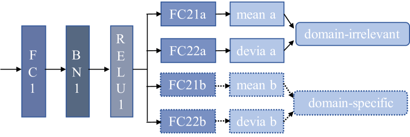
Figure 4. Architecture of our disentangle module.

In the end, a multi-task learning mechanism composed of FSL classification tasks and domain classification tasks is proposed to optimize our model. For FSL classification tasks, the domain-irrelevant features $H1_{S_{sou}}$, $H1_{S_{aux}}$, and $H1_{Q_{mix}}$ are used for classification. Recall that our query set is a mixture of the source query set and the auxiliary query set in the ratio $\lambda$, thus in our proposed meta-FDMixup method, the ratio $\lambda$ is considered as the confidence score of the mixed image belonging to its initial ground truth. More specifically, our FSL classifier is asked to classify the mixed query set into the class set of the source support set according to their features $H1_{Q_{mix}}$ and $H1_{S_{sou}}$ resulting in the FSL classification loss $\lambda L_{FSL_{S}}$. Similarly, the confidence score for classifying the mixed query set into the class set of auxiliary support set is $1-\lambda$, resulting in another FSL classification loss $(1-\lambda)L_{FSL_{A}}$. The $L_{FSL_{S}}$ and $L_{FSL_{A}}$ are generated by the FSL classifier. The FSL loss function is defined as follows,

(2) $$\mathcal{L}_{FSL}=\lambda\cdot\mathcal{L}_{FSL_{S}}+(1-\lambda)\mathcal{L}_{FSL_{A}}.$$

As for domain classification tasks, we hope the domain category can be easily identified given the domain-specific features $H2$ resulting in domain classification loss $L_{dom_{2}}$, while the domain-irrelevant features $H1$ are expected to confuse the domain classifier resulting in domain-classification loss $L_{dom_{1}}$. Our domain classifier contains a fully connected layer that maps the input feature into the scores on two domains.

Formally, let 1 and 0 denote the category of source and target, respectively. We define the ground truth for the domain-specific features $H2_{S_{sou}}$, $H2_{S_{aux}}$, $H2_{Q_{mix}}$ as $y2_{S_{sou}}\in\mathcal{R}^{NK}$, $y2_{S_{aux}}\in\mathcal{R}^{NK}$, $y2_{Q_{mix1}}\in\mathcal{R}^{NM}$, and $y2_{Q_{mix2}}\in\mathcal{R}^{NM}$, respectively. All the values in $y2_{S_{sou}}$ and $y2_{Q_{mix1}}$ are set as 1, all the values in $y2_{S_{aux}}$ and $y2_{Q_{mix2}}$ are set as 0.

(3) $$\mathcal{L}_{dom_{2}}=\frac{1}{3}\sum\left[\mathrm{CE}\left(g_{dom}(H2_{S_{sou}}),y2_{S_{sou}}\right)\right.$$

(4) $$+\,\mathrm{CE}\left(g_{dom}(H2_{S_{aux}}),y2_{S_{aux}}\right)$$

(5) $$+\,\lambda\cdot\mathrm{CE}\left(g_{dom}(H2_{Q_{mix}}),y2_{S_{mix1}}\right)$$

(6) $$+\left.(1-\lambda)\cdot\mathrm{CE}\left(g_{dom}(H2_{Q_{mix}}),y2_{S_{mix2}}\right)\right]$$

Similarly, we define the corresponding ground truth for the domain-irrelevant features $H1_{S_{sou}}$, $H1_{S_{aux}}$, $H1_{Q_{mix}}$ as $y1_{S_{sou}}\in\mathcal{R}^{NK\times 2}$, $y1_{S_{aux}}\in\mathcal{R}^{NK\times 2}$, $y1_{Q_{mix}}\in\mathcal{R}^{NM\times 2}$. All the lines in $y1_{S_{sou}}$, $y1_{S_{aux}}$, and $y1_{Q_{mix}}$ are set to $[0.5,0.5]$.

(7) $$\mathcal{L}_{dom_{1}}=\frac{1}{3}\sum\left[\mathrm{KL}\left(g_{dom}(H1_{S_{sou}}),y1_{S_{sou}}\right)\right.$$

(8) $$+\,\mathrm{KL}\left(g_{dom}(H1_{S_{aux}}),y1_{S_{aux}}\right)$$

(9) $$+\,\left.\mathrm{KL}\left(g_{dom}(H1_{Q_{mix}}),y1_{Q_{mix}}\right)\right]$$

The $CE()$ and the $KL()$ denotes the cross-entropy loss and the Kullback-Leibler divergence loss, respectively. These sub-tasks are performed in parallel in an end-to-end way. Our final loss function is defined as,

(10) $$\mathcal{L}=\mathcal{L}_{FSL}+\mathcal{L}_{dom_{2}}+\mathcal{L}_{dom_{1}}$$

5-way-5-shot	$D_{aux}$	stage	CUB	Cars	Places	Plantae
s-base	-	/	62.25 $\pm$ 0.65	44.28 $\pm$ 0.63	70.84 $\pm$ 0.65	52.53 $\pm$ 0.59
a-base	✓	P1+2	60.26 $\pm$ 0.71	40.43 $\pm$ 0.60	56.86 $\pm$ 0.67	53.88 $\pm$ 0.70
	✓	P2	64.98 $\pm$ 0.67	48.53 $\pm$ 0.64	67.96 $\pm$ 0.68	60.21 $\pm$ 0.69
m-base	✓	P1+2	77.07 $\pm$ 0.65	62.98 $\pm$ 0.69	76.08 $\pm$ 0.62	64.33 $\pm$ 0.69
	✓	P2	78.08 $\pm$ 0.60	63.27 $\pm$ 0.70	75.90 $\pm$ 0.67	66.69 $\pm$ 0.68

Table 1. Pilot study of different training strategies. The accuracy (%) is reported with GNN as the few-shot classifier. We compare our strategy (P2) with the two-step strategy (P1+2).

4. Experiments

Networks Components. To make a fair comparison with the FWT (Tseng et al., 2020), we follow the basic setup used in their work. For the feature encoder, Resnet-10 (He et al., 2016) is selected. For the FSL classifier, the GNN (Garcia and Bruna, 2017) is adopted. For the disentangle module, the input dim and the output dim of the FC1 are set as 512 and 256, respectively. All the FC21a, FC22a, FC21b, FC22b map the 256-D feature into a 64-D feature. The domain classifier further maps the 64-D feature into a 2-D vector.

Datasets. Mini-Imagenet (Ravi and Larochelle, 2017) serves as the source dataset $D_{S}$, and another four datasets including CUB (Wah et al., 2011), Cars (Krause et al., 2013), Places (Zhou et al., 2017), and Plantae (Van Horn et al., 2018) server as the target dataset $D_{T}$, respectively.

We follow the same base/eval/novel splits provided by FWT (Tseng et al., 2020). However, in our setting, a small part of the target base set $D_{T_{b}}$ is used at the training stage.

Implementation Details. The $num_{target}$ is set as 5 unless otherwise specified. The $\alpha$ is set as 1. Whether for which training stage, we train the network for 400 epochs. Notably, for miniImagenet, the model which performs best on the validation set $D_{S_{e}}$ is saved for testing; For all the target datasets, considering the domain gap, we uniformly use the last model for testing. The Adam with an initial learning rate of 0.001 is used as the optimizer. We conduct experiments on the 5-way-K-shot setting. The average accuracy of 1000 episodes is reported as the final result.

Baselines and Competitors. Several baselines and competitors are compared as follows. (1) To show the performance of the existing FSL methods on this CD-FSL setting, several flagship FSL methods including MatchingNet (Vinyals et al., 2016), RelationNet (Sung et al., 2018), and GNN (Garcia and Bruna, 2017) are introduced. For these methods, no auxiliary images are given. We unify the feature extractor as ResNet-10 for them following FWT (Tseng et al., 2020). (2) The GNN is adopted as the FSL classifier for all the other baselines and CD-FSL methods due to its good performance in the CD-FSL setting. Based on the ResNet-10 (feature extractor) and the GNN (FSL classifier), we build several baselines to show the effectiveness of the introduced auxiliary data. For “s-base”, we meta-train the network with the mini-Imagenet lonely. Thus, it equals the original GNN. Correspondingly, for “a-base”, the network is meta-trained with the auxiliary target data along. For our strong baseline “m-base”, the images of the mini-Imagenet and the auxiliary dataset are merged to train the model. (3) As for CD-FSL competitors, since the task is recently proposed, we only study FWT (Tseng et al., 2020). A novel feature-wise transformation layer is proposed in FWT which learns the scale and shift hyper-parameters of the batch normalization layer. In a single-source setting, the hyper-parameters are manually defined (FT) according to the empirical results. We use the hyper-parameters provided by FWT and integrate this method into our strong baseline “m-base” resulting in the competitor “m-base-FT”. Notably, only the mini-Imagenet is used during the first pretraining stage for all the methods, which will be explained in the following subsection.

4.1. Pilot & Feasibility Study

Considering there are two training stages, we first conduct a pilot study on which training stage should the auxiliary data be used. In addition, to validate the practicability of the proposed setting, we conduct a detailed feasibility study on how the number of auxiliary images affects the performance of the model.

In which training stage should the auxiliary images be used? As we stated in the sec 3, there are two training stages: 1) pretraining the feature encoder; 2) meta-training the whole model. We compare the two-stage strategy (denoted as “P1+2”) which uses the auxiliary images to train the model in both stages with “P2” which only uses the auxiliary data in the second meta-training stage. We conduct experiments on two different baselines, including “a-base” and “m-base”. The results of the “s-base” are taken as the baseline.

The results under the 5-way-5-shot setting are shown in Table 1. We notice that no matter which method is used, the “P2” strategy outperforms the “P1+2”. The only exception is marked in blue font in which “P1+2” shows a negligible advantage over “P2”. This phenomenon indicates that the feature extractor trained with the mini-Imagenet has a stronger ability to extract image representations. Using the auxiliary data in the pretraining stage may cause some noises thus damaging the performance of the whole model.

Is this setting feasible and how many examples should be provided? To answer this question, we set the $num_{target}$ as 5, 10, 15, and 20 to study how the performance will be affected as the number of labeled images increases. The results of our meta-FDMixup method are reported in Figure 5. Take CUB as an example, 17.21%, 24.42%, 26.50%, 27.04% performance gain is achieved with $num_{target}$ equals to 5, 10, 15 and 20, respectively. These results validate the feasibility and soundness of our new setting.

As for the most appropriate $num_{target}$, generally, the performance of the model is positively correlated with the number of labeled examples which keeps consistent with our common sense. However, we also observe that as the number of labeled examples increases, the performance improvement it brings slows down. This can be intuitively understood by the law of diminishing marginal utility. Take CUB as an example again, we denote 5 labeled images as a unit, the accuracy is improved by 17.21%, 7.21%, 2.08%, 0.54% by introducing the 1-st, 2-st, 3-st, and the 4-st unit, respectively. To trade off the performance and the labeling cost, we set $num_{target}$ as 5 in all of our experiments.

4.2. Main Results

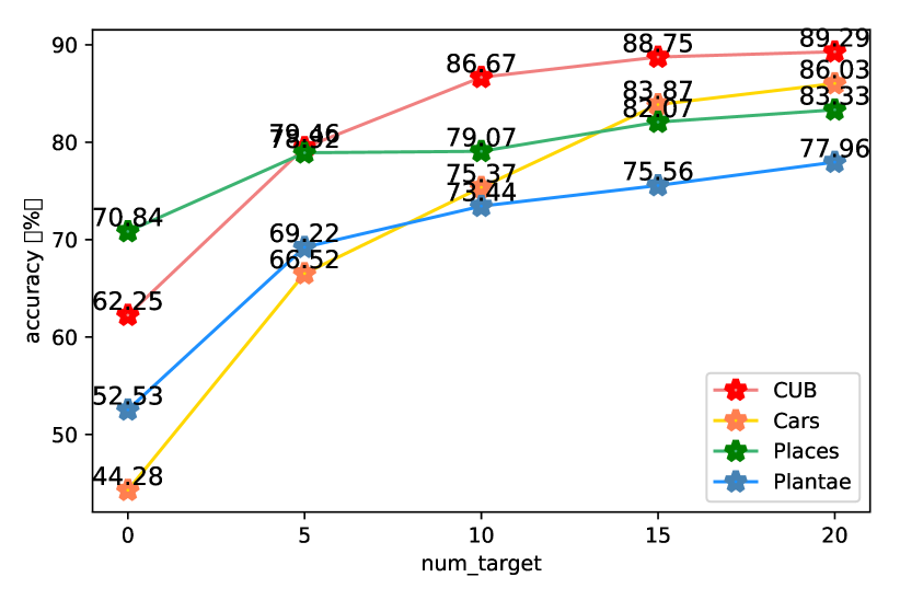
Figure 5. Feasibility study of our new setting. The accuracy (%) of our meta-FDMixup method under the 5-way-5-shot setting is reported. We set the $num_{target}$ as 5, 10, 15, and 20.

5-way	1-shot	$D_{aux}$	CUB	Cars	Places	Plantae
FSL	MatchingNet (Vinyals et al., 2016)	-	35.89 $\pm$ 0.51	30.77 $\pm$ 0.47	49.86 $\pm$ 0.79	32.70 $\pm$ 0.60
	RelationNet (Sung et al., 2018)	-	42.44 $\pm$ 0.77	29.11 $\pm$ 0.60	48.64 $\pm$ 0.85	33.17 $\pm$ 0.64
	GNN (Garcia and Bruna, 2017)	-	45.69 $\pm$ 0.68	31.79 $\pm$ 0.51	53.10 $\pm$ 0.80	35.60 $\pm$ 0.56
Baselines	s-base	-	45.69 $\pm$ 0.68	31.79 $\pm$ 0.51	53.10 $\pm$ 0.80	35.60 $\pm$ 0.56
	a-base	✓	50.28 $\pm$ 0.77	37.86 $\pm$ 0.63	51.09 $\pm$ 0.79	44.25 $\pm$ 0.74
	m-base	✓	57.65 $\pm$ 0.80	46.03 $\pm$ 0.72	55.70 $\pm$ 0.79	48.25 $\pm$ 0.74
CD-FSL	m-base-FT (Tseng et al., 2020)	✓	61.16 $\pm$ 0.81	49.01 $\pm$ 0.76	57.89 $\pm$ 0.82	50.49 $\pm$ 0.81
	meta-FDMixup (ours)	✓	63.24 $\pm$ 0.82	51.31 $\pm$ 0.83	58.22 $\pm$ 0.82	51.03 $\pm$ 0.81
5-way	5-shot	$D_{aux}$	CUB	Cars	Places	Plantae
FSL	MatchingNet (Vinyals et al., 2016)	-	51.37 $\pm$ 0.77	38.99 $\pm$ 0.64	63.16 $\pm$ 0.77	46.53 $\pm$ 0.68
	RelationNet (Sung et al., 2018)	-	57.77 $\pm$ 0.69	37.33 $\pm$ 0.68	63.32 $\pm$ 0.76	44.00 $\pm$ 0.60
	GNN (Garcia and Bruna, 2017)	-	62.25 $\pm$ 0.65	44.28 $\pm$ 0.63	70.84 $\pm$ 0.65	52.53 $\pm$ 0.59
Baselines	s-base	-	62.25 $\pm$ 0.65	44.28 $\pm$ 0.63	70.84 $\pm$ 0.65	52.53 $\pm$ 0.59
	a-base	✓	64.98 $\pm$ 0.67	48.53 $\pm$ 0.64	67.96 $\pm$ 0.68	60.21 $\pm$ 0.69
	m-base	✓	78.08 $\pm$ 0.60	63.27 $\pm$ 0.70	75.90 $\pm$ 0.67	66.69 $\pm$ 0.68
CD-FSL	m-base-FT (Tseng et al., 2020)	✓	79.14 $\pm$ 0.62	65.42 $\pm$ 0.70	78.59 $\pm$ 0.60	68.26 $\pm$ 0.68
	meta-FDMixup (ours)	✓	79.46 $\pm$ 0.63	66.52 $\pm$ 0.70	78.92 $\pm$ 0.63	69.22 $\pm$ 0.65

Table 2. The accuracy (%) under the 5-way-1shot and 5-way-5-shot settings are reported. For all the baselines and CD-FSL methods, GNN is adopted as the FSL classifier. Our meta-FDMixup method performs best.

target set	mini-Imagnet $|$ CUB	mini-Imagenet $|$ Cars	mini-Imagnet $|$ Places	mini-Imagnet $|$ Plantae
s-base	80.87 $\pm$ 0.56	80.87 $\pm$ 0.56	80.87 $\pm$ 0.56	80.87 $\pm$ 0.56
a-base	57.83 $\pm$ 0.63	50.04 $\pm$ 0.59	64.15 $\pm$ 0.69	53.20 $\pm$ 0.63
m-base	78.94 $\pm$ 0.58	80.75 $\pm$ 0.55	79.99 $\pm$ 0.58	80.51 $\pm$ 0.55
m-base-FT	81.88 $\pm$ 0.57	80.89 $\pm$ 0.58	81.32 $\pm$ 0.56	82.28 $\pm$ 0.55
ours	82.29 $\pm$ 0.57	81.00 $\pm$ 0.58	81.37 $\pm$ 0.56	79.64 $\pm$ 0.59

Table 3. Results (%) on the testing set of mini-ImagenetNet. The experiments are conducted under 5-way-5-shot setting taking GNN as the FSL classifier. Our method outperforms the baselines and competitors in most cases.

	single FSL classification task VS dual FSL classification tasks.
setting	$D_{aux}$	avg mini-ImageNet	CUB	Cars	Places	Plantae
$L_{FSL}=L_{FSL_{S}}$	✓	77.45 $\pm$ 0.63	46.08 $\pm$ 0.57	34.15 $\pm$ 0.53	65.41 $\pm$ 0.72	41.19 $\pm$ 0.60
$L_{FSL}=L_{FSL_{A}}$	✓	45.94 $\pm$ 0.58	74.18 $\pm$ 0.63	64.03 $\pm$ 0.71	67.51 $\pm$ 0.67	63.38 $\pm$ 0.69
meta-FDMixup	✓	81.08 $\pm$ 0.58	79.46 $\pm$ 0.63	66.52 $\pm$ 0.70	78.92 $\pm$ 0.63	69.22 $\pm$ 0.65
	different strategies for $\lambda$
setting	$D_{aux}$	avg mini-Imagenet	CUB	Cars	Places	Plantae
$\lambda$-v1	✓	78.02 $\pm$ 0.60	78.21 $\pm$ 0.63	63.85 $\pm$ 0.70	76.51 $\pm$ 0.65	67.87 $\pm$ 0.72
$\lambda$-v2	✓	80.78 $\pm$ 0.58	78.69 $\pm$ 0.63	60.65 $\pm$ 0.71	78.58 $\pm$ 0.63	66.91 $\pm$ 0.74
meta-FDMixup	✓	81.08 $\pm$ 0.58	79.46 $\pm$ 0.63	66.52 $\pm$ 0.70	78.92 $\pm$ 0.63	69.22 $\pm$ 0.65

Table 4. Ablation study on different FSL loss functions and different strategies for $\lambda$. The accuracy (%) with GNN as the classifier under the 5-way-5-shot setting is reported.

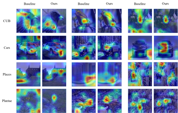
Figure 6. Grad-CAM visualization results of the “baseline” model and “ours” model. For each target dataset, three examples are demonstrated. Our model meta-finetuned with the help of the auxiliary data can focus on the key areas of the target images.

To show the effectiveness of our meta-FDMixup method, we compare it against all the baselines and competitors under the 5-way-1-shot and the 5-way-5-shot settings taking GNN as the FSL classifier. The results on the four target datasets are reported in Table 2.

Besides, we also report 5-way-5-shot classification results on the mini-Imagenet dataset in Table 3. Since our trained model is target set specific, our results are reported in the form of “mini-Imagenet $|$ target set”. “S-base” is the only exception, its results on the mini-Imagenet are not affected by the target set.

We highlight several points. 1) Comparing different FSL classifiers, the GNN performs best under this CD-FSL setting. It outperforms the Matching Net and the Relation Net by 10.88% and 4.48% on the CUB dataset under the 5-way-5-shot setting, respectively. Thus, we take the GNN as our FSL classifier. 2) The “s-base” baseline reaches a relatively good performance on the mini-Imagenet while fails to generalize to the target datasets with a sharp performance drop caused by the domain shift problem. 3) The “a-base” baseline performs better than “s-base” on the target datasets in most cases since it is meta-trained on the auxiliary dataset. However, its performance on the mini-Imagenet drops dramatically indicating that it suffers from the catastrophic forgetting problem. 4) Comparing with “s-base”, an obvious performance gain is brought by our strong baseline “m-base” on the target datasets. Take the GNN classifier under 5-way-5-shot as an example, we improve the accuracy by 15.83%, 18.99%, 5.06%, and 14.16% on CUB, Cars, Places, and Plantae datasets, respectively. We show that our setting brings very considerable benefits with only extremely few labeled data introduced. 5) Another observation worth mentioning about the “m-base” is that though it performs well on the target dataset, the ability to recognize the initial mini-Imagenet is damaged. That is because merging the relatively large-scale mini-Imagenet with the small-scale auxiliary dataset may cause the data imbalance problem. Not to mention, they belong to different domains. 6) For the competitor “m-base-FT”, we notice that it steadily improve the performance of the model on both the source and the target datasets which indicates its effectiveness. However, manually fine-tuning the hyper-parameters needs a lot of human labor, while our method is learned automatically. 7) Our method outperforms all the above methods on the source dataset and the different target datasets. Under the 5-way-5-shot setting, our meta-FDMixup achieves 79.46%, 66.52%, 78.92%, 69.22% on CUB, Cars, Places, and Plantae, respectively. Most importantly, the aforementioned problems encountered when using the small-regime auxiliary dataset are tackled by our meta-FDMixup.

Our mixup module enables us to mix the images from different domains resulting in massive and diverse mixed images. Our disentangle module learns to decouple the domain-irrelevant feature and the domain-specific feature, thus avoiding the influence of the domain shift. As a result, we not only achieve the best performance on the target datasets but also improve the accuracy on the mini-Imagenet dataset, which is actually out of our expectations.

4.3. Ablation Study

We first explore the effectiveness of our dual FSL classification task learning mechanism, then study the impact of $\lambda$ on our meta-FDMixup method. We conduct the experiments taking GNN as the classifier under the 5-way-5-shot learning setting. The results are demonstrated in Table 4. Notably, due to the limitation of the manuscript, the average accuracy on mini-ImageNet given different target datasets is reported.

Single FSL classification task VS dual FSL classification tasks. We compare our mechanism of dual few-shot classification tasks with that of single task. Specifically, to shown the performance of single FSL task, we define our FSL classification loss function as “$L_{FSL}=L_{FSL_{S}}$ ” and “$L_{FSL}=L_{FSL_{A}}$ ”, respectively. The results are shown in the first part of Table 4. An interesting phenomenon is that the single task mechanism is inferior to our multi-task mechanism even on its goal dataset. This observation in turn indicates that our multi-task mechanism makes the source and the target datasets promote each other mutually.

Different strategies for $\lambda$. In our meta-FDMixup, the $\lambda\sim Beta(\alpha,\alpha)$ treating the mini-Imagenet and the auxiliary data equally. We are wondering what would happen if we assign a higher ratio to one of these two datasets. In the end, two simple experiments are conducted. For “$\lambda$-v1”, if the value of $\lambda$ is higher than 0.5, we adjust it to 0.5, which means we want to ensure more than half of the auxiliary data will be maintained in the mixed data. Similarly, for “$\lambda$-v2”, we set the $\lambda$ to 0.5 if it is smaller than 0.5. The results are shown in the second part of Table 4. We notice that the accuracy of the target set decreases in both cases. For “$\lambda$-v2” it is easy to understand since it tends to protect the mini-Imagenet data. One reason that causes the performance drop for the “$\lambda$-v1” may be that the diversity of the mixed data is also reduced with a smaller ratio of mini-Imagenet.

4.4. Visualization Results

To provide a more intuitive understanding of our new setting – introducing some auxiliary target images to the training stage, we visualize the class-activation map of “baseline” and “ours” using the grad-CAM (Selvaraju et al., 2017). “Baseline” refers to the model pretrained on the mini-ImageNet dataset. It is composed of the feature encoder, the disentangle module, and the FC classifier. “Ours” denotes our meta-FDMixup model further meta-finetuned on the source dataset and the auxiliary dataset. For each target dataset, three examples are sampled from the testing set to give a comparison between the “baseline” and the “ours”. The results are shown in Figure 6.

Several phenomenons can be observed. 1) Generally, the “baseline” model pays more attention to the things which are more common in the mini-Imagenet, such as the branches in the CUB dataset, the mountains in the Cars dataset, and some backgrounds in the Places and the Plantae datasets. This will damage the model performance in the target datasets. However, without any target dataset, it is difficult to generalize to the target datasets well. 2) “Ours” model alleviates this problem to some extent. We successfully move the model’s attention to those areas that are critical for identifying the target classes. Take the CUB dataset as an example, our model focuses on the key parts of the birds, such as the feathers and the tails.

5. Conclusion

In this paper, to tackle the domain shift problem in CD-FSL, we advocate utilizing extremely few labeled target data for cross-domain few-shot learning. The detailed pilot and feasibility and studies explore the most suitable training strategy and validate the soundness of our new setting. Technically, a novel meta-FDMixup network that collaborates with meta-learning is proposed by us. By mixing the images of the source and the target datasets and learning to disentangle the domain-irrelevant and domain-specific features, our meta-FDMixup model can be well generalized to the target datasets. Extensive experiments show the effectiveness of our method.

6. Acknowledgement

This work was supported by National Natural Science Foundation of China Project (62072116) and Science and Technology Commission of Shanghai Municipality Projects (19511120700, 19ZR1471800).

References

- (1)
- Bousmalis et al. (2017) Konstantinos Bousmalis, Nathan Silberman, David Dohan, Dumitru Erhan, and Dilip Krishnan. 2017. Unsupervised pixel-level domain adaptation with generative adversarial networks. In CVPR.
- Bousmalis et al. (2016) Konstantinos Bousmalis, George Trigeorgis, Nathan Silberman, Dilip Krishnan, and Dumitru Erhan. 2016. Domain separation networks. arXiv preprint (2016).
- Cai et al. (2020) John Cai, Bill Cai, and Sheng Mei Shen. 2020. SB-MTL: Score-based Meta Transfer-Learning for Cross-Domain Few-Shot Learning. arXiv preprint arXiv:2012.01784 (2020).
- Chen et al. (2019b) Wei-Yu Chen, Yen-Cheng Liu, Zsolt Kira, Yu-Chiang Frank Wang, and Jia-Bin Huang. 2019b. A closer look at few-shot classification. arXiv preprint (2019).
- Chen et al. (2019a) Zitian Chen, Yanwei Fu, Kaiyu Chen, and Yu-Gang Jiang. 2019a. Image block augmentation for one-shot learning. In AAAI.
- Fei et al. ([n.d.]) Nanyi Fei, Zhiwu Lu, Tao Xiang, and Songfang Huang. [n.d.]. MELR: Meta-Learning via Modeling Episode-level Relationships for Few-shot Learning. ([n. d.]).
- Finn et al. (2017) Chelsea Finn, Pieter Abbeel, and Sergey Levine. 2017. Model-agnostic meta-learning for fast adaptation of deep networks. arXiv preprint (2017).
- Ganin et al. (2016) Yaroslav Ganin, Evgeniya Ustinova, Hana Ajakan, Pascal Germain, Hugo Larochelle, François Laviolette, Mario Marchand, and Victor Lempitsky. 2016. Domain-adversarial training of neural networks. JMLR (2016).
- Garcia and Bruna (2017) Victor Garcia and Joan Bruna. 2017. Few-shot learning with graph neural networks. arXiv preprint (2017).
- Ghifary et al. (2016) Muhammad Ghifary, W Bastiaan Kleijn, Mengjie Zhang, David Balduzzi, and Wen Li. 2016. Deep reconstruction-classification networks for unsupervised domain adaptation. In ECCV.
- Guo et al. (2020) Yunhui Guo, Noel C Codella, Leonid Karlinsky, James V Codella, John R Smith, Kate Saenko, Tajana Rosing, and Rogerio Feris. 2020. A broader study of cross-domain few-shot learning. In ECCV.
- He et al. (2016) Kaiming He, Xiangyu Zhang, Shaoqing Ren, and Jian Sun. 2016. Deep residual learning for image recognition. In CVPR.
- Hendrycks et al. (2019) Dan Hendrycks, Norman Mu, Ekin D Cubuk, Barret Zoph, Justin Gilmer, and Balaji Lakshminarayanan. 2019. Augmix: A simple data processing method to improve robustness and uncertainty. arXiv preprint arXiv:1912.02781 (2019).
- Hou et al. (2019) Ruibing Hou, Hong Chang, Bingpeng Ma, Shiguang Shan, and Xilin Chen. 2019. Cross attention network for few-shot classification. arXiv preprint arXiv:1910.07677 (2019).
- Kang et al. (2019) Guoliang Kang, Lu Jiang, Yi Yang, and Alexander G Hauptmann. 2019. Contrastive adaptation network for unsupervised domain adaptation. In CVPR.
- Kim et al. (2020) Jang-Hyun Kim, Wonho Choo, and Hyun Oh Song. 2020. Puzzle mix: Exploiting saliency and local statistics for optimal mixup. In International Conference on Machine Learning. PMLR, 5275–5285.
- Krause et al. (2013) Jonathan Krause, Michael Stark, Jia Deng, and Li Fei-Fei. 2013. 3d object representations for fine-grained categorization. In ICCVW.
- Li et al. (2020b) Kai Li, Yulun Zhang, Kunpeng Li, and Yun Fu. 2020b. Adversarial Feature Hallucination Networks for Few-Shot Learning. In CVPR.
- Li et al. (2020a) Xingjian Li, Haoyi Xiong, Haozhe An, Chengzhong Xu, and Dejing Dou. 2020a. XMixup: Efficient Transfer Learning with Auxiliary Samples by Cross-domain Mixup. arXiv preprint (2020).
- Phoo and Hariharan (2020) Cheng Perng Phoo and Bharath Hariharan. 2020. Self-training for Few-shot Transfer Across Extreme Task Differences. arXiv preprint (2020).
- Ravi and Larochelle (2017) Sachin Ravi and Hugo Larochelle. 2017. Optimization as a model for few-shot learning. In ICLR.
- Rozantsev et al. (2018) Artem Rozantsev, Mathieu Salzmann, and Pascal Fua. 2018. Beyond sharing weights for deep domain adaptation. TPAMI (2018).
- Rusu et al. (2018) Andrei A Rusu, Dushyant Rao, Jakub Sygnowski, Oriol Vinyals, Razvan Pascanu, Simon Osindero, and Raia Hadsell. 2018. Meta-learning with latent embedding optimization. arXiv preprint (2018).
- Selvaraju et al. (2017) Ramprasaath R Selvaraju, Michael Cogswell, Abhishek Das, Ramakrishna Vedantam, Devi Parikh, and Dhruv Batra. 2017. Grad-cam: Visual explanations from deep networks via gradient-based localization. In Proceedings of the IEEE international conference on computer vision. 618–626.
- Snell et al. (2017) Jake Snell, Kevin Swersky, and Richard Zemel. 2017. Prototypical networks for few-shot learning. In NeurIPS.
- Sun et al. (2020) Jiamei Sun, Sebastian Lapuschkin, Wojciech Samek, Yunqing Zhao, Ngai-Man Cheung, and Alexander Binder. 2020. Explanation-guided training for cross-domain few-shot classification. arXiv preprint (2020).
- Sung et al. (2018) Flood Sung, Yongxin Yang, Li Zhang, Tao Xiang, Philip HS Torr, and Timothy M Hospedales. 2018. Learning to compare: Relation network for few-shot learning. In CVPR.
- Tseng et al. (2020) Hung-Yu Tseng, Hsin-Ying Lee, Jia-Bin Huang, and Ming-Hsuan Yang. 2020. Cross-domain few-shot classification via learned feature-wise transformation. In ICLR.
- Tzeng et al. (2015) Eric Tzeng, Judy Hoffman, Trevor Darrell, and Kate Saenko. 2015. Simultaneous deep transfer across domains and tasks. In ICCV.
- Tzeng et al. (2014) Eric Tzeng, Judy Hoffman, Ning Zhang, Kate Saenko, and Trevor Darrell. 2014. Deep domain confusion: Maximizing for domain invariance. arXiv preprint (2014).
- Van Horn et al. (2018) Grant Van Horn, Oisin Mac Aodha, Yang Song, Yin Cui, Chen Sun, Alex Shepard, Hartwig Adam, Pietro Perona, and Serge Belongie. 2018. The inaturalist species classification and detection dataset. In CVPR.
- Verma et al. (2019) Vikas Verma, Alex Lamb, Christopher Beckham, Amir Najafi, Ioannis Mitliagkas, David Lopez-Paz, and Yoshua Bengio. 2019. Manifold mixup: Better representations by interpolating hidden states. In ICML.
- Vinyals et al. (2016) Oriol Vinyals, Charles Blundell, Timothy Lillicrap, Daan Wierstra, et al. 2016. Matching networks for one shot learning. In NeurIPS.
- Wah et al. (2011) Catherine Wah, Steve Branson, Peter Welinder, Pietro Perona, and Serge Belongie. 2011. The caltech-ucsd birds-200-2011 dataset. (2011).
- Ye et al. (2020) Han-Jia Ye, Hexiang Hu, De-Chuan Zhan, and Fei Sha. 2020. Few-shot learning via embedding adaptation with set-to-set functions. In Proceedings of the IEEE/CVF Conference on Computer Vision and Pattern Recognition. 8808–8817.
- Yun et al. (2019) Sangdoo Yun, Dongyoon Han, Seong Joon Oh, Sanghyuk Chun, Junsuk Choe, and Youngjoon Yoo. 2019. Cutmix: Regularization strategy to train strong classifiers with localizable features. In ICCV.
- Zhang et al. (2017) Hongyi Zhang, Moustapha Cisse, Yann N Dauphin, and David Lopez-Paz. 2017. mixup: Beyond empirical risk minimization. arXiv preprint (2017).
- Zhou et al. (2017) Bolei Zhou, Agata Lapedriza, Aditya Khosla, Aude Oliva, and Antonio Torralba. 2017. Places: A 10 million image database for scene recognition. TPAMI (2017).