A Transductive Maximum Margin Classifier for Few-Shot Learning

Abstract

Few-shot learning aims to train a classifier that can generalize well when just a small number of labeled examples per class are given. We introduce a transductive maximum margin classifier for few-shot learning (FS-TMMC). The basic idea of the classical maximum margin classifier is to solve an optimal prediction function so that the training data can be correctly classified by the resulting classifer with the largest geometric margin. In few-shot learning, it is challenging to find such classifiers with good generalization ability due to the insufficiency of training data in the support set. FS-TMMC leverages the unlabeled query examples to adjust the separating hyperplane of the maximum margin classifier such that the prediction function is optimal on both the support and query sets. Furthermore, we use an efficient and effective quasi-Newton algorithm, the L-BFGS method for optimization. Experimental results on three standard few-shot learning benchmarks including miniImagenet, tieredImagenet and CUB show that our method achieves state-of-the-art performance.

Keywords transductive, few-shot learning, maximum margin classifier, separating hyperplane, L-BFGS

1 Introduction

In recent years, deep learning models have made remarkable progress in various vision and language tasks [1, 2, 3]. However, they have a common limitation, that training effective deep neural networks requires a great number of labeled examples. Besides, it is costly to collect and label the large amount of training data. In some situations, it is extremely difficult to obtain enough training data, such as medical image processing, scarce objects identification. When the training data is insufficient, the trained model is prone to overfitting. Notably, humans are capable of learning from a small number of examples by leveraging past experiences. Inspired by this, few-shot learning, which is designed to learn a new visual concept through a few training examples, is attracting more and more research attentions.

In order to alleviate the overfitting problem caused by the inadequate labeled data in few-shot learning, Vinyals et al. [4] propose an episodic training strategy to learn from diverse tasks over vast episodes. In each episode, the algorithm learns from a few labeled examples in the support set, which will be used to make predictions in the unlabeled query examples. This learning strategy simulates the evaluation phase where there are insufficient labeled examples as well as some unlabeled data. The consistency between the training and evaluation phases reduces generalization errors by alleviating the distribution gap [5]. It has been adopted by many approaches in few-shot learning [6, 7, 8, 9, 10]. However, this strategy cannot resolve the problem of learning from inadquate training data.

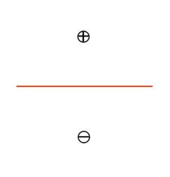
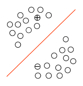
Figure 1: An example of the 2-way 1-shot problem where there are totally two categories and each category contains one example in the support set. The symbols +⃝, -⃝, ⃝ in the figure denote the labeled positive example, the labeled negative example and the unlabeled example, respectively. (a) The maximum margin classifier is solved with the support examples. (b) The query examples are also involved in solving the maximum margin classifier.

In this paper, we propose a transductive maximum margin classifier for few-shot learning (FS-TMMC). The classical maximum margin classifier aims to search for a predicton function so that the corresponding separating hyperplane correctly divides the training data and the resulting classifier has the largest geometric margin. In few-shot learning scenarios, the training examples are scarce, not enough to find a separating hyperplane that generalizes well on unseen data. FS-TMMC is constructed using a mixture of the labeled support examples and the unlabeled query examples in a given task. Different from the maximum margin classifier, the objective of FS-TMMC also involves assigning category labels to the query examples when constructing the maximum margin classifier. In order to obtain the labels of the query examples, we calculate the prediction function on the query set by taking advantage of both the support and query examples.

The involvement of the query examples in finding the optimal prediction function brings improvement to the maximum margin classifier because of the insufficiency of the training data in the support set. The unlabeled examples in the query set would adjust the separating hyperplane such that the prediction function is optimal on both the support and query examples. Please refer to Figure 1 for an example that illustrates the research motivation of FS-TMMC. Given the support examples only, the maximum margin classifier would produce an optimal separating hyperplane as illustrated by the solid red line in Figure 1(a). As shown in Figure 1(b), the unlabeled examples in the query set are also involved in solving the optimal prediction function of the maximum margin classifier. We observe that the normal vector of the resulting separating hyperplane in Figure 1(b) is distinct from that in Figure 1(a). Besides, the solved optimal prediction function in Figure 1(a) would produce a few misclassifications in the query set.

Our paper makes three main contributions. First, we propose a transductive maximum margin classifier for few-shot learning (FS-TMMC) which adjusts the separating hyperplane of the maximum margin classifier by taking account of information from the query examples. Second, we leverage the one-vs-rest strategy to make our problem compatible with the binary classification model and use Platt scaling to transform the output of the corresponding prediction function into a probability distribution over categories. Third, we evaluate our method on three benchmark datasets for few-shot learning, namely miniImageNet, tieredImageNet and CUB. The experimental results show that FS-TMMC achieves state-of-the-art results.

2 Related work

There are a variety of works on Few-Shot Learning which can be broadly categorized into five categories by prior knowledge representations.

Metric-based methods. Koch et al. [11] propose the Siamese Network to measure the similarity between the query and the support examples. Snell et al. [12] propose to use the class prototypes which are calculated by averaging the embeddings of the support examples from each category and make predictions based on the distances of the query example with respect to all prototypes. Triantafillou et al. [13] leverage the unlabeled examples when producing prototypes.

Memory-based methods. Santoro et al. [14] introduce MANN which originally uses memory networks to store feature and label pairs, and update elements with the least recently used strategy. MetaNet [15] stores model parameters in memory which are the fast weights for the support examples to help query examples get relevant information, and updates the parameters across tasks.

Optimization-based methods. MAML [6] learns good initialization of the parameters in the model. The model with the learned parameters may not perform well on the other tasks, but using these parameters as a starting point, it would learn from new tasks fast. Instead of adapting the high-dimensional model parameters through back propagation as in MAML [6], LEO [8] learns the parameters of an encoder and an decoder, and makes adaptations in the low-dimensional latent space.

Generation-based methods. RTA [16] produces parameters of neural networks based on the support examples in a task. But it only produces a part of the model parameters to adjust the network for the given task. LGM-Net [9] directly generates the parameters of the matching networks based on the latent representations of the examples in the support set.

Transductive methods. These methods construct the models using both the labeled and unlabeled examples, making full use of task information. TPN [5] learns to propagate labels by label propagation, and the weight matrix is obtained from learning. CAN-T [17] utilizes attention mechanisms to calculate the cross attention maps between the support and the query examples, making the extracted features more discriminant.

Similar to our method, several recent approaches deal with the problem of few-shot learning without episodic training. They train general classification networks on the base dataset, which will be used as feature extractors in the evaluation stage. SimpleShot [18] shows that a simple nearest-neighbor classifier with feature transformations and L2-normalization leads to competitive few-shot learning results. LaplacianShot [19] introduces a transductive inference algorithm that minimizes a Laplacian-regularized binary-assignment function to encourage similar examples to be assigned with the same labels. In contrast to the two approaches, our method leverages the examples in the query set to adjust the separating hyperplane of the maximum margin classifier.

3 Main Approach

3.1 Problem Setting

In few-shot image classification, there are three datasets with non-overlapping categories: the base set $\mathcal{D}_{base}$, the validation set $\mathcal{D}_{validation}$ and the test set $\mathcal{D}_{test}$. We train a general image classification model using the base set $\mathcal{D}_{base}$, which extracts the feature representations of the examples in the test set $\mathcal{D}_{test}$. The validation set $\mathcal{D}_{validation}$ is used to tune the hyper-parameters. In the evaluation stage of $N$-way $K$-shot tasks, we randomly sample $N$ categories from the test set $\mathcal{D}_{test}$ and $K$ examples from each category to construct the support set. Our approach is evaluated in the query set where $Q$ examples are provided for each category.

3.2 FS-TMMC

We begin by introducing the hinge loss function: $l(u)=\max(0,1-u)$. Support Vector Machines is the corresponding maximum margin classifier, which solves:

$$\mathop{{\rm minimize}}_{f\in\mathcal{H}}\ \frac{\lambda}{2}\|f\|_{\mathcal{H}}^{2}+\frac{1}{n}\sum_{i=1}^{n}l(y_{i}f(\bm{x}_{i})),$$ (1)

where $f$ lies in a Reproducing Kernel Hilbert Space $\mathcal{H}$, $y_{i}$ belongs to $\{-1,+1\}$, and $\lambda\ (\lambda>0)$ is a hyper-parameter.

We first train a base classification model with deep neural networks $g_{\bm{\theta}}$ parameterized by $\bm{\theta}$ using the base set $\mathcal{D}_{base}$. The output dimension of $g_{\bm{\theta}}$ is set to $D$. Then we sample $N$-way $K$-shot tasks from the test set $\mathcal{D}_{test}$. Each task contains a support set $\mathcal{S}=\{(Z_{i},y_{i})\}_{i=1}^{NK}$ and a query set $\mathcal{Q}=\{(Z_{i},y_{i})\}_{i=1}^{NQ}$. We leverage $g_{\bm{\theta}}$ to extract the compact feature representations of $\mathcal{S}$ and $\mathcal{Q}$ to obtain the pre-processed support set $\mathcal{S}^{\prime}=\{(\bm{z}_{i},y_{i})|\bm{z}_{i}=g_{\bm{\theta}}(Z_{i})$, $(Z_{i},y_{i})\in\mathcal{S},i=1,\cdots,NK\}$ and the pre-processed query set $\mathcal{Q}^{\prime}=\{(\bm{z}_{i},y_{i})|\bm{z}_{i}=g_{\bm{\theta}}(Z_{i})$, $(Z_{i},y_{i})\in\mathcal{Q},i=1,\cdots,NQ\}$. Besides, we define the following matrices:

$$\bm{X}_{\mathcal{S}^{\prime}} =[\bm{x}_{1},\cdots,\bm{x}_{NK}],$$ (2)

$$\bm{x}_{i} =\bm{z}_{i},\ (\bm{z}_{i},y_{i})\in\mathcal{S}^{\prime},\ i\in\{1,\cdots,NK\};$$

$$\bm{X}_{\mathcal{Q}^{\prime}} =[\bm{x}_{NK+1},\cdots,\bm{x}_{NK+NQ}],$$ (3)

$$\bm{x}_{NK+i} =\bm{z}_{i},\ (\bm{z}_{i},y_{i})\in\mathcal{Q}^{\prime},\ i\in\{1,\cdots,NQ\}.$$

We use the one-vs-rest strategy to make our problem compatible with the binary classification model. For each category $c\in\{1,\cdots,N\}$, we introduce a label vector of the support set $\bm{y}^{c}=[y_{1}^{c},\cdots,y_{NK}^{c}]^{T}\in R^{NK}$, where the value of $y_{i}^{c}$ is set to $+1$ if $y_{i}$ equals $c$ and $-1$ otherwise, $(\bm{z}_{i},y_{i})\in\mathcal{S}^{\prime},i\in\{1,\cdots,NK\}$.

Due to the introduction of the one-vs-rest strategy, the training examples of each category become unbalanced. So we assign category weights to all examples in the support set which are inversely proportional to category frequencies. The weight vector is $\bm{w}^{c}=[w_{1}^{c},w_{2}^{c},\cdots,w_{NK}^{c}]^{T}\in R^{NK}$.

In addition to the labeled data $\bm{X}_{\mathcal{S}^{\prime}}$, we also take advantage of the unlabeled examples $\bm{X}_{\mathcal{Q}^{\prime}}$ to get more accurate prediction functions [20, 21]. Specifically, we are intended to find the prediction function $f^{c}\in\mathcal{H}$ as well as the label assignments for the query examples $\bm{y}^{c\prime}=[y^{c\prime}_{1},\cdots,y^{c\prime}_{NQ}]^{T}$ by the following optimization problem:

$$\mathop{{\rm minimize}}_{f^{c}\in\mathcal{H},\bm{y}^{c\prime}}\ \frac{\lambda_{1}}{2}\|f^{c}\|_{\mathcal{H}}^{2}+\frac{1}{NK}\sum_{i=1}^{NK}w_{i}^{c}l(y_{i}^{c}f^{c}(\bm{x}_{i}))$$

$$+\lambda_{2}\frac{1}{NQ}\sum_{i=1}^{NQ}l(y^{c\prime}_{i}f^{c}(\bm{x}_{NK+i})),$$ (4)

where $\lambda_{1},\lambda_{2}\ (\lambda_{1},\lambda_{2}>0)$ are hyper-parameters.

The optimal value of $y^{c\prime}_{i}$ equals $1$ if $f^{c}(\bm{x}_{NK+i})\geq 0$ and $-1$ otherwise [22]. Thus we get the following optimization problem:

$$\mathop{{\rm minimize}}_{f^{c}\in\mathcal{H}}\ \frac{\lambda_{1}}{2}\|f^{c}\|_{\mathcal{H}}^{2}+\frac{1}{NK}\sum_{i=1}^{NK}w_{i}^{c}\max(0,1-y_{i}^{c}f^{c}(\bm{x}_{i}))$$

$$+\lambda_{2}\frac{1}{NQ}\sum_{i=1}^{NQ}\max(0,1-|f^{c}(\bm{x}_{NK+i})|).$$ (5)

Obviously, Eq. (3.2) contains the maximum and absolute value operations which are not differentiable. In order to optimize it efficiently, we replace the non-differentiable parts in Eq. (3.2) with their differentiable surrogates. Specifically, we use the LogSumExp function to approximate the maximum operator in the term $\max(0,1-y_{i}^{c}f(\bm{x}_{i}))$: $\max(a_{1},\cdots,a_{n})\approx\frac{1}{\gamma_{1}}\log\sum_{i=1}^{n}\exp{(\gamma_{1}a_{n})}$ [23]. Following Chapelle et al. [22], we replace the term $\max(0,1-|f^{c}(\bm{x}_{NK+i})|)$ by the term ${\rm exp}(-\gamma_{2}f^{c}(\bm{x}_{NK+i})^{2})$. $\gamma_{1},\gamma_{2}$ are used as hyperparameters.

According to the representer theorem [24], the solution of Eq. (3.2) satisfies

$$f^{c*}(\bm{x})=\sum_{i=1}^{M}\alpha^{c*}_{i}k(\bm{x}_{i},\bm{x}),$$ (6)

where the function $k$ is the reproducing kernel of $\mathcal{H}$ and $M$ equals $NK\!+\!NQ$. By introducing the vector $\bm{\alpha}^{c}=[\alpha_{1}^{c},\cdots,\alpha_{M}^{c}]^{T}$, $\bm{\alpha}^{c*}$ solves

$$\arg\min_{\bm{\alpha}^{c}}F(\bm{\alpha}^{c})=\frac{\lambda_{1}}{2}(\bm{\alpha}^{c})^{T}\bm{K}\bm{\alpha}^{c}$$

$$+\frac{1}{NK}\sum_{i=1}^{NK}\frac{w_{i}^{c}}{\gamma_{1}}\log(1+{\rm exp}(\gamma_{1}(1-y_{i}^{c}\sum_{j=1}^{M}\alpha^{c}_{j}k(\bm{x}_{j},\bm{x}_{i}))))$$

$$+\lambda_{2}\frac{1}{NQ}\sum_{i=1}^{NQ}{\rm exp}(-\gamma_{2}(\sum_{j=1}^{M}\alpha^{c}_{j}k(\bm{x}_{j},\bm{x}_{NK+i}))^{2}),$$ (7)

where $\bm{K}$ is a matrix with elements $K_{ij}=k(\bm{x}_{i},\bm{x}_{j})$, $i,j\in\{1,2,\cdots,M\}$.

The gradient of $F(\bm{\alpha}^{c})$ w.r.t. $\bm{\alpha}^{c}$ is

$$\nabla_{\bm{\alpha}^{c}}F(\bm{\alpha}^{c})=\bm{K}(\lambda_{1}\bm{\alpha}^{c}+\bm{t}),$$ (8)

where $\bm{t}\in{R}^{M}$ is a vector with elements

$$t_{i}=\left\{\begin{aligned} &-\frac{o_{i}}{p_{i}}&i\leq NK,\\ &-\frac{q_{i}}{NQ}&otherwise,\end{aligned}\right.$$ (9)

and

$$o_{i} =w_{i}^{c}y_{i}^{c}{\rm exp}(\gamma_{1}(1-y_{i}^{c}\sum_{j=1}^{M}\alpha^{c}_{j}k(\bm{x}_{j},\bm{x}_{i}))),$$

$$p_{i} =NK(1+{\rm exp}(\gamma_{1}(1-y_{i}^{c}\sum_{j=1}^{M}\alpha^{c}_{j}k(\bm{x}_{j},\bm{x}_{i})))),$$

$$q_{i} =2\gamma_{2}\lambda_{2}\sum_{j=1}^{M}\alpha^{c}_{j}k(\bm{x}_{j},\bm{x}_{i}){\rm exp}(-\gamma_{2}(\sum_{j=1}^{M}\alpha^{c}_{j}k(\bm{x}_{j},\bm{x}_{i}))^{2}).$$

3.3 Optimization

In order to optimize the proposed model efficiently, we use the BFGS algorithm which generates an approximate Hessian matrix at each step with a small computational cost. The iterative sequence generated by the approximate matrix rather than the Hessian matrix still has the property of superlinear convergence.

Given an initial $\bm{\alpha}_{0}^{c}\in{R}^{M}$, the BFGS algorithm calculates the sequence $\bm{\alpha}_{1}^{c},\cdots,\bm{\alpha}_{k}^{c},\bm{\alpha}_{k+1}^{c}$ iteratively until convergence via

$$\bm{\alpha}_{k+1}^{c}=\bm{\alpha}_{k}^{c}+t_{k}\bm{d}_{k}$$ (10)

where $t_{k}$ is the stepsize and the direciton $\bm{d}_{k}=-\bm{H}^{k}\nabla_{\bm{\alpha}^{c}}F(\bm{\alpha}_{k}^{c})$.

The update of the inverse Hessian approximation is given by [25]:

$$\bm{H}^{k+1}=(I-\rho_{k}\bm{s}_{k}\bm{w}_{k}^{T})\bm{H}^{k}(I-\rho_{k}\bm{w}_{k}\bm{s}_{k}^{T})+\rho_{k}\bm{s}_{k}\bm{s}_{k}^{T}$$ (11)

where $\rho_{k}=(\bm{w}_{k}^{T}\bm{s}_{k})^{-1}$, $\bm{w}_{k}=\nabla_{\bm{\alpha}^{c}}F(\bm{\alpha}_{k+1}^{c})-\nabla_{\bm{\alpha}^{c}}F(\bm{\alpha}_{k}^{c})$ and $\bm{s}_{k}=\bm{\alpha}_{k+1}^{c}-\bm{\alpha}_{k}^{c}$.

Although the BFGS method overcomes the difficulty of calculating the Hessian matrix, it still cannot be applied to large-scale optimization problems. Generally speaking, the inverse Hessian approximation $\bm{H}^{k}$ is a dense matrix, and storing the dense matrix consumes $O(n^{2})$ memory, which is obviously impossible for large-scale problems. In this paper, we use the limited memory version of BFGS method (L-BFGS) to reduce the memeory storage as well as the computational cost [21].

When the value of $\lambda_{2}$ equals $0$ in Eq. (3.2), it corresponds to a special form of maximum margin classifer. In order to adjust the separating hyperplane of the maximum margin classifier gradually, we initially set the value of $\lambda_{2}$ to $0$ and increase its value step by step. This way of updating the value of $\lambda_{2}$ results in a sequence $\bm{v}_{\lambda_{2}}=\{v_{0},v_{1},v_{2},\cdots\}$.

When the iteration of $\bm{v}_{\lambda_{2}}$ ends and the termination criteria of L-BFGS method is satisfied, we get the output values of $f^{c*}$ evaluated on $\bm{x}_{i}$ ($i\in\{1,\cdots,M\}$) with Eq. (6) : $e_{i}^{c}=f^{c*}(\bm{x}_{i})$. Then, we use Platt scaling [26] to transform the predicted values $e_{i}^{c}$ ($i\in\{1,\cdots,NK\}$) into a probability distribution over categories. Specifically, we firstly set $s_{i}^{c}$ to $0$ if $y_{i}^{c}$ equals $-1$ and $+1$ otherwise; then we leverage the data pairs $\{(e_{i}^{c},s_{i}^{c})\}_{i=1}^{NK}$ to train a logistic regression model $LR^{c}$. The predicted probabilities of the examples on the query set are given by $p_{j}^{c}=LR^{c}(e_{NK+j}^{c})$, $j=1,\cdots,NQ$. Finally, we obtain the predicted labels of the query examples: $\hat{y}_{j}=\arg\max_{c}p_{j}^{c}$, $j=1,\cdots,NQ$. The overall method is summerized in Algorithm 1.

Input: the base dataset $\mathcal{D}_{base}$, the test dataset $\mathcal{D}_{test}$, feature extractor $g_{\bm{\theta}}$ with parameter $\bm{\theta}$, the hyper-parameters: $\lambda_{1},\gamma_{1},\gamma_{2}$ and $\bm{v}_{\lambda_{2}}=\{v_{0},v_{1},v_{2},\cdots\}$

Optimize $g_{\bm{\theta}}$ using the base set $\mathcal{D}_{base}$;

Sample a batch of $N$-way $K$-shot tasks $\{\mathcal{T}_{i}\}_{i=1}^{T}$ from the test set $\mathcal{D}_{test}$;

for each $\mathcal{T}_{i}$ do

       Obtain the pre-processed sets $\mathcal{S}^{\prime}=\{(\bm{z}_{i},y_{i})\}_{i=1}^{NK}$ and $\mathcal{Q}^{\prime}=\{(\bm{z}_{i},y_{i})\}_{i=1}^{NQ}$;

       for $c$ in $\{1,\cdots,N\}$ do

             Obtain the vectors $\bm{y}^{c}$, $\bm{w}^{c}$ and $\bm{x}_{i},i=1,\cdots,M$;

             for $\lambda_{2}$ in $\{v_{0},v_{1},v_{2},\cdots\}$ do

                   Initialize the inverse Hessian approximation $\bm{H}^{0}$;

                   Initialize $\bm{\alpha}_{0}^{c}$ if $\lambda_{2}$ equals 0;

                   $k=0$;

                   while not converged do

                         Obtain $\nabla_{\bm{\alpha}^{c}}F(\bm{\alpha}_{k}^{c})$ using Eq. (8);

                         Calculate $\bm{d}_{k}=-\bm{H}^{k}\nabla_{\bm{\alpha}^{c}}F(\bm{\alpha}_{k}^{c})$;

                         Find the appropriate step size $t_{k}$ by line search and update $\bm{\alpha}_{k+1}^{c}=\bm{\alpha}_{k}^{c}+t_{k}\bm{d}_{k}$;

                         Update the inverse Hessian approximation $\bm{H}^{k+1}$ using L-BFGS;

                         $k=k+1$;

                        

                   end while

                  $\bm{\alpha}_{0}^{c}=\bm{\alpha}_{k}^{c}$;

                  

             end for

            

            Acquire $p_{j}^{c}$ $(j\in\{1,\cdots,NQ\})$ with Platt Scaling;

            

       end for

      Obtain the predicted labels on the query set $\hat{y}_{j}=\arg\max_{c}p_{j}^{c}$, $j=1,\cdots,NQ$.

end for

Algorithm 1 FS-TMMC

4 Experiment

4.1 Datasets

We experiment on three benchmarks for few-shot classification: miniImagenet, tieredImagenet and CUB-200-2011.

miniImagenet. The miniImagenet dataset [4] is constructed from the ImageNet [27] dataset, which is the largest image recognition database in the world to facilitate the study of visual recognition. The miniImagenet dataset consists of 100 categories and 600 images of size 84$\times$84 per category. Following the split in LaplacianShot [19], we divide the dataset into the base, validation and test sets, with 64, 16, and 20 categories respectively.

tieredImagenet. The tieredImagenet [13] is a larger subset of the ImageNet dataset, containing totally 608 categories. Some categories are grouped together to form a parent category. There are 34 parent categories, each with about 10 to 30 categories. Following the splits introduced by Triantafillou et al. [13], we use 351 categories for the base set, 97 categories for the validation set and 160 categories for the test set.

CUB-200-2011. The CUB-200-2011 [28] is a bird image classification dataset, which is also the benchmark in the research of fine-grained classification and recognition. Following LaplacianShot [19], we split it into three sets where there are 100 categories for the base set, 50 categories for the validation set and 50 categories for the test set. We resize the images to $84\times 84$ pixels.

4.2 Network Models

We adopt three different network architectures as the feature extractors, namely ResNet, WRN and DenseNet.

ResNet [1] introduces shortcut connections to neural networks, making deeper neural networks easier to optimize. We take advantage of a variant of the standard 18-layer ResNet architecture with 8 basic residual blocks, where we remove the first two down-sampling layers. Besides, we set the stride and the kernel size in the first convolutional layer to 1 and $3$, respectively.

WRN [29] uses a shallower but wider model to effectively improve the performance of ResNet. Following the architecture used in LEO [8], we set the number of convolutional layers and the widening factor in WRN to 28 and 10, respectively.

DenseNet [30] directly connects all layers under the premise of ensuring the maximum information transmission between layers in neural networks. We adopt the standard 121-layer architecture with 58 dense blocks, leaving out the first two down-sampling operations and setting the kernel size in the first convolutional layer to $3$.

4.3 Evaluation Protocol

Following [8, 18], we evaluate on 5-way 1-shot and 5-way 5-shot tasks by randomly sampling 10,000 tasks from the test set. Each $N$-way $K$-shot task has $K$ images per category in the support set and $Q$ $(Q=15)$ images per category in the query set. We report the averaged accuracy of 10,000 tasks with the 95% confidence interval in the following experiments.

4.4 Implementation Details

Base model training. The feature extractor is trained by the standard cross-entropy loss function on the base set, with a label-smoothing of parameter 0.1. The model is optimized by SGD, with the learning rate initialized to 0.1. We multiply the learning rate by 0.1 every 30 epoches. During training, we use the data augmentation strategies including random cropping, color jitter and random horizontal flipping. We resize all the images to 84 $\times$ 84 during training. Besides, we set the batch size to 256, 128 and 100, for ResNet, WRN and DenseNet, respectively. The models are trained with four GeForce GTX 1080Ti GPUs.

Feature transformation. During evaluation of a task sampled from test set, we first compute the mean of the features, $\bar{\bm{z}}=\frac{1}{|\mathcal{S}^{\prime}|+|\mathcal{Q}^{\prime}|}\sum_{(\bm{z}_{i},y_{i})\in\mathcal{S}^{\prime}\bigcup\mathcal{Q}^{\prime}}\bm{z}_{i}$. Then, we center the image features by subtracting this mean: $\bm{z}=\bm{z}-\bar{\bm{z}}$. At last, the image features are normalized by L2 normalization: $\bm{z}=\frac{\bm{z}}{\|\bm{z}\|_{2}}$.

Table 1: Averaged accuracy (in %) in miniImageNet and tieredImageNet. The values represent the averaged accuracies in 10,000 episodes from the test set with 95% confidence intervals. The best results are reported in bold font.

Methods	Network	miniImageNet		tieredImageNet
		5-way 1-shot	5-way 5-shot	5-way 1-shot	5-way 5-shot
MAML[6]	ResNet-18	49.61$\pm$0.92	65.72$\pm$0.77	-	-
Chen et al.[31]	ResNet-18	51.87$\pm$0.77	75.68$\pm$0.63	-	-
RelationNet[32]	ResNet-18	52.48$\pm$0.86	69.83$\pm$0.68	-	-
MatchingNet[4]	ResNet-18	52.91$\pm$0.88	68.88$\pm$0.69	-	-
Gidaris et al.[33]	ResNet-15	55.45$\pm$0.89	70.13$\pm$0.68	-	-
ProtoNet[12]	ResNet-18	54.16$\pm$0.82	73.68$\pm$0.65	-	-
SNAIL[34]	ResNet-15	55.71$\pm$0.99	68.88$\pm$0.92	-	-
Bauer et al.[35]	ResNet-34	56.30$\pm$0.40	73.90$\pm$0.30	-	-
AdaCNN[36]	ResNet-15	56.88$\pm$0.62	71.94$\pm$0.57	-	-
TADAM[37]	ResNet-15	58.50$\pm$0.30	76.70$\pm$0.30	-	-
CAML[38]	ResNet-12	59.23$\pm$0.99	72.35$\pm$0.71	-	-
TPN[5]	ResNet-12	59.46	75.64	-	-
TEAM[39]	ResNet-18	60.07	75.90	-	-
MTL[40]	ResNet-18	61.20$\pm$1.80	75.50$\pm$0.80	-	-
VariationalFSL[41]	ResNet-18	61.23$\pm$0.26	77.69$\pm$0.17	-	-
Transductive tuning[42]	ResNet-12	62.35$\pm$0.66	74.53$\pm$0.54	-	-
MetaoptNet[43]	ResNet-18	62.64$\pm$0.61	78.63$\pm$0.46	65.99$\pm$0.72	81.56$\pm$0.53
SimpleShot[18]	ResNet-18	63.10$\pm$0.20	79.92$\pm$0.14	69.68$\pm$0.22	84.56$\pm$0.16
CAN+T[17]	ResNet-12	67.19$\pm$0.55	80.64$\pm$0.35	73.21$\pm$0.58	84.93$\pm$0.38
LaplacianShot[19]	ResNet-18	72.11$\pm$0.19	82.31$\pm$0.14	78.98$\pm$0.21	86.39$\pm$0.16
FS-TMMC (ours)	ResNet-18	71.96$\pm$0.26	82.94$\pm$0.15	79.67$\pm$0.26	87.60$\pm$0.15
Qiao[44]	WRN	59.60$\pm$0.41	73.74$\pm$0.19	-	-
LEO[8]	WRN	61.76$\pm$0.08	77.59$\pm$0.12	66.33$\pm$0.05	81.44$\pm$0.09
ProtoNet[12]	WRN	62.60$\pm$0.20	79.97$\pm$0.14	-	-
CC+rot[45]	WRN	62.93$\pm$0.45	79.87$\pm$0.33	70.53$\pm$0.51	84.98$\pm$0.36
MatchingNet[4]	WRN	64.03$\pm$0.20	76.32$\pm$0.16	-	-
FEAT[46]	WRN	65.10$\pm$0.20	81.11$\pm$0.14	70.41$\pm$0.23	84.38$\pm$0.16
Transductive tuning[42]	WRN	65.73$\pm$0.68	78.40$\pm$0.52	73.34$\pm$0.71	85.50$\pm$0.50
SimpleShot[18]	WRN	65.87$\pm$0.20	82.09$\pm$0.14	70.90$\pm$0.22	85.76$\pm$0.15
SIB[47]	WRN	70.0$\pm$0.6	79.2$\pm$0.4	-	-
BD-CSPN[48]	WRN	70.31$\pm$0.93	81.89$\pm$0.60	78.74$\pm$0.95	86.92$\pm$0.63
LaplacianShot[19]	WRN	74.86$\pm$0.19	84.13$\pm$0.14	80.18$\pm$0.21	87.56$\pm$0.15
FS-TMMC (ours)	WRN	75.28$\pm$0.24	85.06$\pm$0.14	81.23$\pm$0.25	88.72$\pm$0.15
SimpleShot[18]	DenseNet	65.77$\pm$0.19	82.23$\pm$0.13	71.20$\pm$0.22	86.33$\pm$0.15
LaplacianShot[19]	DenseNet	75.57$\pm$0.19	84.72$\pm$0.13	80.30$\pm$0.22	87.93$\pm$0.15
FS-TMMC (ours)	DenseNet	76.06$\pm$0.25	85.73$\pm$0.13	82.65$\pm$0.25	89.84$\pm$0.14

Table 2: Averaged accuracy (in %) in CUB and the cross-domain experimental setting from miniImagenet to CUB.

Methods	Network	CUB		miniImageNet $\longrightarrow$ CUB
		5-way 1-shot	5-way 5-shot	5-way 1-shot	5-way 5-shot
MatchingNet[4]	ResNet-18	73.49	84.45	-	53.07
MAML[6]	ResNet-18	68.42	83.47	-	51.34
ProtoNet[12]	ResNet-18	72.99	86.64	-	62.02
RelationNet[32]	ResNet-18	68.58	84.05	-	57.71
Chen et al.[31]	ResNet-18	67.02	83.58	-	65.57
SimpleShot[18]	ResNet-18	70.28	86.37	48.56	65.63
LaplacianShot[19]	ResNet-18	80.96	88.68	55.46	66.33
FS-TMMC (ours)	ResNet-18	81.53	89.61	54.75	69.72

Table 3: Ablation study of the involvement of the unlabeled examples in the query set in solving the optimal prediction function of the maximum margin classifier.

Network	Methods	miniImageNet		tieredImageNet
		5-way 1-shot	5-way 5-shot	5-way 1-shot	5-way 5-shot
ResNet-18	FS-MMC	64.15	79.79	71.83	85.18
ResNet-18	FS-TMMC	71.96	82.94	79.67	87.60
WRN	FS-MMC	67.21	82.36	73.16	86.37
WRN	FS-TMMC	75.28	85.06	81.23	88.72
DenseNet	FS-MMC	67.11	82.68	73.81	87.36
DenseNet	FS-TMMC	76.06	85.73	82.65	89.84

Experimental settings. For simplicity, we keep the hyper-parameters of our method fixed across all the experiments which are obtained on the validation set of the miniImagenet dataset. The hyper-parameters are set as follows: $\lambda_{1}=0.04$, $\gamma_{1}=20.0$, $\gamma_{2}=2.0$. The sequence $\bm{v}_{\lambda_{2}}$ equals $\{0,0.00001,0.001,0.1,1.0\}$. Besides, we use the linear kernel function in all the experiments: $k(\bm{x}_{i},\bm{x}_{j})=\bm{x}_{i}^{T}\bm{x}_{j}$, $i,j\in\{1,2,\cdots,M\}$.

4.5 Results

We first compare our method with state-of-the-art approaches on miniImagenet and tieredImagenet datasets in the 5-way 1-shot and 5-way 5-shot experimental settings of few-shot learning. As shown in Table 1, FS-TMMC outperforms state-of-the-art methods except for the 5-way 1-shot setting with the base model of ResNet-18 on miniImagenet where the accuracy is slightly lower than that of LaplacianShot [19]. It’s worth noting that our method outperforms all other methods in the tieredImagenet dataset across different network architectures and the largest performance gains over LaplacianShot are obtained when we use DenseNet as the base model.

Besides, we report the experimental results on CUB dataset in Table 2. Following Chen et al. [31], we also conduct a cross-domain experiment from miniImagenet to CUB. Specifically, we train a ResNet-18 model on the base set of miniImagenet and employ the trained model to extract features in the test set of CUB. As we can see, FS-TMMC outperforms the other methods by a large margins in the 5-way 5-shot cross-domain setting.

The inference run-time per few-shot learning task in the 5-way 5-shot setting on mini-ImageNet dataset with the base model of WRN is about 1.0 seconds on the Intel Core i9-9900X CPU.

4.6 Ablation study

In order to evaluate the effectiveness of the proposed method, we set the value of $\lambda_{2}$ to $0$ in Eq. (3.2) which is equivalent to the setting that the sequence $\bm{v}_{\lambda_{2}}=\{0\}$. In this case, the additional unlabeled examples in the query set are absent when solving the maximum margin classifer. The hyper-parameters are set as follows: $\lambda_{1}=0.04,\gamma_{1}=20.0$. In this experiment, the hyper-parameter $\gamma_{2}$ has no effect on the results, so we omit its value here. We call the resulting model FS-MMC in the following description.

Table 3 summerizes the results in this experimental setting compared with FS-TMMC. We observe that FS-TMMC outperforms FS-MMC by more than $7\%$ in 5-way 1-shot setting and $2\%$ to $3\%$ in 5-way 5-shot setting. The gains are consistent across different network architectures. As a consequence, we conclude that the involvement of the unlabeled query examples in solving the optimal prediction function of the maximum margin classifier plays a significant role in achieving better few-shot learning results.

5 Conclusions

In this paper, we propose a transductive maximum margin classifier for few-shot learning (FS-TMMC). Our method utilizes the unlabeled query examples for transductive inference. Different from the classical maximum margin classifier, FS-TMMC also assigns labels to the query examples when constructing the classifier with the largest geometric margin. By increasing the weight of the loss function evaluated at the examples in the query set step by step, we gradually adjust the separating hyperplane of the maximum margin classifier. We conducte extensive experiments on the few-shot learning benchmarks including miniImageNet, tieredImageNet and CUB, where we achieve state-of-the-art results.

References

- [1] Kaiming He, Xiangyu Zhang, Shaoqing Ren, and Jian Sun. Deep residual learning for image recognition. In Proc. the 2016 IEEE Conference on Computer Vision and Pattern Recognition, pages 770–778, June 2016.
- [2] Shaoqing Ren, Kaiming He, Ross B. Girshick, and Jian Sun. Faster R-CNN: towards real-time object detection with region proposal networks. In Proc. the 29th Annual Conference on Neural Information Processing Systems 2015, pages 91–99, December 2015.
- [3] Jacob Devlin, Ming-Wei Chang, Kenton Lee, and Kristina Toutanova. BERT: pre-training of deep bidirectional transformers for language understanding. CoRR, abs/1810.04805, 2018.
- [4] Oriol Vinyals, Charles Blundell, Tim Lillicrap, Koray Kavukcuoglu, and Daan Wierstra. Matching networks for one shot learning. In Proc. the 30th Annual Conference on Neural Information Processing Systems, pages 3630–3638, December 2016.
- [5] Yanbin Liu, Juho Lee, Minseop Park, Saehoon Kim, Eunho Yang, Sung Ju Hwang, and Yi Yang. Learning to propagate labels: Transductive propagation network for few-shot learning. In Proc. the 7th International Conference on Learning Representations, May 2019.
- [6] Chelsea Finn, Pieter Abbeel, and Sergey Levine. Model-agnostic meta-learning for fast adaptation of deep networks. In Proc. the 34th International Conference on Machine Learning, pages 1126–1135, 2017.
- [7] Alex Nichol, Joshua Achiam, and John Schulman. On first-order meta-learning algorithms. CoRR, abs/1803.02999, 2018.
- [8] Andrei A. Rusu, Dushyant Rao, Jakub Sygnowski, Oriol Vinyals, Razvan Pascanu, Simon Osindero, and Raia Hadsell. Meta-learning with latent embedding optimization. In Proc. the 7th International Conference on Learning Representations, May 2019.
- [9] Huai-Yu Li, Weiming Dong, Xing Mei, Chongyang Ma, Feiyue Huang, and Bao-Gang Hu. Lgm-net: Learning to generate matching networks for few-shot learning. In Proc. the 36th International Conference on Machine Learning, pages 3825–3834, June 2019.
- [10] Jongmin Kim, Taesup Kim, Sungwoong Kim, and Chang D. Yoo. Edge-labeling graph neural network for few-shot learning. In Proc. the IEEE Conference on Computer Vision and Pattern Recognition, pages 11–20, June 2019.
- [11] Gregory Koch, Richard Zemel, and Ruslan Salakhutdinov. Siamese neural networks for one-shot image recognition. In Proc. the ICML deep learning workshop, 2015.
- [12] Jake Snell, Kevin Swersky, and Richard S. Zemel. Prototypical networks for few-shot learning. In Proc. the 31th Annual Conference on Neural Information Processing Systems, pages 4077–4087, December 2017.
- [13] Mengye Ren, Eleni Triantafillou, Sachin Ravi, Jake Snell, Kevin Swersky, Joshua B. Tenenbaum, Hugo Larochelle, and Richard S. Zemel. Meta-learning for semi-supervised few-shot classification. In Proc. the 6th International Conference on Learning Representations, 2018.
- [14] Adam Santoro, Sergey Bartunov, Matthew Botvinick, Daan Wierstra, and Timothy P. Lillicrap. Meta-learning with memory-augmented neural networks. In Proc. the 33nd International Conference on Machine Learning, pages 1842–1850, June 2016.
- [15] Tsendsuren Munkhdalai and Hong Yu. Meta networks. In Proc. the 34th International Conference on Machine Learning, August 2017.
- [16] Tsendsuren Munkhdalai, Xingdi Yuan, Soroush Mehri, Tong Wang, and Adam Trischler. Learning rapid-temporal adaptations. arXiv, 2017.
- [17] Ruibing Hou, Hong Chang, Bingpeng Ma, Shiguang Shan, and Xilin Chen. Cross attention network for few-shot classification. In Proc. the 33th Annual Conference on Neural Information Processing Systems, December 2019.
- [18] Yan Wang, Wei-Lun Chao, Kilian Q. Weinberger, and Laurens van der Maaten. Simpleshot: Revisiting nearest-neighbor classification for few-shot learning. CoRR, abs/1911.04623, 2019.
- [19] Imtiaz Masud Ziko, Jose Dolz, Eric Granger, , and Ismail Ben Ayed. Laplacian regularized few-shot learning. In Proc. the 37th International Conference on Machine Learning, pages 11660–11670, July 2020.
- [20] Kristin P. Bennett and Ayhan Demiriz. Semi-supervised support vector machines. In Proc. the 12th Annual Conference on Neural Information Processing Systems, pages 368–374, 1998.
- [21] F. Gieseke, A. Airola, T. Pahikkala, and O. Kramer. Sparse quasi-newton optimization for semi-supervised support vector machines. In Proc. the 1st International Conference on Pattern Recognition Applications and Methods, pages 45–54, February 2012.
- [22] O. Chapelle and A. Zien. Semi-supervised classification by low density separation. In Proc. the Tenth International Workshop on Artificial Intelligence and Statistics, January 2005.
- [23] Frank Nielsen and Ke Sun. Guaranteed bounds on information-theoretic measures of univariate mixtures using piecewise log-sum-exp inequalities. Entropy, 18(12):442, 2016.
- [24] Bernhard Scholkopf, Ralf Herbrich, and Alex J. Smola. A generalized representer theorem. computational learning theory. In Lecture Notes in Computer Science, 2001.
- [25] Jorge Nocedal and Stephen J. Wright. Numerical Optimization. Springer, 2006.
- [26] John Platt. Probabilistic outputs for support vector machines and comparisons to regularized likelihood methods. In Advances in Large Margin Classifiers, 1999.
- [27] Jia Deng, Wei Dong, Richard Socher, Li-Jia Li, Kai Li, and Fei-Fei Li. Imagenet: A large-scale hierarchical image database. In Proc. 2009 IEEE Computer Society Conference on Computer Vision and Pattern Recognition, pages 248–255, June 2009.
- [28] Catherine Wah, Steve Branson, Peter Welinder, Pietro Perona, and Serge Belongie. The caltech-ucsd birds-200-2011 dataset. Technical report, 2011.
- [29] Sergey Zagoruyko and Nikos Komodakis. Wide residual networks. In Proc. the British Machine Vision Conference, September 2016.
- [30] Gao Huang, Zhuang Liu, Laurens van der Maaten, and Kilian Q. Weinberger. Densely connected convolutional networks. In Proc. the 2017 IEEE Conference on Computer Vision and Pattern Recognition, pages 2261–2269, July 2017.
- [31] Wei-Yu Chen, Yen-Cheng Liu, Zsolt Kira, Yu-Chiang Frank Wang, and Jia-Bin Huang. A closer look at few-shot classification. In Proc. 7th International Conference on Learning Representations, May 2019.
- [32] Flood Sung, Yongxin Yang, Li Zhang, Tao Xiang, Philip H. S. Torr, and Timothy M. Hospedales. Learning to compare: Relation network for few-shot learning. In Proc. 2018 IEEE Conference on Computer Vision and Pattern Recognition, pages 1199–1208, June 2018.
- [33] Spyros Gidaris and Nikos Komodakis. Dynamic few-shot visual learning without forgetting. In Proc. the 2018 IEEE Conference on Computer Vision and Pattern Recognition, pages 4367–4375, June 2018.
- [34] Nikhil Mishra, Mostafa Rohaninejad, Xi Chen, and Pieter Abbeel. A simple neural attentive meta-learner. In Proc. 6th International Conference on Learning Representations, May 2018.
- [35] Matthias Bauer, Mateo Rojas-Carulla, Jakub Bartlomiej Swiatkowski, Bernhard Schölkopf, and Richard E. Turner. Discriminative k-shot learning using probabilistic models. arXiv, 2017.
- [36] Tsendsuren Munkhdalai, Xingdi Yuan, Soroush Mehri, and Adam Trischler. Rapid adaptation with conditionally shifted neurons. In Proc. the 35th International Conference on Machine Learning, pages 3661–3670, July 2018.
- [37] Boris N. Oreshkin, Pau Rodríguez López, and Alexandre Lacoste. TADAM: task dependent adaptive metric for improved few-shot learning. In Proc. the 32th Annual Conference on Neural Information Processing Systems, pages 719–729, December 2018.
- [38] Xiang Jiang, Mohammad Havaei, Farshid Varno, Gabriel Chartrand, Nicolas Chapados, and Stan Matwin. Learning to learn with conditional class dependencies. In Proc. the 7th International Conference on Learning Representations, May 2019.
- [39] L. Qiao, Y. Shi, J. Li, Y. Tian, T. Huang, and Y. Wang. Transductive episodic-wise adaptive metric for few-shot learning. In Proc. the 2019 IEEE International Conference on Computer Vision, pages 3602–3611, 2019.
- [40] Qianru Sun, Yaoyao Liu, Tat-Seng Chua, and Bernt Schiele. Meta-transfer learning for few-shot learning. In Proc. the IEEE Conference on Computer Vision and Pattern Recognition, pages 403–412, June 2019.
- [41] Jian Zhang, Chenglong Zhao, Bingbing Ni, Minghao Xu, and Xiaokang Yang. Variational few-shot learning. In Proc. the 2019 IEEE International Conference on Computer Vision, pages 1685–1694. IEEE, 2019.
- [42] Guneet Singh Dhillon, Pratik Chaudhari, Avinash Ravichandran, and Stefano Soatto. A baseline for few-shot image classification. In Proc. the 8th International Conference on Learning Representations, April 2020.
- [43] Kwonjoon Lee, Subhransu Maji, Avinash Ravichandran, and Stefano Soatto. Meta-learning with differentiable convex optimization. In Proc. the IEEE Conference on Computer Vision and Pattern Recognition, pages 10657–10665, June 2019.
- [44] Siyuan Qiao, Chenxi Liu, Wei Shen, and Alan L. Yuille. Few-shot image recognition by predicting parameters from activations. In Proc. the 2018 IEEE Conference on Computer Vision and Pattern Recognition, pages 7229–7238, June 2018.
- [45] Spyros Gidaris, Andrei Bursuc, Nikos Komodakis, Patrick Pérez, and Matthieu Cord. Boosting few-shot visual learning with self-supervision. In Proc. the 2019 IEEE International Conference on Computer Vision, pages 8058–8067, November 2019.
- [46] Han-Jia Ye, Hexiang Hu, De-Chuan Zhan, and Fei Sha. Few-shot learning via embedding adaptation with set-to-set functions. In Proc. the 2020 IEEE Conference on Computer Vision and Pattern Recognition, pages 8805–8814, June 2020.
- [47] Shell Xu Hu, Pablo Garcia Moreno, Yang Xiao, Xi Shen, Guillaume Obozinski, Neil D. Lawrence, and Andreas C. Damianou. Empirical bayes transductive meta-learning with synthetic gradients. In Proc. the 8th International Conference on Learning Representations, April 2020.
- [48] Jinlu Liu, Liang Song, and Yongqiang Qin. Prototype rectification for few-shot learning. In Proc. the 16th European Conference on Computer Vision, pages 741–756, August 2020.