COMPARE: Accelerating Comparative Queries in Relational Databases for Data Analytics

COMPARE: Accelerating Groupwise Comparison in Relational Databases for Data Analytics

COMPARE: Accelerating Groupwise Comparison in Relational Databases for Data Analytics
(Extended Version)

Abstract

Data analysis often involves comparing subsets of data across many dimensions for finding unusual trends and patterns. While the comparison between subsets of data can be expressed using SQL, they tend to be complex to write, and suffer from poor performance over large and high-dimensional datasets. In this paper, we propose a new logical operator Compare for relational databases that concisely captures the enumeration and comparison between subsets of data and greatly simplifies the expressing of a large class of comparative queries. We extend the database engine with optimization techniques that exploit the semantics of Compare to significantly improve the performance of such queries. We have implemented these extensions inside Microsoft SQL Server, a commercial DBMS engine. Our extensive evaluation on synthetic and real-world datasets shows that Compare results in a significant speedup over existing approaches, including physical plans generated by today’s database systems, user-defined functions (UDFs), as well as middleware solutions that compare subsets outside the databases.

1 Introduction

Comparing subsets of data is an important part of data exploration [8, 30, 43, 19, 47], routinely performed by data scientists to find unusual patterns and gain actionable insights. For instance, market analysts often compare products over different attribute combinations (e.g., revenue over week, profit over week, profit over country, quantity sold over week, etc.) to find the ones with similar or dissimilar sales. However, as the size and complexity of the dataset increases, this manual enumeration and comparison of subsets becomes challenging. To address this, a number of visualization tools [47, 49, 19, 43] have been proposed that automatically compare subsets of data to find the ones that are relevant. Figure 1a depicts an example from Seedb [47] where the user specifies the subsets of population (e.g., based on marital status, race) and the tool automatically find a socio-economic indicator (e.g., education, income, capital gains) on which the subsets differ the most. Similarly, Figure 1b depicts an example from Zenvisage [43] for finding states with similar house pricing trends. Unfortunately, most of these tools perform comparison of subsets in a middleware and as depicted in Figure 2, with the increase in size and number of attributes in the dataset, these tools incur large data movement as well as serialization and deserialization overheads, resulting in poor latency and scalability.

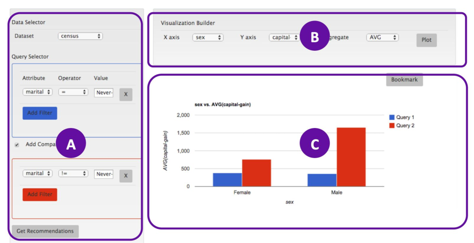
(a) Seedb [47]

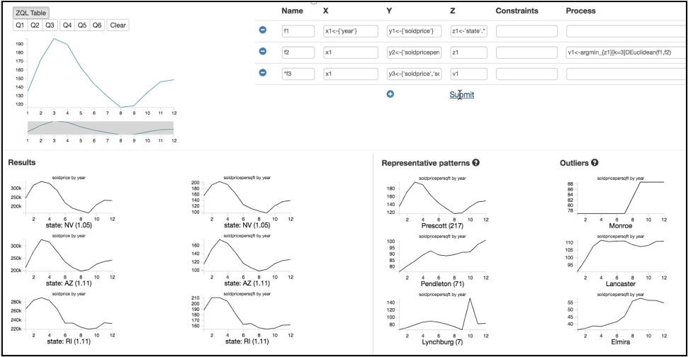
(b) Zenvisage [43]

Figure 1: Examples of comparative queries from visual analytic tools: a) Finding socio-economic indicators that differentiate married and unmarried couples in Seedb [47].The user specifies the subsets (A) after which the tool outputs a pair of attributes (B) along with corresponding visualizations (C) that differentiates the subsets the most. b) A comparative query in Zenvisage  [43] for finding states with comparable housing price trends.

The question we pose in this work is: can we efficiently perform comparison between subsets of data within the relational databases to improve performance and scalability of comparative queries? Supporting such queries within relational databases also makes them broadly accessible via general-purpose data analysis tools such as PowerBI [3], Tableau [5], and Jupyter notebooks [27]. All of these tools let users directly write SQL queries and execute them within the DBMS to reduce the amount of data that is shipped to the client.

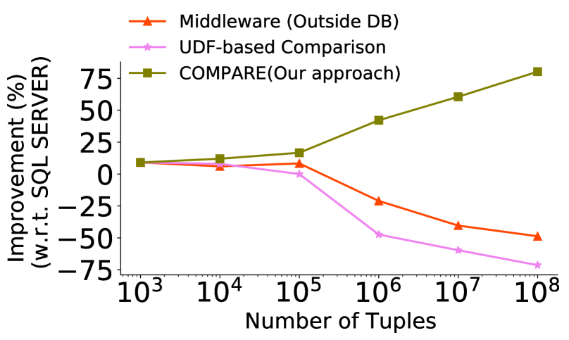
Figure 2: Relative performance of different execution approaches for a comparative query w.r.t unmodified SQL Server execution time (higher the better). The query finds a pair of origin airports that have the most similar departure delays over week trends in the flight dataset [1]

One option for in-database execution is to extend DBMS with custom user-defined functions (UDFs) for comparing subsets of data. However, UDFs incur invocation overhead and are executed as a batch of statements where each statement is run sequentially one after other with limited resources (e.g., parallelism, memory). As such, the performance of UDFs does not scale with the increase in the number of tuples (see Figure 2). Furthermore, UDFs have limited interoperability with other operators, and are less amenable to logical optimizations, e.g., PK-FK join optimizations over multiple tables.

While comparative queries can be expressed using regular SQL, such queries require complex combination of multiple subqueries. The complexity makes it hard for relational databases to find efficient physical plans, resulting in poor performance. While prior work have proposed extensions  [14, 13, 22, 18, 44] such as grouping variables, GROUPING SETs, CUBE; as we discussed in the later sections, expressing and optimizing grouping and comparison simultaneously remains a challenge. To describe the complexity using regular SQL, we use the following example.

Example. Consider a market analyst exploring sales trends across different cities. The analyst generates a sample of visualizations depicting different trends, e.g., average revenue over week, average profit over week, average revenue over country, etc., for a few cities. She notices that trends for cities in Europe look different from those in Asia. To verify whether this observation generalizes, she looks for a counterexample by searching for pairs of attributes over which two cities in Asia and Europe have most similar trends. Often, an $L_{p}$ norm-based distance measure (e.g., Euclidean distance, Manhattan distance) that measures deviation between trends and distributions is used for such comparisons [43, 47, 19].

Figure 3 depicts a SQL query template for the above example. The query involves multiple subqueries, one for each attribute pair. Within each subquery, subsets of data (one for each city) are aggregated and compared via a sequence of self-join and aggregation functions that compute the similarity (i.e., sum of squared differences). Finally, a join and filter is performed to output the tuples of subsets with minimum scores. Clearly, the query is quite verbose and complex, with redundant expressions across subqueries. While comparative queries often explore and compare a large number of attribute pairs [47, 28], we observe that even with only a few attribute pairs, the SQL specification can become extremely long.

Furthermore, the number of groups to compare can often be large—determined by the number of possible constraints (e.g., citi- es), pairs of attributes, and aggregation functions—which grow significantly with the increase in dataset size or number of attributes. This results in many subqueries with each subquery taking substantially long time to execute. In particular, while there are large opportunities for sharing computations (e.g., aggregations) across subqueries, the relational engines execute subqueries for each attrib- ute-pair separately resulting in substantial overhead in both runtime as well as storage. Furthermore, as depicted in subquery 1 in Figure 3, while each pair of groups (e.g., set of tuples corresponding to each city) can be compared independently, the relational engines perform an expensive self-join over a large relation consisting of all groups. The cost of doing this increases super-linearly as the number and size of subsets increases (discussed in more detail in Section 4.1). Finally, in many cases, we only need the aggregated result for each comparison; however the join results in large intermediate data—one tuple for each pair of matching tuples between the two sets, resulting in substantial overheads.

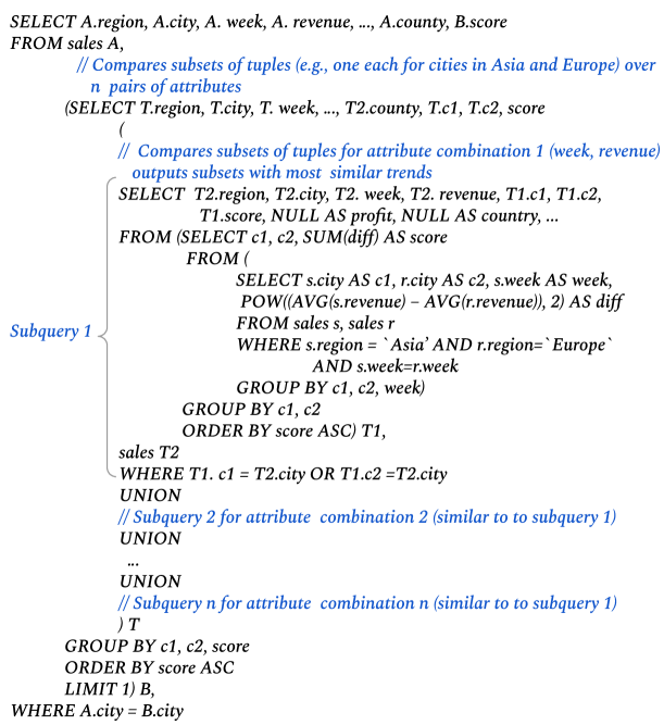
Figure 3: A SQL query for comparing subsets of data over different attribute combinations, depicting the complexity of specification using existing SQL expressions.

1.1 Overview of Our Approach

In this paper, we take an important step towards making specification of the comparative queries easier and ensuring their efficient processing. To do so, we introduce a logical operator and extensions to the SQL language, as well as optimizations in relational databases, described below.

Groupwise comparison as a first class construct (Section 2 and 3). We introduce a new logical operation, Compare ($\Phi$), as a first class relational construct, and formalize its semantics that help capture a large class of frequently used comparative queries. We propose extensions to SQL syntax that allows intuitive and more concise specification of comparative queries. For instance, the comparison between two sets of cities $C_{1}$ and $C_{2}$ over $n$ pairs of attributes: ($x_{1}$, $y_{1}$), ($x_{2}$, $y_{2}$), …, ($x_{n}$, $y_{n}$) using a comparison function $\mathcal{F}$ can be succinctly expressed as Compare [$C_{1}$<->$C_{2}$][ ($x_{1}$, $y_{1}$), ($x_{2}$, $y_{2}$), …, ($x_{n}$, $y_{n}$)] USING $\mathcal{F}$. As illustrated earlier, expressing the same query using existing SQL clauses requires a UNION over $n$ subqueries, one for each ($x_{i}$, $y_{i}$) where each subquery itself tends to be quite complex. Overall, while Compare does not give additional expressive power to the relational algebra, it reduces the complexity of specifying comparative queries and facilitates optimizations via query optimizer and the execution engine.

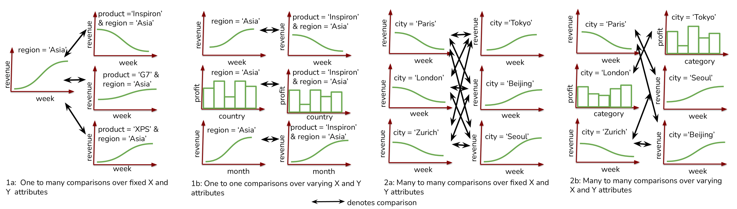
Figure 4: Illustrating comparative queries described in Section 2.1

Efficient processing via optimizations (Section 4 and 5). We exploit the semantics of Compare to share aggregate computations across multiple attribute combinations, as well as partition and compare subsets in a manner that significantly reduces the processing time. While these optimizations work for any comparison function, we also introduce specific optimizations (by introducing a new physical operator) that exploit properties of frequently used comparison functions (e.g., $L_{p}$ norms). These optimizations help prune many subset comparisons without affecting the correctness.

Inter-operator optimizations (Section 6). We introduce new transformation rules that transform the logical tree containing the Compare operator along with other relational operators into equivalent logical trees that are more efficient. For instance, the attributes referred in Compare may be spread across multiple tables, involving PK-FK joins between fact and dimension tables. To optimize such cases, we show how we can push Compare below join that reduces the number of tuples to join. Similarly, we describe how aggregates can be pushed below Compare, how multiple Compare operators can reordered and how we can detect and translate an equivalent sub-plan expressed using existing relational operators to Compare.

Implementation inside commercial database engine (Section 7). We have prototyped our techniques in Microsoft SQL Server engine, including the physical optimizations. Our experiments show that even over moderately-sized datasets (e.g., $10$–$20$ GB) Compare results in up to 4$\times$ improvement in performance relative to alternative approaches including physical plans generated by SQL Server, UDFs, and middlewares (e.g., Zenvisage, Seedb). With the increase in the number of tuples and attributes, the performance difference grows quickly, with Compare giving more than a order of magnitude better performance.

2 Characterizing Comparative
Queries

In this section, we first characterize comparative queries with the help of additional examples drawn from visualization tools [19, 43, 47] and data mining [35, 10, 8, 30]. Then, we give a formal definition that concisely captures the semantics of comparative queries.

2.1 Examples

We return to the example scenario discussed in introduction: a market analyst is exploring sales trends of products with the help of visualizations to find unusual patterns. The analyst first looks at a small sample of visualizations, e.g., average revenue over week trends for a few regions (e.g., Asia, Europe) and for a subset of cities and products within each region. She observes some unusual patterns and wants to quickly find additional visualizations that either support or disprove those patterns (without examining all possible visualizations). Note that we use the term "trend" to refer to a set of tuples in a more general sense where both categorical (e.g., country) or ordinal attributes (e.g., week) can be used for ordering or alignment during comparison. We consider several examples below in increasing order of complexity. Figure 4 illustrates each of these examples, depicting the differences in how the comparison is performed.

Example 1a. The analyst notes that the average revenue over week trends for Asia as well as for a subset of products in that region look similar. As a counterexample, she wants to find a product whose revenue over week trend in Asia is very dissimilar (typically measured using $L_{p}$ norms) to that of the Asia’s overall trend. There are visualization systems [48, 12, 43, 28] that support similar queries.

Example 1b. In the above example, the analyst finds that the trend for product ‘Inspiron’ is different from the overall trend for the region ‘Asia’. She finds it surprising and wants to see the attributes for which trends or distributions of Inspiron and Asia deviate the most. More precisely, she wants to compare ‘Inspiron’ and ‘Asia’ over multiple pairs of attributes (e.g., average profit over country, average quantitysold over week, …, average profit over week) and select the one where they deviate the most. Such comparisons can be found in features such as Explain Data[4] in Tableau and tools such as Seedb [47], Zenvisage [43], Voyager [49].

Example 2a. Consider another scenario: the analyst visualizes the revenue trends of a few cities in Asia and in Europe, and finds that while most cities in Asia have increasing revenue trends, those in Europe have decreasing trends. Again, as a counterexample to this, she wants to find a pair of cities in these regions where this pattern does not hold, i.e., they have the most similar trends. Such tasks involving search for similar pair of items are ubiquitous in data mining [36] and time series [35, 10, 8, 30].

Example 2b. In the above example, the analyst finds that the output pair of visualizations look different, supporting her intuition that perhaps no two cities in Europe and Asia have similar revenue over week trends. To verify whether this observation generalizes when compared over other attributes, she searches for pairs of attributes (similar to ones mentioned in Example 1b) for which two cities in Asia and Europe have most similar trends or distributions. Such queries are common in tools such as Zenvisage [43] that support finding outlier visualizations over a large set of attributes.

In summary, the comparative queries in above examples fast-forward the analyst to a few visualizations that depict a pattern she wants to verify—thereby allowing her to skip the tedious and time-consuming process of manual comparison of all possible visualizations. As illustrated in Figure 4, each query involves comparisons between two sets of visualizations (henceforth referred as Set1 and Set2) to find the ones which are similar or dissimilar. Each visualization depicting a trend is represented via two attributes (X attribute, e.g., week and a Y attribute, e.g., average revenue) and a set of tuples (specified via a constraint, e.g., product = ‘Inspiron’). We now present a succinct representation to capture these semantics.

2.2 Formalization

We formalize our notion of comparative queries and propose a concise representation for specifying such queries.

2.2.1 Trend

A trend is a set of tuples that are compared together as one unit. Formally,

Definition 1 (Trend).

Given a relation R, a trend $t$ is a set of tuples derived from R via the triplet: constraint $c$, grouping $g$, measure $m$ and represented as ($c$)($g$, $m$).

Definition 2 (Constraint).

Given a relation R, a constraint is a conjunctive filter of the form: $({p_{1}}=\alpha_{1},p_{2}=\alpha_{2},...,p_{n}=\alpha_{n})$ that selects a subset of tuples from R. Here, $p_{1},p_{2},...,p_{n}$ are attributes in $R$ and $\alpha_{i}$ is a value of $p_{i}$ in $R$. One can use ‘ALL’ to select all values of $p_{i}$, similar to [22].

Definition 3 ((Grouping, Measure)).

Given a set of tuples selected via a constraint, all tuples with the same value of grouping are aggregated using measure. A tuple in one trend is only compared with the tuple in another trend with the same value of grouping.

In example 1a, (R.region = ‘Asia’)(R.week, AVG(R.revenue)) is a trend in Set1, where (region = ‘Asia’) is a constraint for the trend and all tuples with the same value of grouping:‘week’ are aggregated using the measure: ‘AVG(revenue)’. We currently do not support range filters for constraint.

2.2.2 Trendset

A comparative query involves two sets of trends. We formalize this via trendset.

Definition 4 (Trendset).

A trendset is a set of trends. A trend in one trendset is compared with a trend in another trendset.

In example 1a, the first trendset consists of a single trend: {(R.region = ‘Asia’)(R.week, AVG(R.revenue))}, while the second trendset consists of as many trends as there are are unique products in $R$: {(R.region = ‘Asia’, R.product = ‘Inspiron’) (R.week, AVG(R.reven-ue)), (R.region = ‘Asia’, R.product = ‘XPS’)(R.week, AVG(R.reven- ue)), $...$, (R.region = ‘Asia’, R.product = ‘G7’) (R.week, AVG(R.rev- enue))}.

As is the case in the above example, often a trendset contains one trend for each unique value of an attribute (say $p$) as a constraint, all sharing the same (grouping, measure). Such a trendset can be succinctly represented using only the attribute name as constraint, i.e., [$p$][($g_{1}$, $m_{1}$)]. If $\alpha_{1}$, $\alpha_{2}$, ..$\alpha_{n}$ represent all unique values of $p$, then,

[$p$][($g_{1}$, $m_{1}$)] $\Rightarrow$ {($p=\alpha_{1}$)($g_{1}$, $m_{1}$), ($p=\alpha_{2}$)($g_{1}$, $m_{1}$), …, ($p=\alpha_{n}$)($g_{1}$, $m_{1}$)} ($\Rightarrow$ denotes equivalence)

Similarly, [$p_{1}$, $p_{2}=\beta$][($g_{1}$, $m_{1}$)] $\Rightarrow$ {($p_{1}=\alpha_{1}$, $p_{2}=\beta$)($g_{1}$, $m_{1}$), ($p_{1}=\alpha_{2}$, $p_{2}=\beta$)($g_{1}$, $m_{1}$), …, ($p_{1}=\alpha_{n}$, $p_{2}=\beta$)($g_{1}$, $m_{1}$)}

Alternatively, a trendset consisting of different (grouping, measure) combinations but the same constraint (e.g., $p=\alpha_{1}$) can be succinctly written as:

[($p=\alpha_{1}$)][($g_{1}$, $m_{1}$), …, ($g_{n}$, $m_{n}$)] $\Rightarrow$ {($p=\alpha_{1}$)($g_{1}$, $m_{1}$), …, ($p=\alpha_{1}$)($g_{n}$, $m_{n}$)}

2.2.3 Scoring

We first define our notion of ‘Comparability’ that tells when two trends can be compared.

Definition 5 (Comparability of two trends).

Two trends $t_{1}$: ($c_{1}$)($g_{1}$, $m_{1}$) and $t_{2}$: ($c_{1}$)($g_{2}$, $m_{2}$) can be compared if $g_{1}$ $=$ $g_{2}$ and $m_{1}$ $=$ $m_{2}$, i.e., they have the same grouping and measure.

For example, a trend (R.product = ‘Inspiron’) (R.week, AVG( R.revenue)) and a trend (R.product = ‘XPS’)( R.month, AVG(R.pro- fit)) cannot be compared since they differ on grouping and measure.

Next, we define a function scorer for comparing two trends.

Definition 6 (Scorer).

Given two trends $t_{1}$ and $t_{2}$, a scorer is any function that returns a single scalar value called ‘score’ measuring how $t_{1}$ compares with $t_{2}$.

While we can accept any function that satisfies the above definition as a scorer; as mentioned earlier, two trends are often compared using distance measures such as Euclidean distance, Manhattan distance [31, 47, 43]. Such functions are also called aggregated distance functions [34]. All aggregated distance functions use a function DIFF(.) as defined below.

Definition 7 (DIFF($m_{1},m2,p$)).

Given a tuple with measure value $m_{1}$ and grouping value $g_{i}$ in trend $t_{1}$ and another tuple with measure value $m_{2}$ and the same grouping value $g_{i}$, DIFF($m_{1}$, $m_{2}$, p) = $|m_{1}-m_{2}|^{p}$ where $p\in\mathbb{Z}^{+}$. Tuples with non-matching grouping values are ignored.

Since $m_{1}$ and $m_{2}$ are clear from the definition of $t_{1}$ and $t_{2}$ and tuples across trends are compared only when they have same grouping and measure expressions, we succinctly represent DIFF($m_{1}$, $m_{2}$, $p$) = DIFF($p$)

Definition 8 (Aggregated Distance Function).

An aggregated distance function compares trends $t_{1}:(c_{i})(g_{i},m_{i})$ and $t_{2}:(c_{j})$ $(g_{i},m_{i})$ in two steps: (i) first DIFF(p) is computed between every pairs of tuples in $t_{1}$ and $t_{2}$ with same values of $g_{i}$, and (ii) all values of DIFF(p) are aggregated using an aggregate function AGG such as SUM, AVG, MIN, and MAX to return a score. An aggregated distance function is represented as AGG OVER DIFF(p).

For example, $L_{p}$ norms such as Euclidean distance can be specified using SUM OVER DIFF(2), Manhattan distance using SUM OVER DIFF(1), Mean Absolute Deviation as AVG OVER DIFF(1), Mean Square Deviation as AVG OVER DIFF(2).

2.2.4 Comparison between Trendsets

We extend Definition 5 to the following observation over trendsets.

Observation 1 [Comparability between two trendsets] Given two trendsets $T_{1}$ and $T_{2}$, a trend $(c_{i})(g_{i},m_{i})$ in $T_{1}$ is compared with only those trends $(c_{j})(g_{j},m_{j})$ in $T_{2}$ where $g_{i}=g_{j}$ and $m_{i}=m_{j}$.

Thus, given two trendsets, we can automatically infer which trends between the two trendsets need to be compared. We use $T1$<->$T2$ to denote the comparison between two trendsets $T_{1}$ and $T_{2}$. For example, the comparison in example 1a can be represented as:

[region = ‘Inspiron’][(week, AVG(revenue))] <-> [region = ‘Asia’, product][ (week, AVG (revenue))]

If both $T_{1}$ and $T_{2}$ consist of the same set of grouping and measure expressions say {($g_{1}$, $m_{1}$), $...$, ($g_{n}$, $m_{n}$)} and differ only in constraint, we can succinctly represent $T_{1}$ <-> $T_{2}$ as follows:

[$c_{1}$][($g_{1}$, $m_{1}$), $...$, ($g_{n}$, $m_{n}$)] <-> [$c_{2}$][($g_{1}$, $m_{1}$), $...$, ($g_{n}$, $m_{n}$)] $\Rightarrow$ [$c_{1}$ <-> $c_{2}$][($g_{1}$, $m_{1}$), $...$, ($g_{n}$, $m_{n}$)]

Thus, the comparison between trendsets in example 1a can be succinctly expressed as:

[(region = ‘Asia’) <-> (region = ‘Asia’, product) ][(week, AVG(reve- nue))]

Similarly, the following expression represents the comparison in example 1b.

[(region = ‘Asia’) <-> (region = ‘Asia’, product = ‘Inspiron’)][(week,
AVG(revenue)), (country, AVG(profit)), … , (month, AVG(revenue))]

We can now define a comparative expression using the notions introduced so far.

Definition 9 (Comparative expression).

Given two trendsets $T_{1}$ <-> $T_{2}$ over a relation $R$, and a scorer $\mathcal{F}$, a comparative expression computes the scores between trends $(c_{i})(g_{i},m_{i})$ in $T_{1}$ and $(c_{j})$ $(g_{j},m_{j})$ in $T_{2}$ where $g_{i}=g_{j}$ and $m_{i}=m_{j}$.

3 The COMPARE Operator

In this section, we introduce a new operator Compare, that makes it easier for data analysts and application developers to express comparative queries. We first explain the syntax and semantics of Compare and then show how Compare inter-operates with other relational operators to express top-k comparative queries as discussed in Section 2.1.

3.1 Syntax and Semantics

Compare, denoted by $\Phi$, is a logical operator that takes as input a a comparative expression specifying two trendsets $T_{1}$ <->$T_{2}$ over relation $R$ along with a scorer $\mathcal{F}$ and returns a relation $R^{\prime}$.

$\Phi(R,T_{1}\text{{\color[rgb]{.75,.5,.25}\bf{<->}}}T_{2},\mathcal{F})$ $\rightarrow$ $R^{\prime}$

$R^{\prime}$ consists of scores for each pair of compared trends between the two trendsets. For instance, the table below depicts the output schema (with an example tuple) for the Compare expression [$c_{1}$ <-> $c_{2}$][($g_{1}$, $m_{1}$), ($g_{2}$, $m_{2}$)]. The values in the tuple indicate that the trend ($c1$ = $\alpha_{1}$)($g_{1}$, $m_{1}$) is compared with the trend ($c_{2}$ = $\alpha_{2}$)($g_{1}$, $m_{1}$) and the score is $10$.

$c_{1}$	$c_{2}$	$g_{1}$	$m_{1}$	$g_{2}$	$m_{2}$	score
$\alpha_{1}$	$\alpha_{2}$	True	True	False	False	$10$
…	…	…	…	…	…	…

We express the Compare operator in SQL using two extensions: Compare and USING:

⬇

COMPARE T1 <-> T2

USING $\mathcal{F}$

For instance, for example 1a, the comparison between the AVG(reve- nue) over week trends for the region ‘Asia’ and each of the products in region ’Asia’ can be succinctly expressed as follows:

Listing 1: COMPAREXPR1A

⬇

SELECT R1, P, W, V, score

FROM sales R

COMPARE [((R.region = Asia) AS R1) <-> (R1, R.product AS P)]

[R.week AS W, AVG (R.revenue) AS V]

USING SUM OVER DIFF(2) AS score

Table 1: Output of Compare in Example 1a

R1	P	W	V	score
Asia	XPS	True	True	30
Asia	Inspiron	True	True	24
…	…	…	…	…
Asia	G8	True	True	45

Here $T_{1}$ = [((R.region = Asia) AS R1)][R.week AS W, AVG (R.revenue) AS V] and $T_{2}$ = [((R.region = Asia) AS R1, R.product AS P)][R.week AS W, AVG (R.revenue) AS V]. Observe that $T_{1}$ and $T_{2}$ share the same set of (grouping, measure) and the filter predicate (R.region = Asia) in their constraints, thus it is concisely expressed as [((R.region = Asia) AS R1)<->(R1, R.product AS P)][R.week AS W, AVG (R.revenue) AS V].

Table 1 illustrate the output of this query. The first two columns R1 and P identify the values of constraint for compared trends in T1 and T2. The columns W and V are Boolean valued denoting whether R.week and AVG(R.revenue) were used for the compared trends. Thus, the values of (R1, P, W, V) together identify the pairs of trends that are compared. Since R.week and AVG(R.revenue) are grouping and measure for all trends in this example, their values are always True. Finally, the column score specifies the scores computed using Euclidean distance, expressed as SUM OVER DIFF(2).

Now, consider below the query for example 1b that compares tuples where (R.region = Asia) with tuples where (R.region = Asia) and (R.product = ’Inspiron’) over a set of (grouping, measure):

Listing 2: COMPAREXPR1B

⬇

SELECT R1, P, W, C, V, …, M, score

FROM sales R

COMPARE [((R.region = Asia) AS R1) <-> (R1, (R.product = ’Inspiron’)

AS P)][(R.week AS W, AVG(R.revenue) AS V), (R.country AS

C, AVG(R.profit) AS O), …, (R.month AS M, V)]

USING SUM OVER DIFF(2) AS score

Table 2: Output of Compare in Example 1b

R1	P	W	C	M	V	O	score
Asia	Inspiron	True	False	False	True	False	40
Asia	Inspiron	False	True	False	True	False	20
…	…	…	…	…	…	…	…
Asia	Inspiron	False	False	True	True	False	10

Table 2 depicts the output for this query. The columns R1 and P are always set to "Asia" and "Inspiron" since the constraint for all trends in T1 and T2 are fixed. W, C, M, V, and P consist of Boolean values telling which columns among R.week, R.country, R.month, AVG(R.revenue), and AVG(R.profit) were used as (grouping, measure) for the pair of compared trends.

From above examples, it is easy to see that we can write queries with Compare expression for examples 2a and 2b as follows:

Listing 3: COMPAREXPR2A

⬇

SELECT R1, C1, R2, C2, W, V, score

FROM sales R

COMPARE [((R.Region = Asia) AS R1, (R.city) AS C1) <-> ((R.Region

= Europe) AS R2, (R.city) AS C2)][R.week AS W,

AVG(R.revenue) AS V]

USING SUM OVER DIFF(2) AS score

Listing 4: COMPAREXPR2B

⬇

SELECT R1, C1, R2, C2, W, C, V, …, M, score

FROM sales R

COMPARE [((R.Region = Asia) AS R1, (R.city) AS C1) <-> ((R.Region

= Europe) AS R2, (R.city) AS C2)][(R.week AS W, AVG(R.revenue) AS

V), (R.country AS C, AVG(R.profit) AS O), …, (R.month AS M, V)]

USING SUM OVER DIFF(2) AS score

Note that Compare is semantically equivalent to a standard relational expression consisting of multiple sub-queries involving union, group-by, and join operators as illustrated in introduction. As such, Compare does not add to the expressiveness of relational algebra SQL language. The purpose of Compare is to provide a succinct and more intuitive mechanism to express a large class of frequently used comparative queries as shown above. For example, expressing the query in Listing 2 using existing SQL clauses (see Figure 3) is much more verbose, requiring a complex sub-query for each (grouping, measure). Prior work have proposed similar succinct abstractions such as GROUPING SETs [17] and CUBE [22] (both widely adopted by most of the databases) and more recently DIFF [6], which share our overall goal that with an extended syntax, complex analytic queries are easier to write and optimize.

Furthermore, the input to Compare is a relation, which can either be a base table or an output from another logical operator (e.g., join over multiple tables); similarly the output relation from Compare can be an input to another logical operator or the final output. Thus, Compare can interoperate with other operators. In order to illustrate this, we discuss how Compare interoperates with other operators such as join, filter to select top-k trends.

3.2 Expressing Top-k Comparative Queries

While Compare outputs the scores for each pair of compared trends, comparative queries often involve selection of top-$k$ trends based on their scores (Section 2.1). In this section, we show how we can use the above-listed Compare sub-expressions (referred by COMPAREXPR1A, COMPAREXPR1B, COMPAREXPR2A, and COMPAREXPR1B) with LIMIT and join to select tuples for trends belonging to top-$k$.

Example 1a. The following query selects the tuples of a product in region ‘Asia’ that has the most different AVG(revenue) over week trends compared to that of region ‘Asia’ overall. COMPAREXPR1A refers to the sub-expression in Listing 1.

⬇

SELECT T.product, T.week, T.revenue, S.score

FROM sales T JOIN

(SELECT * FROM COMPAREXPR1A

ORDER BY score DESC

LIMIT 1) AS S

WHERE T.product = S.P

The ORDER BY and LIMIT clause select the top-1 row in Table 1 with the highest score with P consisting of the most similar product. Next, a join is performed with the base table to select all tuples of the most similar product along with its score.

Example 2a. The query for example 2a differs from example 1a in that both trendsets consist of multiple trends. Here, one may be interested in selecting tuples of both cities that are similar, thus we use the WHERE condition (T.city = S.C1 AND T.Region = S.R1) OR (T.city = S.C2 AND T.Region = S.R2). (S.R1, S.R2, S.C1, S.C2) in SELECT clause identifies the pair of compared trends.

⬇

SELECT T.Region, T.city, T.week, T.revenue, S.R1, S.C1, S.R2, S.C2,

S.score

FROM sales T JOIN

(SELECT * FROM COMPAREXPR2A

ORDER BY score

LIMIT 1) AS S

WHERE (T.city = S.C1 AND T.Region = S.R1) OR (T.city = S.C2 AND

T.Region = S.R2)

Examples 1b and 2b. These examples extend the first two examples to multiple attributes. We show the query for example 2b; it’s a complex version of (example 1b) where trends in each trendsets are created by varying all three: constraint, grouping, measure (example 1b has a fixed constraint for each trendset).

⬇

SELECT T.city, S.R1, S.R2, S.C1, S.C2,

CASE WHEN S.W THEN T.week ELSE NULL END,

…

CASE WHEN S.V THEN T.revenue ELSE NULL END,

S.score

FROM sales T JOIN

(SELECT * FROM COMPAREXPR2B

ORDER BY score

LIMIT 1) AS S

WHERE (T.city = S.C1 AND T.Region = S.R1) OR (T.city = S.C2 AND

T.Region = S.R2)

The SELECT clause only outputs the values of columns for which corresponding trends has the highest score, setting NULL for other columns to indicate that those columns were not part of top-1 pair of trends. This idea of setting NULL is borrowed from prior work on CUBE [22]. Nevertheless, an alternative is to output values of all columns, and add (S.W, S.M, S.C, S.P, S.V) (as in the previous example) to the output to indicate which columns were part of the comparison between top-1 pair of trends.

4 Optimizing Comparative Queries

In this section, we discuss how we optimize a logical query plan consisting of a Compare operation. We extend the Microsoft SQL Server optimizer to replace Compare with a sub-plan of existing physical operators using two steps. First, we transform Compare into a sub-plan of existing logical operators. These logical operators are then transformed into physical operators using existing rules to compute the cost of Compare. The cost of the sub-plan for Compare is combined with costs of other physical operators to estimate the total cost of the query. We state our problem formally:

Problem 4.1.

Given a logical query plan consisting of Compare operation: $\Phi(R,$ [$c_{1}$<->$c_{2}$] [($d_{1}$, $m_{1}$), $...$, ($d_{n}$, $m_{n})]$, $\mathcal{F})$ $\rightarrow$ $R^{\prime}$, replace Compare with a sub-plan of physical operators with the lowest cost.

For ease of exposition, we assume that both trendsets contain the same set of trends, one for each unique value of $c$, i.e., $c_{1}$ = $c_{2}$ = $c$.

4.1 Basic Execution

We start with a simple approach that transforms Compare into a sub-plan of logical operators. The sub-plan is similar to the one generated by database engines when comparative queries are expressed using existing SQL clauses (discussed in Section 1). We perform the transformation using the following steps:

(1) $\forall(d_{i},m_{i})$: $R_{i}\leftarrow\text{Group-by}_{c,d_{i}}\text{Agg}_{m_{i}}(R)$

(2) $\forall$ $R_{i}$: $R_{ij}\leftarrow\Join_{R_{i}.c!=R_{i}.c,R_{i}.d_{i}=R_{i}.d_{i}}(R_{i})$

(3) $\forall$ $R_{ij}$: $R_{ijk}\leftarrow\text{Group-by}_{c^{i},c^{j}}\text{Agg}_{\text{UDA}_{\mathcal{F}}}(R_{ij})$ // $c^{i}$, $c^{j}$ are aliases of column $c$

(4) $R^{\prime}\leftarrow\underset{i,j,k}{\text{Union All}}(R_{ijk}$)

First, we create trendsets for each (grouping, measure) combination (e.g., GROUP BY product, week, AGG on AVG(reve- nue)). Next, we join tuples between each pair of trends that are compared, i.e., tuples with different constraints but same value of grouping (e.g., $\Join_{\text{R'.product !=\\ R'.product, R'.week = R'.week}})$). The score between each pair of trends is computed by applying $\mathcal{F}$ specified as an user-defined aggregate (UDA). This is done by first partitioning the join output to create a partition for each pair of trends. Each partition is then aggregated using $\mathcal{F}$. Finally, the scores from comparing each pairs of trends are aggregated via Union All.

Unfortunately, this approach has two issues that make it less efficient as the size of the input dataset and the number of (grouping, measure) combinations become large. First, aggregations across (grouping, measure) are performed separately, even when there are overlaps in the subset of tuples being aggregated. Second, the cost of join increases rapidly as the number of trends being compared and the size of each trend increases (see Figure 5(b)). We next discuss how we address these issues via merging and partitioning optimizations

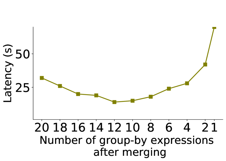
(a) Variation in performance as we merge group-by aggregates to share computations

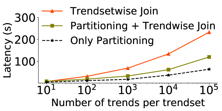
(b) Improvements due to trendwise join after partitioning trendset into trends (the size of each trend is fixed to 1000 tuples)

Figure 5: Improvement in performance due to merging group-by aggregates and trendwise comparison (via partitioning)

4.2 Merging and Partitioning Optimization

To generate a more efficient plan, we adapt the sub-plan generated above using two optimizations. We first describe each of these optimizations and then present an algorithm that incorporates both of these optimizations to find an overall efficient plan.

Merging group-by aggregates. The first optimization shares the computations across a set of group-by aggregates, one for each (grouping, measure), by merging them into fewer group-by aggregates. We observe that (grouping, measure) often share a common grouping column, e.g., [(day, AVG(revenue), (day, AVG(profit)] or have correlated grouping columns (e.g., [(day, AVG(revenue), (month, AVG(revenue)]) or have high degree of overlapping tuples across trends. For example, we considered a set of $20$ group-by aggregates in the flights [1] dataset, computing AVG(ArrivalDelay), AVG(DepDelay), …, AVG(Duration) grouped by day, week, …, airport. As depicted in Figure 5(a), by merging them (using an approach discussed shortly) into $12$ aggregates, the latency improves by 2$\times$. However, merging is helpful only up to a certain point, after which the performance degrades due to less sharing and much larger increase in the output size of group-by aggregates.

Finding the optimal merging of group-by aggregates is NP- Complete [7]. Prior work on optimizing GROUPING SETs computation [17] have proposed best-first greedy approaches that merge those group-by aggregates first that lead to maximum decrease in the cost. Unfortunately, in our setting, we also need to consider the impact of merging on the cost of subsequent comparison between trends; ignoring which can lead to sub-optimal plans as we describe shortly. We first introduce the second optimization for comparison.

Trendwise Comparison via Partitioning. The second optimization is based on the observation that pairwise joins of multiple smaller relations is much faster than the a single join between two large relations. This is because the cost of join increases super-linearly with the increase in the size of the trendsets. In addition to improvement in complexity, trendwise joins are more amenable to parallelization than a single join between two trendsets. Figure 5(b) depicts the difference in latency for these two approaches as we increase the number of trends from $10$ to $10^{5}$ (each of size $1000$). The black dotted line shows the partitioning overhead incurred while creating partitions for each trend, showing that the overhead is small (linear in $n$) compared to the gains due to trendwise join. Moreover, this is much smaller than the overhead incurred when partitioning is performed on the join output ($\propto$ $n^{2}$) in the basic plan (see step 3 in Section 4.1).

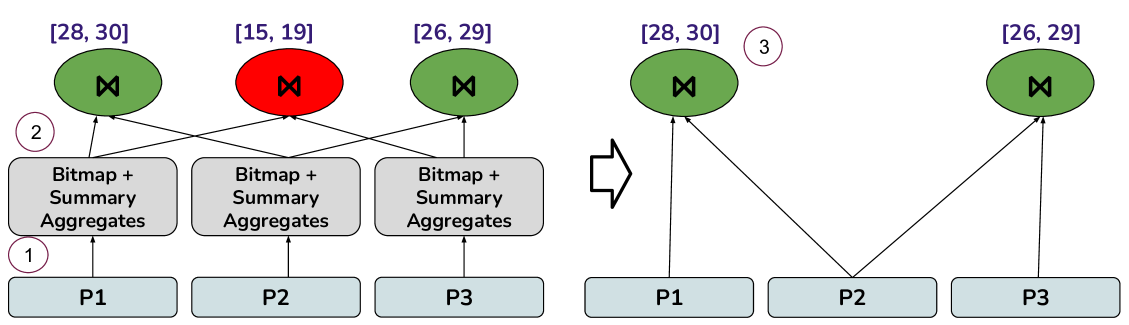
Figure 7: Illustrating pruning for DIFF-based comparisons

Figure 7 depicts the query plan after applying the above two optimizations on the basic query plan. First,we merge multiple group-by aggregates to share computations (using the approach discussed below). Then, we partition the output of merged group-by aggregates into smaller relations, one for each trend. This is followed by joining and scoring between each pair of trends independently and in parallel. Observe that the merging of group-by aggregates results in multiple trends with overlapping (grouping, measure) in the output relation. Hence, we apply the partitioning in two phases. In the first phase, we partition it vertically, creating one relation for each (grouping, measure). In the second phase, we partition horizontally, creating one relation for each trend.

Joint Optimization of Merging and Partitioning. As depicted in Figure 6b, the cost of partitioning increases with the increase in the size of its input. The input size is proportional to the number of unique group-by values, which increases with the increase in the number of merging of group-by aggregates. Thus, when the input becomes large, the cost of partitioning dominates the gains due to merging. It is therefore important to merge group-by aggregates such that the overall cost of computing group-by aggregates, partitioning and trendwise comparison together is minimal.

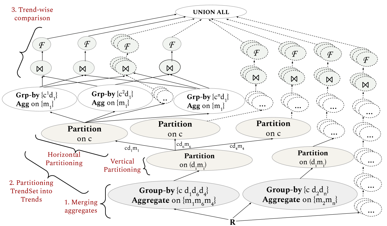
Figure 6: Optimized query plan generated after applying merging and partitioning on basic query plan in Figure 7.

In order to find the optimal merging and partitioning, we follow a greedy approach as outlined in Algorithm 1. Our key idea is to merge at the granularity of sub-plans instead of the group-by aggregates. We start with a set of sub-plans, one for each (grouping, measure) as generated by the basic execution strategy discussed earlier and merge two sub-plan at a time that lead to the maximum decrease in cost.

Formally, if the two sub-plans operate over ($d_{1}$, $m_{1}$) and ($d_{2}$, $m_{2}$) respectively, we merge them using the following steps (illustrated in Figure 6):

(1) $R1\leftarrow\text{Group-by}_{c,d_{1},d_{2}}\text{Agg}_{m_{2},m_{2}}[R]$ // merge group-by aggregates

(2) $\forall$ $(d_{i},m_{i})$: $R_{i}\leftarrow\Pi_{(d_{i},m_{i})}(R1)$ // vertical partitioning

(3) $\forall$ $i$: $R_{ij}\leftarrow\text{Partition }R_{i}\text{ ON }c$ // horizontal partitioning, one partition for each value of c

(4) $\forall$ $i,j$: $R_{i^{\prime}j^{\prime}}\leftarrow\text{Group-by}_{c_{j},d_{i}}\text{Agg}_{m_{i}}[R_{ij}]$ // aggregate again

(5) $\forall$ $i^{\prime},j^{\prime},k$: $R_{i^{\prime}j^{\prime}k}\leftarrow R_{i^{\prime}j^{\prime}}\Join_{d_{i}}R_{i^{\prime}k}$ //partitition-wise join

(6) $\forall$ $i^{\prime},j^{\prime},k$: $R^{{}^{\prime}}_{i^{\prime}j^{\prime}k}\leftarrow\text{Agg}_{\text{UDA}_{\mathcal{F}}}(R_{i^{\prime}j^{\prime}k})$ // compute scores

(7) $R^{\prime}\leftarrow\underset{i^{\prime},j^{\prime},k}{\text{Union All}}(R^{{}^{\prime}}_{i^{\prime}j^{\prime}k}$)

We first merge group-by aggregates to share the computation, followed by creating one partitions for each trend using both vertical and horizontal partitioning. Then, we join pairs of trends and compute the score as discussed in Section 4.1. For computing the cost of the merged sub-plan, we use the optimizer cost model. The cost is computed as a function of available database statistics (e.g., histograms, distinct value estimates), which also captures the effects of the physical design, e.g., indexes as well as degree of parallelism (DOP). We merge two sub plans at a time until there is no improvement in cost.

Algorithm 1 Merge-Partition Algorithm

1:Let $B$ be a basic sub-plan computed from $\Phi$ as described in Section 4.1

2:while true do

3:    $C$ $\leftarrow$ OptimizerCost(B)

4:    Let $s_{i}$ $\in$ $S$ be a sub-plan in B consisting of a sequence of group-by aggregate, join and partition operations over ($d_{i}$, $m_{i}$)

5:    Let $MP$ = Set of all sub-plans obtained by merging a pair of sub-plans in $S$ as described in Section 4.2

6:    Let $B_{new}$ be the sub-plan in $MP$ with lowest cost ($C_{new}$) after merging two sub-plans $s_{i},s_{j}$

7:    if $C_{new}>C$ then

8:         break;

9:    end if

10:    $C$ $\leftarrow$ $C_{new}$

11:    $B$ $\leftarrow$ $B_{new}$

12:end while

13:Return B

5 Optimizing DIFF-based Comparison

While the approach discussed in the previous section works for any arbitrary scorer (implemented as UDA), we note that for top-$k$ comparative queries involving aggregated distance functions (defined in Section 2.2) such as Euclidean distance, we can substantially reduce the cost of comparison between pairs of trends. We first outline the three properties of DIFF(.) function that we leverage for optimizations.

1. Non-negativity: DIFF( $m_{1},m_{2},p$) $\geq 0$

2. Monotonicity: DIFF($m_{1},m_{2},p$) varies monotonically with the increase or decrease in $|m_{1}-m_{2}|$.

3. Convexity: DIFF( $m_{1},m_{2},p$) are convex for all $p$.

5.1 Summarize $\rightarrow$ Bound $\rightarrow$ Prune

Overview. We introduce a new physical operator that minimizes the number of trends that are compared using the following three steps (illustrated in Figure 8). 1. We summarize each trend independently using a set of three aggregates: SUM, MIN and MAX and a bitmap corresponding to the grouping column. 2. Next, we intersect the bitmaps between trends to compute the COUNT of matching tuples between trends, which together with three aggregates help compute the upper and lower bounds on the score between the two trends. Given bounds on scores for each pair of trends, we find a pruning threshold T on the lowest possible top $k$ score, as the $k$th largest lower bound score. Any pair with its upper bound score smaller than T can thus be pruned. 3. Finally, we perform join only between those trends that are not pruned.

Figure 8: Using summaries to bound scores. $\mathcal{F}$ = SUM OVER DIFF($2$). Each value in (a) corresponds to a single tuple in a trend.

While the pruning incurs an overhead of first computing the summary aggregates and bitmap for each candidate trend, the gains from skipping tuple comparisons for pruned trends offsets the overhead. Moreover, the summary aggregates of each trend can be computed independently in parallel.

Computing Bounds. The simplest approach is to create a single set of summary aggregates for each trend as depicted in Figure 8b. The gray and yellow blocks depict the summary aggregates for two trends respectively, consisting of COUNT (computed using bitmaps), SUM, MIN, and MAX in order.

First, for deriving the lower bound, we prove the following useful property based on the convexity property of DIFF functions (see  [2] for the proof).

Theorem 1. $\forall$ DIFF$(m_{1},m_{2},p)$,
          AVG (DIFF$(m_{1},m_{2},p))\geq$ DIFF(AVG $(m_{1})$,AVG $(m_{2}),p)$

This essentially allows us to apply DIFF on the average values of each trend to get a sufficiently tight lower bounds on scores. For example, in Figure 8b, we get a lower bound of $1700$ for a score of $1717$ for the two trends shown in Figure 8b.

For the upper bound, it is easy to see that the maximum value of DIFF($m_{1}$, $m_{2}$, 2) between any pairs of tuples in R and S is given by: MAX ( |MAX ($m_{1}$) $-$ MIN ($m_{2}$)|, |MAX ($m_{2}$) $-$ MIN ($m_{1}$)|). Given that DIFF($m_{1},m_{2},2$) is Non-negative and Monotonic, we can compute the upper bound on SUM by multiplying the the MAX (DIFF($m_{1},m_{2},2$)) by COUNT. For example, in Figure 8b, we get an upper bound of $6400$.

Multiple Piecewise Summaries. Given that the value of measure can vary over a wide range in each trend, using a single summary aggregate often does not result in tight upper bound. Thus, to tighten the upper bound, we create multiple summary aggregates for each trend, by logically dividing each trend into a sequence of $l$ segments, where segment $i$ represents tuples from index: $(i-1)\times\frac{n}{l}+1$ to $i\times\frac{n}{l}$ where $n$ is the number of tuples in the trend. Instead of creating a single summary, we compute a set of same summary aggregates over each segment, called segment aggregates. For example, Figure 8c depicts two segment aggregates for each trend, with each segment representing a range of $8$ tuples. The bounds between a pair of matching segments is computed in the same way as we described above for a single summary aggregates. Then, we sum over the bounds across all pairs of matching segments to get the overall bound (see  [2] for formal description). To estimate the number of summary aggregates for each trend, we use Sturges formula, i.e., ($\left\lfloor 1+log_{2}(n)\right\rfloor$) [42], which assumes the normal distribution of measure values for each trend. Because of its low computation overhead and effectiveness in capturing the distribution or trends of values, Sturges formula is widely used in the statistical packages for automatically segmenting or binning data points into fewer groups. We empirically evaluate the effectiveness of Sturges formula in Section 8.

5.2 Early Termination

When selecting top-$k$ trends, we can further reduce the computation by ordering the comparison of trends that are not pruned in the previous step. To do so, we assign an utility to each of the trends that tells how likely they are going to be in the top-$k$. For estimating the utility of trends, we use the bounds computed using segment aggregates. Specifically, for selecting top-$k$ trends in descending order of their scores, a trend with higher upper bound score has a higher utility and for ascending order of scores, a trend with the smallest lower bound has a higher utility. The processing of higher utility trends leads to the faster improvement in the pruning threshold, thereby minimizing wastage of tuple comparisons over low utility trends.

Furthermore, the utility of a trend can vary after comparing a few tuples in a candidate trend. Hence, instead of processing the entire trend in one go, we process one segment of a trend at a time, and then update the bounds to check (i) if the trend can be pruned, or (ii) if there is another trend with better utility that we can switch to. Incrementally comparing high utility trends leads to pruning of many trends without processing all of their tuples.

5.3 Putting It All Together

We implemented a new physical operator, $\Phi_{p}$, that takes as input the trends, and replaces the join and $\mathcal{F}$ in query plan discussed in Section 4. It outputs a relation consisting of tuples that identify the top-$k$ pairs of trends along with their scores. The algorithm used by the operator makes use of four data structures: (1) SegAgg : An array where index $i$ stores summary aggregates for segment $i$. There is one SegAgg per trend. (2) TState : It consists of the current upper and lowers bounds on the score between two trends, as well as the next segment within the trends to be compared next. There is one TState for each pairs of trends, and is updated after comparing each pairs of segment. (3) $\mathcal{PQ}_{\mathcal{P}}$: a max priority queue that keeps track of the trend pairs with the highest upper bound. It is updated after comparing each segment. (4) $\mathcal{PQ}_{\mathcal{S}}$: a min priority queue that keeps track of the trend pairs with the smallest lowest bound. It is updated after comparing each segment.

Algorithm 2 Pruning Algorithm for DIFF-based Comparison

1:Compute SegAgg and bitmaps for each trend $c_{i}$

2:for each pair of trends $c_{i}$, $c_{j}$ do

3:    Compute bounds on scores (Section 5.1)

4:    Update $\mathcal{PQ}_{\mathcal{S}}$

5:end for

6:for each pair of trends $(c_{i},c_{j})$ do

7:    If ($(c_{i},c_{j})$ upper bound $<$ $\mathcal{PQ}_{\mathcal{S}}$.Top()) Continue;

8:    Initialize $(c_{i},c_{j})$ TState and push to $\mathcal{PQ}_{\mathcal{P}}$

9:end for

10:while size of $\mathcal{PQ}_{\mathcal{P}}$ $>$ $k$  do

11:    $(c_{i},c_{j})=$ $\mathcal{PQ}_{\mathcal{P}}$.Top()

12:    Compare a segment of $c_{i}$ with that of $c_{j}$

13:    Update bounds and $\mathcal{PQ}_{\mathcal{S}}$

14:    If ($(c_{i},c_{j})$ upper bound $<$ $\mathcal{PQ}_{\mathcal{S}}$.Top()) Continue;

15:    Push $(c_{i},c_{j})$ to $\mathcal{PQ}_{\mathcal{P}}$

16:end while

17:Return Top $k$ trend pairs of trends and their scores from $\mathcal{PQ}_{\mathcal{P}}$

Algorithm 2 depicts the pseudo-code for a single threaded implementation. We first compute the segment aggregates for trends (line $1$). For each pair of trends, we compute the bounds on scores as discussed in Section 5.1, and update $\mathcal{PQ}_{\mathcal{S}}$ to keep track of top $k$ lower bounds (lines $2$—$5$). The upper bound for each pair of trend is compared with $\mathcal{PQ}_{\mathcal{S}}$.Top() to check if it can be pruned (line $7$). If not pruned, the TState is initialized and pushed to $\mathcal{PQ}_{\mathcal{P}}$ (line $8$). Once the TState of all unpruned trends are pushed to $\mathcal{PQ}_{\mathcal{P}}$, we fetch the pair of trends with the highest upper bound score ((line $11$)), and following the process outlined in Section 5.2, compare a pair of segments (line $12$). After the comparison, we check if the current pair of trends is pruned or if there is another pair of trends with higher upper bound (line $14$–$15$). This process is continued until we are left with $k$ pairs of trends . Finally, we output values of $k$ pairs of trends with highest scores (line $17$).

Memory Overhead. Given a relation of $n$ tuples consisting of $p$ trends, $\Phi_{p}$ creates $p\times log(n/p)$ segment aggregates (assuming tuples are uniformly distributed across trends), with each segment aggregate consisting of fixed set of aggregates. In addition, the operator maintains a TState consisting of bounds on scores between each pair of trends as well as the priority queues to maintain top-k pairs of trends. Thus, the overall space overhead is $O(p\times log(n/p)+p^{2})$.

6 Additional Algebraic Rules

The query optimizer in Microsoft SQL Server relies on algebraic equivalence rules for enumerating query plans to find the plan with the least cost. When Compare occurs with other logical operators, we present five transformation rules (see Table LABEL:tab:equivrules) that reorder $\Phi$ with other operators to generate more efficient plans.

R1. Pushing $\Phi$ below join. Data warehouses often have a snowflake or star schema, where the input to Compare operation may involve a PK-FK join between fact and dimension tables. If one or more columns in $\Phi$ are the PK columns or have functional dependencies on the PK columns in the dimension tables , $\Phi$ can be pushed down below the join on fact table by replacing the dimension tables columns with the corresponding FK columns in the fact table (see Rule $R_{1}$ in Table LABEL:tab:equivrules.) For instance, consider example 1a in Section 2.1 that finds a product with a similar average revenue over week trend to ‘Asia’. Here, revenue column would typically be in a fact table along with foreign key columns for region, product and year. In such cases, we can push $\Phi$ below the join by replacing dimension table columns (e.g., product, week) values with corresponding PK column values.

R2. Pushing Group-by Aggregate ($\Upsilon$) below $\Phi$ to remove duplicates. When an aggregate operation occurs above a Compare operation, in some cases we can push the aggregate operation below the Compare to reduce the size of each partition. In particular, consider an aggregate operation $\Upsilon_{G,A}$ with group by attributes $G$ and aggregate function $A$ such that all columns used in $\Phi$ are in $G$. Then, if all aggregation functions in $\Phi$ $\in$ {MAX, MIN }, we can push $\Upsilon$ below $\Phi$ as per the Rule $R_{2}$ in Table LABEL:tab:equivrules. Pushing aggregation operation below $\Phi$ reduces the size of each partition by removing the duplicate values.

R3. Predicate pushdown. A filter operation ($\sigma$) on partition column (e.g., product) can be pushed down below $\Phi$, to reduce the number of partitions to be compared. While predicate pushdown in a standard optimization, we notice that optimizers are unable to apply such optimizations when the Compare are expressed via complex combination of operations as described in Section 1. Adding an explicit logical Compare, with a predicate pushdown rule makes it easier for the optimizer to apply this optimization. Note that if $\sigma$ involves any attribute other than the partitioning column, then we cannot push it below $\Phi$. This is because the number of tuples for partitions compared in $\Phi$ can vary depending on its location.

R4. Commutativity. Finally, a single query can consist of a chain of multiple Compare operations for performing comparison based on different metrics (e.g., comparing products first on revenue, and then on profit). When multiple $\Phi$ operations on the same partitioning attribute, we can swap the order such that more selective Compare operation is executed first.

R5. Reducing comparative sub-plans to $\Phi$. Finally, we extend the optimizer to check for an occurrence of the comparative sub-expression specified using existing relational operators to create an alternative candidate plan by replacing the sub-expression with $\Phi$. In order to do so, we add the equivalence rule R5 where the expression on the left side represents the sub-expression using existing relational operators. This rule allows us to leverage physical optimizations for comparative queries expressed without using SQL extensions.

7 Discussion

We discuss the generalizability and robustness of our proposed optimizations as well as potential applications of Compare.

Generalizability of optimizations. Our proposed optimizations in Section 4 deal with replacing Compare to a sub-plan of logical and physical operators within existing database engines. These optimizations can be incorporated in other database engines supporting cost-based optimizations and addition of new transformation rules. Concretely, given a Compare expression, one can generate a sub-plan using Algorithm 1 and transformation rules implementing steps outlined in Section 4.1 and Section 4.2. Furthermore, we discuss additional transformation rules (see Table 3) in Section 6 that optimize the query when Compare occurs along with other logical operators such as join, group-by, and filter. We show that DIFF-based comparisons can be further optimized by adding a new physical operator that first computes the upper and lower bounds on the scores of each trend, which can then be used for pruning partitions without performing costly join.

Robustness to physical design changes. A large part of Compare execution involves operators such as group-by, joins and partition (See Figure 6). Hence, the effect of physical design changes on Compare is similar to their effect on these operators. For instance, since column-stores tend to improve the performance of group-by operations, they will likely improve the performance of Compare. Similarly, if indexes are ordered on the columns used in constraints or grouping, the optimizer will pick merge join over hash-join for joining tuples from two trends. Finally, if there is a materialized view for a part of the Compare expression, modern day optimizers can match and replace the part of the sub-plan with a scan over the materialized view. We empirically evaluate the impact of indexes on Compare implementation in Section 8.

Applications of Compare. Compare is meant to be used by data analysts as well as applications to issue comparative queries over large datasets stored in relational databases. It has two advantages over regular SQL and middleware approaches (e.g., Zenvisage, Seedb). First, it allows succinct specification of comparative queries which can be invoked from data analytic tools supporting SQL clients. Second, it helps avoid data movement and serialization and deserialization overheads, and is thus more efficient and scalable. We classify the applications into three categories:

BI Tools. BI applications such as Tableau and Power BI do not provide an easier mechanism for analysts to compare visualizations. However, for supporting complex analytics involving multiple joins and sub-queries, these tools support SQL querying interfaces. For comparative queries, users currently have to either write complex SQL queries as discussed in Introduction, or generate all possible visualizations and compare them manually. With Compare, users can now succinctly express such queries (as illustrated in Section 3) for in-database comparison.

Notebooks. For large datasets stored in relational databases, it is inefficient to pull the data into notebook and use dataframe APIs for processing. Hence, analysts often use a SQL interface to access and manipulate data within databases. While one can also expose Python APIs for comparative queries and automatically translate them to SQL, such features are limited to the users of the Python library. SQL extensions, on the other hand, can be invoked from multiple applications and languages that support SQL clients. Furthermore, in the same query, one can use Compare along with other relational operators such as join and group-by that are frequently used in data analytics (see Section 3.2).

Visual analytic tools. Finally, there are visual analytic tools such as as Zenvisage and Seedb that perform comparison between subsets of data in a middle-ware. With Compare, such tools can scale to large datasets and decrease the latency of queries as we show in Section 8.

Table 3: Queries over Flight and TPC-DS datasets

ID	1cmType	Flight						TPC-DS
		trendset 1			trendset 2			trendset 1			trendset 2
		constraint, #	(grouping,measure), #	# trends	constraint, #	(grouping,measure), #	# trends	constraint, #	(grouping,measure), #	# trends	constraint, #	(grouping,measure), #	# trends
Q1	One to many with fixed attributes	airport=‘SFO’, 1	(Days, ArrDelays), 1	1	all airports, 384	(Days, ArrDelays)	384	webpage = 1; 1	(Items, NetProfits), 1	1	all webpages; 2040	1	2040
Q2	Many to many with fixed attributes	all airports, 384	(Days, ArrDelays), 1	384	all airports, 384	(Days, ArrDelays)	384	all webpages; 2040	(Items, NetProfits), 1	2040	all webpages; 2040	(Items,NetProfits), 1	2040
Q3	One to one with varying attributes	airport=‘SFO’, 1	(Days, ArrDelays), (Days, DepDelays), (Weeks, ArrDelays), …, (Weeks, WeatherDelays,); 10	10	airport = ‘SFO’, 1	(Days, ArrDelays), (Days, DepDelays)), (Weeks, ArrDelays), …, (Weeks, DepDelays); 10	10	webpage = 1; 1	(Items, NetProfits), (Days, NetProfits), …, (Days, Quantity),5	5	webpage = 1; 1	(Items, NetProfits), (Days, NetProfits), …, (Days, Quantity),5	5
Q4	Many to many with varying attribues	all airports, 384	(Days, ArrDelays), (Days, DepDelays), (Weeks, ArrDelays), …, (Weeks, WeatherDelays,); 10	3840	all airports	(Days, ArrDelays), (Days, DepDelays), (Weeks, ArrDelays), …, (Weeks, WeatherDelays,); 10	3840	all webpages; 2040	(Items, NetProfits), (Days, NetProfits), …, (Days, Quantity),5	10200	all webpages; 2040	(Items, NetProfits), (Days, NetProfits), …, (Days, Quantity),5	10200

8 Performance Evaluation

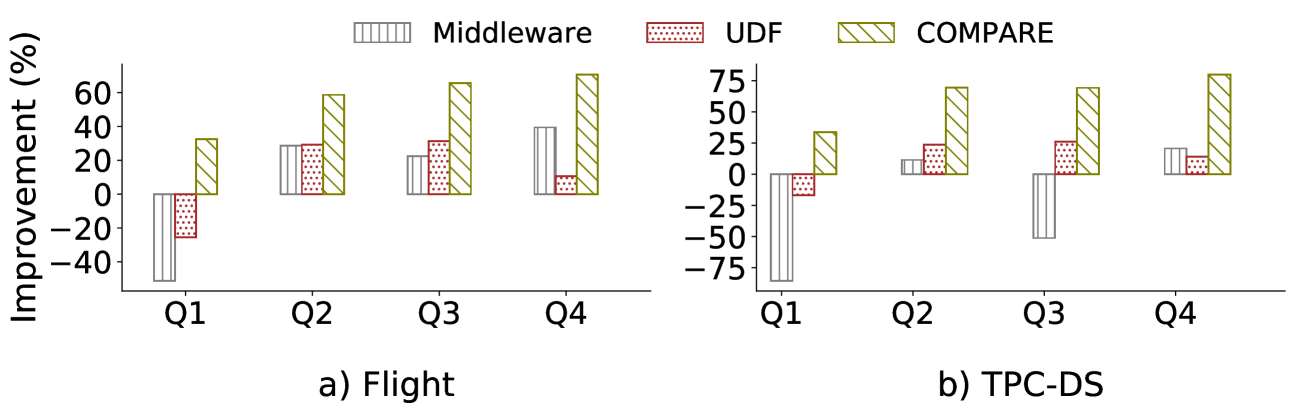
(a) Comparison with Baselines

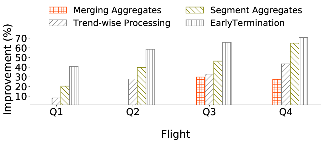
(b) Ablative analysis quantifying the impact of each optimization. Each optimization is successively turned on from left to right.

Figure 9: Improvement in end-to-end latency w.r.t. unmodified SQL Server

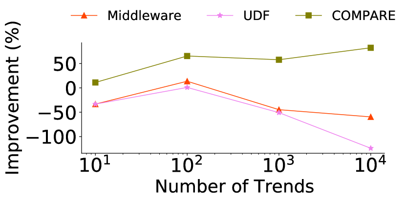
(a) Varying number of trends with fixed (grouping, measure)

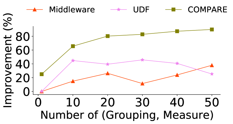
(b) Varying number of (grouping, measure)

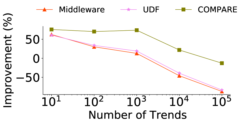
(c) Increasing number of trends with proportional decrease in trend size over a fixed data of size $10^{5}$

Figure 10: Impact on latency on varying the number and size of trends on the flight dataset.

Using our prototype implementation on SQL Server (referred as Compare below), we evaluate the improvement in latency with respect to current execution strategy in SQL Server as described in Section 4.1. We consider two alternative strategies as baselines: (b) Middleware: Issuing select-aggregate queries to retrieve the data from SQL Server over a network (average speed of 10 MB/s) and performing comparison and filtering in a C# implementation; this approach mimics the data retrieval approach followed by visualization tools such as Zenvisage [43] while also incorporating trendwise comparison and segment-aggregates based pruning optimizations (discussed in Section 5), and (c) an UDF implementation that executes within SQL Server. It takes as input the UNION of all group-by aggregates (computed via GROUPING SETs clause) and incorporates trendwise comparison and segment-aggregates based pruning optimizations.

Datasets and Queries. We use two datasets: Flight [1] and TPC-DS with a scale factor of $100$ [32](summarized in Table 4). We use websales table in TPC-DS which has PK-FK joins with tables webpages and warehouses. As depicted in Table 3, we issue four types of comparative queries (with characteristics similar to examples discussed in Section 2.1), with the default number of output pair of trends set to $5$. All measure attributes are aggregated using AVG() and we use SUM() OVER DIFF(2) as scorer.

Table 4: Datasets

Dataset	Disk Size	Buffer Size	Number of rows
Flight	8GB	11GB	74M
TPC-DS	20GB	24 GB	720M

Setup. All experiments were conducted on a 64-bit Windows 2012 Server with 2.6GHz Intel $\times$eon E3-1240 10-core, 20 logical processors and 192GB of 2597 MHz DDR3 main memory. Unless specified, we use the default settings for the degree of parallelism (DOP) and buffer memory, where the SQL Server tries to utilize the maximum possible resources available in the system. We report the results of warm runs by loading the tables referenced in the query into memory.

8.1 End-to-End Latency

Figure 9(a) depicts the end-to-end improvement in latency of Compare, Middleware, and UDF with respect to the unmodified SQL Server runtimes. We see that Compare provides a substantial improvement with respect to all approaches, with improvement being proportional number and size of trends.

For Q1 that involves one to many comparisons over a fixed attribute combination, we see a speed-up of about 26% on Flight and about 36% on the TPC-DS. The improvement increases substantially as we increase the complexity of the query; for example we see upto 4$\times$ improvement in latency for Q2 and Q4 which involve a large number of trend comparisons. For Middleware, the main bottleneck is the data transfer and deserialization overhead, which takes up to $70\%$ of the overall execution time. While UDF also incurs an overhead in invocation and reading the input from downstream aggregate operators, a large part of its time ( $>$ 90%) is spent on processing, indicating that inline execution of Compare via partitioning and join operators is much faster. In summary, we find that Compare gives the best of both worlds: requires minimal data transfer and deserialization overhead, and runs much faster by efficiently comparing tuples within databases.

Ablative Analysis. Next, we conducted an ablative analysis to evaluate the effectiveness of each of the optimizations described in Section 4 and Section 5. Figure 9(b) depicts the impact of each optimization as we add them successively from left to right. Each level of Compare optimization provides a substantial speed-up in latency compared to basic execution strategy. For Q3 and Q4, sharing aggregates improves the runtime by about 30% (note that there are no sharing opportunities for Q1 and Q2). The trend-wise processing further improves the processing by 25% on average—more the number of trend comparisons, the higher the improvement. Note that both sharing aggregates and trend-wise processing do not depend on the properties of scorer and hence can be applied on arbitrary scorer. The next two optimizations based on segment-aggregates and early termination, although only applicable for DIFF($m_{1},m_{2},2$)-based comparison, result in the massive improvement ranging between 20-25% by pruning trends early that are guaranteed to be not in top-k.

8.2 Sensitivity to Data Characteristics

We now evaluate the impact of dataset characteristics on the performance of Compare. For these experiments, we use the flight dataset (consisting of real-world trends/distributions) and scale its size as described below.

Impact of number of trends. To evaluate this, we scale the number of trends for query Q2 between $10$ and $10^{4}$ by randomly removing or replicating the trends corresponding to original $384$ airports. While replicating, we update the original value $m_{o}$ of each measure column $m$ by a new value $m_{n}$ where $m_{n}$ = $m_{o}$ ± $stdev(m)$. This ensures that the replicated trends are not duplicates but still represent the original distribution. We find that the increase in the number of trends leads to the increase in latency for all approaches; however the increase is much higher for UDF and Middleware due to data movement and deserialization overhead. Compare is further able to reduce comparisons due to early pruning of partitions using segment-aggregates.

Impact of number of (grouping, measure). In this case, we scale the number of (grouping, measure) for query Q3 between $1$ and $50$ by randomly removing or replicating the columns for each trend while updating the values of replicated measure column as described above. All approaches incur increase in latency; however, the increase in latency is much higher for SQL Server compared to Compare, Middleware and UDF due to higher sharing of aggregate computations.

Varying number and size of trends while keeping the overall data size fixed. Using a similar process as described above, we scale the number of trends between $10$ and $10^{5}$ while proportionally decreasing the size of each trend such that the size of the dataset is fixed to $10^{5}$. Here, we see an interesting observation. The latency of SQL Server decreases as we increase the number of trends and reduce their size. This is because with the decrease in the size of trends, the number of tuple comparison decreases. As a result of this, the improvement in latency w.r.t SQL Server decreases for all of Compare, Middleware, and UDF. However, for Compare, the latency initially decreases as sorting and comparison can done faster in parallel as the number of partitions increase. As the number of partitions become too large, the improvement due to parallelism decreases.

8.3 Impact of Number of Segment Aggregates

Recall from Section 5.1 that we use the Sturges formula [42], i.e., ($\left\lfloor 1+log_{2}(n)\right\rfloor$) (where $n$ is the estimated size of trend) to estimate the number of segment-aggregates. To measure the efficacy of this formula, we measure the changes in latency as we increase the number of segment-aggregates for Q2 (Figure 11(a)) and Q4 (Figure 11(b)). With the increase in number of segments, the overall latency decreased initially. However, as the number of segments is increased beyond a certain number, the latency starts increasing. This is because of the increase in the number of segment-aggregates comparisons without further pruning. The dotted line shows the results for the number of segments (i.e., ($\left\lfloor 1+log_{2}(n)\right\rfloor$) that is automatically selected by Compare, showing that the latency for selected segments is close to minimal possible latency.

Next, we measure the impact of number of tuples processed per update for early termination (Section 5.2). Figure 12 depicts the impact of overall latency for $Q2$ and $Q_{4}$ as we vary the number of tuples processed for a given trend for updating the upper and lower bounds. The dotted black line depicts the performance for the number of tuples that Compare automatically decides, i.e., ($\frac{n}{(\left\lfloor 1+log_{2}(n)\right\rfloor)}$) (i.e., estimated size of a segment). We see that the latency is very high when we only consider a few tuples ($<10$) at time. This is because of cache misses and many updates to the priority queues for reprocessing the same set of partitions repeatedly. On the other hand, processing too many tuples leads to extra processing, even for low utility partitions that can be pruned earlier. As depicted by the dotted line, the number chosen by Compare, although not perfect, is close to the optimal performance that we can get by processing few tuples at a time.

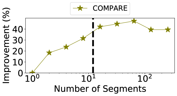
(a) $Q_{2}$

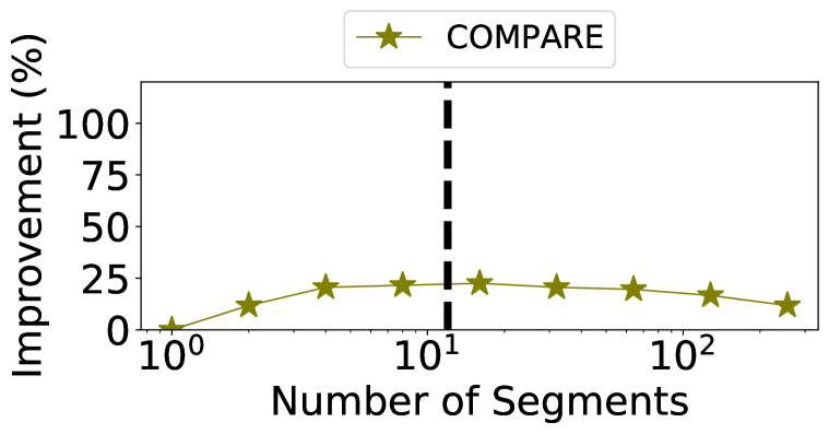
(b) $Q_{4}$

Figure 11: Varying number of segment-aggregates

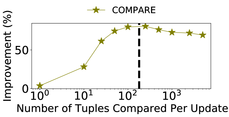
(a) $Q_{2}$

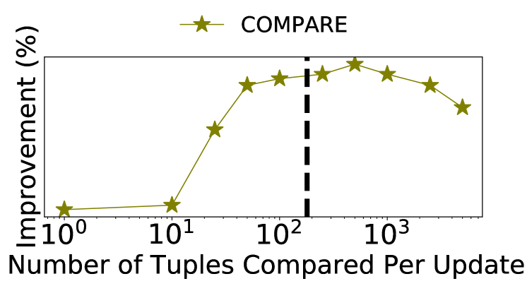
(b) $Q_{4}$

Figure 12: Varying number of tuples compared per update during early termination

8.4 Impact of Transformation Rules

Figure 13 depicts the performance results on pushing $\Phi$ below PK-FK joins ($\Join$) and pushing Aggregate ($\Upsilon$) below $\Phi$. We omit the results on other logical optimizations such as predicate pushdown and reordering of multiple $\Phi$ operations as the gains in these cases are always proportional to the selectivity of predicates and $\Phi$ operation pushed down.

Pushing $\Phi$ below $\Join$. We consider $Q_{3}$ and $Q_{4}$ over websales table of TPC-DS dataset which has PK-FK joins with two other tables. We observe that by pushing $\Phi$ below join leads to the improvement in the runtime of both queries due to reduction in amount of time taken by join. For $Q_{3}$, $\Phi$ reduces of size of websales to $\frac{1}{30}$th of the original size, which improves the overall latency by about $18\%$. On the other hand, the selectivity of $\Phi$ for $Q_{4}$ is more ($\frac{1}{200}$th of the original size), which leads to a relatively higher improvement of about (32%) in latency. Thus, the amount of gain increases with the increase in the selectivity of $\Phi$.

Pushing $\Upsilon$ (aggregation) below $\Phi$. In order to evaluate this, we use MAX as aggregation function for measure and scorer in Q1 and Q2 over the Flight dataset. We added a simple aggregation operation $\Upsilon_{G,A}$ on top of $\Phi$, setting $G$ = {Days, ArrDelays} and $A$ = COUNT (*). While $\Upsilon$ needs to process more tuples compared to when it is above $\Phi$, the pushdown helps improve the overall latency by reducing duplicate values of $G$, which minimize the number of all pair comparisons for $\Phi$ above. In particular, we observe that pushing $\Upsilon$ down reduces the input to $\Phi$ by about $24$% leading to an improvement of of about $14$% for $Q1$ and $19$% for Q2.

8.5 Impact of Indexes

To evaluate the changes in physical design on Compare, we made the following changes on Flight data set. We removed all columns from the tables that are not part of queries, and created non-clustered indexes on the queried columns. Adding indexes results between 20% to 38% improvement in overall runtime across queries; the major changes in physical plan include the use of index scan and the replacement of hash join with merge join. As depicted in Figure 14, due to overall decrease in runtime, the performance improvement for Compare when indexes are used is less than when indexes are not used. However, compared to regular SQL, Compare is still between $2-3\times$ faster. This is primarily because of the reduction in CPU time due to sharing of aggregates, trend-wise processing and pruning of trend comparisons.

8.6 Parallelism and Memory Overhead

Figure 15(a) shows the improvement in latency of Compare w.r.t. SQL Server on $Q_{1}$ as we vary the Degree of Parallelism (DOP) from $1$ to $64$. Both SQL Server and Compare benefit significantly from increasing DOP up to a point, after which they experience diminishing returns. For any given DOP, COMPARE is usually faster (between $2\times$ to $3$$\times$) similar to what we see in previous experiments.

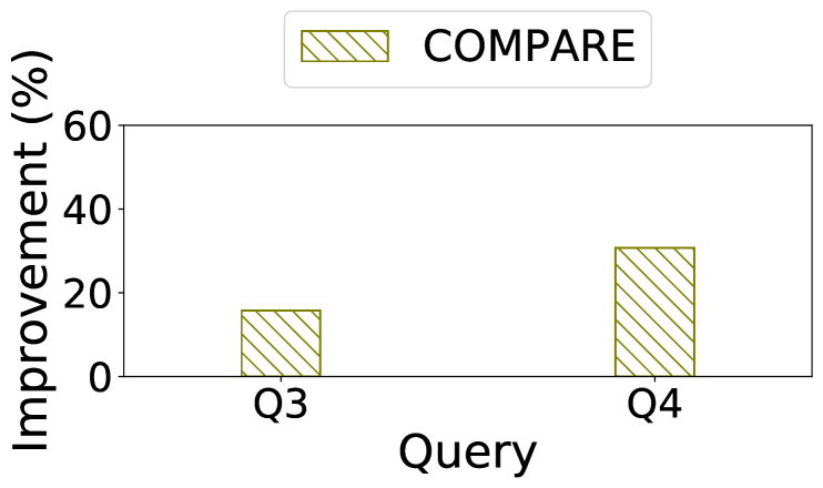
(a) Join pushdown

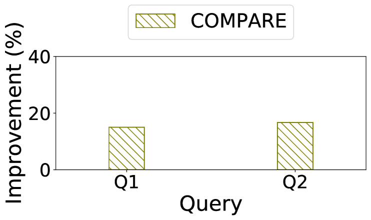
(b) Aggregate pushdown

Figure 13: Pushdown logical optimizations

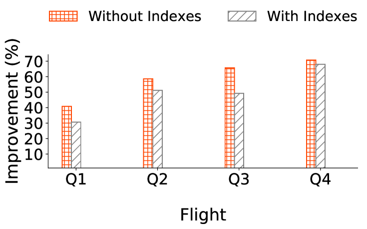
Figure 14: Impact of adding non-clustered indexes on referenced columns and removing other columns

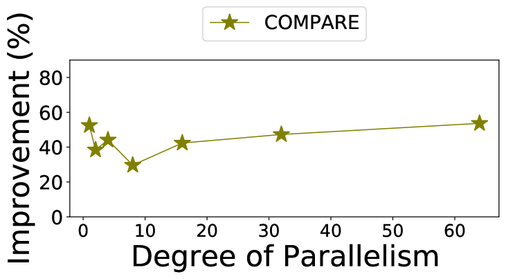
(a) Varying DOP

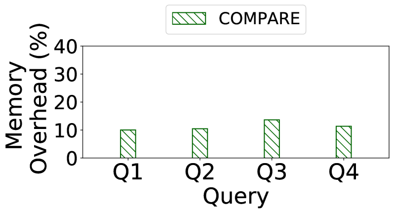
(b) Memory consumption

Figure 15: Impact of Parallelism and Memory Overhead

Figure 15(b) shows the additional overhead in committed memory usage of Compare w.r.t. to SQL Server for each of the queries. Although Compare uses additional data-structures for maintaining segment-aggregates, and bounds in the priority queue, the overhead is minimal ($<$ 13%) compared to the memory already used by the system for sorting and maintaining aggregates which are common to all approaches. Moreover, the execution engine reuses the memory already committed by the downstream operators in the plan, instead of allocating new memory. Thus, the total memory used during query processing is bounded by the maximum memory used by any operator in the plan.

9 Related Work

Visual Analytics. Our work has been motivated by many recent visual analytic tools [19, 47, 43, 49, 31] where comparing subsets or groups of tuples using a deviation-based measures (e.g., $L_{p}$ norms) is the common theme. Unfortunately, as discussed in Section 1 these tools either retrieve the data into a middleware or issue complex SQL queries for comparison, both approaches do not scale to large datasets. As a result, recent work [45, 50, 20] have called for supporting new abstractions and query optimization techniques for addressing the impedance mismatch between relational databases and analytic tasks—our work is a concrete step in this direction.

OLAP. Damianos et al. have proposed grouping variables and operations such as MD-Join [13, 14] for succinctly expressing complex aggregate queries such as finding products with sales above average sales. Similarly, CUBE [22], GROUPING SETs [51], Semantic Group By [44] allow flexible specification and optimization of group by queries. In our work, we extend grouping of tuples to support (i) easier and more direct specification of comparison between groups of tuples using complex aggregate expressions (e.g., $L_{p}$ norms), and (ii) jointly optimize both aggregation and comparison between groups of tuples. Sarawagi et al. have proposed techniques for interactive browsing of interesting cells in data cube [39, 41]. Similarly, These work suggest raw aggregates that are informative given past browsing, or those that show a generalization or explanation of a specific cell. In contrast, we provide extensions to traditional query optimization and execution layers of relational databases to support comparative queries like other SQL queries. Similar to our approach, there have been database extensions [38, 23, 26, 33], the most recent being the DIFF operator [6], that support association and frequent pattern mining. While our focus is on aggregate distance measures such as $L_{p}$ norms (our focus), we share their goal that with an extended syntax, complex analytic queries are easier to write and optimize.

Similarity Join. There has been work on similarity join that use set similarity functions such as edit distance, Jaccard similarity, cosine similarity or their variants to join two relations [40, 21, 37, 11, 15, 9]. While these work are based on measuring set overlap or edit distance between strings, Compare optimizes aggregate distance functions between groups of tuples such as Euclidean distance, requiring fundamentally different execution techniques. Similarly, there is a vast body of work on top-k query processing [25], including ones that extend relational databases  [16, 46, 29, 24]. While these work rank each tuple independently based on an aggregate expression, our focus is on ranking groups of tuples by comparing them with other groups of tuples in the same relation.

Spatial Databases. Finally, spatial databases such as PostGIS [52] extend traditional databases to optimize for storage and querying of spatial data. The similarity search queries supported is spatial databases (e.g.,  [34]) operate in a different settings from ours. First, the physical design is typically optimized to store all information (e.g., sales) for each entity (e.g., product) required for distance computation as a single object, thus no grouping or sorting of tuples is typically required at runtime. In addition, spatial indexes such as R-Tree are built to optimize for search at runtime. In contrast, our work is meant for supporting ad hoc similarity search queries over traditional databases, which are typically used as back-end for BI tools such as Power BI and Tableau.

10 Conclusion

In this work, we introduce Compare, a complex operator that concisely captures comparison between groups of tuples using aggregated distance measures. We introduce physical optimizations within the execution engine and extend the query optimizer with new algebraic rules that improve the performance by significantly reducing the number of subset comparisons and intermediate data size. Together, these logical and physical optimizations help address the impedance mismatch problem between data exploration systems and relational databases for supporting comparative queries. There are several avenues for future work such as supporting primitives for easily expressing comparison metrics such as Jaccard similarity, cosine similarity, as well as using sampling-based techniques to tighten the bounds on scores for further reducing the number of comparisons.

APPENDIX

A. Proof of Theorem 1

Here, we provide the proof for Theorem 1 stated in Section 5.1.

The proof directly derives from the property of convex function. For a convex $f(x)$,

$k_{1}$$f(x_{1})+k_{2}$$f(x_{2})+...+k_{n}$$f(x_{n})$ $\geq$ $f(k_{1}x_{1}+x_{2},x_{2},...,k_{n}x_{n})$

Let each $x_{i}$ be the value a $|m_{1}-m_{2}|$ resulting from comparing a pair of tuples between two trends, and $n$ be the total number of tuple comparisons. On setting, $k_{i}=1/n$ and $f(x)=|x|^{p}$:

$\frac{|m_{1}-m_{2}|^{p}}{n}\geq|\frac{m_{1}}{n}-\frac{m_{2}}{n}|^{p}$

$\Rightarrow$ AVG (DIFF$(m_{1},m_{2},p))\geq$ DIFF(AVG $(m_{1})$, AVG $(m_{2}),p)$ (by def. of DIFF)
$\square$

B. Formal Description of Bounds Computation

Here, we formally describe how we compute the bounds on scores of Compare using segment aggregates (Section 5.1).

Let $p_{1}$ and $p_{2}$ be two trends having same number of tuples $c$ for which we want to to compute the upper and lower bounds on score. Let $max_{1i}$ and $min_{1i}$ be the maximum and minimum values of attribute $m_{1}$ in segment $i$ of trend $p_{1}$, and similarly $max_{2i}$ and $min_{2i}$ be the maximum and minimum values of $m_{2}$ in segment $j$ in $p_{2}$. Let $c_{i}$ be the number of tuples in segment $i$. For succinctness, we use $\Delta(m_{1},m_{2})$ for DIFF($m_{1},m_{2},p$).

We know that the bounds on the $\Delta_{i}(m_{1},m_{2})$ between segment $i$ in $p_{1}$ and $p_{2}$, is given by:

MAX $(\Delta_{i}(m_{1},m_{2}))\leq\Delta_{i}($MAX $(|max_{1i}-min_{2i}|,|min_{1i}-max_{2i}$|))

MIN $(\Delta_{i}(m_{1},m_{2}))\geq\Delta_{i}(($AVG $(m_{1})$,AVG $(m_{2}))$ (From Theorem 1)

From above we get,

$\Delta_{i}$((AVG $(m_{1})$,AVG $(m_{2}))\leq$ AVG $(\Delta_{i}(m_{1},m_{2}))\leq$ MAX $(\Delta_{i}(m_{1},m_{2}))$

Using the non-negativity and Monotonicity property of DIFF, we can replace the value for each tuple comparison with minimum and maximum bounds to get the bounds on SUM.

$c_{i}.$AVG $(\Delta_{i}(m_{1},m_{2}))\leq$ SUM $(\Delta_{i}(m_{1},m_{2}))\leq c_{i}$ MAX $(\Delta_{i}(m_{1},m_{2}))$

The above bounds over a single pair of segments can be extended to segments using the union bound principle. Let $sum_{i}^{u}$, $max_{i}^{u}$, $min_{i}^{u}$ be the upper bounds, and $sum_{i}^{l}$, $max_{i}^{l}$, $min_{i}^{l}$ be the lower bounds on the score of SUM($\Delta(.)$), MAX($\Delta(.)$), and MIN($\Delta(.)$) on scoring segment $i$ in $p_{1}$ and $p_{2}$. Then, the bounds across all segments can be computed as follows:

$\underset{i}{\text{AVG}}(sum_{i}^{l})$ $\leq$ AVG ($\Delta(.)$) $\leq$ $\underset{i}{AVG}(sum_{i}^{u})$

$c.\underset{i}{\text{SUM}}(\frac{sum_{i}}{c_{i}}^{l}$) $\leq$ SUM $\Delta(.)$) $\leq c.\underset{i}{\text{SUM}}(\frac{sum_{i}}{c_{i}}^{u})$

MIN ($\Delta(.)$) $=$ $\underset{i}{\text{MIN}}(min_{i}^{l})$

MAX ($\Delta(.)$) $=$ $\underset{i}{\text{MAX}}(max_{i}^{u})$

References

- [1] Airline dataset (http://stat-computing.org/dataexpo/2009/the-data.html). [Online; accessed 30-Oct-2015].
- [2] Compare technical report. https://bit.ly/3gnUFAU.
- [3] Powerbi (https://powerbi.microsoft.com/en-us/). [Online; accessed 3-June-2019].
- [4] Powerbi (https://www.tableau.com/products/new-features/explain-data). [Online; accessed 3-June-2020].
- [5] Tableau public (www.tableaupublic.com/). [Online; accessed 11-Nov-2019].
- [6] F. Abuzaid, P. Kraft, S. Suri, E. Gan, E. Xu, A. Shenoy, A. Ananthanarayan, J. Sheu, E. Meijer, X. Wu, et al. Diff: a relational interface for large-scale data explanation. Proceedings of the VLDB Endowment, 12(4):419–432, 2018.
- [7] S. Agarwal, R. Agrawal, P. M. Deshpande, A. Gupta, J. F. Naughton, R. Ramakrishnan, and S. Sarawagi. On the computation of multidimensional aggregates. In VLDB, volume 96, pages 506–521, 1996.
- [8] R. Agrawal, C. Faloutsos, and A. Swami. Efficient similarity search in sequence databases. In International conference on foundations of data organization and algorithms, pages 69–84. Springer, 1993.
- [9] A. Arasu, V. Ganti, and R. Kaushik. Efficient exact set-similarity joins. In Proceedings of the 32nd international conference on Very large data bases, pages 918–929. VLDB Endowment, 2006.
- [10] C. Böhm and F. Krebs. The k-nearest neighbour join: Turbo charging the kdd process. Knowledge and Information Systems, 6(6):728–749, 2004.
- [11] C. Bohm and H.-P. Kriegel. A cost model and index architecture for the similarity join. In Proceedings 17th International Conference on Data Engineering, pages 411–420. IEEE, 2001.
- [12] P. Buono, A. Aris, C. Plaisant, A. Khella, and B. Shneiderman. Interactive pattern search in time series. In Visualization and Data Analysis 2005, volume 5669, pages 175–187. International Society for Optics and Photonics, 2005.
- [13] D. Chatziantoniou. Using grouping variables to express complex decision support queries. Data & Knowledge Engineering, 61(1):114–136, 2007.
- [14] D. Chatziantoniou and K. A. Ross. Querying multiple features of groups in relational databases. In VLDB, volume 96, pages 295–306, 1996.
- [15] S. Chaudhuri, V. Ganti, and R. Kaushik. A primitive operator for similarity joins in data cleaning. In 22nd International Conference on Data Engineering (ICDE’06), pages 5–5. IEEE, 2006.
- [16] S. Chaudhuri and L. Gravano. Evaluating top-k selection queries. In VLDB, volume 99, pages 397–410, 1999.
- [17] Z. Chen and V. Narasayya. Efficient computation of multiple group by queries. In Proceedings of the 2005 ACM SIGMOD international conference on Management of data, pages 263–274, 2005.
- [18] C. Cunningham, C. A. Galindo-Legaria, and G. Graefe. Pivot and unpivot: Optimization and execution strategies in an rdbms. In Proceedings of the Thirtieth international conference on Very large data bases-Volume 30, pages 998–1009. VLDB Endowment, 2004.
- [19] R. Ding, S. Han, Y. Xu, H. Zhang, and D. Zhang. Quickinsights: Quick and automatic discovery of insights from multi-dimensional data. In Proceedings of the 2019 International Conference on Management of Data, pages 317–332. ACM, 2019.
- [20] J. V. D’silva, F. De Moor, and B. Kemme. Aida: abstraction for advanced in-database analytics. Proceedings of the VLDB Endowment, 11(11):1400–1413, 2018.
- [21] L. Gravano, P. G. Ipeirotis, H. V. Jagadish, N. Koudas, S. Muthukrishnan, D. Srivastava, et al. Approximate string joins in a database (almost) for free. In VLDB, volume 1, pages 491–500, 2001.
- [22] J. Gray, S. Chaudhuri, A. Bosworth, A. Layman, D. Reichart, M. Venkatrao, F. Pellow, and H. Pirahesh. Data cube: A relational aggregation operator generalizing group-by, cross-tab, and sub-totals. Data mining and knowledge discovery, 1(1):29–53, 1997.
- [23] J. Han et al. Dmql: A data mining query language for relational databases. In Proc. 1996 SiGMOD, volume 96, pages 27–34, 1996.
- [24] I. F. Ilyas, W. G. Aref, and A. K. Elmagarmid. Supporting top-k join queries in relational databases. The VLDB Journal—The International Journal on Very Large Data Bases, 13(3):207–221, 2004.
- [25] I. F. Ilyas, G. Beskales, and M. A. Soliman. A survey of top-k query processing techniques in relational database systems. ACM Computing Surveys (CSUR), 40(4):11, 2008.
- [26] T. Imieliński and A. Virmani. Msql: A query language for database mining. Data Mining and Knowledge Discovery, 3(4):373–408, 1999.
- [27] T. Kluyver, B. Ragan-Kelley, F. Pérez, B. E. Granger, M. Bussonnier, J. Frederic, K. Kelley, J. B. Hamrick, J. Grout, S. Corlay, et al. Jupyter notebooks-a publishing format for reproducible computational workflows. In ELPUB, pages 87–90, 2016.
- [28] D. J.-L. Lee, J. Lee, T. Siddiqui, J. Kim, K. Karahalios, and A. Parameswaran. You can’t always sketch what you want: Understanding sensemaking in visual query systems. IEEE transactions on visualization and computer graphics, 2019.
- [29] C. Li, K. C.-C. Chang, I. F. Ilyas, and S. Song. Ranksql: query algebra and optimization for relational top-k queries. In Proceedings of the 2005 ACM SIGMOD international conference on Management of data, pages 131–142. ACM, 2005.
- [30] R. A. K.-l. Lin and H. S. S. K. Shim. Fast similarity search in the presence of noise, scaling, and translation in time-series databases. In Proceeding of the 21th International Conference on Very Large Data Bases, pages 490–501. Citeseer, 1995.
- [31] S. Macke, Y. Zhang, S. Huang, and A. Parameswaran. Adaptive sampling for rapidly matching histograms. Proceedings of the VLDB Endowment, 11(10):1262–1275, 2018.
- [32] R. O. Nambiar and M. Poess. The making of tpc-ds. In Proceedings of the 32nd international conference on Very large data bases, pages 1049–1058. VLDB Endowment, 2006.
- [33] A. Netz et al. Integrating data mining with sql databases: Ole db for data mining. In ICDE’01, pages 379–387. IEEE, 2001.
- [34] D. Papadias, Y. Tao, K. Mouratidis, and C. K. Hui. Aggregate nearest neighbor queries in spatial databases. ACM Transactions on Database Systems (TODS), 30(2):529–576, 2005.
- [35] D. Rafiei and A. Mendelzon. Similarity-based queries for time series data. In Proceedings of the 1997 ACM SIGMOD international conference on Management of data, pages 13–25, 1997.
- [36] A. Rajaraman and J. Ullman. Finding similar items. Mining of massive datasets, 77:73–80, 2010.
- [37] K. Ramasamy, J. M. Patel, J. F. Naughton, and R. Kaushik. Set containment joins: The good, the bad and the ugly. In VLDB, pages 351–362, 2000.
- [38] S. G. Rao, A. Badia, and D. Van Gucht. Providing better support for a class of decision support queries. In ACM SIGMOD Record, volume 25, pages 217–227. ACM, 1996.
- [39] S. Sarawagi. Explaining differences in multidimensional aggregates. In VLDB, volume 99, pages 7–10, 1999.
- [40] S. Sarawagi and A. Kirpal. Efficient set joins on similarity predicates. In Proceedings of the 2004 ACM SIGMOD international conference on Management of data, pages 743–754. ACM, 2004.
- [41] S. Sarawagi and G. Sathe. i3: intelligent, interactive investigation of olap data cubes. ACM SIGMOD Record, 29(2):589, 2000.
- [42] D. W. Scott. Sturges’ rule. Wiley Interdisciplinary Reviews: Computational Statistics, 1(3):303–306, 2009.
- [43] T. Siddiqui, A. Kim, J. Lee, K. Karahalios, and A. Parameswaran. Effortless data exploration with zenvisage: an expressive and interactive visual analytics system. Proceedings of the VLDB Endowment, 10(4):457–468, 2016.
- [44] M. Tang, R. Y. Tahboub, W. G. Aref, M. J. Atallah, Q. M. Malluhi, M. Ouzzani, and Y. N. Silva. Similarity group-by operators for multi-dimensional relational data. IEEE Transactions on Knowledge and Data Engineering, 28(2):510–523, 2015.
- [45] N. Tang, E. Wu, and G. Li. Towards democratizing relational data visualization. In Proceedings of the 2019 International Conference on Management of Data, pages 2025–2030. ACM, 2019.
- [46] P. Tsaparas, T. Palpanas, Y. Kotidis, N. Koudas, and D. Srivastava. Ranked join indices. In Proceedings 19th International Conference on Data Engineering (Cat. No. 03CH37405), pages 277–288. IEEE, 2003.
- [47] M. Vartak et al. Seedb: Efficient data-driven visualization recommendations to support visual analytics. VLDB, 8(13), Sept. 2015.
- [48] M. Wattenberg. Sketching a graph to query a time-series database. In CHI ’01 Extended Abstracts on Human Factors in Computing Systems, CHI EA ’01, pages 381–382, New York, NY, USA, 2001. ACM.
- [49] K. Wongsuphasawat, Z. Qu, D. Moritz, R. Chang, F. Ouk, A. Anand, J. Mackinlay, B. Howe, and J. Heer. Voyager 2: Augmenting visual analysis with partial view specifications. In Proceedings of the 2017 CHI Conference on Human Factors in Computing Systems, pages 2648–2659. ACM, 2017.
- [50] E. Wu, L. Battle, and S. R. Madden. The case for data visualization management systems: vision paper. Proceedings of the VLDB Endowment, 7(10):903–906, 2014.
- [51] M. Zaharioudakis, R. Cochrane, G. Lapis, H. Pirahesh, and M. Urata. Answering complex sql queries using automatic summary tables. In Proceedings of the 2000 ACM SIGMOD international conference on Management of data, pages 105–116, 2000.
- [52] L. Zhang and J. Yi. Management methods of spatial data based on postgis. In 2010 Second Pacific-Asia Conference on Circuits, Communications and System, volume 1, pages 410–413. IEEE, 2010.