Computation of Reachable Sets Based on Hamilton-Jacobi-Bellman Equation with Running Cost Function
This work has been submitted to the IEEE for possible publication. Copyright may be transferred without notice, after which this version may no longer be accessible.
Abstract
A novel method for computing reachable sets is proposed in this paper. In the proposed method, a Hamilton-Jacobi-Bellman equation with running cost function is numerically solved and the reachable sets of different time horizons are characterized by a family of non-zero level sets of the solution of the Hamilton-Jacobi-Bellman equation. In addition to the classical reachable set, by setting different running cost functions and terminal conditions of the Hamilton-Jacobi-Bellman equation, the proposed method allows to compute more generalized reachable sets, which are referred to as cost-limited reachable sets. In order to overcome the difficulty of solving the Hamilton-Jacobi-Bellman equation caused by the discontinuity of the solution, a method based on recursion and grid interpolation is employed. At the end of this paper, some examples are taken to illustrate the validity and generality of the proposed method.
Keywards: Reachability, Hamilton-Jacobi-Bellman equation, Running cost function, Level set, Numerical method.
1 Introduction
The methods to analyze linear systems have been reasonably mature, some crucial characteristics such as stability, controllability and observability have been systematically and strictly defined. Also, the analyses on these characteristics have become the common steps in solving many engineering problems. However, for nonlinear systems, these characteristics are quite difficult to be defined and analyzed [1], such that for some nonlinear systems, their behaviors are difficult to predict.
Reachability analysis is an effective method to study the behavior of nonlinear control systems. By applying reachability analysis, one can solve a variety of engineering problems, especially those involving system safety [2, 3, 4], feasibility [5], and control law design [6, 7]. In reachability analysis, one specifies a set in the state space as the target set and then aims to find a set of initial states of the trajectories that can reach the target set within a given time horizon [8, 9]. Such a set is referred to as the reachable set. However, finding reachable sets is a challenging task, which involves various aspects such as computation and data storage. The most intuitive approach is to verify each point in the state space one by one, however, this approach often consumes a lot of time due to the diversity of system states and control inputs [10, 11]. Therefore, formal verification methods are needed.
Unfortunately, it is nearly impossible to compute reachable sets using a analytical approach, except for some special problems [12]. In recent years, various numerical methods have been proposed, which can be divided into two categories: the Lagrangian methods [13, 14, 15, 16] and the methods based on state space discretization [17, 18, 19, 10, 2, 3]. The former can solve the reachability problems of high-dimensional systems, but has high requirements on the form of the control system, and thus is mainly used to solve linear problems. The latter has less requirements on the form of the control system and can therefore be used for nonlinear systems. It is this universality that makes the methods based on state space discretization more widely used in engineering, and the level set method [8, 10, 2, 3] is a representative of them.
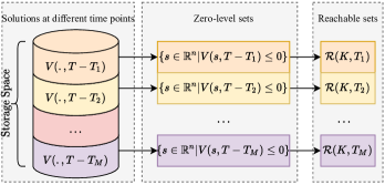
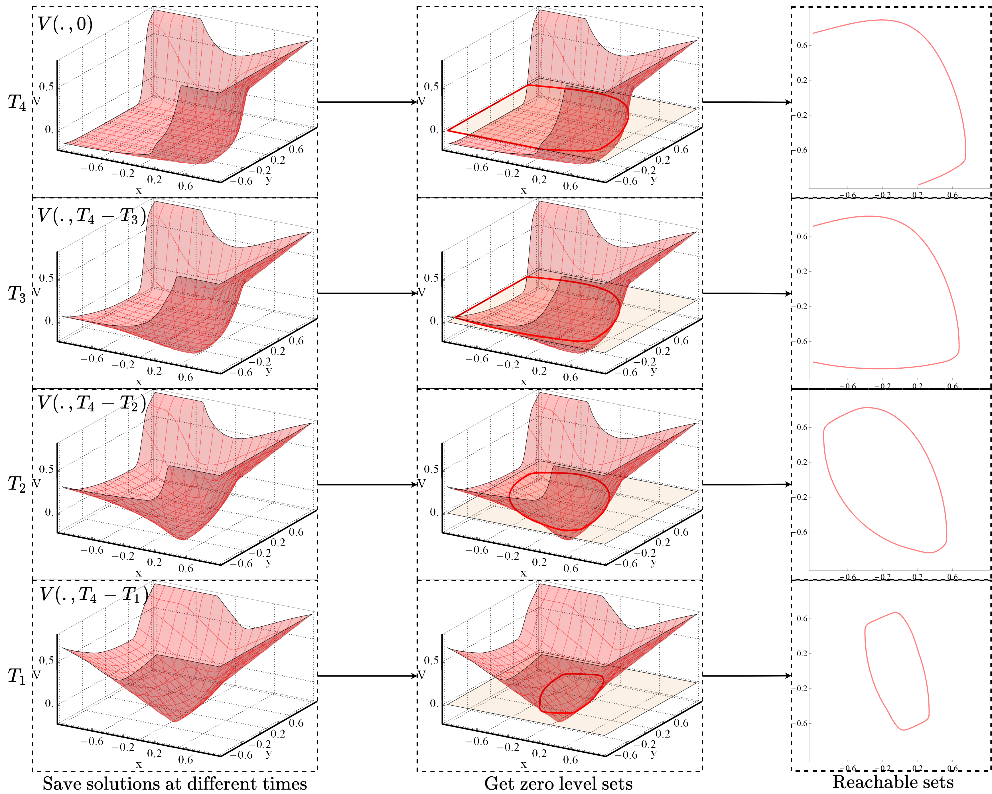
In the level set method, a Hamilton-Jacobi-Bellman (HJB) equation without running cost function is constructed, and the terminal condition of this equation is set to the signed distance function of the target set. Then the state space is discretized into a Cartesian grid structure and the HJB equation is numerically solved. During the computation, the values of the equation’s solutions at the grid points are stored in an array that has the same dimensions as the state space. Finally, the reachable set is characterized as the zero-level set of the solution.
The principle of the level set method determines that its storage space requirements are quite demanding. To save the reachable set of a given time horizon, one needs to save the solution of the HJB equation at a certain time point, the memory required grow significantly with an increase in the problem’s dimension [6, 20, 21]. To save the reachable sets under different time horizons, one needs to save the solutions of the HJB equation at different time points, which in turn leads to a multiple increase in storage space consumption. In addition, in the level set approach, saving the solutions of the HJB equation at multiple moments is also necessary for designing the control law [6, 8, 22]. These limitations restrict the development and application of the level set method to some extent.
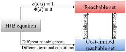
In order to overcome the above-mentioned limitations, this paper proposes a new method to compute reachable sets. In the proposed method, a HJB equation with running cost function is numerically solved, and the reachable sets under different time horizons can be characterized by different non-zero level sets of the solution of the HJB equation at a certain time point. Such a mechanism can significantly reduce the consumption of storage space and facilitate the design of control law. In addition, more generalized reachability problems can be solved by setting different running cost functions and terminal conditions. In these problems, a performance index can be constructed, which is a combination of a Lagrangian (the time integral of a running cost) and an endpoint cost. The aim is to find a set of initial states of the trajectories that can reach the target set before the performance index increasing to the given admissible cost. In this paper, such a set is referred to as a cost-limited reachable set.
In summary, the main contributions of this paper are as follows:
-
(1)
A novel method for computing reachable sets based on the HJB equation with a running cost function is proposed. This method can significantly reduce the storage space consumption and bring convenience to the control law design.
-
(2)
The reachability problem is generalized by setting different running cost functions and terminal conditions, and the definition of cost-limited reachable set is put forward.
-
(3)
To overcome the discontinuity of the solution of the HJB equation, a numerical method based on recursion and grid interpolation is applied to solve the HJB equation.
The structure of this paper is as follows. Section II briefly introduces the reachability problem and the level set method. Section III describes the method to construct the HJB equation of the proposed method and the representation of the reachable set. Section IV generalizes the reachability problem and presents the definition of cost-limited reachable set, and also introduces the method to design control law. A method to solve the HJB equation is proposed in Section V and some numerical examples are given in Section VI. The results are summarized in Section VII.
2 Preliminaries
2.1 Reachability problem
Consider a continuous time control system with fully observable state:
| (1) |
where is the system state, is referred to as the control input. The function is bounded. Let denote the set of lebesgue measurable functions from the time interval to . Then, given the initial state at time , , the evolution of system (1) in time interval can be denoted as a continuous trajectory and . Given a target set and a time horizon , The definition of reachable set is [14, 8]:
Definition 1 (Reachable set).
| (2) | ||||
2.2 Level set method
In level set method, the following HJB equation about is numerically solved:
| (5) |
where is bounded and Lipschitz continuous, and satisfies . The solution is approximated on a Cartesian grid of the state space. The reachable set is represented as the zero level set of function , i.e.
| (6) |
Based on this principle, several mature toolboxes have been developed [23, 24, 3] and applied to many practical engineering problems, such as flight control systems [25, 26, 27, 7, 28], ground traffic management systems [29, 30, 31], air traffic management systems [2, 3, 32], etc.
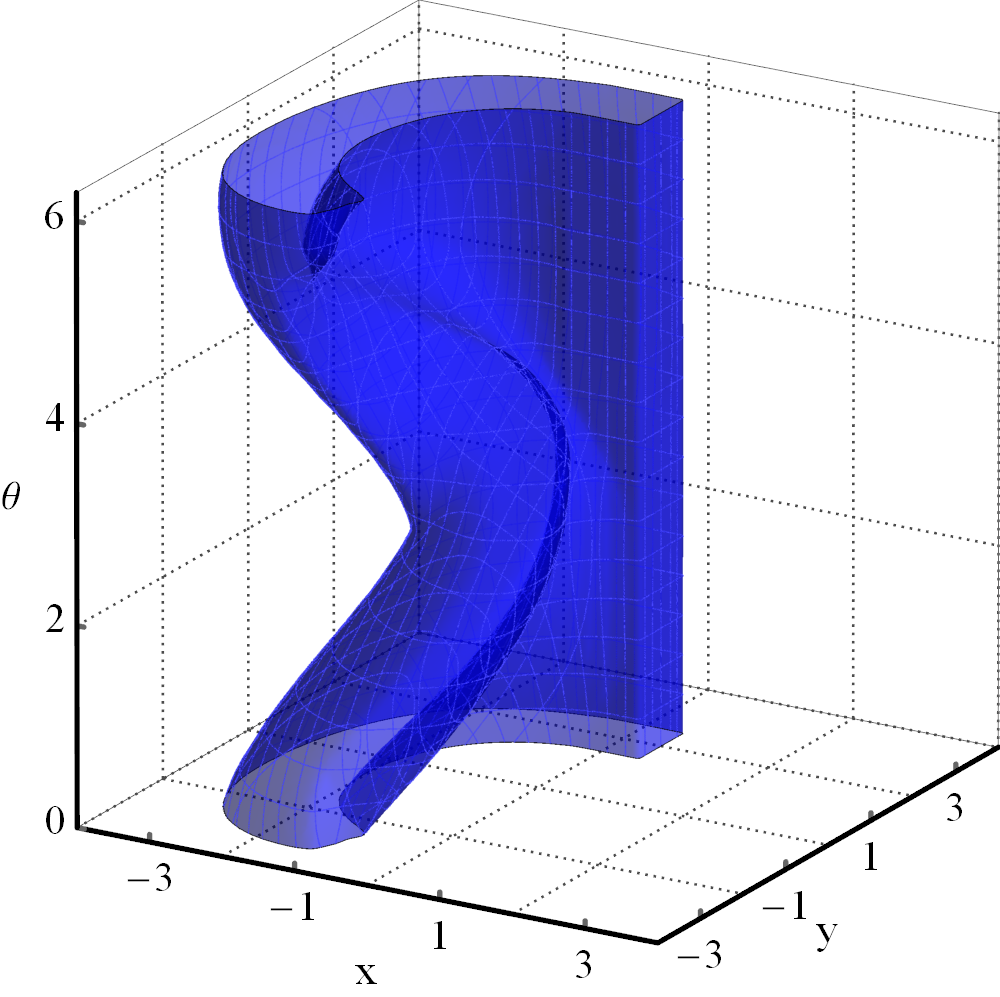
Denote the number of grid points in the th dimension of the Cartesian grid as , then the storage space consumed to save is proportional to . It should be noted that, for , the expressions of the reachable sets of these time horizons are as follows:
| (7) | ||||
Since the value functions are each different, the storage space consumption required to save these reachable sets is proportional to , see Fig. 1.
3 Method Based on HJB Equation with Running Cost Function
3.1 Reachability problem and optimal control
Consider a case where the control input aims to transfer the system state to the target set in the shortest possible time. In this case, if a trajectory can reach the target set in the time horizon , then the initial state of this trajectory belongs to the reachable set. Therefore, a value function can be constructed as follows:
| (8) |
where is a running cost function and . then the reachable set can be characterized by the -level set of , i.e.
| (9) |
Define a modified dynamic system:
| (10) |
and a modified running cost function:
| (11) |
Given the state at time , , the evolution of system (10) in time interval can be denoted as and .
Theorem 1.
For any , holds.
Proof.
The maximum of the value function is:
| (17) |
The trajectories of system (10) correspond to the same trajectories as the evolution of system (1) as long as it evolves outside the target set, once a trajectory of system (10) touches the border of the target set, it stays at the border of the target set and the modifies running cost function is set to . Consequently,
| (18) |
Therefore,
| (19) | ||||
Theorem 1 states that in the region , and are equal, and for any , the reachable set can also be expressed as:
| (20) |
In addition, for , the reachable sets can be represented as different level sets of the value function , and simply save to save all these reachable sets, i.e.
| (21) | ||||
3.2 Construction of HJB equation
Based on system (10) and running cost function (11), an HJB equation with running cost function can be constructed:
| (22) |
Theorem 2.
The solution of Eq. (22) at time and are equivalent, i.e., for any ,
| (23) |
Proof.
When , the following equation holds:
| (24) |
From the definition of , this function is a cost-to-go function on the time interval . According to Bellman’s principle of optimality [33], for any a small enough , the cost-to-go function should satisfy the following equation:
| (25) | ||||
Since
| (26) | ||||
Substituting Eq. (26) into Eq. (25) yields the following equation:
| (27) |
Combining Eq. (24) and Eq. (27), the form is exactly the same as that of Eq. (22).
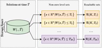
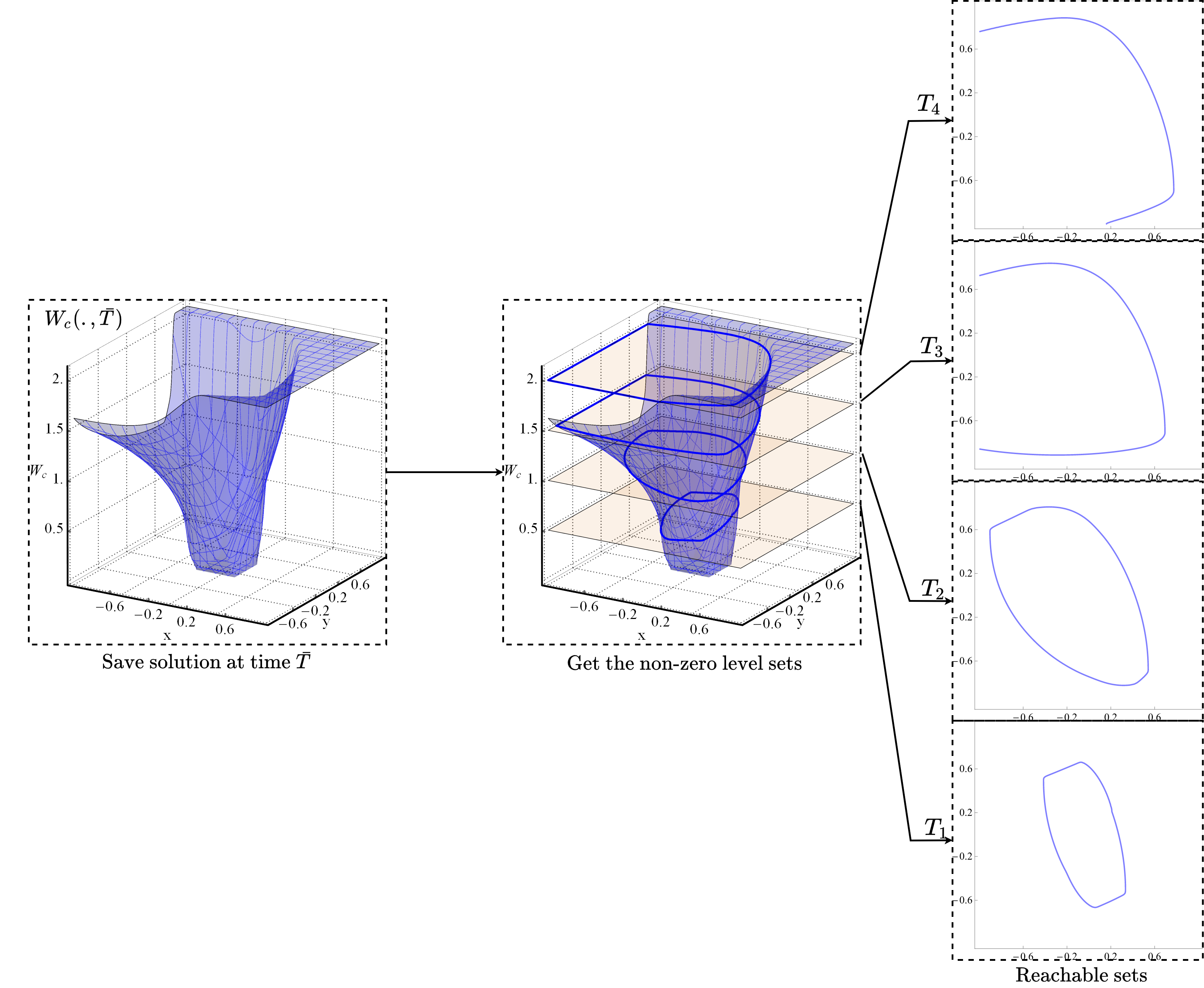
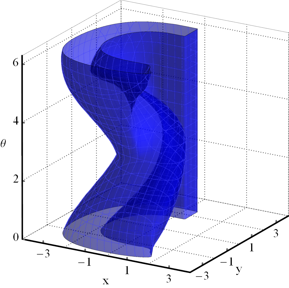
Theorem 2 indicates that the reachable sets of different time horizons can be represented by different level sets of the solution of Eq. (22), i.e.
| (28) | ||||
Fig. 2 illustrates the way to save the reachable sets by the proposed method.
4 Generalization of reachability problems
In the previous section, the running cost function and the terminal condition of HJB equation are quite special. In fact, the HJB equation can also be used for more general reachability problems by setting different running cost functions and terminal conditions. This section introduces a novel type of reachability problems.
4.1 Definition of cost-limited reachable set
A general running cost function is a scalar function of state and control input, denoted as
| (29) |
In this section, we assume that:
Assumption 1.
holds, where is a positive real number.
The above-mentioned assumption is easily satisfied in engineering practice, such as the fuel consumption and path length per unit time are positive.
The performance index of the evolution of system (1) initialized from at time under control input in time interval is denoted as:
| (30) | ||||
where is the endpoint cost function. Given a target set and an admissible cost , the cost-limited reachable set can be defined:
Definition 2 (Cost-limited reachable set).
| (31) | ||||
where ”” is the logical operator ”AND”.
Informally, under Assumption 1, the performance index increases with the increasing of time, the cost-limited reachable set is a set of initial states of trajectories that can be reach the target set before the performance index increasing to the given admissible cost.
Remark 1.
4.2 Computation of cost-limited reachable set
Consider a case where the controller aims to transfer the system state to the target set with the least possible cost. If a trajectory can enter the target set before the performance index increasing to the given admissible cost, its initial state must in the cost-limited reachable set. Similar to Eq. (8), a value function can be constructed as follows:
| (32) |
The cost-limited reachable set can be represented as the -level set of function , i.e.
| (33) |
Construct a modified running cost function on the basis of Eq. (29):
| (34) |
Similar to Eq. (16), based on the modified running cost function (34) and the modified system (10), the following value function can be constructed:
| (39) |
Theorem 3.
For any , holds.
Proof.
Theorem 4.
the value function can be obtained by solving the following HJB equation about :
| (43) |
It follows from Theorem 3 and Theorem 4 that, for , the cost-limited reachable sets can be represented as different level sets of and all these sets can be saved by saving , i.e.
| (44) | ||||
See Fig. 4.

4.3 Control law design
4.3.1 Control law in the level set method
In the level set method, at time , the optimal control input at state is [8, 6]:
| (45) |
For any , the trajectory initialized from can reach the target set under control law (45) in time . Since varies with time , it is required to save at each time point in time interval to implement this control law. This also requires a large amount of storage space.
4.3.2 Control law in the proposed method
The following control law ensures that the trajectory of the system enters the target set at the smallest performance index:
| (46) |
5 Method to Solve HJB Equation
Since Eq. (22) is a special form of Eq. (43), this section introduces the method of solving Eq. (43). The analytical solution of Eq. (43) is usually difficult to obtain. To make matters worse, the solution of Eq. (43) is not everywhere differentiable and sometimes even discontinuous, which leads to the difficulty in obtaining the viscosity solution as well [34]. In the current research, a numerical method based on recursion and interpolation is introduced.
5.1 Recursive formula of the solution
Divide the time interval into subintervals of length . If is small enough, can be regarded as a constant in interval for , and system (1) can be converted into the following discretized form:
| (48) |
Thus, the discrete form of system (10) is:
| (49) | ||||
The definite integral of the running cost function (29) over the time interval is denoted as:
| (50) | ||||
and the integral of the modified running cost function (34) is denoted as:
| (51) | ||||
The recursive formula of the solution of Eq. (43) is:
| (52) | ||||
5.2 Approximation of the solution
This subsection introduces a method based on interpolation to approximate . The proposed method is similar to the level set method in this respect. First, a rectangular computational domain, denoted as , needs to be specified in the state space and divided into a Cartesian grid structure. The value of the solution at the grid point is stored in an array with the same dimensions as the state space, and is approximated by the grid interpolation. Take a two-dimensional system as an example, and denote the system state as . The pseudocode of the proposed method is shown in Algorithm 1.
6 Numerical Examples
This section provides two examples, the first one about the reachable set of a two-dimensional system, to visually demonstrate the superiority of the proposed method in terms of storage space consumption. The second example is about the cost-limited reachable sets in a practical engineering problem to demonstrate the generality of the proposed method.
6.1 Two-dimensional system example
Consider the following system:
| (57) |
where is the system state, is the control input. The target set . The given time horizons are . The task is to compute the reachable set corresponding to each time horizon. Table 1 outlines the parameters that are specified for the reachable set computation.
| Parameter | Setting |
|---|---|
| Computational domain | |
| Number of grid points | |
| Number of time steps | |
| Time step size |
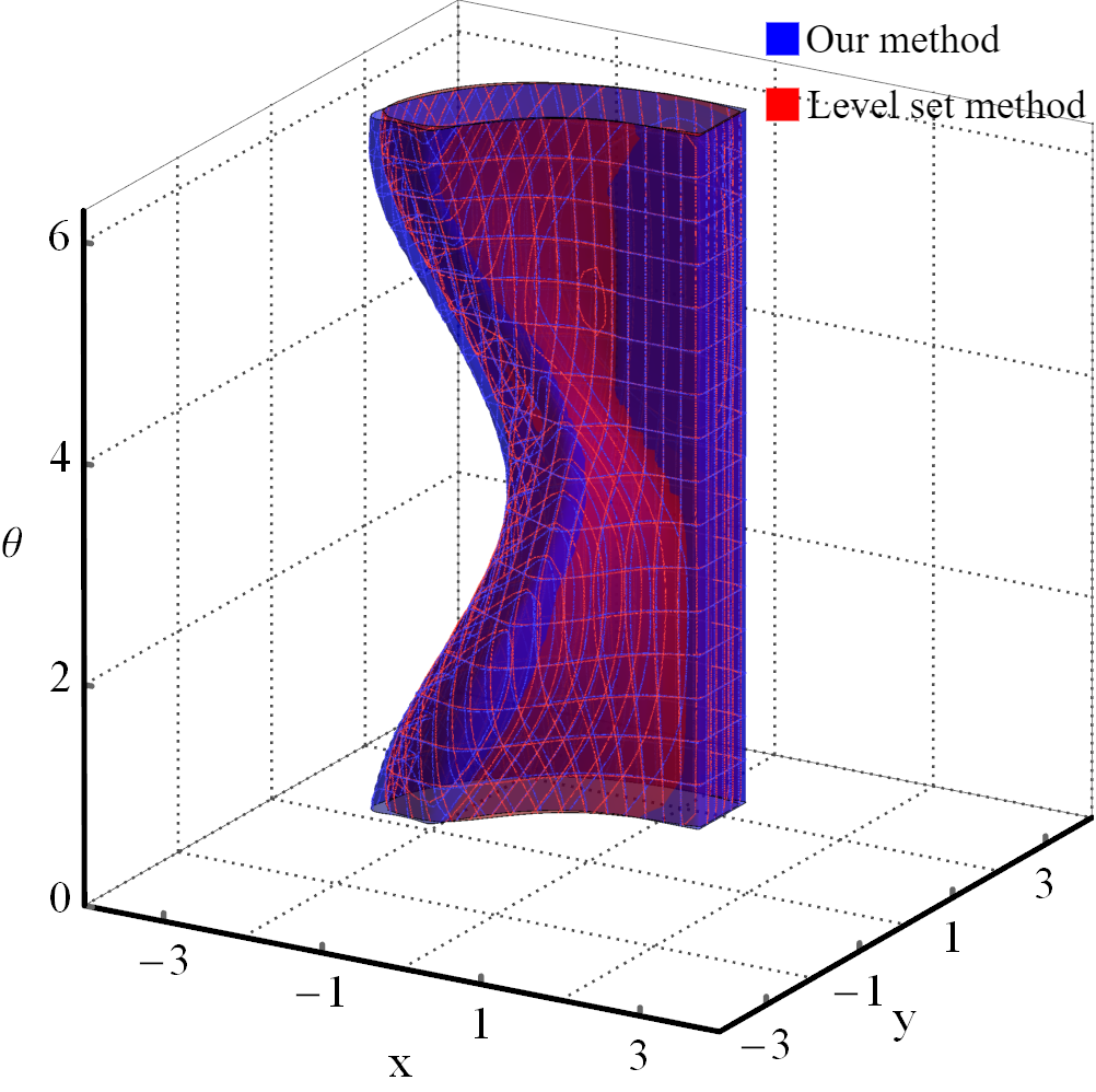
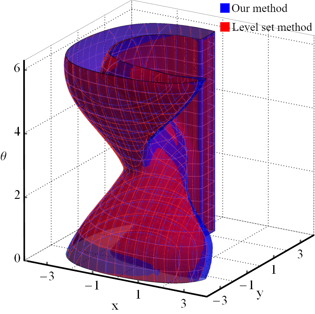
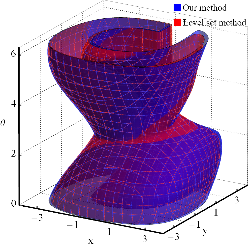
As this example computes the reachable sets, the running cost function is set to and the endpoint cost function is set to . Fig. 5 shows the computation results of the proposed method and compares them with those of the level set method (The computational domain and the number of grids used in the level set method are the same as in our method, and the terminal condition of the HJB equation in the level set method is set as ).
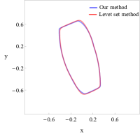
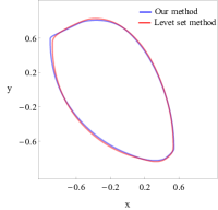
As can be seen in Fig. 5, the results of the proposed method and those of the level set method almost coincide, which indicates that the proposed method has a high accuracy.
Fig. 6 visualizes the storage forms of reachable sets in the proposed method as well as in the level set method. Our method only needs to save function , while the level set method needs to save , , , and , consuming four times more storage space than our method.
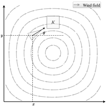
6.2 Planar flight example
A flight vehicle moves in a plane wind field, the vehicle is modeled as a simple mass point with fixed linear velocity and controllable heading angular velocity. The behavior of the vehicle in still air is described by the following equation:
| (58) | ||||
where and are the position and heading angle of the vehicle respectively, and is the control input. The wind speed at position is determined by the following vector field:
| (63) |
Then, the behavior of the vehicle in the wind field is:
| (70) |
where . The target set and task area depend only on and and include any positions in the following rectangular regions in plane:
| (71) | |||
| (72) |
See Fig. 7 for a visual depiction of the problem.
The running cost is a weighted sum of the time consumption and the length of flight path per unit time, i.e.:
| (73) |
where is the weight of the length of flight path. The admissible costs are . We consider two cases:
-
(1)
and .
-
(2)
and
6.2.1 Case (1)
In the first case, the running cost function is constant equal to 1 and the endpoint cost is constant equal to 0, the cost-limited reachable sets degenerate into reachable set. The solver setups of this case are summarized in Table 2.
| Parameter | Setting |
|---|---|
| Computational domain | |
| Number of grid points | |
| Number of time steps | |
| Time step size |
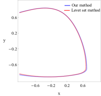
Fig. 8 shows the computational results of our method and the comparison with the level set method. As can be seen, in this example, the results of the proposed method and the level set method are also in excellent agreement.
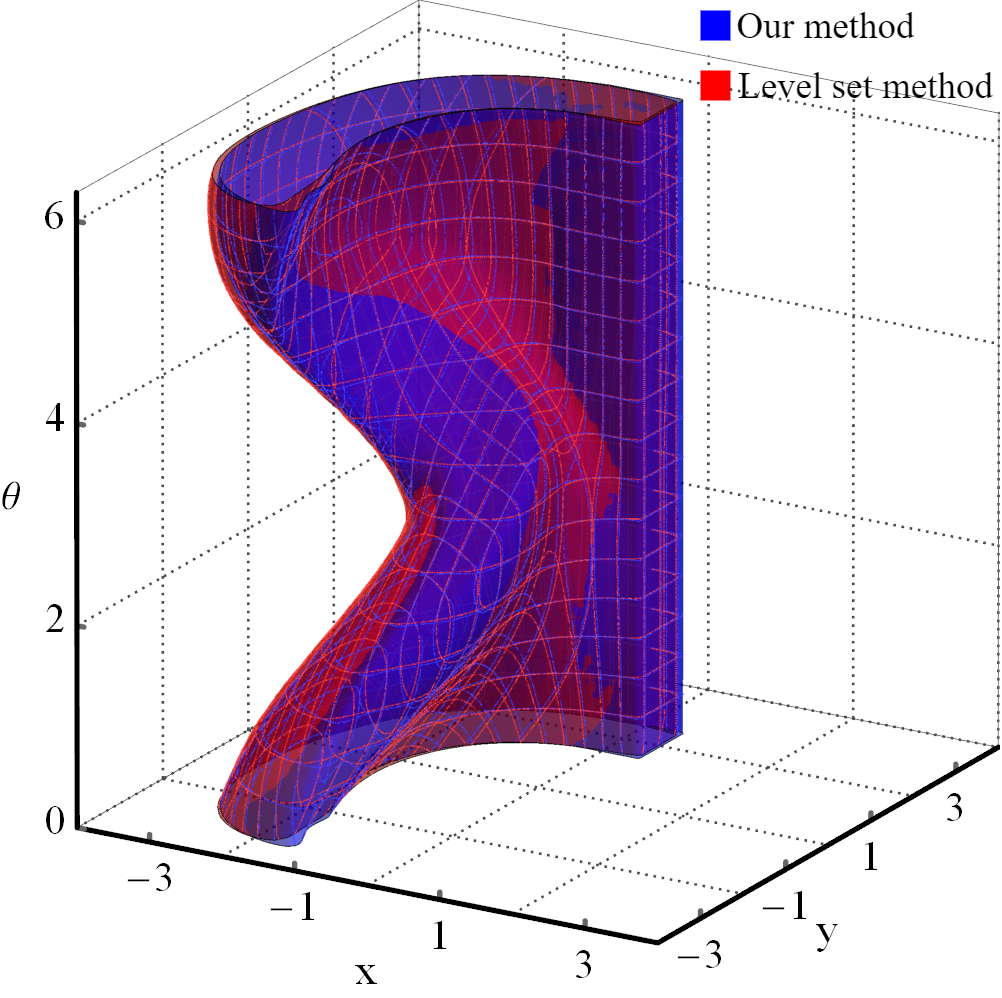
6.2.2 Case (2)
In this case, the cost-limited reachable sets no longer degenerate to reachable sets and therefore cannot be computed using the level set method, but can still be computed using the proposed method.
In this case, , . According to line 3 of Algorithm 1, should satisfy the following inequalities:
| (74) |
Therefore, is set to 4.1. The solver setups of this case are listed in Table 3.
| Parameter | Setting |
|---|---|
| Computational domain | |
| Number of grid points | |
| Number of time steps | |
| Time step size |
The computation results are shown in Fig. 9.
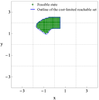
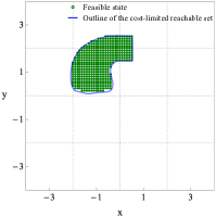
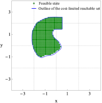
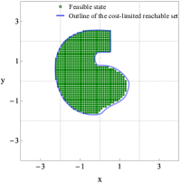
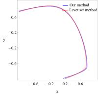
In order to verify the correctness of the results and the validity of the control law in Eq. (47), we test some states in slice of the state space to determine whether the trajectories initialized from these states can reach the target set before the performance index increasing to the given admissible costs under this control law. The verification results are shown in Fig. 10. It can be seen that the outlines of the cost-limited reachable sets and the borders of the areas marked by the green circles almost coincide, which shows the accuracy of the computation of the cost-limited reachable sets and the validity of the control law in Eq. (47).
7 Conclusions
This paper proposes a new method for computing reachable sets. In the proposed method, the reachable sets of different time horizons are represented by different non-zero level sets of a HJB equation with a running cost function. This approach significantly reduces the storage space consumption for saving reachable sets and designing control laws.
In addition to being able to solve the classical reachability problems, the proposed method can also solve more generalized reachability problems by setting different operating cost functions and different terminal conditions for the HJB equation. The reachable sets in such problems are referred to in this paper as cost-limited reachable sets
In order to overcome the discontinuity of the solution of the HJB equation, the current research adopts a method based on recursion and grid interpolation for solving the HJB equation. The paper concludes with some examples to illustrate the effectiveness and generality of the proposed method.
However, the proposed method has some potential for improvement. The main drawback of the proposed method, and also the main drawback of the level set method, lies in the exponential growth of memory and computational cost as the system dimension increases. Some approaches have been proposed to mitigate these costs, such as splitting the original high-dimensional system into multiple low-dimensional subsystems based on the dependencies between the system states [11, 21] or the time-scale principle [28, 35]. These approaches will be considered in our future works.
Acknowledgements
The authors would like to thank the anonymous reviewers, associate editor, and editor for their valuable and constructive comments and suggestions.
References
- [1] H. Khalil, Nonlinear Systems (3rd Ed.). Upper Saddle River: Prentice-Hall Inc., 01 2001.
- [2] M. Chen, S. Bansal, J. F. Fisac, and C. J. Tomlin, “Robust sequential trajectory planning under disturbances and adversarial intruder,” IEEE Transactions on Control Systems Technology, vol. 27, DOI 10.1109/TCST.2018.2828380, no. 4, pp. 1566–1582, 2019.
- [3] S. Bansal, M. Chen, K. Tanabe, and C. J. Tomlin, “Provably safe and scalable multivehicle trajectory planning,” IEEE Transactions on Control Systems Technology, DOI 10.1109/TCST.2020.3042815, pp. 1–17, 2020.
- [4] J. F. Fisac, M. Chen, C. J. Tomlin, and S. S. Sastry, “Reach-avoid problems with time-varying dynamics, targets and constraints,” ser. HSCC ’15, DOI 10.1145/2728606.2728612, pp. 11–20. New York, NY, USA: Association for Computing Machinery, 2015.
- [5] A. Chakrabarty, C. Danielson, S. Di Cairano, and A. Raghunathan, “Active learning for estimating reachable sets for systems with unknown dynamics,” IEEE Transactions on Cybernetics, DOI 10.1109/TCYB.2020.3000966, pp. 1–12, 2020.
- [6] H. N. Nabi, T. Lombaerts, Y. Zhang, E. van Kampen, Q. P. Chu, and C. C. de Visser, “Effects of structural failure on the safe flight envelope of aircraft,” Journal of Guidance, Control, and Dynamics, vol. 41, DOI 10.2514/1.G003184, no. 6, pp. 1257–1275, 2018.
- [7] Y. Zhang, C. C. de Visser, and Q. P. Chu, “Database building and interpolation for an online safe flight envelope prediction system,” Journal of Guidance, Control, and Dynamics, vol. 42, DOI 10.2514/1.G003834, no. 5, pp. 1166–1174, 2019.
- [8] J. Lygeros, “On reachability and minimum cost optimal control,” Automatica, vol. 40, DOI 10.1016/j.automatica.2004.01.012, no. 6, pp. 917 – 927, 2004.
- [9] I. M. Mitchell, A. M. Bayen, and C. J. Tomlin, “A time-dependent hamilton-jacobi formulation of reachable sets for continuous dynamic games,” IEEE Transactions on Automatic Control, vol. 50, DOI 10.1109/TAC.2005.851439, no. 7, pp. 947–957, 2005.
- [10] S. Bansal, M. Chen, S. Herbert, and C. J. Tomlin, “Hamilton-jacobi reachability: A brief overview and recent advances,” in 2017 IEEE 56th Annual Conference on Decision and Control (CDC), DOI 10.1109/CDC.2017.8263977, pp. 2242–2253, 2017.
- [11] M. Chen, S. L. Herbert, M. S. Vashishtha, S. Bansal, and C. J. Tomlin, “Decomposition of reachable sets and tubes for a class of nonlinear systems,” IEEE Transactions on Automatic Control, vol. 63, DOI 10.1109/TAC.2018.2797194, no. 11, pp. 3675–3688, 2018.
- [12] T. Gan, M. Chen, Y. Li, B. Xia, and N. Zhan, “Reachability analysis for solvable dynamical systems,” IEEE Transactions on Automatic Control, vol. 63, DOI 10.1109/TAC.2017.2763785, no. 7, pp. 2003–2018, 2018.
- [13] A. B. Kurzhanski and P. Varaiya, “Ellipsoidal techniques for reachability analysis,” in Hybrid Systems: Computation and Control, N. Lynch and B. H. Krogh, Eds., pp. 202–214. Berlin, Heidelberg: Springer Berlin Heidelberg, 2000.
- [14] Y. Chen, J. Lam, Y. Cui, J. Shen, and K.-W. Kwok, “Reachable set estimation and synthesis for periodic positive systems,” IEEE Transactions on Cybernetics, vol. 51, DOI 10.1109/TCYB.2019.2908676, no. 2, pp. 501–511, 2021.
- [15] A. Chutinan and B. Krogh, “Computational techniques for hybrid system verification,” IEEE Transactions on Automatic Control, vol. 48, DOI 10.1109/TAC.2002.806655, no. 1, pp. 64–75, 2003.
- [16] T. Wang, X. Wang, and W. Xiang, “Reachable set estimation and decentralized control synthesis for a class of large-scale switched systems,” ISA Transactions, vol. 103, DOI https://doi.org/10.1016/j.isatra.2020.03.020, pp. 75–85, 2020. [Online]. Available: https://www.sciencedirect.com/science/article/pii/S0019057820301282
- [17] Y. E. Arslantas, T. Oehlschlagel, and M. Sagliano, “Safe landing area determination for a moon lander by reachability analysis,” Acta Astronautica, vol. 128, DOI 10.1016/j.actaastro.2016.08.013, pp. 607–615, 2016.
- [18] R. Helsen, E.-J. van Kampen, C. C. de Visser, and Q. Chu, “Distance-fields-over-grids method for aircraft envelope determination,” Journal of Guidance, Control, and Dynamics, vol. 39, DOI 10.2514/1.G000824, no. 7, pp. 1470–1480, 2016.
- [19] R. Baier, M. Gerdts, and I. Xausa, “Approximation of reachable sets using optimal control algorithms,” Numerical Algebra, Control and Optimization, vol. 3, DOI 10.3934/naco.2013.3.519, 09 2013.
- [20] A. M. Bayen, I. M. Mitchell, M. M. K. Oishi, and C. J. Tomlin, “Aircraft autolander safety analysis through optimal control-based reach set computation,” Journal of Guidance, Control, and Dynamics, vol. 30, DOI 10.2514/1.21562, no. 1, pp. 68–77, 2007.
- [21] I. M. Mitchell, “Scalable calculation of reach sets and tubes for nonlinear systems with terminal integrators: A mixed implicit explicit formulation,” in Proceedings of the 14th International Conference on Hybrid Systems: Computation and Control, DOI 10.1145/1967701.1967718, pp. 103–112. Association for Computing Machinery, 2011.
- [22] J. Ding, J. Sprinkle, C. J. Tomlin, S. S. Sastry, and J. L. Paunicka, “Reachability calculations for vehicle safety during manned/unmanned vehicle interaction,” Journal of Guidance, Control, and Dynamics, vol. 35, DOI 10.2514/1.53706, no. 1, pp. 138–152, 2012.
- [23] I. Mitchell, “A toolbox of level set methods,” Dept. Comput. Sci., Univ. British Columbia, Vancouver, BC, Canada, Tech. Rep., 2004. [Online]. Available: http://www.cs.ubc.ca/~mitchell/ToolboxLS/toolboxLS.pdf
- [24] I. M. Mitchell, “The flexible, extensible and efficient toolbox of level set methods,” Journal of Scientific Computing, vol. 35, DOI 10.1007/s10915-007-9174-4, no. 2, pp. 300–329, 2008.
- [25] Y. Liu, J. Wang, Q. Quan, G.-X. Du, and L. Yang, “Reachability analysis on optimal trim state for aerial docking,” Aerospace Science and Technology, vol. 110, DOI 10.1016/j.ast.2020.106471, p. 106471, 2021.
- [26] C. Livadas and N. A. Lynch, “Formal verification of safety-critical hybrid systems,” in Hybrid Systems: Computation and Control, T. A. Henzinger and S. Sastry, Eds., pp. 253–272. Berlin, Heidelberg: Springer Berlin Heidelberg, 1998.
- [27] S. Vaskov, H. Larson, S. Kousik, M. Johnson-Roberson, and R. Vasudevan, “Not-at-fault driving in traffic: A reachability-based approach,” in 2019 IEEE Intelligent Transportation Systems Conference (ITSC), DOI 10.1109/ITSC.2019.8917052, pp. 2785–2790, 2019.
- [28] A. K. Akametalu, C. J. Tomlin, and M. Chen, “Reachability-based forced landing system,” Journal of Guidance, Control, and Dynamics, vol. 41, DOI 10.2514/1.G003490, no. 12, pp. 2529–2542, 2018.
- [29] C. Livadas, J. Lygeros, and N. Lynch, “High-level modeling and analysis of the traffic alert and collision avoidance system (tcas),” Proc. IEEE, vol. 88, DOI 10.1109/5.871302, pp. 926 – 948, 08 2000.
- [30] C. Tomlin, J. Lygeros, and S. Sastry, “A game theoretic approach to controller design for hybrid systems,” Proc. IEEE, vol. 88, DOI 10.1109/5.871303, pp. 949 – 970, 08 2000.
- [31] S. Bansal, A. Bajcsy, E. Ratner, A. D. Dragan, and C. J. Tomlin, “A hamilton-jacobi reachability-based framework for predicting and analyzing human motion for safe planning,” in 2020 IEEE International Conference on Robotics and Automation (ICRA), DOI 10.1109/ICRA40945.2020.9197257, pp. 7149–7155, 2020.
- [32] Z. Zhong, Y. Zhu, and C. K. Ahn, “Reachable set estimation for takagi-sugeno fuzzy systems against unknown output delays with application to tracking control of auvs,” ISA Transactions, vol. 78, DOI https://doi.org/10.1016/j.isatra.2018.03.001, pp. 31–38, 2018, advanced Methods in Control and Signal Processing for Complex Marine Systems. [Online]. Available: https://www.sciencedirect.com/science/article/pii/S0019057818300958
- [33] S. Dreyfus, “Richard bellman on the birth of dynamic programming,” Operations Research, vol. 50, DOI 10.1287/opre.50.1.48.17791, no. 1, pp. 48–51, 2002.
- [34] M. G. Crandall, “Viscosity solutions of hamilton-jacobi equations,” in Nonlinear Problems: Present and Future, ser. North-Holland Mathematics Studies, A. Bishop, D. Campbell, and B. Nicolaenko, Eds., vol. 61, DOI 10.1016/S0304-0208(08)71044-2, pp. 117–125. North-Holland, 1982.
- [35] I. Kitsios and J. Lygeros, “Aerodynamic envelope computation for safe landing of the hl-20 personnel launch vehicle using hybrid control,” in Proceedings of the 2005 IEEE International Symposium on, Mediterrean Conference on Control and Automation Intelligent Control, 2005., DOI 10.1109/.2005.1467020, pp. 231–236, 2005.